Relativistic and magnetic effects in photo ionization of hydrogen-like ions

Abstract

We investigate the role of relativistic and magnetic corrections in photo ionization of hydrogen-like ions. For hydrogen, the wavelengths of the laser resides in the weakly ultra violet region. For higher nuclear charges, the laser parameters are scaled in a manner which renders the time-dependent Schrödinger equation in the dipole approximation independent of nuclear charge. By comparing with numerical solutions of both the relativistic time-dependent Dirac equation and the non-relativistic Schrödinger equation – with and without magnetic interactions, the influence of these interactions are revealed. Moreover, we investigate to what extent relativistic effects are induced by the relativistic shift in the structure of the ions or by the strong external field. In agreement with a recent work, Ivanova et al., Phys. Rev. A 98, 063402 (2018), we find that the dominant relativistic correction is the former, i.e., the relativistic shift in the binding energy of the ions. However, dynamical relativistic corrections induced by the laser field are also seen – in addition to a significant influence of the magnetic field for the longer wavelengths.

I Introduction

Motivated by experimental breakthroughs, we have seen an increased interest in the theoretical and computational study of relativistic dynamics for atoms and ions exposed to strong laser pulses Di Piazza et al. (2012). Such investigations tend to be quite demanding from a computational point of view as the ionization process is governed by the time-dependent Dirac equation, which typically is quite hard to solve. For this reason, many studies resort to models and approximations – such as the so-called strong field approximation and models of reduced dimensionality. However, also on the theoretical and computational side we have recently seen significant breakthroughs when it comes to fully relativistic descriptions, see, e.g., Braun et al. (1999); Fillion-Gourdeau et al. (2012); Ivanov (2015); Fillion-Gourdeau et al. (2016); Kjellsson et al. (2017a, b); Ivanova et al. (2018); Kjellsson Lindblom et al. (2018). Moreover, it has also been shown how exponential speedup in solving the Dirac equation may be achieved on a quantum computer Fillion-Gourdeau et al. (2017).

The numerical solution of the time-dependent Dirac equation is subject to several issues which its non-relativistic counterpart, the Schrödinger equation, does not suffer from. For instance, many conventional numerical schemes for the time evolution suffer from a very restrictive limitation on the numerical time step. This problem is evaded, however, by the use of so-called Magnus propagators Blanes et al. (2009). Another issue, which arises when using spectral methods, is the fact that the inclusion of the spatial dependence of external electromagnetic fields, such as laser pulses, is non-trivial Selstø et al. (2009); Kjellsson et al. (2017a). However, it has been shown that this challenge to a large extent can be overcome by formulating the interaction in what is coined the propagation gauge Vázquez de Aldana et al. (2001); Førre and Simonsen (2016); Simonsen and Førre (2016); Kjellsson et al. (2017b).

Another approach which facilitates the description of relativistic dynamics is the recently introduced semi-relativistic treatment, in which the particle mass is substituted with an field-dress relativistic mass in the non-relativistic time-dependent Schrödinger equation Kjellsson Lindblom et al. (2018). Incidentally, it has also been shown that a similar replacement may be introduced into a non-relativistic framework in order to account for the mass shift induced by internal energy-transitions for a moving atom Sonnleitner and Barnett (2018).

In a recent paper, the photo ionization of various hydrogen-like ions by laser pulses was studied in a relativistic framework Ivanova et al. (2018). For hydrogen, the photon energies involved corresponded to the weakly ultra violet region – more specifically, with wavelengths ranging from 100 to 400 nm. It was argued that the relativistic corrections to the photo ionization predominantly originated from relativistic corrections to the ionization potential of the ions as the nuclear charge $Z$ was increased. To this end, scaling relations was introduced which, to a large degree, were able to reproduce the ionization probabilities obtained for the non-relativistic hydrogen case, $Z=1$. These relativistic calculations were performed within the so-called dipole approximation, in which the spatial dependence of the external laser field is neglected. In this work, we aim to, firstly, determine the influence of the magnetic interaction, which is neglected in the dipole approximation, and, secondly, to distinguish between relativistic effects originating from the relativistic structure of the highly charged ions and relativistic effects induced by the external laser field.

The paper is organized as follows: In Sec. II the theoretical framework and numerical implementations are outlined, and in Sec. III the results are presented and discussed. Conclusions are drawn in Sec. IV. Atomic units are used where stated explicitly.

II Theory and implementation

Our calculations involve the numerical solution of both fully relativistic, semi-relativistic and non-relativistic time-dependent equations. The generic form can, however, always be written

$$i\hbar\frac{\mathrm{d}}{\mathrm{d}t}\Psi=H\Psi,$$ (1)

where the state $\Psi$ is a four-spinor in the relativistic case and a scalar function in the semi-relativistic and non-relativistic cases.

II.1 Formulations of the interaction

In the fully non-relativistic case, the Hamiltonian reads

$$H_{\mathrm{S}}=\frac{p^{2}}{2m}+\frac{e}{m}{\bf A}\cdot{\bf p}+\frac{e^{2}}{2m}A^{2}+V(r;Z),$$ (2)

while the relativistic Dirac Hamiltonian reads

$$H_{\mathrm{D}}=c\boldsymbol{\alpha}\cdot({\bf p}+e{\bf A})+V(r;Z)+mc^{2}\beta.$$ (3)

Inserting the Hamiltonian of Eq. (2) into Eq. (1) produces the time-dependent Schrödinger equation, while Eq. (3) yields the Dirac equation. For the latter, we apply the usual representation of the $\alpha$-matrices in terms of Pauli matrices, and $\beta$ is block diagonal with $I_{2}$ and $-I_{2}$, respectively, along the diagonal. We assume a fixed position of the nucleus (infinite mass), which provides the Coulomb potential

$$V(r;Z)=-\frac{1}{4\pi\varepsilon_{0}}\frac{Z}{r}.$$ (4)

The vector potential ${\bf A}$, which obey the Coulomb gauge restriction, arises from the external laser pulse. We will take it to be linearly polarized along the $z$-axis and propagating along the $x$-axis:

$${\bf A} =\frac{E_{0}}{\omega}\hat{\bf z}f(\eta)\sin(\omega\eta)\quad\text{where}$$ (5a)

$$\eta \equiv t-x/c\quad\text{and}$$ (5b)

$$f(\eta) =\sin^{2}\left(\frac{\pi\eta}{T}\right),\quad 0\leq\eta\leq T.$$ (5c)

The dipole approximation, which consists in imposing the substitution

$$\eta\rightarrow t$$ (6)

in Eq. (2) or Eq. (3), simplifies calculations considerably. However, as field intensities increase, the errors introduced by this approximation cannot be neglected Reiss (1979). As mentioned, a full inclusion of the spatial dependence may be quite involved – in particular for the time-dependent Dirac equation, see, e.g., Ref. Kjellsson et al. (2017a). To this end, the propagation gauge formulation of the interaction provides considerable relief – both when solving the Schrödinger equation and the Dirac equation. The magnetic interaction induces a drift along the propagation direction of the external field. By including this drift in the canonical momentum, a numerically favourable description is achieved, see Ref. Førre and Simonsen (2016) for the non-relativistic version and Ref. Kjellsson et al. (2017b) for the relativistic one. In particular, the propagation gauge allows us to perform calculations with a purely time-dependent vector potential, as in the dipole approximation, while still including the leading magnetic interaction, unlike the dipole approximation.

When we first transform the Hamiltonian into propagation gauge form and then impose the substitution in Eq. (6), the resulting Hamiltonians read

$$H_{\mathrm{S}}^{\mathrm{lwa}} =H_{0}^{\mathrm{NR}}+\frac{e}{m}{\bf A}\cdot{\bf p}+\frac{e^{2}A^{2}}{2m^{2}c}\hat{\bf k}\cdot{\bf p}\quad\text{and}\quad$$ (7a)

$$H_{\mathrm{D}}^{\mathrm{lwa}} =H_{0}^{\mathrm{R}}+ec\boldsymbol{\alpha}\cdot{\bf A}+\frac{e^{2}A^{2}}{2m}\hat{\bf k}\cdot\boldsymbol{\alpha}$$ (7b)

in the non-relativistic and the relativistic case, respectively. Here, $H_{0}^{\mathrm{NR/R}}$ is the time-independent part of the non-relativistic/relativistic Hamiltonian, i.e., Eqs. (2) and (3), respectively, and $\hat{\bf k}$ is a unit vector parallel with the propagation direction of the laser pulse. In both the above formulations, the last term is what distinguishes the Hamiltonians from the dipole approximation formulations. These interaction terms correspond to the radiation pressure in the propagation direction induced by the combined effect of the electric and magnetic fields. When the simplification in Eq. (6) is introduced within this formulation, we coin it the long wavelength approximation, abbreviated “LWA”.

By either including or excluding the last term in Eqs. (7) in the solution of Eq. (1), we can gauge to what extent magnetic interactions have any influence on the dynamics.

Relativistic effects are revealed by direct comparison between solutions of the Schrödinger equation and the Dirac equation – be it within the dipole approximation or the long wavelength approximation. However, relativistic corrections may come about in two ways. Firstly, with increasing nuclear charge $Z$, the Coulomb potential, Eq. (4), will eventually accelerate the electron towards relativistic speeds. Consequently, the energy spectrum and, in particular, the ionization potential is shifted. Secondly, a strong external electromagnetic field may also drive the electron towards relativistic speeds. In order to try and distinguish between these two effects, the one induced by the relativistic structure correction, and the purely dynamical one, we have implemented additional alternative formulations of the interaction. We will now address these formulations.

As mentioned, it has been shown that relativistic effects indeed can be accounted for within a non-relativistic framework. According to special relativity, a relativistic particle will effectively acquire an increased inertia Sarachik and Schappert (1970); Reiss (1979). By replacing the rest-mass in the Schrödinger equation with an effective, time-dependent field-dress mass, quantitative agreement with the solution of the corresponding Dirac equation was achieved in the ultra violet and x-ray regions Kjellsson Lindblom et al. (2018); Førre (2019). If we ignore spin-effects, this approximation may be derived from the classical Hamiltonian of the form $H=\sqrt{m^{2}c^{4}+p^{2}c^{2}}-mc^{2}+V$. The resulting Hamiltonian reads Kjellsson Lindblom et al. (2018)

$$H^{\mathrm{SR}}=\mu c^{2}\left(\sqrt{1+\frac{q^{2}}{\mu^{2}c^{2}}}-1\right)+V,$$ (8)

where the relativistic mass $\mu$ and the quantity $q^{2}$ reads

$$\mu_{\mathrm{dip}}\equiv m\sqrt{1+\frac{e^{2}A^{2}}{m^{2}c^{2}}},$$ (9)

$$q^{2}_{\mathrm{dip}}\equiv p^{2}+2e{\bf A}\cdot{\bf p},$$

respectively, in the dipole approximation and

$$\mu_{\mathrm{lwa}}\equiv m\left(1+\frac{e^{2}A^{2}}{2m^{2}c^{2}}\right),$$ (10)

$$q^{2}_{\mathrm{lwa}}\equiv p^{2}+2e{\bf A}\cdot{\bf p}+\frac{e^{2}A^{2}}{mc}\hat{\bf k}\cdot{\bf p}$$

in the long wavelength approximation. This Hamiltonian may also be derived from the Dirac eqaution Kjellsson Lindblom et al. (2018). Now, if we truncate the expression in Eq. (8) at lowest order in $q^{2}$, we arrive at

$$H_{\mathrm{SR}}^{\mathrm{dip}}= \frac{p^{2}}{2\mu}+\frac{e}{\mu}{\bf A}\cdot{\bf p}+V\quad\text{and}$$ (11a)

$$H_{\mathrm{SR}}^{\mathrm{lwa}}= \frac{p^{2}}{2\mu}+\frac{e}{\mu}{\bf A}\cdot{\bf p}+\frac{e^{2}A^{2}}{2m\mu c}\hat{\bf k}\cdot{\bf p}+V=$$ (11b)

$$H_{\mathrm{SR}}^{\mathrm{dip}}+\frac{e^{2}A^{2}}{2m\mu c}\hat{\bf k}\cdot{\bf p}.$$

Now, the Hamiltonians of Eqs. (11) only include the dynamical correction, no relativistic corrections without explicit time-dependence are retained. Thus, the difference between the predictions of Eqs. (11) and the corresponding Dirac equations are due to the relativistic structure correction alone – provided that the truncation introduced in going from Eq. (8) to Eqs. (11) is adequate.

On the contrary, it is also possible to formulate the dynamics in a manner which preserve the relativistic spectrum while describing the interaction in a non-relativistic way. This may be achieved by imposing the following Foldy-Wouthousen-like transformation Foldy and Wouthuysen (1950)

$$\Psi^{\prime}=U\Psi\quad\text{with}\quad U=\exp\left[\frac{e}{2mc}\beta\boldsymbol{\alpha}\cdot{\bf A}\right].$$ (12)

If we, again, disregard the relativistic interaction between the electron spin and the external magnetic field, the Dirac Hamiltonian (3) is now cast into the following form, which is attributable to prof. Eva Lindroth Selstø et al. (2009):

$$H^{\prime}=H_{0}^{\mathrm{R}}+\frac{e}{m}{\bf A}\cdot{\bf p}\beta+\frac{e^{2}}{2m}A^{2}\beta+\mathcal{O}(c^{-2}).$$ (13)

The Hamiltonian of Eq. (13) is quite similar to the usual minimal coupling form of the Schrödinger Hamiltonian, Eq. (2) – except for two things: Firstly, the time-independent part does in fact correspond to the Dirac equation and the wave function is a bi-spinor – not a scalar, and, secondly, the interaction terms are proportional to the $\beta$ operator. While the latter should not be significant in our context, the former is; it allows us to combine a fully relativistic structure with a non-relativistic laser interaction. This, in turn, should allow us to distinguish between structural and dynamical relativistic effects in photo ionization by comparing results obtained with the Hamiltonian of Eq. (13) with the fully relativistic interaction.

II.2 Scaling relations

It has been shown that by introducing the appropriate scaling of the variables and laser parameters, the time-dependent Schrödinger equation for the laser-matter interaction becomes independent of the nuclear charge within the dipole approximation Madsen and Lambropoulos (1999). We will identify the properly scaled variables and parameters by a tilde,

$$\tilde{r}=Zr$$ (14a)

$$\tilde{t}=Z^{2}t$$ (14b)

$$\tilde{E}_{0}=E_{0}/Z^{3}\quad\text{and}$$ (14c)

$$\tilde{\omega}=\omega/Z^{2}\quad.$$ (14d)

The $Z$-independence does not survive any transition beyond the dipole approximation nor to any relativistic description. Thus, as pointed out in Ref. Ivanova et al. (2018), any deviation from the scaling law of Eqs. (14) is indicative of the breakdown of either the dipole approximation or the non-relativistic approach. It is worth mentioning that in Ref. Ivanova et al. (2018) another set of scaling relations which accounted for the relativistic shift in ionization potential was imposed. These scaling relations were quite successful in explaining the photo ionization’s dependence of laser wavelength within the dipole approximation. In this context, however, we will apply the scaling of Eqs. (14) simply in order to produce results for highly charged ions more or less comparable to the hydrogen case.

We expect that with increasing nuclear charge $Z$, both the validity of the non-relativistic treatment and the dipole approximation will break down. Specifically, if we express Eq. (7a) in terms of the above scaled quantities, we find that the last interaction term, which is responsible for the leading magnetic contribution, is proportional to $Z$; the scaled equation reads

$$i\hbar\frac{\mathrm{d}}{\mathrm{d}\tilde{t}}\Psi=\left[\tilde{H}_{0}^{\mathrm{NR}}+\frac{e}{m}\tilde{\bf A}\cdot\tilde{\bf p}+Z\frac{e^{2}\tilde{A}^{2}}{2m^{2}c}\hat{\bf k}\cdot\tilde{\bf p}\right]\Psi,$$ (15)

where the tilde indicates that the quantities have been scaled by $Z$ according to Eqs. (14). Similarly, if we expand the Hamiltonians of Eqs. (11) in terms of $Z$, we find that the leading semi-relativistic correction scales as $Z^{2}$. This indicates that both magnetic and dynamical relativistic corrections can be expected for the highly charged ions.

II.3 Implementation

As explained above, our calculations involve several formulations of the interaction within the framework of both the time-dependent Schrödinger and Dirac equations. In all cases, a spectral method is applied for resolving the time evolution. This basis is constructed by calculating the eigenstates of the time-independent part of the Hamiltonian, be it $H_{0}^{\mathrm{R}}$ or $H_{0}^{\mathrm{NR}}$, by means of expansions in B-splines deBoor (1978) and spherical harmonics. In the non-relativistic case, the eigenstates are expanded as

$$\psi^{\mathrm{NR}}_{n,\ell,m_{\ell}}=\frac{1}{r}P_{n,\ell}(r)Y_{\ell,m_{\ell}}(\Omega)\quad\text{with}$$ (16)

$$P_{n,\ell,m_{\ell}}(r)=\sum_{i}d^{i}_{n,\ell}B^{k}_{i}(r)\quad,$$

where $B_{i}^{k}(r)$ is B-spline number $i$ of order $k=7$. We impose Dirichlet boundary conditions at $r_{\mathrm{max}}=250/Z$ a.u. and use a linear knot sequence with $N_{\mathrm{knot}}=509$ points for the B-splines. We include all angular momenta $\ell$ up to $\ell_{\mathrm{max}}=20$ and retain all azimuthal quantum numbers $m_{\ell}$ in our basis, as well as all states with energies below $100Z^{2}$ a.u.. These basis parameters were found to be sufficient to achieve converged results for the dynamics induced by the laser pulses under study.

The relativistic basis is a bit more involved:

$$\psi^{\mathrm{R}}_{n,j,m_{j},\kappa}=\frac{1}{r}\left(\begin{array}[]{cc}P_{n,\kappa}(r)X_{j,m_{j},\kappa}(\Omega)\\ iQ_{n,\kappa}(r)X_{j,m_{j},-\kappa}(\Omega)\end{array}\right)\quad\text{where}$$ (19)

$$P_{n,j,\kappa}(r)=\sum_{i}a_{n,\kappa}^{i}B_{i}^{k_{1}}(r),$$

$$Q_{n,j,\kappa}(r)=\sum_{i}b_{n,\kappa}^{i}B_{i}^{k_{2}}(r),$$

$$X_{j,m_{j},\kappa}(\Omega)=\sum_{m_{\ell},m_{s}}\langle\ell,m_{\ell},1/2,m_{s}|j,m_{j}\rangle\chi_{m_{s}}Y_{\ell,m_{\ell}}(\Omega),$$

$$\kappa=\left\{\begin{array}[]{ll}\ell,&j=\ell-1/2\\ -(\ell+1),&j=\ell+1/2\end{array}\right..$$ (22)

The two radial components $P_{n,j,\kappa}(r)$ and $Q_{n,j,\kappa}(r)$ are known as the large and small components while $\chi_{m_{s}}$ is an eigenspinor. As in any finite basis method used to solve the time-independent Dirac equation, the problem of spurious states contaminating the spectrum may arise. For the present method, Ref. Fischer and Zatsarinny (2009) has presented detailed evidence that the choice $k_{1}=k_{2}\pm 1$ successfully resolves this issue. Here, we have chosen the values $k_{1}=7$ and $k_{2}=8$, which, in our experience, provides good accuracy for these kind of calculations Kjellsson et al. (2017a, b). As in the non-relativistic case, we include all eigenstates with $\ell\leq\ell_{\mathrm{max}}=20$ (as defined for the large component) and retain all magnetic quantum numbers $m_{j}$. However, the energy cut is now at $mc^{2}+100Z^{2}$ a.u. for positive energy states and $-mc^{2}-100Z^{2}$ a.u. for negative energy states of $H_{0}^{\mathrm{R}}$, which prior works have shown cannot be neglected in general, see, e.g., Selstø et al. (2009); Vanne and Saenz (2012). Another difference is the increasing demand on resolution in the vicinity of the nucleus in the relativistic case as $Z$ increases; a uniform knot sequence is highly impractical in the case of the time-independent Dirac equation. Instead we have applied the same type of sequence as in Ref. Vanne and Saenz (2012): the knot points are first distributed in a geometric sequence which switches to a linear distribution at a certain point. We found that $N_{\mathrm{knot}}=759$ with geometric factor $1.05$ and switching point at the 280th knot point gives a good numerical spectrum for the calculations in this paper.

The matrix elements corresponding to field induced couplings between the spectral basis states are factorized in radial and angular parts. For instance, the relativistic interaction for a spatially homogeneous field $\mathbf{A}$ is a sum of the following type of terms

$$\langle\psi^{\mathrm{R}}_{n,j,m_{j},\kappa}|ec\boldsymbol{\alpha}\cdot\mathbf{A}|\psi^{\mathrm{R}}_{n^{\prime},j^{\prime},m_{j}^{\prime},\kappa^{\prime}}\rangle=$$ (23)

$$iec\sum_{q}A_{q}(t)\int_{0}^{\infty}\Big{[}P^{*}_{n,\kappa}(r)Q_{n^{\prime},\kappa^{\prime}}(r)\langle j,m,\kappa|\sigma_{q}|j^{\prime},m_{j}^{\prime},-\kappa^{\prime}\rangle$$

$$-Q^{*}_{n,\kappa}(r)P_{n^{\prime},\kappa^{\prime}}(r)\langle j,m,-\kappa|\sigma_{q}|j^{\prime},m_{j}^{\prime},\kappa^{\prime}\rangle\Big{]}\,dr\quad\text{where}$$

$$\langle j,m,\kappa|\sigma_{q}|j^{\prime},m_{j}^{\prime},-\kappa^{\prime}\rangle=\int_{0}^{4\pi}X_{j,m_{j},\kappa}^{\dagger}\,\sigma_{q}\,X_{j^{\prime},m_{j}^{\prime},-\kappa^{\prime}}\,d\Omega,$$

$$\quad q\in\{x,y,z\}.$$

The radial integrals are evaluated by a Gauss-Legendre quadrature and the spin-angular part is computed using the Wigner-Eckart theorem. By this factorization, all coupling integrals that only differ in any of the numbers $q,m,m^{\prime}$ are all linear combinations of each other. It thus suffices to compute the B-spline overlap integral matrices one time per pair of $[(j,\kappa),(j^{\prime},\kappa^{\prime})]$, which reduces the computational cost in producing the spectral basis significantly.

The time evolution is now carried out by propagating the state vector using the Magnus type propagator Blanes et al. (2009):

$$\Psi(t+\tau)\approx\exp(-i/\hbar\,H(t+\tau/2)\tau)\Psi(t)+\mathcal{O}(\tau^{3}).$$ (24)

This evades the extreme restriction that the numerical time step must be significantly lower than the inverse of the electron’s mass energy, which several other propagation schemes suffer from when solving the time-dependent Dirac equation. On the other hand, repeatedly exponentiating large matrices, in our case the Hamiltonian matrix may be as large as $893342\times 893342$, is not tractable either. To this end, we have approximated the action of the Magnus propagator in Eq. (24) by projecting it into the time-dependent Krylov subspace of dimension $k$,

$$\exp(-i/\hbar\,H(t+\tau/2)\tau)\Psi(t)\approx$$ (25)

$$V\exp(-i/\hbar\,H_{\mathcal{K}}(t+\tau/2)\tau)V^{\dagger}\Psi(t),$$

where the orthonormal Krylov basis consists of the columns of the projection matrix $V$. These, in turn, are constructed from the set obtained from the repeated series of matrix-vector operations

$$\left[H(t+\tau/2)\right]^{m}\Psi(t),\quad m=0,\ldots,k-1$$ (26)

by the Arnoldi procedure with reorthogonalization. The Krylov representation of the Hamiltonian matrix, $H_{\mathcal{K}}$, is a $k\times k$ matrix, where $k$ is considerably lower than the full dimensionality of the numerical problem. Thus, the most time consuming part is not the exponentiation but rather the repeated series of matrix-vector multiplications, Eq. (26). These iterations are performed until the estimated error of the propagated wave is below some specified limit Saad (1992). This setup is highly parallelizable and may also exploit sparsity of the matrix $H(t+\tau/2)$. In addition, our solvers retain the aforementioned factorization of the couplings, which not only reduces the memory storage cost from scaling with $\sim\ell_{\mathrm{max}}^{2}$ to $\sim\ell_{\mathrm{max}}$, but also presents the possibility to perform all multiplications associated with the same B-spline integral matrix simultaneously. All local domains of non-zero elements are distributed using MPI in nested groups, which reduces overall communication needed for synchronization at each time instance, while the local compute-intense operations are handled by optimized threaded libraries. Although not needed for the simulations in this paper, these hybrid MPI-OpenMP solvers have shown excellent performance on thousands of cpu-cores.

For all cases presented here we have checked for convergence in all numerical parameters. It is found that 450-600 numerical time steps per optical cycle suffices for the Krylov propagators to converge within $k=15$ iterations for the non-relativistic calculations and 30 iterations for the relativistic ones per time step. The factor two in the relativistic Krylov subspace size is directly related to the stiffness induced by the mass energy term, i.e., the last term in the Hamiltonian of Eq. (3). For the Dirac equation within the dipole approximation our predictions were compared with the corresponding results of Ref. Ivanova et al. (2018) and found to be in agreement.

III Results and Discussion

We have considered three nuclear charges, $Z=1,50$ and $92$, corresponding to H, Sn⁴⁹⁺ and U⁹¹⁺, respectively. The calculations have been performed with two values for the scaled maximum electric field strength $\tilde{E}_{0}=Z^{3}E_{0}$. The lower field strength considered is $\tilde{E}_{0}=0.00955$ a.u., which corresponds to an intensity of $3.2\times 10^{12}$ W/cm² for hydrogen and the stronger laser field, which is about one order of magnitude more intense, has $\tilde{E}_{0}=0.03$ a.u.. The scaled wavelength, $\tilde{\lambda}=Z^{2}\lambda$, ranges from 100 nm to 400 nm. In all calculations the field duration corresponds to 20 optical cycles.

As mentioned, we will address both relativistic and magnetic contributions to the ionization probability. We will first address the latter.

III.1 Magnetic corrections

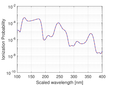
$Z=50$

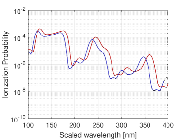
$Z=92$

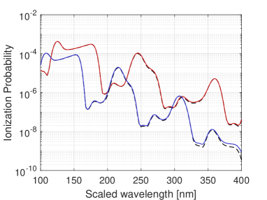
Figure 1: The red curves shows the ionization probability as a functions of the scaled wavelength of the laser pulse for three nuclear charges obtained within the non-relativistic Schrödinger equation. The blue curves are the corresponding relativistic predictions. The black dashed curves are the predictions within the dipole approximation. The upper panel corresponds to hydrogen, $Z=1$, while the middle and lower panels correspond to $Z=50$ and $Z=92$, respectively. The scaled peak electric field strength $\tilde{E}_{0}=0.00955$ a.u..

Figure 1 shows the ionization probability as a function of scaled wavelength calculated in four ways; both the time-dependent Schrödinger and Dirac equations have been solved within the dipole approximation, Eq. (2) and Eq. (3) subject to Eq. (6), and within the long wavelength approximation, Eqs. (7). The ionization probability is strongly non-monotonic due to the onset of resonant transitions via intermediate bound states. For the hydrogen case (top panel), the results of the four calculations are virtually indistinguishable on a logarithmic plot. To a large degree, this is the case for the LWA and the dipole approximation prediction for $Z=50$ as well (middle panel). However, a strong relativistic shift is seen: In general, the predictions from the Dirac equation are somewhat lower in magnitude and shifted significantly towards lower wavelengths compared to the results from the Schrödinger equation. In Ref. Ivanova et al. (2018) this was explained as a consequence of the relativistic shift in the ionization potential.

When it comes to $Z=92$ (lower panel), the contribution from the magnetic field to the ionization probability can indeed be identified – even on a logarithmic scale. It is particularly evident for the Dirac equation at higher wavelengths. The magnetic contribution consistently leads to an increase in the ionization probability as compared to the dipole results.

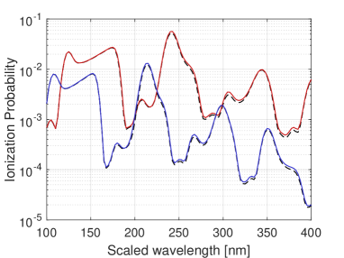
Figure 2: The plot shows the same as the lower panel of Fig. 1, however with an electric field one order of magnitude more intense, $\tilde{E}_{0}=0.03$ a.u..

The same tendency is seen with the higher field intensity. Fig. 2 shows the same as the lower panel of Fig. 1, albeit with a peak electric field strength of $\tilde{E}_{0}=0.03$ a.u.. In this case, magnetic corrections are seen also at lower scaled wavelengths, where the ionization probabilities tend to be higher.

	$\tilde{E}_{0}=0.00955$ a.u.	$\tilde{E}_{0}=0.03$ a.u.
$Z=50$
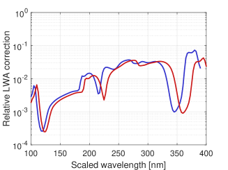
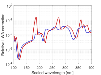
$Z=92$

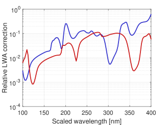
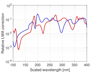
Figure 3: The relative difference in ionization probability between the predictions within the dipole approximation and within the long wavelength approximation (LWA), $(P_{\mathrm{ion}}^{\mathrm{lwa}}-P_{\mathrm{ion}}^{\mathrm{dip}})/P_{\mathrm{ion}}^{\mathrm{lwa}}$, as functions of the scaled wavelength $\tilde{\lambda}$. The blue curves correspond to the Dirac equation, while the red ones correspond to the Schrödinger equation. The nuclear charge $Z=50$ in the upper panels while the lower ones are obtained with $Z=92$. For the left panels, the scaled peak electric field strength $\tilde{E}_{0}=0.00955$ a.u., while $\tilde{E}_{0}=0.03$ a.u. in the right panels.

In order to get a clearer picture of the role of the magnetic correction, we display the difference between the LWA and the dipole predictions in Fig. 3. In the figure, the correction is shown relative to the total (LWA) ionization probability. While the relative correction seems to be about the same order or magnitude for both field strengths, it tends to be larger for higher $Z$, c.f., Eq. (15). The magnetic correction reaches about 10 % for $Z=92$. Also, the relative correction tends to be higher for higher wavelengths, where the ionization probability tends to be lower. These observations can be understood from the fact that the excursion amplitude of a classical non-relativistic free electron in the field scales quadratically with the wavelength, $r_{\mathrm{excur}}=eE_{0}/(4\pi^{2}mc^{2})\,\lambda^{2}$ so that the ratio $r_{\mathrm{excur}}/\lambda=eE_{0}/(4\pi^{2}mc^{2})\,\lambda=Z\,e\tilde{E}_{0}/(4\pi^{2}mc^{2})\,\tilde{\lambda}$. As this ratio increases, so does the influence of the spatial dependence of the vector potential and, thus, also the magnetic interaction.

III.2 Distinguishing dynamical and structural relativistic corrections

As discussed in Sec. II.1, there are two candidates for distinguishing between the relativistic correction originating from the modified spectrum of the ion and that induced by the external field. The Hamiltonians of Eq. (11) account for the increased inertia of the electron accelerated by the laser, they do not, however, consider the fact that the Coulomb potential also may accelerate it towards relativistic speeds. The Hamiltonian of Eq. (13), on the other hand, involves the time-independent part of the Hamiltonian in a fully relativistic manner, while the interaction, which involves ${\bf p}$ instead of the “momentum” $mc\boldsymbol{\alpha}$, is non-relativistic in nature.

	$\tilde{E}_{0}=0.00955$ a.u.	$\tilde{E}_{0}=0.03$ a.u.
$Z=1$
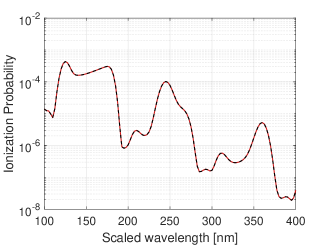
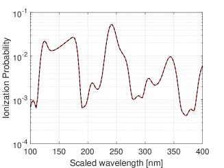
$Z=50$
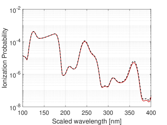
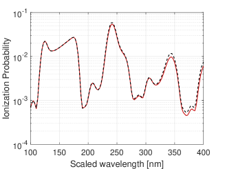
$Z=92$

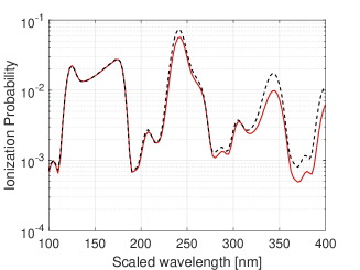
Figure 4: These panels show the semi-relativistic correction to the non-relativistic calculations. The full curves show the ionization probability calculated from the Schrödinger Hamiltonian within the long wavelength approximation, Eq. (7a), while the dashed curves also include the lowest order semi-relativistic correction, Eq. (11b). The panels correspond to, from top to bottom, nuclear charges $Z=1$, $Z=50$ and $Z=92$, the left panels are obtained with $\tilde{E}_{0}=0.00955$ a.u. while the right panels are obtained with $\tilde{E}_{0}=0.03$ a.u..

In Fig. 4 we demonstrate how the non-relativistic calculations are affected by introducing the relativistic mass shift. The results shown are obtained within the long wavelength approximation; a similar shift is seen within the dipole approximation as well. Specifically, the full curves show the ionization probability obtained with Eq. (3), while the dashed curves are found with Eq. (11b). The figure indicates that dynamical relativistic shifts are indeed significant. As expected, we see increased corrections with increasing nuclear charge and increasing field strength. As in the case of magnetic corrections, the relativistic correction is more pronounced for longer wavelengths. Again, these features can be understood from the analogy with a classical free electron in the electric field. The ratio between the maximum quiver velocity of such an electron and the speed of light would be $v_{\mathrm{quiv}}/c=eE_{0}/(2\pi mc^{2})\,\lambda=Z\,e\tilde{E}_{0}/(2\pi mc^{2})\,\tilde{\lambda}$; it is proportional to both $Z$, $\tilde{E}_{0}$ and $\tilde{\lambda}$.

It is, however, less expected that the semi-relativistic interaction shifts the ionization probability upwards. As one would expect the increased inertia of the electron to stabilize the system rather than enhance the ionization, this hardly seems intuitive.

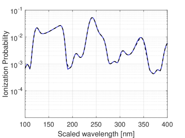
$Z=50$

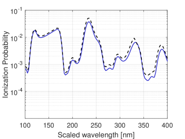
$Z=92$

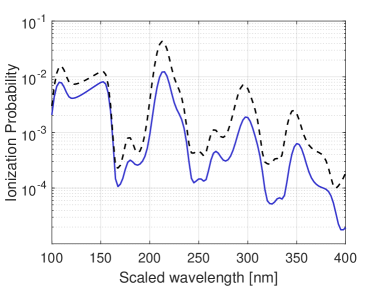
Figure 5: Ionization probability predicted by the Dirac equation within the dipole approximation. The full, blue curve corresponds to the usual minimal coupling Hamiltonian, Eq. (3), while the dashed curve is obtained with the Hamiltonian of Eq. (13), which features a non-relativistic interaction term. The scaled maximum electric field strength is $\tilde{E}_{0}=0.03$ a.u.. The panels correspond to, from top to bottom, nuclear charges $Z=1$, $Z=50$ and $Z=92$.

This observation gives us reason to view this approach with some scepticism. This scepticism is strengthened when we instead compare the prediction of the Dirac equation with the Hamiltonian of Eq. (13) with those of the fully relativistic Dirac Hamiltonian. In Fig. 5 we have shown the ionization probability obtained with the “usual” Dirac Hamiltonian, Eq. (3), and with Eq. (13). In this case, this is done within the dipole approximation. The results are obtained with the higher field intensity, $\tilde{E}_{0}=0.03$ a.u., for the same three nuclear charges as before. As in Fig. 4, we see that the difference between the two calculations increases with $Z$, and with $\tilde{\lambda}$. However, this time the fully relativistic ionization probability is consistently lower than the one obtained with a non-relativistic interaction term.

Although the results of Fig. 4 and 5 both provide clear indications that relativistic corrections induced by the external laser field alone indeed does affect the ionization dynamics, they cannot both provide an adequate description since they predict dynamical relativistic corrections of opposite signs. Two arguments suggest that the positive shift seen in Fig. 4 is erroneous. The first is the fact that it contradicts the expectation that increased inertia would stabilize the system, as discussed above. The second is the fact that the truncation imposed in going from Eq. (8) to Eqs. (11) may be questioned. In principle, the Hamiltonian of Eq. (8) should provide relativistic energies even without any field present – at least in a spin-independent, classical sense. Consequently, the time-independent higher order terms in an expansion of Eq. (8) do provide significant contributions. If we were to retain the full next-to-leading order term in $q^{2}$ in Eq. (8), the semi-relativistic Hamiltonians in Eq. (11) would acquire the additional term $-q^{4}/(8\mu^{3}c^{2})$. In the dipole approximation this term may be written

$$-\frac{q^{4}}{8\mu^{3}c^{2}}=-\frac{p^{4}+4e({\bf A}\cdot{\bf p})p^{2}+4e^{2}({\bf A}\cdot{\bf p})^{2}}{8\mu^{3}c^{2}}.$$ (27)

While the first term in the numerator is a pure structure-correction, the second one, which also appears in the long wavelength approximation, mixes the interaction term ${\bf A}\cdot{\bf p}$ with the time-independent $p^{2}$. While such higher order contributions can typically be neglected for hydrogen in the strong field limit, see Kjellsson Lindblom et al. (2018), these terms may in fact contribute at, comparatively, more moderate fields – also in the X-ray regime Førre (2019). Moreover, the fact that the $-p^{4}/(8m^{3}c^{2})$ structure correction is of increasing importance with increasing $Z$ may indicate that also the other terms in Eq. (27) become significant for highly charged ions.

Interestingly, this also challenges the idea we had from the outset, namely that the relativistic correction can be separated in a structure contribution and a dynamical contribution. This combined effect is likely to impose an effective reduction of the electric interaction $e/m\;{\bf A}\cdot{\bf p}$ – a reduction which increases with increasing $\langle p^{2}\rangle$, which, in turn, increases with $Z$ due to the Coulomb attraction. While it certainly would be interesting to study this effect, this is beyond the scope of the present work.

Motivated by the observation that structural and dynamical relativistic effects mix in the semi-relativistic formulation, we may also question whether this distinction makes sense using the alternative formulation of Eq. (13). However, this formulation comes about by a unitary transformation, Eq. (12), which depends explicitly on the interaction with the external field. Thus, so does all higher order terms beyond those included in Eq. (13). Moreover, as the time-independent part of the Dirac Hamiltonian is left unchanged by the transformation, the structure is still described in a fully relativistic manner. Thus, we do find that the distinction between Eq. (3) and Eq. (13) remains a reasonable measure of laser induced relativistic corrections.

IV Conclusions

We studied photo ionization of hydrogen-like ions exposed to laser fields as a function of laser wavelength. For hydrogen, the calculations where performed with peak intensities corresponding to $3.2\times 10^{12}$ W/cm² and $3.2\times 10^{13}$ W/cm² with wavelengths ranging from the weakly ultra violet region up to the onset of the optical region. For the ions, the laser parameters were scaled such that the ionization probabilities predicted by the time-dependent Schrödinger equation within the dipole approximation were invariant. Thus, deviations from this ionization probability was evidence of either relativistic or magnetic corrections.

By comparing these results with relativistic calculations beyond the dipole approximation, the nature of these corrections was studied. It was confirmed that the increased ionization potential of the ions indeed was the most significant source of relativistic corrections. Moreover, we demonstrated that the magnetic correction is significant – and increasingly so with increasing nuclear charge and scaled wavelength.

Finally, we investigated to what extent some of the relativistic corrections were attributable to the external field alone. Our results provide an affirmative answer to this question. While the magnetic interaction tends to enhance ionization, laser induced relativistic effects tend to stabilize the ion against ionization.

$Z=1$

$Z=1$

References

- Di Piazza et al. (2012) A. Di Piazza, C. Müller, K. Z. Hatsagortsyan, and C. H. Keitel, Rev. Mod. Phys. 84, 1177 (2012).
- Braun et al. (1999) J. W. Braun, Q. Su, and R. Grobe, Phys. Rev. A 59, 604 (1999).
- Fillion-Gourdeau et al. (2012) F. Fillion-Gourdeau, E. Lorin, and A. D. Bandrauk, Comput. Phys. Commun. 183, 1403 (2012).
- Ivanov (2015) I. A. Ivanov, Phys. Rev. A 91, 043410 (2015).
- Fillion-Gourdeau et al. (2016) F. Fillion-Gourdeau, E. Lorin, and A. Bandrauk, J. Comput. Phys. 307, 122 (2016).
- Kjellsson et al. (2017a) T. Kjellsson, S. Selstø, and E. Lindroth, Phys. Rev. A 95, 043403 (2017a).
- Kjellsson et al. (2017b) T. Kjellsson, M. Førre, A. S. Simonsen, S. Selstø, and E. Lindroth, Phys. Rev. A 96, 023426 (2017b).
- Ivanova et al. (2018) I. V. Ivanova, V. M. Shabaev, D. A. Telnov, and A. Saenz, Phys. Rev. A 98, 063402 (2018).
- Kjellsson Lindblom et al. (2018) T. Kjellsson Lindblom, M. Førre, E. Lindroth, and S. Selstø, Phys. Rev. Lett. 121, 253202 (2018).
- Fillion-Gourdeau et al. (2017) F. Fillion-Gourdeau, S. MacLean, and R. Laflamme, Phys. Rev. A 95, 042343 (2017).
- Blanes et al. (2009) S. Blanes, F. Casas, J. Oteo, and J. Ros, Physics Reports 470, 151 (2009).
- Selstø et al. (2009) S. Selstø, E. Lindroth, and J. Bengtsson, Phys. Rev. A 79, 043418 (2009).
- Vázquez de Aldana et al. (2001) J. R. Vázquez de Aldana, N. J. Kylstra, L. Roso, P. L. Knight, A. Patel, and R. A. Worthington, Phys. Rev. A 64, 013411 (2001).
- Førre and Simonsen (2016) M. Førre and A. S. Simonsen, Phys. Rev. A 93, 013423 (2016).
- Simonsen and Førre (2016) A. S. Simonsen and M. Førre, Phys. Rev. A 93, 063425 (2016).
- Sonnleitner and Barnett (2018) M. Sonnleitner and S. M. Barnett, Phys. Rev. A 98, 042106 (2018).
- Reiss (1979) H. R. Reiss, Phys. Rev. A 19, 1140 (1979).
- Sarachik and Schappert (1970) E. S. Sarachik and G. T. Schappert, Phys. Rev. D 1, 2738 (1970).
- Førre (2019) M. Førre, Phys. Rev. A 99, 053410 (2019).
- Foldy and Wouthuysen (1950) L. L. Foldy and S. A. Wouthuysen, Phys. Rev. 78, 29 (1950).
- Madsen and Lambropoulos (1999) L. B. Madsen and P. Lambropoulos, Phys. Rev. A 59, 4574 (1999).
- deBoor (1978) C. deBoor, A Practical Guide to Splines (Springer-Verlag, New York, 1978).
- Fischer and Zatsarinny (2009) C. F. Fischer and O. Zatsarinny, Comput. Phys. Commun. 180, 879 (2009).
- Vanne and Saenz (2012) Y. V. Vanne and A. Saenz, Phys. Rev. A 85, 033411 (2012).
- Saad (1992) Y. Saad, SIAM J. Numer. Anal. 29, 209 (1992).