Academic Performance Estimation with Attention-based Graph Convolutional Networks

Abstract

Student’s academic performance prediction empowers educational technologies including academic trajectory and degree planning, course recommender systems, early warning and advising systems. Given a student’s past data (such as grades in prior courses), the task of student’s performance prediction is to predict a student’s grades in future courses. Academic programs are structured in a way that prior courses lay the foundation for future courses. The knowledge required by courses is obtained by taking multiple prior courses, which exhibits complex relationships modeled by graph structures. Traditional methods for student’s performance prediction usually neglect the underlying relationships between multiple courses; and how students acquire knowledge across them. In addition, traditional methods do not provide interpretation for predictions needed for decision making. In this work, we propose a novel attention-based graph convolutional networks model for student’s performance prediction. We conduct extensive experiments on a real-world dataset obtained from a large public university. The experimental results show that our proposed model outperforms state-of-the-art approaches in terms of grade prediction. The proposed model also shows strong accuracy in identifying students who are at-risk of failing or dropping out so that timely intervention and feedback can be provided to the student.

1 Introduction

Higher educational institutions face major challenges including timely graduation and retention of enrolled students. The National Center for Education Statistics (NCES) reports that the six-year graduation rate for first-time and full-time undergraduates is around 60%; the retention rate among first-time and full-time degree-seeking students is around 80% [1]. These alarming statistics require higher educational institutions to take actions to improve their effectiveness and efficiency at educating students. Machine learning techniques have been increasingly developed and applied to educational settings in the hope of improving students’ learning and increasing students’ success [3, 26, 16]. Many systems and applications have been proposed; such as course recommender systems [7], academic trajectory and degree planning [20], educational early advising systems [9], and knowledge tracing for intelligent tutoring systems [35, 22]. Developing methods for accurate modeling and predicting students’ performance is the key to these systems and applications.

Traditional performance prediction methods can be categorized into two types. The first builds a static model, which takes a feature vector as input (such as a student’s grades in previous courses or student-related features) and outputs the predicted grades. A common approach that belongs to this category is linear regression methods [23]. Students take courses sequentially, i.e., they take some courses at each semester; and their performance in courses taken in the next semester depends on courses taken in previous semesters. Further, their knowledge evolves by taking a sequence of courses. To capture the temporal dynamics of students’ knowledge evolution, sequential models have been proposed. A set of representative approaches within this category use recurrent neural networks (RNN) [12, 11].

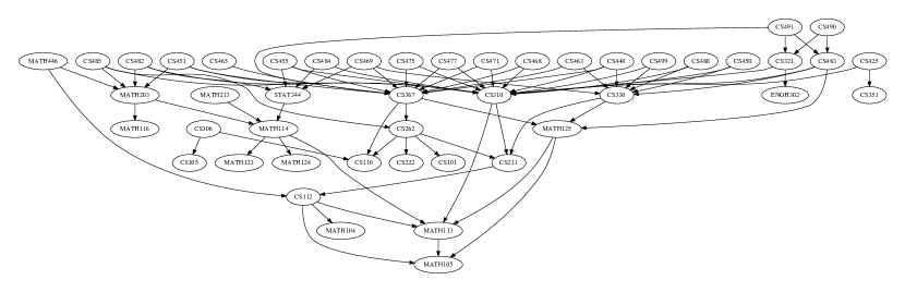
(a) Computer Science

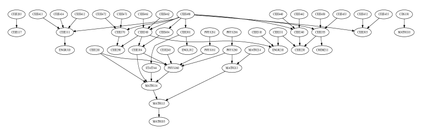
(b) Civil Engineering

Figure 1: Course dependence structure in two representative majors.

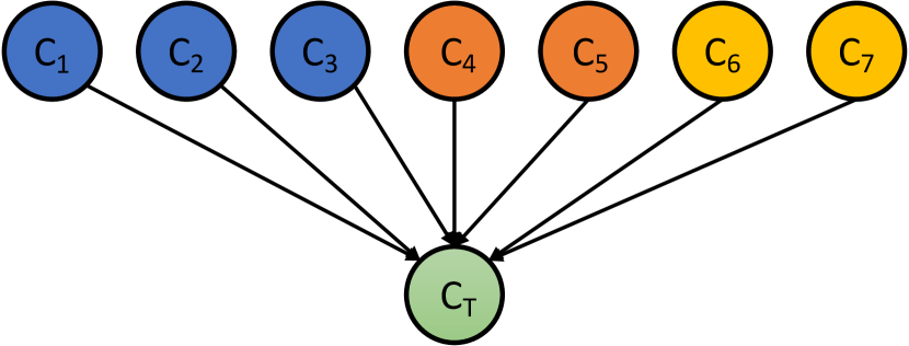
(a) Static Model

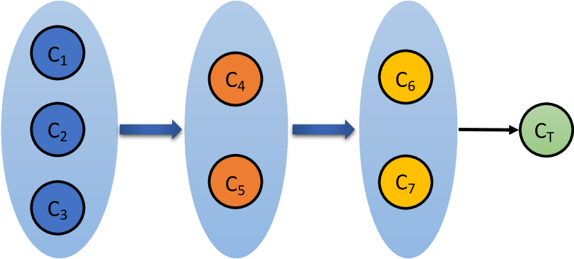
(b) Sequential Model

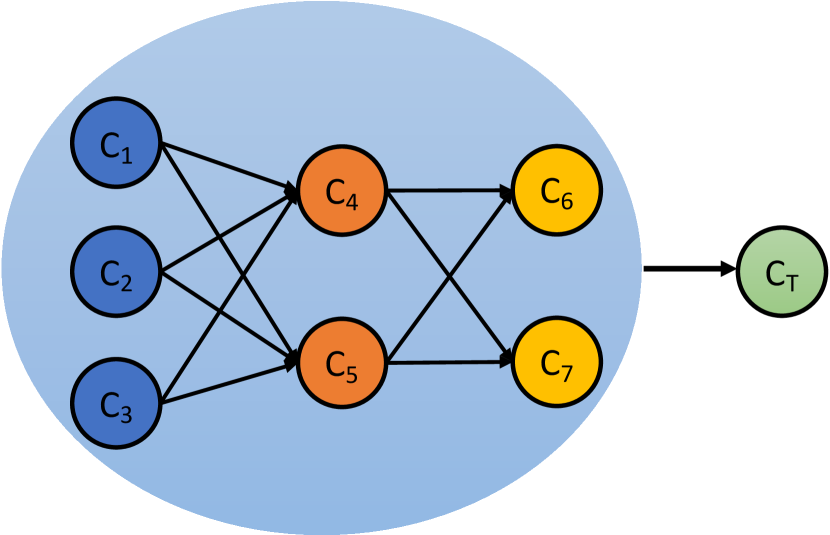
(c) Graph Model

Figure 2: Comparison of Three Types of Model Architectures. In this example, a student takes course $C_{1},C_{2},C_{3}$ in the first semester, course $C_{4},C_{5}$ in the second semester, course $C_{6},C_{7}$ in the third semester before takes the target course $C_{T}$.

Undergraduate degree programs are designed in a way that knowledge acquired in prior courses serves as prerequisites for future courses. The knowledge and skills required to do well in a course are acquired in multiple prior courses. The knowledge dependence between courses exhibit complex graph structure as shown in Figure 1. Figure 1 shows the prerequisite structures for computer science and civil and infrastructure engineering degree programs at George Mason University. Each node represents a particular course. An edge pointing from one course to another shows the prerequisite relationship. As an example, to do well in the data structure course (CS310), students need to acquire programming skills, object-oriented programming knowledge (CS211) and math (MATH113) which come from multiple different courses. The graph in Figure 1 also shows hierarchical relationships where a course can depend on another course which is at a much lower academic level. In addition to the prerequisite structures, degree programs are flexible, i.e., students can choose to take elective courses based on their interests and do not have to follow a specific ordering when taking these courses.

The complexity and flexibility of the degree programs make predicting students’ performance a challenge task. Prior approaches usually simplify or ignore these complex dependencies. Figure 2 shows the comparison of three types of models. Figure 2(a) shows a static model, where a student’s performance is directly dependent on a set of prior courses. Figure 2(b) shows a sequential model, where students’ knowledge evolution is partially modeled. To overcome the constraints and limitations of the traditional models, we propose a model based on graph convolutional networks to capture the complex graph-structured knowledge evolution exhibited by students’ data. Specifically, we propose an attention-based graph convolutional network (ACGN) model for predicting a student’s grade in a future course. Figure 2(c) shows the graph model, where each course depends on all courses taken in the semester before it so that students’ knowledge evolution is fully captured.

When a system is used for decision making e.g., as a support tool for advisors to identify students who are at-risk of failing courses they will take; it is essential for the predictions to be interpretable. This allows the stakeholders to trust the decision making systems and make informed decisions. We show that our attention-based model is able to provide an interpretable and useful explanation for the predictions. Our model is able to analyze a student’s performance in prior courses and identify a collection of important prior courses to explain the student’s performance in target course.

We performed extensive experiments on real-world datasets to evaluate our model and compare it with the other two types of models aforementioned. The experimental results are consistent with our observations that models with architectures more close to the degree program have better modeling capability and prediction performance. One of the important applications for students’ performance prediction is early warning and advising systems, where at-risk students are first identified and timely support is provided to improve their academic success. The experimental results show our model’s effectiveness at identifying at-risk students.

The key contributions of the paper are summarized as follows:

• Flexible graph structured model for students’ academic performance prediction. Observing the complex structures of undergraduate degree programs, we propose a graph convolutional network model for students’ performance prediction.

• Attention based model for explanation. Providing explanations for a model’s predictions makes the model useful for decision making. Our attention-based model can explain the predictions by identifying a set of prior courses important for the predictions.

• Identification of at-risk students. While most models achieve good performance at predicting students’ performance, they suffer from low accuracy at identifying at-risk students. Our proposed model is able to achieve comparable performance with state-of-the-art models.

2 Related Work

The need to improve higher education services and offerings has attracted research on developing methods for predicting students’ performance [4, 27]. In this section, we review related work on students’ performance prediction. The related work can be classified into three categories: (i) static models, (ii) sequential models and (iii) graph models.

2.1 Static Models

Static grade prediction models learn a mapping function, where input is student-related features and the output is predicted grade. Polyzou et al. [23] proposed regression models specific to courses or students for predicting a student’s grade in a target course. They found that focusing on a course specific subset of the data leads to more accurate predictions. Elbadrawy et al. [8] introduced a personalized multi-regression model for predicting students’ performance in course activities. Compared to a single regression model, this model is able to capture personal student differences. To understand how students’ behavior impacts their academic performance, Wang et al. [32] collects students’ behavioral data using smart phone for performance prediction. Many other classic supervised learning approaches have been used for students’ performance prediction including decision trees [2], support vector machines and neural networks [31].

Adapted from recommender systems domain, matrix factorization [14] approaches are popular for grade prediction. These factorization approaches make the assumption that a student’s knowledge/skills and a course’s knowledge components can be jointly represented with latent vectors (factors) [30]. Polyzou et al. [23] proposed course-specific matrix factorization models for grade prediction that decompose a course-specific subset of students’ grade data. The student course records also exhibit grouping structures and a domain-aware matrix factorization model was developed for the joint course recommendation and grade prediction [7]. Ren et al. [25] proposed matrix factorization model coupled with temporal dynamics for grade prediction.

2.2 Sequential Models

Students take courses sequentially. Their knowledge and skills evolve by taking a series of courses. To model the temporal dynamics of students’ knowledge evolution, sequential models have been proposed. Balakrishnan [5] proposed a Hidden Markov Model for predicting student dropout by modeling students’ activities over time in a Massive Open Online Courses (MOOCs). Swamy et al. [29] models student progress on coding assignments in large-scale computer science courses using recurrent neural networks. Kim et al. [12] proposed a bidirectional long short term memory (BLSTM) model for the online educational setting. Hu et al. proposed course-specific markovian models for students’ grade predictions [10]. Morsy et al. proposed cumulative knowledge-based regression models for next-term grade prediction, which models students’ knowledge evolution by using a sequential regression model. Hu et al. [11] proposed long short term memory models for grade prediction in traditional higher education.

2.3 Graph Neural Networks Models

Deep learning approaches have found unprecedented success in a myriad of applications involving regular structured data such as images (grids) and text (sequences) [18]. Graphs are more complex and irregular than grids or sequences and recent research efforts involve designing deep learning models for graph data. Graph neural networks have been proposed and applied to many areas such as computer vision for point clouds classification [33], action recognition [34]; recommender systems [6] and traffic prediction [19]. To the best of our knowledge, there is no prior work on students’ performance prediction using graph neural networks.

3 Methods

3.1 Problem Statement

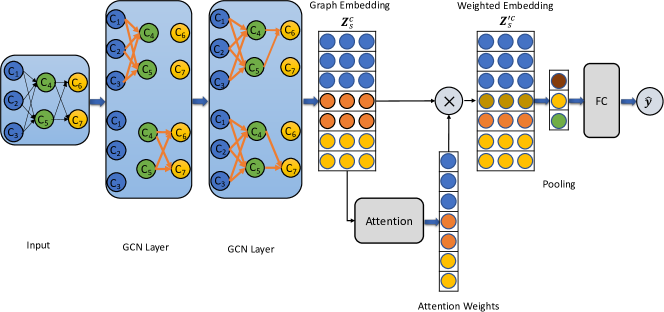
Figure 3: The proposed model.

Given a student $s$, the set of courses taken and grades obtained in term $t$ are represented by $\mathbb{P}_{s}^{t}$. For a sequence of terms $1\ldots T_{s}$, we denote $\mathbb{P}_{s}^{1\sim T_{s}}=\mathbb{P}_{s}^{1},\mathbb{P}_{s}^{2},\ldots,\mathbb{P}_{s}^{T_{s}}$ to represent the sequence of courses taken and grades obtained by student $s$ in $T_{s}$ terms. For a target course $c$ taken in the future (next) term, the objective of the proposed method is to predict the grade student $s$ will achieve in course $c$ denoted by $\hat{g}_{s}^{c}$.

The proposed models are trained in a course specific manner i.e., for each target course $c$ we learn a unique model. Due to the flexibility of academic degree programs, in each semester different courses can be taken; and for each student, the number of semesters studied before taking the target course will be different. Therefore, we index the length of the sequence with student-specific variable $T_{s}$.

For every target course $c$, a subset of frequently taken prior courses are identified from all the prior courses taken by students who have already taken the target course $c$. These prior courses are denoted as $\mathbb{C}_{c}$ of size $N_{c}$. For student $s$, only the prior courses in $\mathbb{C}_{c}$ are extracted from $\mathbb{P}_{s}^{1\sim T_{s}}$ to form a graph which is represented by an adjacency matrix $\mathbf{A}_{s}^{c}\in\{1,0\}^{N_{c}\times N_{c}}$ and a feature matrix $\mathbf{F}_{s}^{c}\in\mathbb{R}^{N_{c}\times D}$, where $D$ represents the number of features. Take Figure 2(c) as an example, the student takes courses $c_{1},c_{2},c_{3}$ in the first term, $c_{4},c_{5}$ in the second term and $c_{6},c_{7}$ in the third term; we want to predict his/her grade in course $C_{T}$. Adjacency matrix $\mathbf{A}_{s}^{c}$ for this student represents his course taken process. Courses taken in the current term are fully connected to courses taken in the next term; 1 represents connected, 0 otherwise. A row of the feature matrix $\mathbf{F}_{s}^{c}$ represents the student’s grades in corresponding prior courses.

3.2 Model Description

Figure 3 shows an overview of the proposed model. It is composed of three parts: 1) graph convolutional network, 2) attention layer and 3) a fully connected layer.

3.2.1 Graph Convolutional Network (GCN)

Convolutional neural networks (CNNs) show superior performance on several applications related to vision [15], speech and text [17]. CNNs are powerful because of their ability to exploit feature locality at multiple granularity. Graph Convolutional networks have a similar working mechanism but on data with more complex structures, namely, graph.

The input to a GCN is an adjacency matrix $\mathbf{A}_{s}^{c}$ and feature matrix $\mathbf{F}_{s}^{c}$, encoding student $s$’s course taking process and grades in prior courses, respectively. Multiple layers of graph convolutional layer are applied on $\mathbf{A}_{s}^{c}$ and $\mathbf{F}_{s}^{c}$ to learn a graph level embedding $\mathbf{Z}_{s}^{c}\in\mathbb{R}^{N\times D}$. Each row of $\mathbf{Z}_{s}^{c}$ corresponds to a node embedding vector. A graph convolutional layer is mathematically described as follows:

$$\mathbf{H}^{(l+1)}=f(\mathbf{H}^{(l)},\mathbf{A})=\sigma(\tilde{\mathbf{D}}^{-\frac{1}{2}}\tilde{\mathbf{A}}\tilde{\mathbf{D}}^{-\frac{1}{2}}\mathbf{H}^{(l)}\mathbf{W}^{(l)})$$ (1)

where $\tilde{\mathbf{A}}=\mathbf{A}+\mathbf{I}_{N}$ is the adjacency matrix with self-connections, $\tilde{\mathbf{D}}=\Sigma_{j}\tilde{\mathbf{A}}_{j}$ is the normalization matrix, $\mathbf{H}^{(l)}$ is the input and $\mathbf{W}^{(l)}$ is the weight matrix to be learned. $\mathbf{H}^{(0)}=\mathbf{F}_{s}^{c}$ and $\mathbf{H}^{(L)}=\mathbf{Z}_{s}^{c}$; namely, the input into the first GCN layer is the feature matrix $\mathbf{F}_{s}^{c}$, the output from the last GCN layer is the student-specific graph embedding $\mathbf{Z}_{s}^{c}$.

A filter in convolutional neural networks aggregates information from a pixel’s neighbors. Similarly, the graph convolutional layer aggregates information from a node’s neighboring nodes and generates a new node embedding vector by the following equation

$$\mathbf{h}_{i}=\sigma(\Sigma_{j}\frac{1}{c_{ij}}\mathbf{h}_{j}\mathbf{W})$$ (2)

where node $j$ is node $i$’s neighbor. A higher level of the node embeddings are generated by applying multiple GCN layers. Multiple layers of GCN aggregate information from a node’s further neighbors. As shown in Figure 3, the first GCN layer aggregates information from a node’s direct neighbors, namely, in our case the courses taken in last semester. The second layer collects information from a node’s second degree neighbors, i.e., the courses taken two semesters ago. The final output is the graph embedding which entails information from all the courses a student has taken.

3.2.2 Attention Layer

The output from GCNs is a graph-level embedding matrix, which encodes information about a student’s knowledge and skills acquired in prior courses. The knowledge acquired from different prior courses has different importance for the target course. To capture the importance differences of the prior courses, we integrate attention layer into our model. Attention mechanism allows the model to focus on the relevant features or information useful for prediction. It works by computing an importance score [24], higher score means the corresponding prior course is more important for predicting a student’s performance; given by

$$e_{i}=MLP(\mathbf{h}_{i})$$ (3)

$$\alpha_{i}=\frac{\exp(e_{i})}{\Sigma_{k=1}^{N}\exp(e_{k})}$$ (4)

where $MLP$ is a learnable function, i.e., multi-layer perceptron, $\alpha_{i}$ is the attention score corresponds to $\mathbf{h}_{i}$. The output from the attention layer is an attention score vector $\bm{{\alpha}}$.

The graph embedding matrix $\mathbf{Z}_{s}^{c}$ is weighted by attention scores to form a weighted graph embedding matrix $\mathbf{Z}_{s}^{{}^{\prime}c}$ given by

$$\mathbf{Z}_{s}^{{}^{\prime}c}=\begin{bmatrix}{1}&\alpha_{1}\mathbf{z}_{s,1}^{c}&{1}\\ &\vdots&\\ {1}&\alpha_{i}\mathbf{z}_{s,i}^{c}&{1}\\ &\vdots&\\ {1}&\alpha_{N}\mathbf{z}_{s,N}^{c}&{1}\\ \end{bmatrix}$$ (5)

Finally, the pooling layer coarsens the weighted graph embedding matrix into a latent vector $\mathbf{v}_{s}^{c}$. The latent vector is passed through a multilayer perceptron; the output from which is the predicted grade.

$$\hat{g}_{s}^{c}=f(\mathbf{v}_{s}^{c})$$ (6)

where $f$ is a multilayer perceptron network.

4 Experimental Protocol

4.1 Dataset Description

Table 1: Dataset Statistics

Major Fall 2017 Spring 2018 #S #C #G #S #C #G CS 5,042 16 47,889 5,297 20 52,152 ECE 1,992 18 34,355 1,980 18 34,170 BIOL 7,065 20 52,574 6,976 20 52,672 PSYC 5,367 20 25,207 5,368 20 25,247 CEIE 2,222 17 30,956 2,181 16 30,283 Overall 21,688 91 190,981 21,802 94 194,524 • #S total number of students, #C number of courses for prediction, #G total number of grades

The data is collected at George Mason University from Fall 2009 to Spring 2018. The five largest majors are chosen including: 1) Computer Science (CS), 2) Electrical and Computer Engineering (ECE), 3) Biology (BIOL), 4) Psychology (PSYC) 5) Civil Engineering (CEIE). The evaluation procedure is designed in a way to simulate the real-world scenario of predicting the next-term grades. Specifically, the models are trained on the data up to term $T-2$ and validated on term $T-1$ and tested on term $T$. The latest two terms are chosen as testing terms, i.e. term Fall 2017 and term Spring 2018. For example, to evaluate the performance of the models on term Fall 2017, the model is trained on data from term Fall 2009 to term Fall 2016, validated on term Spring 2017 to choose the parameters associated with different approaches and finally tested in term Fall 2017. The statistics of the datasets are listed in Table 1

4.2 Evaluation Metrics

We evaluate the models from two perspectives: 1) the accuracy of grade predictions, 2) the models’ ability at detecting at-risk students.

To evaluate the models’ accuracy of grade prediction, two evaluation metrics are used a) mean absolute error (MAE) and b) percentage of tick accuracy (PTA).

$$\text{MAE}=\frac{\sum_{i=1}^{N}{|g_{i}-\hat{g}_{i}}|}{N}$$ (7)

where $g_{i}$ is true grade and $\hat{g}_{i}$ is predicted grade.

In the grading system, there are 11 letter grades (A+, A, A-, B+, B, B-, C+, C, C-, D, F) which correspond to (4, 4, 3.67, 3.33, 3, 2.67, 2.33, 2, 1.67, 1, 0). A tick is the difference between two consecutive letter grades. The performance of a model is estimated by how many ticks away the predicted grade is from the true grade. For example, the tick error between B and B is zero, B and B+ is one, B and A- is two. To use PTA for evaluation, we first convert the predicted numerical grade to its closest letter grade and then compute the percentage of errors with 0 tick, within 1 tick, and within 2 ticks denoted by PTA₀, PTA₁, and PTA₃, respectively.

We also evaluate the models’ performance of identifying at-risk students. At-risk students are defined as those whose grades are lower than 2.0 (C, C-, D, F). The predicted grades below 2.0 are treated as positives and above 2.0 are treated as negatives. The process of detecting at-risk students is similar to grade prediction except that the output from the model (the predicted grade) is converted to 1 or 0 based on whether the predicted grade is below or above 2.0. As the number of at-risk students is low, we use F-1 score as evaluation metric.

4.3 Comparative Methods

Bias Only (BO)

Bias only method only takes into account a student’s bias, a course’s bias and global bias[23]. The predicted grade is as follow

$$\hat{g}_{s}^{c}=b^{c}+b_{s}^{c}+b_{c^{\prime}}^{c}$$ (8)

where $b^{c},b_{s}^{c},b_{c^{\prime}}^{c}$ are global bias, student bias and course bias, respectively.

Course Specific Matrix Factorization (CSMF)

The key assumption underlying this model is that students and courses can be jointly represented by low-dimensional latent factors. $N$, $M$ and $D$ is the number of students, courses and latent dimension, respectively [23]. To predict a student’s grade in a course, we have:

$$\hat{g}_{s}^{c}=b^{c}+b_{s}^{c}+b_{c^{\prime}}^{c}+<\mathbf{u}_{s}^{c},\mathbf{v}_{c^{\prime}}^{c}>$$ (9)

where $b^{c}$ is global bias, $b_{s}^{c}$ is student bias term, $b_{c^{\prime}}^{c}$ is course bias term; $\mathbf{u}_{s}^{c}$ is student $s$’s latent vector, $\mathbf{v}_{c^{\prime}}^{c}$ is course $c$’s latent vector.

Course Specific Regression (CSR)

Course specific regression (CSR) [23] is a linear regression model. The input into this model is a vector $\mathbf{x}_{s}^{c}$ representing a student’s grades in prior courses. A course specific subset of prior courses included in $\mathbb{P}_{s}^{1\sim T_{s}}$ are flattened to form the vector $\mathbf{x}_{s}^{c}$. The predicted grade is

$$\hat{g}_{s}^{c}=w_{0}^{c}+\mathbf{x}_{s}^{c}\mathbf{w}^{c}$$ (10)

where $w_{0}^{c}$ is bias term and $\mathbf{w}^{c}$ are weight vectors to be learned.

Multilayer Perceptron (MLP)

Multilayer Perceptron is a generalized version of CSR. CSR model is a linear model, which is not able to capture non-linear and complex patterns in students’ grades data. Therefore, multilayer perceptron has been proposed by [11] for grade prediction. Similar to CSR, the input $\mathbf{x}_{s}^{c}$ is a student’s grades in prior courses.

$$\hat{g}_{s}^{c}=f(\mathbf{x}_{s}^{c})$$ (11)

where $f$ is the model to be learned.

Long Short Term Memory (LSTM)

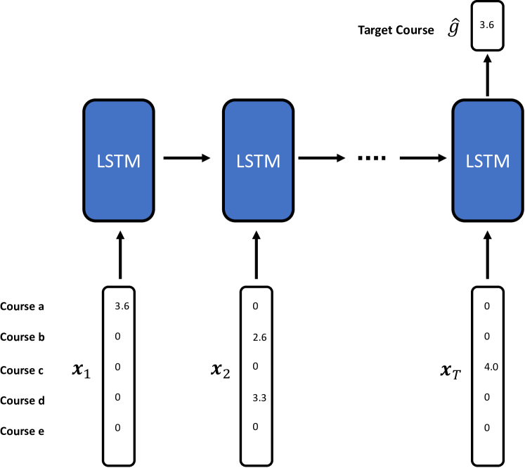
Figure 4: LSTM for grade prediction

Long short term memory (LSTM) is an extension of recurrent neural networks (RNN) for modeling sequential data. The assumption of using LSTM for students’ performance prediction is that students knowledge and skills are evolving by taking courses in each semester. To capture the temporal dynamics of students’ knowledge evolution, LSTMs have been proposed in [11]. The input $\mathbf{x}_{s,t}^{c}$ at time step $t$ is a student’s grades in courses at semester $t$. Many to one architecture is utilized and the output from the last step of LSTM is fed into a fully connected network; the output from which is the predicted grade. The model architecture is shown in Figure 4, where the courses $a,b,c,d,e$ are prior courses, $\mathbf{x}_{s,t}^{c}$ encodes the student’s grades in courses at time $t$ and the output $\hat{g}$ is the predicted grade.

4.4 Implementation

Our method is implemented in Pytorch [21]. For model optimization we use Adam [13]. To avoid model overfitting, we used $l_{2}$ norm regularization (with coefficient 0.001) and dropout (dropout rate 0.05) [28]. The number of dimensions for the graph embedding is chosen from a list of (8, 12, 16, 20, 32, 64).

5 Experimental Results

5.1 Grade Prediction

Table 2: Comparative Performance of Different Models by MAE. ($\downarrow$ is better)

Method Fall 2017 Spring 2018 CS ECE BIOL PSYC CEIE CS ECE BIOL PSYC CEIE BO 0.684 0.570 0.705 0.556 0.616 0.727 0.674 0.628 0.552 0.605 CSMF 0.594 0.476 0.550 0.517 0.479 0.647 0.539 0.499 0.492 0.491 CSR 0.607 0.444 0.551 0.440 0.441 0.628 0.493 0.463 0.439 0.444 MLP 0.585 0.390 0.515 0.407 0.413 0.590 0.436 0.417 0.413 0.369 LSTM 0.582 0.365 0.532 0.380 0.309 0.590 0.370 0.435 0.356 0.251 AGCN 0.540 0.335 0.459 0.309 0.336 0.543 0.366 0.379 0.316 0.258

Table 3: Comparative Performance of Different Models by Percentage of Tick Accuracy ($\uparrow$ is better)

Fall 2017 Spring 2018 Method CS ECE BIOL PSYC CEIE CS ECE BIOL PSYC CEIE $\text{PTA}_{0}$ BO 16.76 20.75 14.40 15.52 14.90 16.07 12.11 15.42 13.65 19.79 CSMF 20.00 23.58 22.40 23.10 28.85 22.31 17.37 23.35 28.41 28.65 CSR 24.26 33.96 27.60 38.97 40.87 26.29 28.42 34.14 41.33 35.42 MLP 26.32 39.62 31.00 41.72 41.35 27.76 33.68 41.41 43.17 42.19 LSTM 27.21 42.92 37.40 48.62 49.52 30.54 54.74 42.73 49.82 57.29 AGCN 30.00 41.51 38.80 56.21 50.00 36.52 39.47 44.49 50.55 56.77 $\text{PTA}_{1}$ BO 44.71 49.06 43.20 57.59 48.56 44.09 37.37 46.70 57.20 50.00 CSMF 55.15 62.26 60.00 63.10 62.98 52.72 54.74 63.66 59.04 61.98 CSR 55.29 66.04 59.40 66.21 71.63 57.37 63.68 66.30 65.31 69.27 MLP 56.91 69.81 62.80 69.66 74.52 60.03 68.42 68.28 69.37 76.04 LSTM 58.24 73.11 61.40 73.79 79.33 59.10 72.11 72.03 75.65 82.81 AGCN 62.21 75.47 70.00 77.93 79.81 63.61 77.89 74.89 77.86 84.90 $\text{PTA}_{2}$ BO 72.94 81.13 72.40 84.83 81.25 73.97 74.21 77.75 87.45 79.17 CSMF 80.00 86.79 83.60 83.45 87.50 75.30 84.21 84.36 85.24 84.38 CSR 76.76 86.32 80.80 83.45 84.62 77.03 82.63 84.58 82.66 86.46 MLP 79.85 89.62 82.80 85.86 86.54 79.42 86.32 86.34 84.13 90.62 LSTM 77.35 86.79 79.20 84.83 90.87 77.69 83.16 84.58 89.67 91.67 AGCN 81.47 92.45 85.60 88.62 91.83 80.21 88.95 87.67 88.93 93.23

Table 2 reports the performance of ACGN and comparative approaches for the task of next-term grade prediction for the Fall 2017 and Spring 2018 semesters using the MAE metric. The proposed ACGN model achieves the best performance in most cases except the Civil Engineering (CEIE) major. The CEIE major has relatively simpler knowledge dependence structure as shown in Figure 1(b). A majority of higher level courses, such as 300 and 400 level courses for the CEIE major have shallow knowledge dependence. While for CS major, the higher level courses have deeper knowledge dependence or longer pre-requisite chains.

Another observation is that models which are able to capture the complex knowledge dependence more have better performance. The static models (BO, CSMF, CSR, MLP) are outperformed by sequential model (LSTM) in most cases, on average by 9.2%; the sequential model is outperformed by graph model (AGCN), besides CEIE major, on average by 7.0%. The experimental results are consistent with our assumption that the knowledge dependence in the undergraduate degree programs is complexly networked structures and a graph model is well-suited at capturing the underlying dynamics.

Table 3 shows the comparative performance using the percentage of tick error accuracy. In contrast to MAE, the PTA metric can provide a fine-grained view of the errors made by different methods. From Table 3 we observe that the performance gap between models at $\text{PTA}_{0}$ is larger than at $\text{PTA}_{2}$. For example, for CS majors in Fall 2017, the gap between the best performing model AGCN and the worst performing model BO at $\text{PTA}_{0}$ is 13.24%, which is larger than 8.53% at $\text{PTA}_{2}$.

Table 4: Predictive Performance at Identifying At-risk Students, F-1 Score ($\uparrow$ is better)

Method Fall 2017 Spring 2018 CS ECE BIOL PSYC CEIE CS ECE BIOL PSYC CEIE BO 0.092 0.000 0.116 0.000 0.000 0.085 0.000 0.194 0.000 0.000 CSMF 0.385 0.415 0.585 0.154 0.429 0.349 0.291 0.620 0.364 0.526 CSR 0.398 0.514 0.649 0.438 0.490 0.500 0.543 0.623 0.429 0.450 MLP 0.383 0.426 0.630 0.438 0.500 0.534 0.472 0.676 0.400 0.605 LSTM 0.492 0.533 0.553 0.276 0.702 0.584 0.650 0.638 0.400 0.681 AGCN 0.516 0.500 0.660 0.438 0.615 0.594 0.571 0.685 0.483 0.550 • The percentage of at-risk students for each major in Fall 2017 is CS (23.7%), ECE (18.9%), BIOL (25.8%), PSYC (8.3%), CEIE (15.9%); In Spring 2018, it is CS (23.7%), ECE (24.7%), BIOL (18.1%), PSYC (6.6%), CEIE (14.1%).

5.2 Detecting At-risk Students

Detecting at-risk students early is a fundamental task for early warning and advising systems. We evaluate the models’ performance at detecting at-risk students. Table 4 shows the experimental results evaluated by F-1 score. The percentages of at-risk students in different majors are presented at the table footnote. The PSYC major has the lowest percentage of at-risk students. The experimental results show that LSTM and AGCN achieve the best performance at detecting at-risk students. BO performs worst at the detection of at-risk students. BO only captures the average performance of a student and a course, which is biased by other students and courses’ performance and the average performance of other students and courses is usually higher than 2.0 (the threshold of defining at-risk students).

5.3 Interpretation with Attention

Table 5: Case Studies By Attention Score

Target Course True Grade Predicted Grade Prior Courses Grades Attention Score CS-310 F C- MATH-213 N 0.33 MATH-125 N 0.33 CS-262 N 0.33 CS-211 C 0.01 CS-310 D D MATH-213 F 0.913 MATH-114 C 0.072 CS-211 N 0.015 BIOL-311 F C BIOL-213 C+ 0.5315 BIOL-214 C+ 0.4685 BIOL-452 D C CHEM-211 C+ 0.5271 BIOL-214 B 0.2784 BIOL-213 C 0.1945 • N means that the student did not take the course. Courses in bold mean they are in prerequisites chain.

Machine learning models have achieved impressive performance in many tasks. However, most of them remain black boxes and there are concerns about their transparency. A model’s capability to provide explanations for its predictions can increase its transparency. For decision making, understanding the reasons behind predictions can help decision makers make informed decisions. Grade prediction models serve as an assistant tool for advisors to make decisions on whether to intervene on a student or not. When the model predicts that a student is at-risk of failing a course, knowing which prior courses results in the prediction can also help advisors provide personalized feedback to students.

Attention mechanism works by letting the model focus on important information for prediction. In our proposed model, the design of the attention layer lets the model focus on important prior courses. The output from the attention layer is a vector of scores representing the importance of the prior courses computed by Equation 4. In this section, we show by case studies how the attention scores from the attention layer explain the model’s predictions, especially, why the model predicts that a student is at-risk of failing a target course.

Table 5 shows four case studies. We keep the most important prior courses identified by attention score. For the first case study, the target course is CS-310, the student’s true grade in the target course is F and the predicted grade is C-. The most important four courses identified by attention layer is MATH-212, MATH-125, CS-262, CS-211. The reason for predicting this student as at-risk is that the student did not take MATH-212, MATH-125, CS-262, therefore lacks the necessary knowledge to do well in the target course. In the second case, the student’s true grade in CS-310 is D, the predicted grade is D. The three most important courses are MATH-213, MATH-114, CS-211. The reason for predicting this student as failing the target course is that he failed MATH-213 and did not do well in MATH-114 and did not take CS-211, which is the prerequisite of the target course. In the third case, the student’s true grade in the target course is F and the predicted grade is C. The two most important prior courses identified are BIOL-213 and BIOL-214, both are in prerequisite chain of the target course and the student did not do well in them. The fourth case shows that the student failed the target course BIOL-452 and the predicted grade is C. The three most influential prior courses are CHEM-211, BIOL-214, BIOL-213. Courses CHEM-211 and BIOL-213 are in prerequisite chain and the student did not perform well in them.

From the case studies, we can see that the attention layer identifies missing knowledge components for a target course, arising due to two reasons: 1) the student did not take some important prior courses, 2) the student did not do well in the corresponding prior courses.

5.4 Sensitivity Analysis

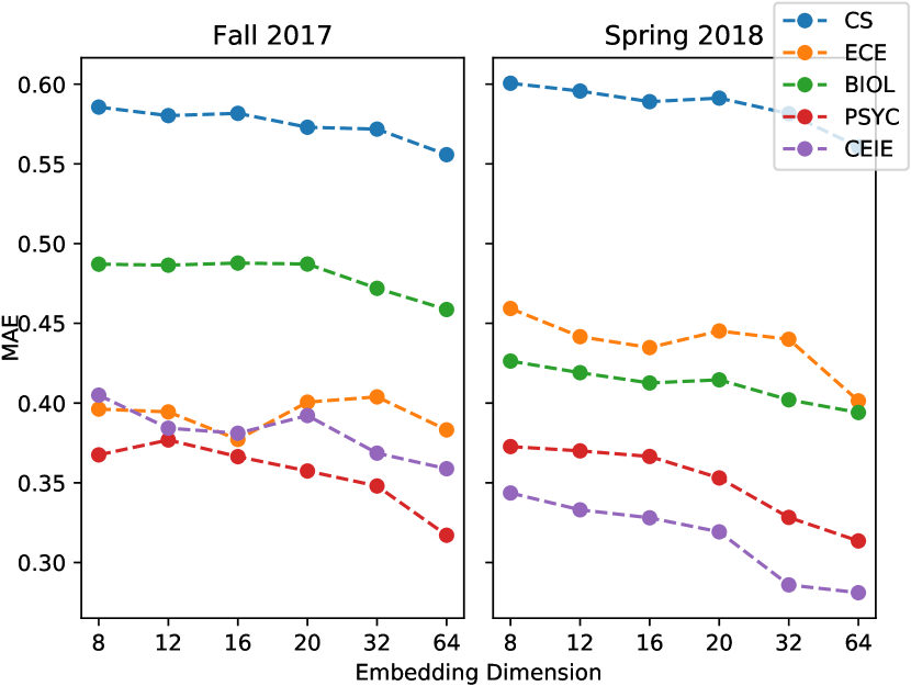
Figure 5: Sensitivity analysis on embedding dimension.

In this section, we evaluate the sensitivity of the model’s performance with respect to the dimension of the graph embedding. In Figure 5, the x-axis is the embedding dimension and y-axis is MAE for Fall 2017 and Spring 2018 datasets. From Figure 5, we can see that the model’s performance varies with the dimension size. Overall, its performance is quite stable across the different majors.

6 Conclusions

Students’ performance prediction is a fundamental task in educational data mining. Predicting students’ performance in undergraduate degree programs is a challenging task due to several reasons. First of all, undergraduate degree programs exhibit complex knowledge dependence structures. Secondly, undergraduate degree programs are flexible which means students can take courses without following specific order and they can choose to take whatever electives they are interested in. Traditional approaches like static and sequential models are not able to fully capture the complexity and flexibility of students’ data.

In this work, we proposed a novel attention-based graph convolutional networks for students’ performance prediction. The model is able to capture the relational structure underlying students’ course records data. We performed extensive experiments to evaluate the proposed model on real-world datasets. The model is evaluated in several aspects: 1) grade prediction accuracy and 2) ability to detect at-risk students. The experimental results show that our model outperformed state-of-the-art approaches in terms of both grade prediction accuracy and at-risk students detection. Finally, the attention layer provides explanations for the model’s prediction, which is essential for decision making.

7 Acknowledgements

This work was supported by the National Science Foundation grant #1447489. The computational resources was provided by ARGO, a research computing cluster provided by the Office of Research Computing at George Mason University, VA. (URL:http://orc.gmu.edu)

References

- [1] Undergraduate Retention and Graduation Rates. https://nces.ed.gov/programs/coe/indicator_ctr.asp.
- [2] M. A. Al-Barrak and M. Al-Razgan. Predicting students final gpa using decision trees: a case study. International Journal of Information and Education Technology, 6(7):528, 2016.
- [3] R. S. Baker and K. Yacef. The state of educational data mining in 2009: A review and future visions. JEDM| Journal of Educational Data Mining, 1(1):3–17, 2009.
- [4] B. Bakhshinategh, O. R. Zaiane, S. ElAtia, and D. Ipperciel. Educational data mining applications and tasks: A survey of the last 10 years. Education and Information Technologies, 23(1):537–553, 2018.
- [5] G. Balakrishnan. Predicting student retention in massive open online courses using hidden markov models. Master’s thesis, EECS Department, University of California, Berkeley, May 2013.
- [6] R. v. d. Berg, T. N. Kipf, and M. Welling. Graph convolutional matrix completion. arXiv preprint arXiv:1706.02263, 2017.
- [7] A. Elbadrawy and G. Karypis. Domain-aware grade prediction and top-n course recommendation. In Proceedings of the 10th ACM Conference on Recommender Systems, pages 183–190. ACM, 2016.
- [8] A. Elbadrawy, R. S. Studham, and G. Karypis. Collaborative multi-regression models for predicting students’ performance in course activities. In Proceedings of the Fifth International Conference on Learning Analytics And Knowledge, pages 103–107. ACM, 2015.
- [9] Q. Hu, A. Polyzou, G. Karypis, and H. Rangwala. Enriching course-specific regression models with content features for grade prediction. In 2017 IEEE International Conference on Data Science and Advanced Analytics (DSAA), pages 504–513. IEEE, 2017.
- [10] Q. Hu and H. Rangwala. Course-specific markovian models for grade prediction. In Pacific-Asia Conference on Knowledge Discovery and Data Mining, pages 29–41. Springer, 2018.
- [11] Q. Hu and H. Rangwala. Reliable deep grade prediction with uncertainty estimation. arXiv:1902.10213, 2019.
- [12] B.-H. Kim, E. Vizitei, and V. Ganapathi. Gritnet: Student performance prediction with deep learning. arXiv preprint arXiv:1804.07405, 2018.
- [13] D. P. Kingma and J. Ba. Adam: A method for stochastic optimization. arXiv preprint arXiv:1412.6980, 2014.
- [14] Y. Koren, R. Bell, and C. Volinsky. Matrix factorization techniques for recommender systems. Computer, (8):30–37, 2009.
- [15] A. Krizhevsky, I. Sutskever, and G. E. Hinton. Imagenet classification with deep convolutional neural networks. In Advances in neural information processing systems, pages 1097–1105, 2012.
- [16] C. Lang, G. Siemens, A. Wise, and D. Gasevic. Handbook of learning analytics. SOLAR, Society for Learning Analytics and Research, 2017.
- [17] Y. LeCun, Y. Bengio, et al. Convolutional networks for images, speech, and time series. The handbook of brain theory and neural networks, 3361(10):1995, 1995.
- [18] Y. LeCun, Y. Bengio, and G. Hinton. Deep learning. nature, 521(7553):436, 2015.
- [19] Y. Li, R. Yu, C. Shahabi, and Y. Liu. Diffusion convolutional recurrent neural network: Data-driven traffic forecasting. arXiv preprint arXiv:1707.01926, 2017.
- [20] S. Morsy and G. Karypis. A study on curriculum planning and its relationship with graduation gpa and time to degree. In Proceedings of the 9th International Conference on Learning Analytics & Knowledge, pages 26–35. ACM, 2019.
- [21] A. Paszke, S. Gross, S. Chintala, G. Chanan, E. Yang, Z. DeVito, Z. Lin, A. Desmaison, L. Antiga, and A. Lerer. Automatic differentiation in pytorch. In NIPS-W, 2017.
- [22] C. Piech, J. Bassen, J. Huang, S. Ganguli, M. Sahami, L. J. Guibas, and J. Sohl-Dickstein. Deep knowledge tracing. In Advances in neural information processing systems, pages 505–513, 2015.
- [23] A. Polyzou and G. Karypis. Grade prediction with models specific to students and courses. International Journal of Data Science and Analytics, 2(3-4):159–171, 2016.
- [24] C. Raffel and D. P. Ellis. Feed-forward networks with attention can solve some long-term memory problems. arXiv preprint arXiv:1512.08756, 2015.
- [25] Z. Ren, X. Ning, and H. Rangwala. Grade prediction with temporal course-wise influence. arXiv preprint arXiv:1709.05433, 2017.
- [26] C. Romero, S. Ventura, M. Pechenizkiy, and R. S. Baker. Handbook of educational data mining. CRC press, 2010.
- [27] A. M. Shahiri, W. Husain, et al. A review on predicting student’s performance using data mining techniques. Procedia Computer Science, 72:414–422, 2015.
- [28] N. Srivastava, G. Hinton, A. Krizhevsky, I. Sutskever, and R. Salakhutdinov. Dropout: a simple way to prevent neural networks from overfitting. The Journal of Machine Learning Research, 15(1):1929–1958, 2014.
- [29] V. Swamy, A. Guo, S. Lau, W. Wu, M. Wu, Z. Pardos, and D. Culler. Deep knowledge tracing for free-form student code progression. In International Conference on Artificial Intelligence in Education, pages 348–352. Springer, 2018.
- [30] M. Sweeney, H. Rangwala, J. Lester, and A. Johri. Next-term student performance prediction: A recommender systems approach. arXiv preprint arXiv:1604.01840, 2016.
- [31] S. Umair and M. M. Sharif. Predicting students grades using artificial neural networks and support vector machine. In Encyclopedia of Information Science and Technology, Fourth Edition, pages 5169–5182. IGI Global, 2018.
- [32] R. Wang, G. Harari, P. Hao, X. Zhou, and A. T. Campbell. Smartgpa: how smartphones can assess and predict academic performance of college students. In Proceedings of the 2015 ACM international joint conference on pervasive and ubiquitous computing, pages 295–306. ACM, 2015.
- [33] Y. Wang, Y. Sun, Z. Liu, S. E. Sarma, M. M. Bronstein, and J. M. Solomon. Dynamic graph cnn for learning on point clouds. arXiv preprint arXiv:1801.07829, 2018.
- [34] S. Yan, Y. Xiong, and D. Lin. Spatial temporal graph convolutional networks for skeleton-based action recognition. In Thirty-Second AAAI Conference on Artificial Intelligence, 2018.
- [35] M. V. Yudelson, K. R. Koedinger, and G. J. Gordon. Individualized bayesian knowledge tracing models. In International conference on artificial intelligence in education, pages 171–180. Springer, 2013.