Resilient Primal-Dual Optimization Algorithms for Distributed Resource Allocation

Berkay Turan   César A. Uribe   Hoi-To Wai    Mahnoosh Alizadeh
Abstract

Distributed algorithms for multi-agent resource allocation can provide privacy and scalability over centralized algorithms in many cyber-physical systems. However, the distributed nature of these algorithms can render these systems vulnerable to man-in-the-middle attacks that can lead to non-convergence and infeasibility of resource allocation schemes. In this paper, we propose attack-resilient distributed algorithms based on primal-dual optimization when Byzantine attackers are present in the system. In particular, we design attack-resilient primal-dual algorithms for static and dynamic impersonation attacks by means of robust statistics. For static impersonation attacks, we formulate a robustified optimization model and show that our algorithm guarantees convergence to a neighborhood of the optimal solution of the robustified problem. On the other hand, a robust optimization model is not required for the dynamic impersonation attack scenario and we are able to design an algorithm that is shown to converge to a near-optimal solution of the original problem. We analyze the performances of our algorithms through both theoretical and computational studies.

footnotetext: Authors have equal contribution. B. Turan and M. Alizadeh are with Dept. of ECE, UCSB, Santa Barbara, CA, USA. C. A. Uribe is with LIDS, MIT, Cambridge, MA, USA. H. T. Wai is with Dept. of SEEM, CUHK, Shatin, Hong Kong. This work is partially supported by UCOP Grant LFR-18-548175, NSF grant #1847096, CUHK Direct Grant #4055113, and the Yahoo! Research Faculty Engagement Program. E-mails: bturan@ucsb.edu, cauribe@mit.edu, htwai@se.cuhk.edu.hk, alizadeh@ucsb.edu

I Introduction

A number of multi-agent optimization problems arise in a wide range of resource allocation systems that fall under the general umbrella of Network Utility Maximization problems: in the pioneering example of congestion control in data networks [1, 2]; in determining the optimal price of electricity and enabling more efficient demand supply balancing in smart power distribution systems [3, 4]; in managing user transmit powers and data rates in wireless cellular networks [5]; in determining optimal caching policies by content delivery networks [6]; in optimizing power consumption in wireless sensor networks with energy-restricted batteries [7, 8]; and in designing congestion control systems in urban traffic networks [9]. The shared goal among the above-mentioned problems is to minimize the sum of N𝑁N user-specific cost functions, subject to a set of coupling constraints that depend on users’ decisions.

In these resource allocation problems, the user-specific cost functions and the set of coupling constraints are considered private information to the users and to a central coordinator, respectively. Consequently, it is necessary to solve these problems in a distributed fashion allowing the agents to cooperate through communication with a central coordinator. Among others, primal-dual optimization methods [10] have been advocated as they naturally give rise to decomposable algorithms that favor distributed implementation [11]. In addition to their practical success, these methods are supported by strong theoretical guarantees where fast convergence to a near-optimal solution is well established [10].

However, the distributed nature of these methods also exposes the system to vulnerabilities not faced by their traditional centralized counterpart. Many of the existing algorithms assume the agents, and the communication channels between the central coordinator and the agents, to be completely trustworthy. In this paper, we consider the setting where these communications are susceptible to adversarial attacks. An attacker can take over network sub-systems, and deliberately edit the messages communicated to the central coordinator to any arbitrary value, i.e., a Byzantine attack. As we will demonstrate, this might result in an unstable system with possible damages to hardware and the system overall.

Our goal is to design attack-resilient primal-dual algorithms in order to solve multi-agent resource allocation problems in presence of Byzantine attackers. If a communication channel is attacked and becomes compromised, the attacker can modify messages and/or inject fresh messages into the network on the agents’ behalf. We consider two scenarios with different attacker capabilities. A static impersonation attack scenario considers the set of agents communicating through compromised channels to be the same for the duration of the algorithm, whereas a dynamic impersonation attack scenario considers the case where all agents are susceptible to attacks and hence communicate through compromised channels for a limited fraction of the algorithm’s runtime. Our main contributions are as follows:

  • We propose resilient distributed resource allocation algorithms under the two aforementioned attack scenarios that rely on robust mean estimation.

  • We provide convergence guarantees of the proposed algorithms. We show that our algorithm for the dynamic impersonation attack scenario converges to the optimal solution of the regularized problem, while our algorithm for the static impersonation attack scenario converges to an 𝒪(α12)𝒪superscriptsubscript𝛼12\mathcal{O}(\alpha_{1}^{2}) neighborhood of the optimal solution of a robustified and regularized optimization model, where α1[0,12)subscript𝛼1012\alpha_{1}\in[0,\frac{1}{2}) is a known upper bound on fraction of attacked channels.

  • We provide empirical evidence that supports our theoretical results on convergence and preventing constraint violation. We do so via computational simulations on electric vehicle charging and power distribution applications.

Related work: Vulnerabilities of various types of distributed algorithms have been identified and addressed in a number of recent studies. Relevant examples can be found in [12, 13, 14, 15, 16, 17, 18, 19, 20] which study secure decentralized algorithms on a general network topology but consider consensus-based optimization models. There are two fundamental differences between distributed resource allocation and consensus problems that make these algorithms inapplicable in our case:

  • In resource allocation problems, each agent is solving for their own optimal level of resource consumption, i.e., each agent is solving for their own parameter, whereas consensus problems focus on all agents solving for a shared (global) parameter.

  • Unlike resilient consensus algorithms, in resource allocation problems pertaining to access to critical infrastructure systems such as power or transportation networks, one cannot simply block a set of users’ access to the network even if they are deemed likely to be attackers.

A recently popular line of works in [21, 22, 23, 24, 25] focuses on building resilient algorithms for distributed statistical learning. A crucial difference from this work is that they assume identical functions across the agents. In fact, we employ robust statistics [26, 27] to develop our resilient algorithms, and particularly, we develop novel results for robust mean estimation, a topic that is recently rekindled in [28, 29, 30].

The present paper is a revised and extended version of the preliminary conference report [31]. This paper expands [31] into multiple attack scenarios and includes numerical studies.

Paper Organization: The remainder of the paper is organized as follows. In Section II, we provide an overview of the basic primal-dual algorithm for resource allocation. In Section III, we formally define two Byzantine attack models and demonstrate how Byzantine attacks can alter the primal-dual optimization procedure. In Section IV, we present two attack-resilient primal-dual algorithms corresponding to the different attack scenarios along with their convergence analysis. In Section V, we provide numerical results for our algorithms.

Notations. Unless otherwise specified, \|\cdot\| denotes the standard Euclidean norm. For any N𝑁N\in\mathbb{N}, [N]delimited-[]𝑁[N] denotes the finite set {1,,N}1𝑁\{1,...,N\}. Given 𝜽𝜽\bm{\theta}, 𝜽isubscript𝜽𝑖\bm{\theta}_{i} indicates the i𝑖i’th block/entry of 𝜽𝜽\bm{\theta} that corresponds to the parameter of agent i𝑖i. 𝜽i,jsubscript𝜽𝑖𝑗\bm{\theta}_{i,j} denotes the j𝑗j’th element of vector 𝜽isubscript𝜽𝑖\bm{\theta}_{i}.

II Overview of Primal-Dual Algorithm for Resource Allocation

1:  for k=1,2,𝑘12k=1,2,... do
2:      (Communication stage):
  1. (a)

    Central coordinator receives {𝜽i(k)}i=1Nsuperscriptsubscriptsuperscriptsubscript𝜽𝑖𝑘𝑖1𝑁\{\bm{\theta}_{i}^{(k)}\}_{i=1}^{N} from agents and computes 𝜽¯(k):=1Ni=1N𝜽i(k)assignsuperscript¯𝜽𝑘1𝑁superscriptsubscript𝑖1𝑁superscriptsubscript𝜽𝑖𝑘\textstyle{\overline{\bm{\theta}}^{(k)}\vcentcolon=\frac{1}{N}\sum_{i=1}^{N}\bm{\theta}_{i}^{(k)}}, {𝜽gt(𝜽¯(k))}t=1Tsuperscriptsubscriptsubscript𝜽subscript𝑔𝑡superscript¯𝜽𝑘𝑡1𝑇\{\nabla_{\bm{\theta}}g_{t}(\overline{\bm{\theta}}^{(k)})\}_{t=1}^{T}.

  2. (b)

    Central coordinator broadcasts the vector 𝒈¯(k):=t=1Tλt(k)𝜽gt(𝜽¯(k))assignsuperscript¯𝒈𝑘superscriptsubscript𝑡1𝑇superscriptsubscript𝜆𝑡𝑘subscript𝜽subscript𝑔𝑡superscript¯𝜽𝑘\overline{\bm{g}}^{(k)}\vcentcolon=\sum_{t=1}^{T}\lambda_{t}^{(k)}\nabla_{\bm{\theta}}g_{t}(\overline{\bm{\theta}}^{(k)}) to agents.

3:      (Computation stage):
  1. (a)

    Agent i𝑖i computes the update for 𝜽i(k+1)superscriptsubscript𝜽𝑖𝑘1\bm{\theta}_{i}^{(k+1)} according to (4a) using the received 𝒈¯(k)superscript¯𝒈𝑘\overline{\bm{g}}^{(k)}.

  2. (b)

    The central coordinator computes the update for 𝝀(k+1)superscript𝝀𝑘1\bm{\lambda}^{(k+1)} according to (4b).

4:  end for
Algorithm 1 PD-DRA Procedure.

We consider the following multi-agent optimization problem with an objective to minimize the average cost incurred by the agents, subject to a set of constraints that are functions of the average of the agents’ parameters:

min𝜽id,isubscript𝜽𝑖superscript𝑑for-all𝑖\displaystyle\underset{\bm{\theta}_{i}\in\mathbb{R}^{d},\forall i}{\min} f(𝜽):=1Ni=1Nfi(𝜽i)assign𝑓𝜽1𝑁superscriptsubscript𝑖1𝑁subscript𝑓𝑖subscript𝜽𝑖\displaystyle{\color[rgb]{0,0,0}f}(\bm{\theta})\vcentcolon=\frac{1}{N}\sum_{i=1}^{N}{\color[rgb]{0,0,0}f_{i}}(\bm{\theta}_{i}) (1)
subject to gt(1Ni=1N𝜽i)0,subscript𝑔𝑡1𝑁superscriptsubscript𝑖1𝑁subscript𝜽𝑖0\displaystyle g_{t}\left({\textstyle\frac{1}{N}\sum_{i=1}^{N}\bm{\theta}_{i}}\right)\leq 0, t=1,,T,𝑡1𝑇\displaystyle t=1,\dots,T,
𝜽i𝒞i,subscript𝜽𝑖subscript𝒞𝑖\displaystyle\bm{\theta}_{i}\in\mathcal{C}_{i}, i=1,,N,𝑖1𝑁\displaystyle i=1,\dots,N,

where fi():d:subscript𝑓𝑖superscript𝑑{\color[rgb]{0,0,0}f_{i}}(\cdot):\mathbb{R}^{d}\rightarrow\mathbb{R} is the continuously differentiable and convex cost function of agent i𝑖i and gt():d:subscript𝑔𝑡superscript𝑑g_{t}(\cdot):\mathbb{R}^{d}\rightarrow\mathbb{R} are continuously differentiable and convex set of constraints. The parameter 𝜽isubscript𝜽𝑖\bm{\theta}_{i} of agent i𝑖i is constrained to be in a compact convex set 𝒞idsubscript𝒞𝑖superscript𝑑\mathcal{C}_{i}\in\mathbb{R}^{d}.

Running Example (Resource Allocation Problem).

Throughout the paper, we use the following toy example as a running example to clarify the concepts and the methods: We consider an EV charging example with 5 agents. The cost function fi()subscript𝑓𝑖f_{i}(\cdot) is monotone decreasing and is the same for all agents. As an example, we set fi(𝛉i)=(𝛉i10)2subscript𝑓𝑖subscript𝛉𝑖superscriptsubscript𝛉𝑖102f_{i}(\bm{\theta}_{i})=(\bm{\theta}_{i}-10)^{2} as the quadratic cost function which is monotonically decreasing for 0𝛉i100subscript𝛉𝑖100\leq\bm{\theta}_{i}\leq 10. There is a charging station with 5 EV charging points, three of which have a maximum charging rate of 777kW, and two have a rate of 101010kW. The total rate at which the charging station is able to deliver electricity is determined by the grid, and let it be upper bounded by 252525kW (hence, the average rate is upper bounded by 255=52555\frac{25}{5}=5kW). Accordingly, the constraints of this system are stated as:

g((1/5)i=15𝜽i):=(1/5)i=15𝜽i50,assign𝑔15superscriptsubscript𝑖15subscript𝜽𝑖15superscriptsubscript𝑖15subscript𝜽𝑖50\displaystyle\textstyle g\big{(}(1/5)\sum_{i=1}^{5}\bm{\theta}_{i}\big{)}\vcentcolon=(1/5)\sum_{i=1}^{5}\bm{\theta}_{i}-5\leq 0,
0𝜽i7,i=1,2,3,formulae-sequence0subscript𝜽𝑖7𝑖123\displaystyle 0\leq\bm{\theta}_{i}\leq 7,\quad i=1,2,3,
0𝜽i10,i=4,5.formulae-sequence0subscript𝜽𝑖10𝑖45\displaystyle 0\leq\bm{\theta}_{i}\leq 10,\quad i=4,5.

Note that 𝛉𝛉\bm{\theta} is a real number, hence dimension d=1𝑑1d=1. The optimal solution in this example is to deliver electricity at a rate of 555kW to all agents due to symmetry.

The optimization problem in (1) can not be solved centrally, because the utility functions fi()subscript𝑓𝑖{\color[rgb]{0,0,0}f_{i}}(\cdot) are private to the agents, and furthermore the coupling constraints on the resources are only known by a central coordinator. Accordingly, the goal of the primal-dual distributed resource allocation (PD-DRA) procedure in Algorithm 1 is to solve (1) in a distributed manner, where the agents observe a pricing signal received from the central coordinator and communicate their parameters to the central coordinator [10]. Consequent to this information exchange, the pricing signal and the agents’ parameters are updated by the central coordinator and by the individual agents, respectively.

In order to derive the update rules used by Algorithm 1, we first consider the Lagrangian function of (1):

({𝜽i}i=1N;𝝀):=1Ni=1Nfi(𝜽i)+t=1Tλtgt(1Ni=1N𝜽i),assignsuperscriptsubscriptsubscript𝜽𝑖𝑖1𝑁𝝀1𝑁superscriptsubscript𝑖1𝑁subscript𝑓𝑖subscript𝜽𝑖superscriptsubscript𝑡1𝑇subscript𝜆𝑡subscript𝑔𝑡1𝑁superscriptsubscript𝑖1𝑁subscript𝜽𝑖{\cal L}(\{\bm{\theta}_{i}\}_{i=1}^{N};\bm{\lambda})\vcentcolon=\frac{1}{N}\sum_{i=1}^{N}{\color[rgb]{0,0,0}f_{i}}(\bm{\theta}_{i})+\sum_{t=1}^{T}\lambda_{t}\!~{}g_{t}\Big{(}\frac{1}{N}\sum_{i=1}^{N}\bm{\theta}_{i}\Big{)}, (2)

where λt0subscript𝜆𝑡0\lambda_{t}\geq 0 is the dual variable associated with constraint gt()subscript𝑔𝑡g_{t}(\cdot) and 𝝀=[λ1λT]+T𝝀superscriptdelimited-[]subscript𝜆1subscript𝜆𝑇superscriptsubscript𝑇\bm{\lambda}=[\lambda_{1}\dots\lambda_{T}]^{\intercal}\in\mathbb{R}_{+}^{T} is the vector of the dual variables. Under strong duality (e.g., when the Slater’s condition holds), solving problem (1) is equivalent to solving its dual problem:

max𝝀+Tmin𝜽i𝒞i,i({𝜽i}i=1N;𝝀).subscript𝝀superscriptsubscript𝑇subscriptsubscript𝜽𝑖subscript𝒞𝑖for-all𝑖superscriptsubscriptsubscript𝜽𝑖𝑖1𝑁𝝀\max_{\bm{\lambda}\in\mathbb{R}_{+}^{T}}~{}\min_{\bm{\theta}_{i}\in\mathcal{C}_{i},\forall i}~{}{\cal L}(\{\bm{\theta}_{i}\}_{i=1}^{N};\bm{\lambda}). (P)

As suggested in [10], we consider a regularized version of (P). Let us define

υ({𝜽i}i=1N;𝝀):=({𝜽i}i=1N;𝝀)+υ2Ni=1N𝜽i2υ2𝝀2,assignsubscript𝜐superscriptsubscriptsubscript𝜽𝑖𝑖1𝑁𝝀superscriptsubscriptsubscript𝜽𝑖𝑖1𝑁𝝀𝜐2𝑁superscriptsubscript𝑖1𝑁superscriptdelimited-∥∥subscript𝜽𝑖2𝜐2superscriptdelimited-∥∥𝝀2\begin{split}&{\cal L}_{\upsilon}(\{\bm{\theta}_{i}\}_{i=1}^{N};\bm{\lambda})\vcentcolon=\\ &\textstyle{\cal L}(\{\bm{\theta}_{i}\}_{i=1}^{N};\bm{\lambda})+\frac{\upsilon}{2N}\sum_{i=1}^{N}\|\bm{\theta}_{i}\|^{2}-\frac{\upsilon}{2}\|\bm{\lambda}\|^{2},\end{split} (3)

such that υ()subscript𝜐{\cal L}_{\upsilon}(\cdot) is υ𝜐\upsilon-strongly convex and υ𝜐\upsilon-strongly concave in {𝜽i}i=1Nsuperscriptsubscriptsubscript𝜽𝑖𝑖1𝑁\{\bm{\theta}_{i}\}_{i=1}^{N} and 𝝀𝝀\bm{\lambda}, respectively.

Remark 1.

Adding regularization terms is a typical technique used in optimization, called dual smoothing[32]. We add the regularization terms for the purposes of convergence analysis used in this paper, which can be applied on strongly convex/concave functions. Indeed adding the regularization terms might change the solution of the original optimization problem. However, as explained in [33, Proposition 5.2], by an appropriate selection of the regularization parameters, we can recover an optimality gap guarantee for the original problem based on the solution to the regularized problem.

We define the regularized problem as:

max𝝀+Tmin𝜽i𝒞i,iυ({𝜽i}i=1N;𝝀).subscript𝝀superscriptsubscript𝑇subscriptsubscript𝜽𝑖subscript𝒞𝑖for-all𝑖subscript𝜐superscriptsubscriptsubscript𝜽𝑖𝑖1𝑁𝝀\max_{\bm{\lambda}\in\mathbb{R}_{+}^{T}}~{}\min_{\bm{\theta}_{i}\in\mathcal{C}_{i},\forall i}~{}{\cal L_{\upsilon}}(\{\bm{\theta}_{i}\}_{i=1}^{N};\bm{\lambda}). (Pυ)

Let γ>0𝛾0\gamma>0 be the step size and k+𝑘subscriptk\in\mathbb{Z}_{+} be the iteration index. The primal-dual recursion performs projected gradient descent/ascent on the primal/dual variables as follows:

𝜽i(k+1)=superscriptsubscript𝜽𝑖𝑘1absent\displaystyle\bm{\theta}_{i}^{(k+1)}= (4a)
𝒫𝒞i(𝜽i(k)γ𝜽iυ({𝜽i(k)}i=1N;𝝀(k))),i[N],subscript𝒫subscript𝒞𝑖superscriptsubscript𝜽𝑖𝑘𝛾subscriptsubscript𝜽𝑖subscript𝜐superscriptsubscriptsuperscriptsubscript𝜽𝑖𝑘𝑖1𝑁superscript𝝀𝑘for-all𝑖delimited-[]𝑁\displaystyle~{}~{}~{}~{}~{}~{}{\cal P}_{\mathcal{C}_{i}}\big{(}\bm{\theta}_{i}^{(k)}-\gamma\!~{}\nabla_{\bm{\theta}_{i}}{\cal L}_{\upsilon}(\{\bm{\theta}_{i}^{(k)}\}_{i=1}^{N};\bm{\lambda}^{(k)})\big{)},\;\forall i\in[N],
𝝀(k+1)=[𝝀(k)+γ𝝀υ({𝜽i(k)}i=1N;𝝀(k))]+,superscript𝝀𝑘1subscriptdelimited-[]superscript𝝀𝑘𝛾subscript𝝀subscript𝜐superscriptsubscriptsuperscriptsubscript𝜽𝑖𝑘𝑖1𝑁superscript𝝀𝑘\displaystyle\bm{\lambda}^{(k+1)}=\big{[}\bm{\lambda}^{(k)}+\gamma\!~{}\nabla_{\bm{\lambda}}{\cal L}_{\upsilon}(\{\bm{\theta}_{i}^{(k)}\}_{i=1}^{N};\bm{\lambda}^{(k)})\big{]}_{+}, (4b)

where 𝒫𝒞i()subscript𝒫subscript𝒞𝑖{\cal P}_{\mathcal{C}_{i}}(\cdot) is the Euclidean projection operator to set 𝒞isubscript𝒞𝑖\mathcal{C}_{i} and []+subscriptdelimited-[][\cdot]_{+} denotes max{,0}0\max\{\cdot,0\} operator. According to (3), the gradients with respect to (w.r.t.) the primal and the dual variables are given respectively by:

𝜽iυ({𝜽i(k)}i=1N;𝝀(k))=1N(𝜽ifi(𝜽i(k))+υ𝜽i(k)+t=1Tλt(k)𝜽gt(𝜽)|𝜽=1Ni=1N𝜽i(k)),subscriptsubscript𝜽𝑖subscript𝜐superscriptsubscriptsuperscriptsubscript𝜽𝑖𝑘𝑖1𝑁superscript𝝀𝑘1𝑁subscriptsubscript𝜽𝑖subscript𝑓𝑖superscriptsubscript𝜽𝑖𝑘𝜐superscriptsubscript𝜽𝑖𝑘evaluated-atsuperscriptsubscript𝑡1𝑇superscriptsubscript𝜆𝑡𝑘subscript𝜽subscript𝑔𝑡𝜽𝜽1𝑁superscriptsubscript𝑖1𝑁superscriptsubscript𝜽𝑖𝑘\begin{split}&\nabla_{\bm{\theta}_{i}}{\cal L}_{\upsilon}(\{\bm{\theta}_{i}^{(k)}\}_{i=1}^{N};\bm{\lambda}^{(k)})=\frac{1}{N}\Big{(}\nabla_{\bm{\theta}_{i}}{\color[rgb]{0,0,0}f_{i}}(\bm{\theta}_{i}^{(k)})+\upsilon\!~{}\bm{\theta}_{i}^{(k)}\\ &\hskip 45.52458pt\textstyle+\sum_{t=1}^{T}\lambda_{t}^{(k)}\nabla_{\bm{\theta}}g_{t}(\bm{\theta})\Big{|}_{\bm{\theta}=\frac{1}{N}\sum_{i=1}^{N}\bm{\theta}_{i}^{(k)}}\Big{)},\\ \end{split} (5a)
[𝝀υ({𝜽i(k)}i=1N;𝝀(k))]t=gt(1Ni=1N𝜽i(k))υλt(k),subscriptdelimited-[]subscript𝝀subscript𝜐superscriptsubscriptsuperscriptsubscript𝜽𝑖𝑘𝑖1𝑁superscript𝝀𝑘𝑡subscript𝑔𝑡1𝑁superscriptsubscript𝑖1𝑁superscriptsubscript𝜽𝑖𝑘𝜐superscriptsubscript𝜆𝑡𝑘\begin{split}&\big{[}\nabla_{\bm{\lambda}}{\cal L}_{\upsilon}(\{\bm{\theta}_{i}^{(k)}\}_{i=1}^{N};\bm{\lambda}^{(k)})\big{]}_{t}=g_{t}\Big{(}{\textstyle\frac{1}{N}\sum_{i=1}^{N}}\bm{\theta}_{i}^{(k)}\Big{)}-\upsilon\!~{}\lambda_{t}^{(k)},\end{split} (5b)

for all i𝑖i, t𝑡t. It is worthwhile to highlight that both gradients depend on the average parameter 𝜽¯(k):=1Ni=1N𝜽i(k)assignsuperscript¯𝜽𝑘1𝑁superscriptsubscript𝑖1𝑁superscriptsubscript𝜽𝑖𝑘\overline{\bm{\theta}}^{(k)}\vcentcolon=\frac{1}{N}\sum_{i=1}^{N}\bm{\theta}_{i}^{(k)}. From the above equations (5a) and (5b), we can determine which variables should be communicated between the central coordinator and the agents so that the gradients can be computed locally, see Algorithm 1.

Refer to caption
(a) A static impersonation attack scenario, agents 4 and 5 are permanently communicating through compromised channels.
Refer to caption
(b) A dynamic impersonation scenario, where the set of agents communicating through compromised channels are changing.
Figure 1: Illustration of (a) static impersonation attack, and (b) dynamic impersonation attack. Blue arrows represent trustworthy channels, whereas red arrows represent compromised channels.

Since the regularized primal-dual problem is strongly convex/concave in primal/dual variables, Algorithm 1 converges linearly to the optimal solution of (Pυ) [10]. To study this, let us concatenate the primal and the dual variables and denote 𝒛(k):=({𝜽i(k)}i=1N,𝝀(k))assignsuperscript𝒛𝑘superscriptsubscriptsuperscriptsubscript𝜽𝑖𝑘𝑖1𝑁superscript𝝀𝑘{\bm{z}}^{(k)}\vcentcolon=(\{\bm{\theta}_{i}^{(k)}\}_{i=1}^{N},\bm{\lambda}^{(k)}) as the primal-dual variable at the k𝑘kth iteration and define the mapping 𝚽(𝒛(k))𝚽superscript𝒛𝑘\bm{\Phi}({\bm{z}}^{(k)}) as:

𝚽(𝒛(k)):=(𝜽υ({𝜽i(k)}i=1N,𝝀(k))𝝀υ({𝜽i(k)}i=1N,𝝀(k))).assign𝚽superscript𝒛𝑘subscript𝜽subscript𝜐superscriptsubscriptsuperscriptsubscript𝜽𝑖𝑘𝑖1𝑁superscript𝝀𝑘subscript𝝀subscript𝜐superscriptsubscriptsuperscriptsubscript𝜽𝑖𝑘𝑖1𝑁superscript𝝀𝑘\bm{\Phi}({\bm{z}}^{(k)})\vcentcolon=\left(\begin{array}[]{c}\nabla_{\bm{\theta}}{\cal L}_{\upsilon}(\{\bm{\theta}_{i}^{(k)}\}_{i=1}^{N},\bm{\lambda}^{(k)})\\ -\nabla_{\bm{\lambda}}{\cal L}_{\upsilon}(\{\bm{\theta}_{i}^{(k)}\}_{i=1}^{N},\bm{\lambda}^{(k)})\end{array}\right). (6)
Proposition 1.

[10, Theorem 3.5] Assume that the map 𝚽(𝐳(k))𝚽superscript𝐳𝑘\bm{\Phi}({\bm{z}}^{(k)}) is LΦsubscript𝐿ΦL_{\Phi} Lipschitz continuous. For all k1𝑘1k\geq 1, we have

𝒛(k+1)𝒛2(12γυ+γ2LΦ2)𝒛(k)𝒛2,superscriptnormsuperscript𝒛𝑘1superscript𝒛212𝛾𝜐superscript𝛾2superscriptsubscript𝐿Φ2superscriptnormsuperscript𝒛𝑘superscript𝒛2\|{\bm{z}}^{(k+1)}-{\bm{z}}^{\star}\|^{2}\leq(1-2\gamma\upsilon+\gamma^{2}L_{\Phi}^{2})\!~{}\|{\bm{z}}^{(k)}-{\bm{z}}^{\star}\|^{2}, (7)

where 𝐳superscript𝐳{\bm{z}}^{\star} is a saddle point to the (Pυ). Setting γ=υ/LΦ2𝛾𝜐superscriptsubscript𝐿Φ2\gamma=\upsilon/L_{\Phi}^{2} gives 𝐳(k+1)𝐳2(1υ2/LΦ2)𝐳(k)𝐳2superscriptnormsuperscript𝐳𝑘1superscript𝐳21superscript𝜐2superscriptsubscript𝐿Φ2superscriptnormsuperscript𝐳𝑘superscript𝐳2\|{\bm{z}}^{(k+1)}-{\bm{z}}^{\star}\|^{2}\leq\big{(}1-\upsilon^{2}/L_{\Phi}^{2}\big{)}\|{\bm{z}}^{(k)}-{\bm{z}}^{\star}\|^{2}, k1for-all𝑘1\forall~{}k\geq 1.

III Problem Formulation

Even though the PD-DRA provides strong theoretical convergence guarantee, it relies on error-free communication between the central coordinator and the agents, and is not robust to attacks on the channels between the agents and the central coordinator, as described below.

We study a situation when the uplink communication channels between some of the agents and the central coordinator are compromised.111This paper studies the case where only uplink channels are compromised. However, the case of downlink corruption can also be addressed. Since the downlink channel is a broadcast channel, a compromised downlink channel results in no agent receiving a trustworthy pricing signal. In that case, there is no optimization method based solution to that problem since there is no communication. If we assume however that all the downlink channels are point-to-point between the central coordinator and each agent, the methods developed in this paper can be applied in a similar fashion. Let 𝒜(k)[N]superscript𝒜𝑘delimited-[]𝑁\mathcal{A}^{(k)}\subset[N] be the set of agents communicating through compromised uplink channels at iteration k𝑘k, whose identities are unknown to the central coordinator, and let (k):=[N]𝒜(k)assignsuperscript𝑘delimited-[]𝑁superscript𝒜𝑘\mathcal{H}^{(k)}\vcentcolon=[N]\setminus{\cal A}^{(k)} be the set of agents communicating through trustworthy uplink channels at iteration k𝑘k. Instead of receiving 𝜽i(k)superscriptsubscript𝜽𝑖𝑘\bm{\theta}_{i}^{(k)} from each agent i[N]𝑖delimited-[]𝑁i\in[N] at iteration k𝑘k (Algorithm 1 Step 2(a)), the central coordinator receives the following messages:

𝒓i(k)={𝜽i(k),ifi(k),𝒃i(k),ifi𝒜(k).superscriptsubscript𝒓𝑖𝑘casessuperscriptsubscript𝜽𝑖𝑘if𝑖superscript𝑘superscriptsubscript𝒃𝑖𝑘if𝑖superscript𝒜𝑘{\bm{r}}_{i}^{(k)}=\begin{cases}\bm{\theta}_{i}^{(k)},&\text{if}~{}i\in\mathcal{H}^{(k)},\\ {\bm{b}}_{i}^{(k)},&\text{if}~{}i\in\mathcal{A}^{(k)}.\end{cases} (8)

We consider a Byzantine attack scenario, under which the messages sent through the compromised channels, 𝒃i(k)superscriptsubscript𝒃𝑖𝑘\bm{b}_{i}^{(k)}, can be chosen arbitrarily by an adversary. This also encompasses faulty messages due to erroneous inputs or erroneous channels, since we set no restrictions on 𝒃i(k)superscriptsubscript𝒃𝑖𝑘\bm{b}_{i}^{(k)}. The adversary’s goal is to harm the system and cause suboptimalities. When the messages are erroneous or chosen adversarily, the central coordinator computes the gradients and therefore the pricing signal using these erroneous messages. The agents then update their parameters based on this erroneous pricing signal, which can lead to an overall suboptimal resource allocation. Moreover, the choice of the compromised channels 𝒜(k)superscript𝒜𝑘{\cal A}^{(k)} affects the impact of the attack and the precautions to be taken in order to defend against the attack. As such, we study two Byzantine attack scenarios that differ in the set of the compromised channels as illustrated in Figure 1.

Running Example (Byzantine Attack).

Let agent 1 be communicating through a compromised channel at all iterations, i.e., 𝒜(k)={1}superscript𝒜𝑘1{\cal A}^{(k)}=\{1\}, kfor-all𝑘\forall k. The compromised message sent to the central coordinator is 𝐛1(k)=1subscriptsuperscript𝐛𝑘11{\bm{b}}^{(k)}_{1}=1kW, kfor-all𝑘\forall k. This means that irrespective of 𝛉1(k)superscriptsubscript𝛉1𝑘\bm{\theta}_{1}^{(k)}, the central coordinator receives a message indicating agent 1 is willing to charge at rate of 111kW.

III-A Attack scenarios

  1. 1.

    A static impersonation attack, where an adversary takes over a subset of uplink channels permanently and the set of agents communicating through compromised channels is fixed (i.e., 𝒜(k)=𝒜,ksuperscript𝒜𝑘𝒜for-all𝑘\mathcal{A}^{(k)}=\mathcal{A},~{}\forall k). Consequently, the central coordinator is never able to communicate reliably with agents i𝒜𝑖𝒜i\in\mathcal{A}. In this case, it is not feasible to optimize the original problem (P) since the contribution from f(𝜽i):i𝒜:𝑓subscript𝜽𝑖𝑖𝒜f(\bm{\theta}_{i}):i\in{\cal A} becomes unknown to the central coordinator. Yet, we assume that it is also not possible to deny access to resources to agents who are suspected of potentially being under attack. As a compromise, we formulate the following optimization problem:

    min𝜽i𝒞i,iformulae-sequencesubscript𝜽𝑖subscript𝒞𝑖𝑖\displaystyle\underset{\bm{\theta}_{i}\in\mathbb{\mathcal{C}}_{i},i\in\cal{H}}{\min} f(𝜽):=1Nifi(𝜽i)assign𝑓𝜽1𝑁subscript𝑖subscript𝑓𝑖subscript𝜽𝑖\displaystyle{\color[rgb]{0,0,0}f}(\bm{\theta})\vcentcolon=\frac{1}{N}\sum_{i\in\cal{H}}{\color[rgb]{0,0,0}f_{i}}(\bm{\theta}_{i}) (9)
    subject to max𝜽j𝒞j,j𝒜gt(1Ni=1N𝜽i)0,formulae-sequencesubscript𝜽𝑗subscript𝒞𝑗𝑗𝒜subscript𝑔𝑡1𝑁superscriptsubscript𝑖1𝑁subscript𝜽𝑖0\displaystyle\underset{\bm{\theta}_{j}\in\mathcal{C}_{j},j\in\mathcal{A}}{\max}g_{t}\left({\textstyle\frac{1}{N}\sum_{i=1}^{N}\bm{\theta}_{i}}\right)\leq 0, t[T].for-all𝑡delimited-[]𝑇\displaystyle\forall t\in[T].

    The objective of (9) is to minimize the cost of the agents with trustworthy channels subject to a robust set of constraints that consider the worst case scenario, in which the parameters of the agents with compromised channels are assumed to be maximizing the constraints (e.g., those agents are assumed to be consuming the maximum amount of resources). It is critical to mention that during a primal-dual algorithm scheme, the messages received through the compromised channels can be anything. The robust approach is to however ignore those messages, and assume that the parameters of the agents communicating through those channels are maximizing the constraints so that the operation of the system is feasible under any circumstance. Our goal is to develop an attack-resilient PD-DRA to solve the robust optimization problem (9).

    Running Example (Robust Optimization Model).

    Since agent 1 is sending a compromised message of 111kW and their true parameter can be anything, the worst-case approach is to assume that they are charging at the maximum rate, which is 777kW for that agent. Hence, the robust constraint is:

    max𝜽j𝒞j,j𝒜g(15i=15𝜽i)=max𝜽j𝒞j,j𝒜15i=15𝜽i5=15i𝜽i+max𝜽j𝒞j,j𝒜15j𝒜𝜽j5=45𝜽¯3.6,formulae-sequencesubscript𝜽𝑗subscript𝒞𝑗𝑗𝒜𝑔15superscriptsubscript𝑖15subscript𝜽𝑖formulae-sequencesubscript𝜽𝑗subscript𝒞𝑗𝑗𝒜15superscriptsubscript𝑖15subscript𝜽𝑖515subscript𝑖subscript𝜽𝑖formulae-sequencesubscript𝜽𝑗subscript𝒞𝑗𝑗𝒜15subscript𝑗𝒜subscript𝜽𝑗545subscript¯𝜽3.6\begin{split}&\underset{\bm{\theta}_{j}\in\mathcal{C}_{j},j\in\mathcal{A}}{\max}g\left({\frac{1}{5}\sum_{i=1}^{5}\bm{\theta}_{i}}\right)=\underset{\bm{\theta}_{j}\in\mathcal{C}_{j},j\in\mathcal{A}}{\max}\frac{1}{5}\sum_{i=1}^{5}\bm{\theta}_{i}-5\\ &=\frac{1}{5}\sum_{i\in{\cal H}}\bm{\theta}_{i}+\underset{\bm{\theta}_{j}\in\mathcal{C}_{j},j\in\mathcal{A}}{\max}\frac{1}{5}\sum_{j\in{\cal A}}\bm{\theta}_{j}-5=\frac{4}{5}\overline{\bm{\theta}}_{\cal H}-3.6,\end{split}

    where we used ||=44|{\cal H}|=4 and the notation 𝛉¯=1||i𝛉isubscript¯𝛉1subscript𝑖subscript𝛉𝑖\overline{\bm{\theta}}_{\cal H}=\frac{1}{|{\cal H}|}\sum_{i\in{\cal H}}\bm{\theta}_{i}. The robust constraint states that:

    45𝜽¯3.60𝜽¯4.5.45subscript¯𝜽3.60subscript¯𝜽4.5\begin{split}\frac{4}{5}\overline{\bm{\theta}}_{\cal H}-3.6\leq 0\Rightarrow\overline{\bm{\theta}}_{\cal H}\leq 4.5.\end{split}

    The optimal solution in this case is to deliver electricity at a rate of 4.54.54.5kW to the trustworthy agents. Since the compromised agent has the same cost function, their true charging rate will also be 4.54.54.5kW, even though the message sent is 111kW and the central coordinator assumes their charging rate is 777kW.

  2. 2.

    A dynamic impersonation attack, where all the agents might be affected by the adversarial attacks but only for a limited fraction of time and hence, the set of agents communicating through compromised channels 𝒜(k)superscript𝒜𝑘\mathcal{A}^{(k)} has to dynamically change with iteration k𝑘k. As opposed to the static case, this scenario considers the case where the central coordinator is able to communicate reliably with all the agents at some iterations. Due to this distinction, it is necessary to mention that the static attack is not a special case of the dynamic attack and both scenarios are distinguishable from each other. The dynamic scenario could be applicable when agents do not have dedicated communication channels to the central coordinator and instead communicate over random access systems which are more appropriate for distributed deployments. Hence, each user periodically accesses authenticated network devices/subsystems that are controlled by Byzantine adversaries and can alter the user’s message. Our goal is to develop an attack-resilient PD-DRA algorithm that can still solve the original regularized problem (Pυ) in this environment.
Refer to caption
(a)
Refer to caption
(b)
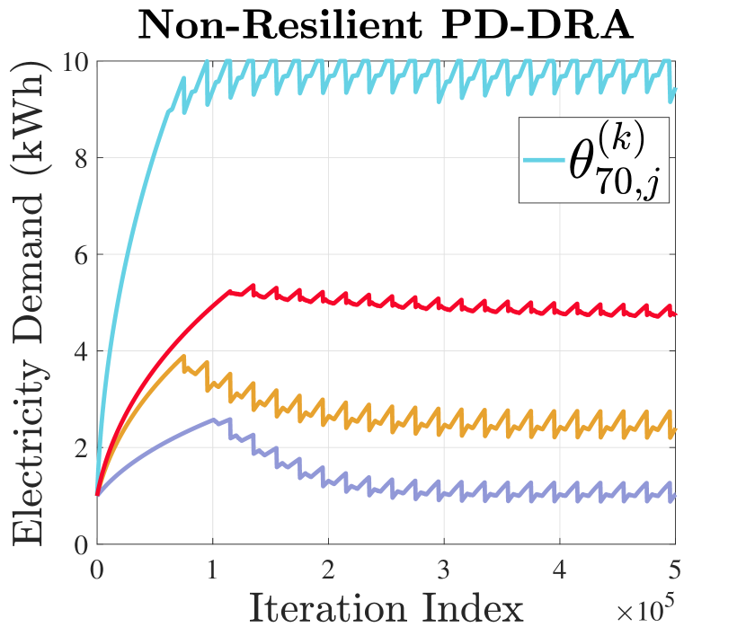
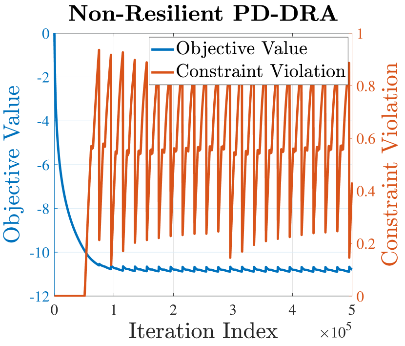
Figure 2: Illustration of basic PD-DRA algorithm failure under static impersonation attack. (a) The agents’ parameters do not converge, (b) the objective function does not converge and moreover there is constraint violation. We only display one constraint for brevity.

III-B Limitations of the Basic PD-DRA Algorithm

Applying the basic PD-DRA algorithm under a Byzantine attack scenario can lead to undesirable outcomes. Recall that the gradients in (5) depend on the average parameter 𝜽¯(k)superscript¯𝜽𝑘\overline{\bm{\theta}}^{(k)}. Under a Byzantine attack scenario, if the central coordinator forms the naive average 𝜽~(k)=(1/N)i=1N𝒓i(k)superscript~𝜽𝑘1𝑁superscriptsubscript𝑖1𝑁superscriptsubscript𝒓𝑖𝑘\widetilde{\bm{\theta}}^{(k)}=(1/N)\sum_{i=1}^{N}{\bm{r}}_{i}^{(k)} and computes the gradients gt(𝜽~(k))subscript𝑔𝑡superscript~𝜽𝑘\nabla g_{t}(\widetilde{\bm{\theta}}^{(k)}) accordingly, this may result in large error since the deviation 𝜽~(k)(1/N)i=1N𝜽i(k)superscript~𝜽𝑘1𝑁superscriptsubscript𝑖1𝑁superscriptsubscript𝜽𝑖𝑘\widetilde{\bm{\theta}}^{(k)}-(1/N)\sum_{i=1}^{N}\bm{\theta}_{i}^{(k)} can be large (proportional to the maximum diameter of 𝒞isubscript𝒞𝑖{\cal C}_{i}’s). This in turn can obstruct convergence and also overload the system by causing constraint violations.

Running Example (Basic PD-DRA Failure).

If the central coordinator believes all the agents are sending trustworthy information, then the optimal solution will occur when one agent is demanding 111kW and the others are demanding 666kW (so that the average is 555kW). But since the 111kW message is compromised and all the agents have same cost function, the compromised agent’s true electricity demand is also at a rate of 666kW. Hence, the solution delivers electricity at an average rate of 6kW, which is infeasible.

We preview our numerical result of applying the basic PD-DRA method under a static impersonation attack scenario for an optimal electric vehicle charging application in Figure 2. For constraint gt()subscript𝑔𝑡g_{t}(\cdot), we define constraint violation as max{0,gt(𝜽¯(k))}0subscript𝑔𝑡superscript¯𝜽𝑘\max\{0,g_{t}(\overline{\bm{\theta}}^{(k)})\}. Observe that the PD-DRA method does not provide convergence and the first constraint is being violated. From resource allocation perspective, this means that the agents are asking to consume more resources than the available amount in the system, which is infeasible. For details regarding the experimental setup, please see Section V.

IV Resilient PD-DRA Algorithms

Motivated by the failure of the basic PD-DRA procedure under Byzantine attack scenarios, resilient PD-DRA algorithms are necessary to optimize multi-agent systems in a distributed manner when the system is susceptible to attacks. We hold the following assumption to be true throughout the rest of the paper and propose two different attack resilient PD-DRA algorithms corresponding to the different attack scenarios outlined in Section III.

Assumption 1.

For all 𝛉d𝛉superscript𝑑\bm{\theta}\in\mathbb{R}^{d} and for all t𝑡t, the gradient of gtsubscript𝑔𝑡g_{t} is bounded with gt(𝛉)Bnormsubscript𝑔𝑡𝛉𝐵\|\nabla g_{t}(\bm{\theta})\|\leq B and is L𝐿L-Lipschitz continuous. Moreover, since maximum resource that can be consumed by an agent is bounded due to limited amount of resources, we let 𝟎𝒞i0subscript𝒞𝑖\bm{0}\in\mathcal{C}_{i} and upper bound the diameters of 𝒞isubscript𝒞𝑖\mathcal{C}_{i} by R:

max𝜽,𝜽𝒞i𝜽𝜽R,i=1,,N.formulae-sequencesubscript𝜽superscript𝜽subscript𝒞𝑖norm𝜽superscript𝜽𝑅𝑖1𝑁\max_{\bm{\theta},\bm{\theta}^{\prime}\in\mathcal{C}_{i}}\|\bm{\theta}-\bm{\theta}^{\prime}\|\leq R,~{}i=1,...,N. (10)
Running Example (Assumptions).

The constraint in our running example satisfies g(𝛉)=1𝑔𝛉1\nabla g(\bm{\theta})=1, which is bounded by B=1𝐵1B=1 and is L=0𝐿0L=0-Lipschitz continuous. Since the maximum charging rate is upper bounded by 777kW for three of the agents and by 101010kW for two of the agents, R=10𝑅10R=10.

IV-A Static Impersonation Attack

Under this attack scenario, given the complete lack of any credible information on the resource consumption parameters of the agents that permanently communicate through compromised channels, the central coordinator can only hope to solve the robust optimization model defined in (9) instead. This formulation considers a worst-case scenario on how much resources the compromised agents will consume, which ensures constraint satisfaction in all cases. However, the constraints in (9) require the knowledge of the set 𝒜𝒜\mathcal{A} and the sets 𝒞j,j𝒜subscript𝒞𝑗for-all𝑗𝒜\mathcal{C}_{j},\forall j\in\mathcal{A}, yet the central coordinator lacks this information.

Hence, in order to develop a robust optimization model that can handle the worst-case scenario without the knowledge of 𝒜𝒜\cal A, we let α1|𝒜|/Nsubscript𝛼1𝒜𝑁\alpha_{1}\geq|\mathcal{A}|/N as a known upper bound to the fraction of agents communicating through compromised channels and assume α1<1/2subscript𝛼112\alpha_{1}<1/2, where less than half of the agents are communicating through compromised channels.222If more than half of the agents communicate through compromised channels, then the adversary controls the majority and therefore the median, which will be used to estimate the average parameter later in the paper. In that case, there is no optimization based solution the central coordinator can implement in order to securely run the system. Let 𝜽¯:=1||i𝜽iassignsubscript¯𝜽1subscript𝑖subscript𝜽𝑖\overline{\bm{\theta}}_{\mathcal{H}}\vcentcolon=\frac{1}{|\mathcal{H}|}\sum_{i\in\mathcal{H}}\bm{\theta}_{i} be the mean of the agent’s parameters that are sent through trustworthy channels. We then define the following set of constraints

g¯t(𝜽):=gt(𝜽)+α1(RB+12LR2),assignsubscript¯𝑔𝑡𝜽subscript𝑔𝑡𝜽subscript𝛼1𝑅𝐵12𝐿superscript𝑅2\overline{g}_{t}(\bm{\theta})\vcentcolon=g_{t}(\bm{\theta})+\alpha_{1}\big{(}RB+{\textstyle\frac{1}{2}}LR^{2}\big{)}, (11)

and formulate a conservative approximation of (9):

Lemma 1.

Under Assumption 1 the following problem yields a conservative approximation of (9), i.e., its feasible set is a subset of the feasible set of (9):

min𝜽i𝒞i,iformulae-sequencesubscript𝜽𝑖subscript𝒞𝑖𝑖\displaystyle\underset{\bm{\theta}_{i}\in\mathcal{C}_{i},i\in\cal{H}}{\min} 1Nifi(𝜽i)1𝑁subscript𝑖subscript𝑓𝑖subscript𝜽𝑖\displaystyle\frac{1}{N}\sum_{i\in\cal{H}}{\color[rgb]{0,0,0}f_{i}}(\bm{\theta}_{i}) (12)
subject to g¯t((1α1)𝜽¯)0,t[T],formulae-sequencesubscript¯𝑔𝑡1subscript𝛼1subscript¯𝜽0for-all𝑡delimited-[]𝑇\displaystyle\overline{g}_{t}\left((1-\alpha_{1})\overline{\bm{\theta}}_{\mathcal{H}}\right)\leq 0,~{}\forall~{}t\in[T],

The proof can be found in Appendix -A.

Remark 2.

The proof of Lemma 1 is done by upper bounding constraints of (9) using Assumption 1 and the fact that α1|𝒜|/Nsubscript𝛼1𝒜𝑁\alpha_{1}\geq|{\cal A}|/N. The looser these upper bounds compared to the true values, the more conservative is (12). This approach potentially leaves less resources available to the agents communicating through trustworthy channels by assuming more than |𝒜|𝒜|{\cal A}| number of agents having maximum possible impact on the constraints, irrespective of their set 𝒞isubscript𝒞𝑖{\cal C}_{i} or the true value/gradient of the constraints.

Running Example (Conservative Approximation).

With B=1𝐵1B=1, L=0𝐿0L=0, and R=10𝑅10R=10, the conservative approximation of the running example has the following constraint:

g¯((1α1)𝜽¯)¯𝑔1subscript𝛼1subscript¯𝜽\displaystyle\overline{g}((1-\alpha_{1})\overline{\bm{\theta}}_{\cal H}) =g((1α1)𝜽¯)+α1(RB+12LR2)absent𝑔1subscript𝛼1subscript¯𝜽subscript𝛼1𝑅𝐵12𝐿superscript𝑅2\displaystyle=g((1-\alpha_{1})\overline{\bm{\theta}}_{\cal H})+\alpha_{1}(RB+\frac{1}{2}LR^{2})
=(1α1)𝜽¯5+10α1absent1subscript𝛼1subscript¯𝜽510subscript𝛼1\displaystyle=(1-\alpha_{1})\overline{\bm{\theta}}_{\cal H}-5+10\alpha_{1}

If α1=|𝒜|/N=0.2subscript𝛼1𝒜𝑁0.2\alpha_{1}=|{\cal A}|/N=0.2, then the upper bound is the fraction of compromised channels. In that case, the constraint is:

0.8𝜽¯30𝜽¯3.75,0.8subscript¯𝜽30subscript¯𝜽3.75\begin{split}0.8\overline{\bm{\theta}}_{\cal H}-3\leq 0\Leftrightarrow\overline{\bm{\theta}}_{\cal H}\leq 3.75,\end{split}

which is more conservative compared to the constraint of the robust optimization model (which was 𝛉¯4.5subscript¯𝛉4.5\overline{\bm{\theta}}_{\cal H}\leq 4.5). The optimal solution in this case is to deliver electricity at a rate of 3.753.753.75kW to the agents. The conservatism arises due to the difference between agent-specific maximum charging rate 777kW and the absolute maximum charging rate 101010kW. Since the constraint is linear, the gradient is constant. Hence, the smoothness and Lipschitz bounds hold with equality without causing additional conservatism.
If however α1=0.4subscript𝛼10.4\alpha_{1}=0.4, then the central coordinator assumes two agents communicating through compromised channels. In this case the conservative approximation has the constraint as

0.6𝜽¯10𝜽¯53,0.6subscript¯𝜽10subscript¯𝜽53\begin{split}0.6\overline{\bm{\theta}}_{\cal H}-1\leq 0\Leftrightarrow\overline{\bm{\theta}}_{\cal H}\leq\frac{5}{3},\end{split}

which results in charging at an even slower rate since the central coordinator has to be robust against two agents charging at the maximum rate of 101010kW.

To develop an attack resilient PD-DRA algorithm, we again define the regularized Lagrangian function of (12)italic-(12italic-)\eqref{eq:reformulate_s}:

¯υ({𝜽i}i;𝝀;):=1Nifi(𝜽i)+t=1Tλtg¯t((1α1)𝜽¯)+υ2Ni𝜽i2υ2𝝀2.assignsubscript¯𝜐subscriptsubscript𝜽𝑖𝑖𝝀1𝑁subscript𝑖subscript𝑓𝑖subscript𝜽𝑖superscriptsubscript𝑡1𝑇subscript𝜆𝑡subscript¯𝑔𝑡1subscript𝛼1subscript¯𝜽𝜐2𝑁subscript𝑖superscriptdelimited-∥∥subscript𝜽𝑖2𝜐2superscriptdelimited-∥∥𝝀2\begin{split}&\overline{\cal L}_{\upsilon}(\{\bm{\theta}_{i}\}_{i\in\cal{H}};\bm{\lambda};{\cal H})\\ &\vcentcolon={\textstyle\frac{1}{N}\sum_{i\in\cal{H}}}{\color[rgb]{0,0,0}f_{i}}(\bm{\theta}_{i})+{\textstyle\sum_{t=1}^{T}}\lambda_{t}\!~{}\overline{g}_{t}\left((1-\alpha_{1})\overline{\bm{\theta}}_{\mathcal{H}}\right)\\ &\hskip 14.22636pt\textstyle+\frac{\upsilon}{2N}\sum_{i\in\cal{H}}\|\bm{\theta}_{i}\|^{2}-\frac{\upsilon}{2}\|\bm{\lambda}\|^{2}.\end{split} (13)

The above function is (1α1)υ1subscript𝛼1𝜐(1-\alpha_{1})\upsilon-strongly convex and concave in 𝜽𝜽\bm{\theta} and 𝝀𝝀\bm{\lambda}, respectively (since (1α1)||N11subscript𝛼1𝑁1(1-\alpha_{1})\leq\textstyle{\frac{|\mathcal{H}|}{N}}\leq 1). Our main task is to tackle the following modified problem of (P) under Byzantine attack on (some of) the uplinks:

max𝝀+Tmin𝜽i𝒞i,i¯υ({𝜽i}i;𝝀;).subscript𝝀superscriptsubscript𝑇subscriptformulae-sequencesubscript𝜽𝑖subscript𝒞𝑖for-all𝑖subscript¯𝜐subscriptsubscript𝜽𝑖𝑖𝝀\max_{\bm{\lambda}\in\mathbb{R}_{+}^{T}}\min_{\bm{\theta}_{i}\in\mathcal{C}_{i},\forall i\in\cal{H}}~{}\overline{\cal L}_{\upsilon}(\{\bm{\theta}_{i}\}_{i\in\cal{H}};\bm{\lambda};{\cal H}). (Pυsubscriptsuperscriptabsent𝜐{}^{\prime}_{\upsilon})

Notice that (Pυsubscriptsuperscriptabsent𝜐{}^{\prime}_{\upsilon}) bears a similar form as (P) and thus one may apply the PD-DRA method to the former. The gradients with respect to primal/dual variables are given by:

𝜽i¯υ({𝜽i(k)}i;𝝀(k);)=1N(𝜽ifi(𝜽i(k))+υ𝜽i(k),+(1α1)N||t=1Tλt(k)𝜽g¯t(𝜽)|𝜽=(1α1)𝜽¯(k)),i,formulae-sequencesubscriptsubscript𝜽𝑖subscript¯𝜐subscriptsuperscriptsubscript𝜽𝑖𝑘𝑖superscript𝝀𝑘1𝑁subscriptsubscript𝜽𝑖subscript𝑓𝑖superscriptsubscript𝜽𝑖𝑘𝜐superscriptsubscript𝜽𝑖𝑘evaluated-at1subscript𝛼1𝑁superscriptsubscript𝑡1𝑇superscriptsubscript𝜆𝑡𝑘subscript𝜽subscript¯𝑔𝑡𝜽𝜽1subscript𝛼1superscriptsubscript¯𝜽𝑘for-all𝑖\begin{split}&\nabla_{\bm{\theta}_{i}}\overline{\cal L}_{\upsilon}(\{\bm{\theta}_{i}^{(k)}\}_{i\in\cal{H}};\bm{\lambda}^{(k)};{\cal H})=\frac{1}{N}\Big{(}\nabla_{\bm{\theta}_{i}}{\color[rgb]{0,0,0}f_{i}}(\bm{\theta}_{i}^{(k)})+\upsilon\!~{}\bm{\theta}_{i}^{(k)},\\ &\textstyle+\frac{(1-\alpha_{1})N}{|\mathcal{H}|}\sum_{t=1}^{T}\lambda_{t}^{(k)}\nabla_{\bm{\theta}}\overline{g}_{t}(\bm{\theta})\Big{|}_{\bm{\theta}=(1-\alpha_{1})\bar{\bm{\theta}}_{\mathcal{H}}^{(k)}}\Big{)},{\color[rgb]{0,0,0}\forall i\in{\cal H}},\\ \end{split} (14a)
[𝝀¯υ({𝜽i(k)}i;𝝀(k);)]t=g¯t((1α1)𝜽¯(k))υλt(k).subscriptdelimited-[]subscript𝝀subscript¯𝜐subscriptsuperscriptsubscript𝜽𝑖𝑘𝑖superscript𝝀𝑘𝑡subscript¯𝑔𝑡1subscript𝛼1subscriptsuperscript¯𝜽𝑘𝜐superscriptsubscript𝜆𝑡𝑘\begin{split}&\big{[}\nabla_{\bm{\lambda}}\overline{\cal L}_{\upsilon}(\{\bm{\theta}_{i}^{(k)}\}_{i\in\cal{H}};\bm{\lambda}^{(k)};{\cal H})\big{]}_{t}=\overline{g}_{t}\Big{(}(1-\alpha_{1})\overline{\bm{\theta}}^{(k)}_{\mathcal{H}}\Big{)}-\upsilon\lambda_{t}^{(k)}.\end{split} (14b)

However, such application requires the central coordinator to compute the sample average

𝜽¯(k)=1||i𝜽i(k),subscriptsuperscript¯𝜽𝑘1subscript𝑖superscriptsubscript𝜽𝑖𝑘\textstyle\overline{\bm{\theta}}^{(k)}_{\cal H}=\frac{1}{|{\cal H}|}\sum_{i\in{\cal H}}\bm{\theta}_{i}^{(k)}, (15)

at each iteration. The above might not be computationally feasible under the attack model, since the central coordinator is oblivious to the identity of {\cal H}. As a solution, the central coordinator computes the robust mean 𝜽^(k)superscriptsubscript^𝜽𝑘\widehat{\bm{\theta}}_{\mathcal{H}}^{(k)} of the received parameters {𝒓i(k)}i[N]subscriptsuperscriptsubscript𝒓𝑖𝑘𝑖delimited-[]𝑁\{\bm{r}_{i}^{(k)}\}_{i\in[N]} using a median-based mean estimator described next.

IV-A1 Overview of Median-Based Mean Estimation

Consider a set of N𝑁N vectors {𝒙id}i=1Nsuperscriptsubscriptsubscript𝒙𝑖superscript𝑑𝑖1𝑁\{{\bm{x}}_{i}\in\mathbb{R}^{d}\}_{i=1}^{N}, among which at least (1α1)N1subscript𝛼1𝑁(1-\alpha_{1})N are trustworthy (𝒙isubscript𝒙𝑖\bm{x}_{i}\in\mathcal{H}) and at most α1Nsubscript𝛼1𝑁\alpha_{1}N are compromised (𝒙i𝒜subscript𝒙𝑖𝒜\bm{x}_{i}\in\mathcal{A}). We consider a simple median-based estimator applied to each coordinate j=1,,d𝑗1𝑑j=1,\dots,d. First, define the coordinate-wise median as:

[𝒙𝗆𝖾𝖽]j=𝗆𝖾𝖽({[𝒙i]j}i=1N),subscriptdelimited-[]subscript𝒙𝗆𝖾𝖽𝑗𝗆𝖾𝖽superscriptsubscriptsubscriptdelimited-[]subscript𝒙𝑖𝑗𝑖1𝑁\left[{\bm{x}}_{\sf med}\right]_{j}={\sf med}\left(\{[{\bm{x}}_{i}]_{j}\}_{i=1}^{N}\right),

where 𝗆𝖾𝖽()𝗆𝖾𝖽{\sf med(\cdot)} computes the median of the operand. Then, our estimator is computed as the mean of the nearest (1α1)N1subscript𝛼1𝑁(1-\alpha_{1})N neighbors of [𝒙𝗆𝖾𝖽]jsubscriptdelimited-[]subscript𝒙𝗆𝖾𝖽𝑗\left[{\bm{x}}_{\sf med}\right]_{j}. Our estimator is:

[𝒙^]j=1(1α1)Ni𝒩j[𝒙i]j,subscriptdelimited-[]subscript^𝒙𝑗11subscript𝛼1𝑁subscript𝑖subscript𝒩𝑗subscriptdelimited-[]subscript𝒙𝑖𝑗\textstyle[\widehat{\bm{x}}_{\mathcal{H}}]_{j}=\frac{1}{(1-\alpha_{1})N}\sum_{i\in{\cal N}_{j}}[{\bm{x}}_{i}]_{j}, (16)

where we have defined the set with |𝒩j|=(1α1)Nsubscript𝒩𝑗1subscript𝛼1𝑁|{\cal N}_{j}|=(1-\alpha_{1})N as:

𝒩j={i[N]:|[𝒙i𝒙𝗆𝖾𝖽]j|rj},subscript𝒩𝑗conditional-set𝑖delimited-[]𝑁subscriptdelimited-[]subscript𝒙𝑖subscript𝒙𝗆𝖾𝖽𝑗subscript𝑟𝑗{\color[rgb]{0,0,0}{\cal N}_{j}}=\{i\in[N]:\big{|}\big{[}{\bm{x}}_{i}-{\bm{x}}_{\sf med}\big{]}_{j}\big{|}\leq r_{j}\},

such that rjsubscript𝑟𝑗r_{j} is chosen to satisfy |𝒩j|=(1α1)Nsubscript𝒩𝑗1subscript𝛼1𝑁|{\cal N}_{j}|=(1-\alpha_{1})N.

The following bounds the performance of (16):

Proposition 2.

Let 𝐱¯subscript¯𝐱\overline{\bm{x}}_{\mathcal{H}} be the mean of the trustworthy vectors. Suppose that maxi𝐱i𝐱¯rsubscript𝑖subscriptnormsubscript𝐱𝑖subscript¯𝐱𝑟\max_{i\in{\cal H}}\|\bm{x}_{i}-\overline{\bm{x}}_{\cal H}\|_{\infty}\leq r, then for any α1(0,12)subscript𝛼1012\alpha_{1}\in(0,\frac{1}{2}), it holds that:

𝒙^𝒙¯2α11α1(1+(1α1)212α1)rd.normsubscript^𝒙subscript¯𝒙2subscript𝛼11subscript𝛼11superscript1subscript𝛼1212subscript𝛼1𝑟𝑑\|\widehat{\bm{x}}_{\cal H}-\overline{\bm{x}}_{\cal H}\|\leq\frac{2\alpha_{1}}{1-\alpha_{1}}\left(1+\sqrt{\frac{(1-\alpha_{1})^{2}}{1-2\alpha_{1}}}\right)r\sqrt{d}. (17)

The proof can be found in Appendix -B. We note that for sufficiently small α1subscript𝛼1\alpha_{1}, the right hand side on (17) can be approximated by 𝒪(α1rd)𝒪subscript𝛼1𝑟𝑑{\cal O}(\alpha_{1}r\sqrt{d}). Using this median-based mean estimator, we propose the robust PD-DRA algorithm as follows.

1:  Input: Each agent has initial state 𝜽i(0)superscriptsubscript𝜽𝑖0\bm{\theta}_{i}^{(0)}.
2:  for k=1,2,𝑘12k=1,2,... do
3:      (At the Central Coordinator):
  1. (a)

    Receives {𝒓i(k)}i=1Nsuperscriptsubscriptsuperscriptsubscript𝒓𝑖𝑘𝑖1𝑁\{{\bm{r}}_{i}^{(k)}\}_{i=1}^{N}, see (8), from agents.

  2. (b)

    Computes robust mean 𝜽^(k)superscriptsubscript^𝜽𝑘\widehat{\bm{\theta}}_{\cal H}^{(k)} using the estimator (16).

  3. (c)

    Broadcasts the vector 𝒈^(k):=t=1Tλt(k)𝜽g¯t((1α1)𝜽^(k))assignsubscriptsuperscript^𝒈𝑘superscriptsubscript𝑡1𝑇superscriptsubscript𝜆𝑡𝑘subscript𝜽subscript¯𝑔𝑡1subscript𝛼1superscriptsubscript^𝜽𝑘\widehat{\bm{g}}^{(k)}_{\cal H}\vcentcolon=\sum_{t=1}^{T}\lambda_{t}^{(k)}\nabla_{\bm{\theta}}\overline{g}_{t}((1-\alpha_{1})\widehat{\bm{\theta}}_{\cal H}^{(k)}) to agents.

  4. (d)

    Computes the update for 𝝀(k+1)superscript𝝀𝑘1\bm{\lambda}^{(k+1)} with (18b).

4:      (At each agent i𝑖i{\color[rgb]{0,0,0}\in\mathcal{H}}):
  1. (a)

    Agent receives 𝒈^(k)subscriptsuperscript^𝒈𝑘\widehat{\bm{g}}^{(k)}_{\cal H}.

  2. (b)

    Agent computes update for 𝜽i(k+1)superscriptsubscript𝜽𝑖𝑘1\bm{\theta}_{i}^{(k+1)} with (18a).

5:  end for
Algorithm 2 Robust PD-DRA Algorithm

IV-A2 Robust PD-DRA Algorithm

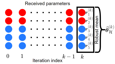
We summarize the static impersonation attack resilient PD-DRA method in Algorithm 2. The algorithm behaves similarly as Algorithm 1 applied to (Pυsubscriptsuperscriptabsent𝜐{}^{\prime}_{\upsilon}), with the exception that the central coordinator is oblivious to {\cal H}, and it uses a robust mean estimator to find an approximate average for the signals sent through the trustworthy links, as illustrated in Figure 3. This approximate value is used to compute the new price signals, and sent back to agents. In particular, the primal-dual updates are:

𝜽i(k+1)=𝒫𝒞i(𝜽i(k)γN(𝒈^(k)+𝜽ifi(𝜽i(k))+υ𝜽i(k))),superscriptsubscript𝜽𝑖𝑘1subscript𝒫subscript𝒞𝑖superscriptsubscript𝜽𝑖𝑘𝛾𝑁subscriptsuperscript^𝒈𝑘subscriptsubscript𝜽𝑖subscript𝑓𝑖superscriptsubscript𝜽𝑖𝑘𝜐superscriptsubscript𝜽𝑖𝑘\bm{\theta}_{i}^{(k+1)}={\cal P}_{\mathcal{C}_{i}}\big{(}\bm{\theta}_{i}^{(k)}-{\textstyle\frac{\gamma}{N}}\big{(}\widehat{\bm{g}}^{(k)}_{\cal H}+\nabla_{\bm{\theta}_{i}}{\color[rgb]{0,0,0}f_{i}}(\bm{\theta}_{i}^{(k)})+\upsilon\bm{\theta}_{i}^{(k)}\big{)}\big{)}, (18a)
λt(k+1)=[λt(k)+γ(g¯t((1α1)𝜽^(k))υλt(k))]+.superscriptsubscript𝜆𝑡𝑘1subscriptdelimited-[]superscriptsubscript𝜆𝑡𝑘𝛾subscript¯𝑔𝑡1subscript𝛼1superscriptsubscript^𝜽𝑘𝜐superscriptsubscript𝜆𝑡𝑘\lambda_{t}^{(k+1)}=\big{[}\lambda_{t}^{(k)}+\gamma\big{(}\overline{g}_{t}((1-\alpha_{1})\widehat{\bm{\theta}}_{\cal H}^{(k)})-\upsilon\lambda_{t}^{(k)}\big{)}\big{]}_{+}. (18b)

We note that the update rule in (18a) is valid for agents in set {\cal H}, because the gradients of the Lagrangian are defined only for those agents in (14a). The agents in set 𝒜𝒜\cal A may or may not use the same update rule, however, this does not have any impact on the algorithm as they can never communicate their true parameters to the central coordinator.

Lemma 2.

Algorithm 2 is a primal-dual algorithm [10] for (Pυsubscriptsuperscriptabsentitalic-′𝜐{}^{\prime}_{\upsilon}) with perturbed gradients:

𝒈^𝜽(k)superscriptsubscript^𝒈𝜽𝑘\displaystyle\widehat{\bm{g}}_{\bm{\theta}}^{(k)} =𝜽¯υ(𝜽(k);𝝀(k);)+𝒆𝜽(k),absentsubscript𝜽subscript¯𝜐superscript𝜽𝑘superscript𝝀𝑘superscriptsubscript𝒆𝜽𝑘\displaystyle=\nabla_{\bm{\theta}}\overline{\cal L}_{\upsilon}(\bm{\theta}^{(k)};\bm{\lambda}^{(k)};{\cal H})+{\bm{e}}_{\bm{\theta}}^{(k)}, (19a)
𝒈^𝝀(k)superscriptsubscript^𝒈𝝀𝑘\displaystyle\widehat{\bm{g}}_{\bm{\lambda}}^{(k)} =𝝀¯υ(𝜽(k);𝝀(k);)+𝒆𝝀(k),absentsubscript𝝀subscript¯𝜐superscript𝜽𝑘superscript𝝀𝑘superscriptsubscript𝒆𝝀𝑘\displaystyle=\nabla_{\bm{\lambda}}\overline{\cal L}_{\upsilon}(\bm{\theta}^{(k)};\bm{\lambda}^{(k)};{\cal H})+{\bm{e}}_{\bm{\lambda}}^{(k)}, (19b)

where we have used concatenated variable as 𝛉=({𝛉i}i)𝛉subscriptsubscript𝛉𝑖𝑖\bm{\theta}=(\{\bm{\theta}_{i}\}_{i\in\cal{H}}). Under Assumption 1 and assuming that λt(k)λ¯superscriptsubscript𝜆𝑡𝑘¯𝜆\lambda_{t}^{(k)}\leq\overline{\lambda} for all k𝑘k, we have:

𝒆𝜽(k)normsuperscriptsubscript𝒆𝜽𝑘absent\displaystyle\|{\bm{e}}_{\bm{\theta}}^{(k)}\|\leq (1α1)λ¯LT𝜽^(k)𝜽¯(k)1subscript𝛼1¯𝜆𝐿𝑇normsuperscriptsubscript^𝜽𝑘superscriptsubscript¯𝜽𝑘\displaystyle(1-\alpha_{1})\overline{\lambda}LT\|\widehat{\bm{\theta}}_{\cal H}^{(k)}-\overline{\bm{\theta}}_{\cal H}^{(k)}\| (20)
+||(1α1)N||λ¯BT,1subscript𝛼1𝑁¯𝜆𝐵𝑇\displaystyle+\frac{|\mathcal{H}|-(1-\alpha_{1})N}{|\mathcal{H}|}\overline{\lambda}BT,
𝒆𝝀(k)(1α1)BT𝜽^(k)𝜽¯(k).normsuperscriptsubscript𝒆𝝀𝑘1subscript𝛼1𝐵𝑇normsuperscriptsubscript^𝜽𝑘superscriptsubscript¯𝜽𝑘\|{\bm{e}}_{\bm{\lambda}}^{(k)}\|\leq(1-\alpha_{1})BT\|\widehat{\bm{\theta}}_{\cal H}^{(k)}-\overline{\bm{\theta}}_{\cal H}^{(k)}\|. (21)

The proof can be found in Appendix -C. The assumption λt(k)λ¯superscriptsubscript𝜆𝑡𝑘¯𝜆\lambda_{t}^{(k)}\leq\overline{\lambda} can be guaranteed since g¯t((1α1)𝜽^(k))subscript¯𝑔𝑡1subscript𝛼1superscriptsubscript^𝜽𝑘\overline{g}_{t}((1-\alpha_{1})\widehat{\bm{\theta}}_{\cal H}^{(k)}) is bounded, which is proven in Appendix -H. Furthermore, the performance analysis for the median based estimator shows that

𝜽^(k)𝜽¯(k)=𝒪(α1Rd)normsuperscriptsubscript^𝜽𝑘superscriptsubscript¯𝜽𝑘𝒪subscript𝛼1𝑅𝑑\|\widehat{\bm{\theta}}_{\cal H}^{(k)}-\overline{\bm{\theta}}_{\cal H}^{(k)}\|={\cal O}(\alpha_{1}R\sqrt{d}) (22)

when α1subscript𝛼1\alpha_{1} is small. Finally, based on Lemma 2, we can analyze the convergence of Algorithm 2. Let 𝒛^=(𝜽^,𝝀^)superscript^𝒛superscript^𝜽superscript^𝝀\widehat{\bm{z}}^{\star}=(\widehat{\bm{\theta}}^{\star},\widehat{\bm{\lambda}}^{\star}) be a saddle point of (Pυsubscriptsuperscriptabsent𝜐{}^{\prime}_{\upsilon}) and define

𝚽¯(𝒛(k)):=(𝜽¯υ({𝜽i(k)}i,𝝀(k);)𝝀¯υ({𝜽i(k)}i,𝝀(k);)).assign¯𝚽superscript𝒛𝑘subscript𝜽subscript¯𝜐subscriptsuperscriptsubscript𝜽𝑖𝑘𝑖superscript𝝀𝑘subscript𝝀subscript¯𝜐subscriptsuperscriptsubscript𝜽𝑖𝑘𝑖superscript𝝀𝑘\overline{\bm{\Phi}}({\bm{z}}^{(k)})\vcentcolon=\left(\begin{array}[]{c}\nabla_{\bm{\theta}}\overline{\cal L}_{\upsilon}(\{\bm{\theta}_{i}^{(k)}\}_{i\in\cal{H}},\bm{\lambda}^{(k)};{\cal H})\\ -\nabla_{\bm{\lambda}}\overline{\cal L}_{\upsilon}(\{\bm{\theta}_{i}^{(k)}\}_{i\in\cal{H}},\bm{\lambda}^{(k)};{\cal H})\end{array}\right). (23)

We are ready to present our main result for static attacks.
Refer to caption
Figure 3: Robust mean estimation under static impersonation attack. Red/blue circles correspond to parameters received through compromised/trustworthy channels, respectively. In this example, there are N=5𝑁5N=5 agents and agents 1 and 2 are always communicating through compromised channels. At iteration k𝑘k, the central coordinator computes the robust mean 𝜽^(k)subscriptsuperscript^𝜽𝑘\widehat{\bm{\theta}}^{(k)}_{\cal H} of the received parameters {𝒓i(k)}i[N]subscriptsuperscriptsubscript𝒓𝑖𝑘𝑖delimited-[]𝑁\{\bm{r}_{i}^{(k)}\}_{i\in[N]}.
Theorem 1.

Assume the map 𝚽¯(𝐳(k))¯𝚽superscript𝐳𝑘\overline{\bm{\Phi}}({\bm{z}}^{(k)}) is LΦsubscript𝐿ΦL_{\Phi}-Lipschitz continuous. For Algorithm 2, for all k0𝑘0k\geq 0 it holds:

𝒛(k+1)𝒛^2(1γυ+2γ2LΦ2)𝒛(k)𝒛^2+(4γυ+2γ2)Ek.superscriptdelimited-∥∥superscript𝒛𝑘1superscript^𝒛21𝛾superscript𝜐2superscript𝛾2superscriptsubscript𝐿Φ2superscriptdelimited-∥∥superscript𝒛𝑘superscript^𝒛24𝛾superscript𝜐2superscript𝛾2subscript𝐸𝑘\begin{split}\|{\bm{z}}^{(k+1)}-\widehat{\bm{z}}^{\star}\|^{2}\leq&\big{(}1-\gamma\upsilon^{\prime}+2\gamma^{2}L_{\Phi}^{2}\big{)}\|{\bm{z}}^{(k)}-\widehat{\bm{z}}^{\star}\|^{2}\\ &+\left(\frac{4\gamma}{\upsilon^{\prime}}+2\gamma^{2}\right)E_{k}.\end{split} (24)

where υ:=(1α1)υassignsuperscript𝜐1subscript𝛼1𝜐\upsilon^{\prime}\vcentcolon=(1-\alpha_{1})\upsilon and Ek:=𝐞𝛉(k)2+𝐞𝛌(k)2assignsubscript𝐸𝑘superscriptnormsuperscriptsubscript𝐞𝛉𝑘2superscriptnormsuperscriptsubscript𝐞𝛌𝑘2E_{k}\vcentcolon=\|{\bm{e}}_{\bm{\theta}}^{(k)}\|^{2}+\|{\bm{e}}_{\bm{\lambda}}^{(k)}\|^{2} is the total perturbation at iteration k𝑘k. Moreover, if we choose γ<υ/2LΦ2𝛾superscript𝜐2superscriptsubscript𝐿Φ2\gamma<{\upsilon^{\prime}}/{2L_{\Phi}^{2}} and Eksubscript𝐸𝑘E_{k} is upper bounded by E¯¯𝐸\overline{E} for all k𝑘k, then

lim supk𝒛(k)𝒛^24υ+2γυ2γLΦ2E¯.subscriptlimit-supremum𝑘superscriptnormsuperscript𝒛𝑘superscript^𝒛24superscript𝜐2𝛾superscript𝜐2𝛾superscriptsubscript𝐿Φ2¯𝐸\limsup_{k\rightarrow\infty}\|{\bm{z}}^{(k)}-\widehat{\bm{z}}^{\star}\|^{2}\leq\frac{\frac{4}{\upsilon^{\prime}}+2\gamma}{\upsilon^{\prime}-2\gamma L_{\Phi}^{2}}\overline{E}. (25)

The proof can be found in Appendix -D. Combining with (22) shows that the resilient PD-DRA method converges to a 𝒪(α12R2d)𝒪superscriptsubscript𝛼12superscript𝑅2𝑑{\cal O}(\alpha_{1}^{2}R^{2}d) neighborhood of the saddle point of (Pυsubscriptsuperscriptabsent𝜐{}^{\prime}_{\upsilon}). Moreover, it shows that the convergence rate to the neighborhood is linear, which is similar to the classical analysis in [10].

IV-B Dynamic Impersonation Attack

Under this attack scenario, the set of agents communicating through compromised channels is dynamically changing with iterations. We make the following assumption on how frequently each agent’s communications are compromised:

Assumption 2.

Let m𝑚m be a fixed window size and α2<0.5subscript𝛼20.5\alpha_{2}<0.5 be a known upper bound on how frequent an agent communicates through a compromised channel. Then, for all km1𝑘𝑚1k\geq m-1 and for all agents i[N]𝑖delimited-[]𝑁i\in[N], among the received parameters {𝐫i(k)}=0m1superscriptsubscriptsuperscriptsubscript𝐫𝑖𝑘0𝑚1\{\bm{r}_{i}^{(k-\ell)}\}_{\ell=0}^{m-1} at most α2msubscript𝛼2𝑚\alpha_{2}m are sent through compromised channels.

It is important to recall that the dynamic attack scenario does not generalize the static attack scenario and there is a significant distinction between the two. The static attack scenario assumes that a fixed set of agents’ communications are permanently compromised. It may occur when when the attacker compromises set of communication channels and those channels are assigned to the agents via a static channel allocation scheme.

On the contrary, for the dynamic attack scenario, each user’s communications are vulnerable to attacks for at most a given α2subscript𝛼2\alpha_{2} fraction of iterations over a window of size m𝑚m under Assumption 2, and hence each agent is able to communicate reliably with the central coordinator at some iterations. This scheme may occur when the attacker compromises a fixed set of communication channels (same as the static scenario), however, the channels are assigned to the agents via a dynamic channel allocation scheme (e.g., do a round-robin channel allocation. If there are m𝑚m communication channels out of which α2msubscript𝛼2𝑚\alpha_{2}m are compromised, assigning channels dynamically in a cyclic way to the agents ensures that over a window of m𝑚m, every agent has sent α2msubscript𝛼2𝑚\alpha_{2}m compromised messages). Although the attacker behaves the same way, we can simulate both scenarios by static/dynamic channel allocation. In cyber-physical systems, such dynamic allocation schemes are commonly used (e.g., dynamic IP assignment to be protected from hackers).

Interestingly, it is possible to develop an algorithm that converges to the optimal solution of Problem (Pυ). The intuition behind is that the received parameters over a long period of time contain a fraction of trustworthy information that can extracted by the algorithm to perform faithful computations.

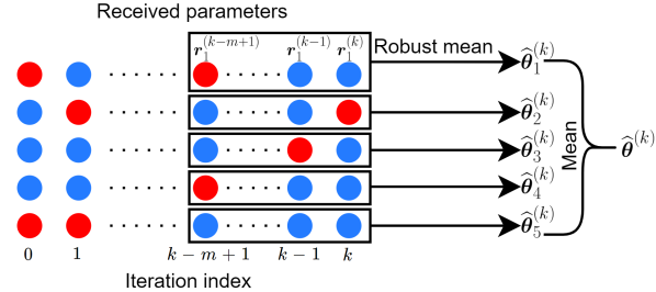
Our algorithm is similar in nature to an averaging gradient scheme where the primal-dual updates utilize the averages of time delayed gradients. Furthermore, the scheme is combined with the robust mean estimator developed in Sec. IV-A1 to approximate the averages of outdated gradients, as illustrated in Figure 4. Specifically, the central coordinator chooses a window size of m𝑚m. For any iteration km1𝑘𝑚1k\geq m-1, instead of using 𝒓i(k)superscriptsubscript𝒓𝑖𝑘\bm{r}_{i}^{(k)} for computing the average parameter 𝜽¯(k)superscript¯𝜽𝑘\overline{\bm{\theta}}^{(k)} and the gradients, the central coordinator computes the robust mean 𝜽^i(k)superscriptsubscript^𝜽𝑖𝑘\widehat{\bm{\theta}}_{i}^{(k)} from the received parameters {𝒓i(k)}=0m1superscriptsubscriptsuperscriptsubscript𝒓𝑖𝑘0𝑚1\{\bm{r}_{i}^{(k-\ell)}\}_{\ell=0}^{m-1} using the median-based mean estimator (16) for all agents i[N]𝑖delimited-[]𝑁i\in[N], applied on the sequence of historical received parameters. Note that we have replaced α1subscript𝛼1\alpha_{1} by α2subscript𝛼2\alpha_{2}, N𝑁N by m𝑚m in this application. It then uses 𝜽^(k):=1Ni=1N𝜽^i(k)assignsuperscript^𝜽𝑘1𝑁superscriptsubscript𝑖1𝑁superscriptsubscript^𝜽𝑖𝑘\widehat{\bm{\theta}}^{(k)}\vcentcolon=\frac{1}{N}\sum_{i=1}^{N}\widehat{\bm{\theta}}_{i}^{(k)} for computation of the primal-dual updates.
Refer to caption
Figure 4: Robust mean estimation under dynamic impersonation attacks. Red/blue circles correspond to parameters received through compromised/trustworthy channels, respectively. In this example, there are N=5𝑁5N=5 agents and the set of agents communicating through compromised channels is changing at every iteration. At iteration k𝑘k, the central coordinator computes the robust mean 𝜽^i(k)superscriptsubscript^𝜽𝑖𝑘\widehat{\bm{\theta}}_{i}^{(k)} of the received parameters {𝒓i(k)}=0m1superscriptsubscriptsuperscriptsubscript𝒓𝑖𝑘0𝑚1\{\bm{r}_{i}^{(k-\ell)}\}_{\ell=0}^{m-1} for all agents i[N]𝑖delimited-[]𝑁i\in[N]. Then, computes the naive average of {𝜽^i(k)}i=1Nsuperscriptsubscriptsuperscriptsubscript^𝜽𝑖𝑘𝑖1𝑁\{\widehat{\bm{\theta}}_{i}^{(k)}\}_{i=1}^{N} to get the average parameter 𝜽^(k)superscript^𝜽𝑘\widehat{\bm{\theta}}^{(k)}.

We summarize our robust averaging PD-DRA method in Algorithm 3. The primal-dual updates are described by:

𝜽i(k+1)=𝒫𝒞i(𝜽i(k)γN(𝒈^(k)+𝜽ifi(𝜽i(k))+υ𝜽i(k))),superscriptsubscript𝜽𝑖𝑘1subscript𝒫subscript𝒞𝑖superscriptsubscript𝜽𝑖𝑘𝛾𝑁superscript^𝒈𝑘subscriptsubscript𝜽𝑖subscript𝑓𝑖superscriptsubscript𝜽𝑖𝑘𝜐superscriptsubscript𝜽𝑖𝑘\bm{\theta}_{i}^{(k+1)}={\cal P}_{\mathcal{C}_{i}}\big{(}\bm{\theta}_{i}^{(k)}-{\textstyle\frac{\gamma}{N}}\big{(}\widehat{\bm{g}}^{(k)}+\nabla_{\bm{\theta}_{i}}{\color[rgb]{0,0,0}f_{i}}(\bm{\theta}_{i}^{(k)})+\upsilon\bm{\theta}_{i}^{(k)}\big{)}\big{)}, (26a)
λt(k+1)=[λt(k)+γ(gt(𝜽^(k))υλt(k))]+.superscriptsubscript𝜆𝑡𝑘1subscriptdelimited-[]superscriptsubscript𝜆𝑡𝑘𝛾subscript𝑔𝑡superscript^𝜽𝑘𝜐superscriptsubscript𝜆𝑡𝑘\lambda_{t}^{(k+1)}=\big{[}\lambda_{t}^{(k)}+\gamma\big{(}g_{t}({\textstyle\widehat{\bm{\theta}}^{(k)})-\upsilon\lambda_{t}^{(k)}\big{)}\big{]}_{+}}. (26b)
Lemma 3.

Algorithm 3 is a primal-dual algorithm for (Pυ) with perturbed gradients:

𝒈^𝜽(k)=𝜽υ(𝜽(k);𝝀(k))+𝒆𝜽(k),subscriptsuperscriptbold-^𝒈𝑘𝜽subscript𝜽subscript𝜐superscript𝜽𝑘superscript𝝀𝑘superscriptsubscript𝒆𝜽𝑘\displaystyle\bm{\widehat{g}}^{(k)}_{\bm{\theta}}=\nabla_{\bm{\theta}}\mathcal{L}_{\upsilon}(\bm{\theta}^{(k)};\bm{\lambda}^{(k)})+\bm{e}_{\bm{\theta}}^{(k)}, (27a)
𝒈^𝝀(k)=𝝀υ(𝜽(k);𝝀(k))+𝒆𝝀(k),subscriptsuperscriptbold-^𝒈𝑘𝝀subscript𝝀subscript𝜐superscript𝜽𝑘superscript𝝀𝑘superscriptsubscript𝒆𝝀𝑘\displaystyle\bm{\widehat{g}}^{(k)}_{\bm{\lambda}}=\nabla_{\bm{\lambda}}\mathcal{L}_{\upsilon}(\bm{\theta}^{(k)};\bm{\lambda}^{(k)})+\bm{e}_{\bm{\lambda}}^{(k)}, (27b)

where we have used concatenated variable as 𝛉=({𝛉i}iN)𝛉subscriptsubscript𝛉𝑖𝑖𝑁\bm{\theta}=(\{\bm{\theta}_{i}\}_{i\in N}). Under Assumption 1 and assuming that λt(k)λ¯superscriptsubscript𝜆𝑡𝑘¯𝜆\lambda_{t}^{(k)}\leq\overline{\lambda} for all k, we have:

𝒆𝜽(k)λ¯LTNi=1N𝜽i(k)𝜽^i(k),\displaystyle\|\bm{e}^{(k)}_{\bm{\theta}}\|\leq\frac{\overline{\lambda}LT}{N}\sum_{i=1}^{N}\|\bm{\theta}_{i}^{(k)}-\widehat{\bm{\theta}}{}_{i}^{(k)}\|, (28a)
𝒆𝝀(k)BTNi=1N𝜽i(k)𝜽^i(k).\displaystyle\|\bm{e}^{(k)}_{\bm{\lambda}}\|\leq\frac{BT}{N}\sum_{i=1}^{N}\|\bm{\theta}_{i}^{(k)}-\widehat{\bm{\theta}}{}_{i}^{(k)}\|. (28b)
1:  Input: Each agent has initial state 𝜽i(0)superscriptsubscript𝜽𝑖0\bm{\theta}_{i}^{(0)}.
2:  for k=0,1,,m2𝑘01𝑚2k=0,1,\dots,m-2 do
3:     Apply basic PD-DRA (Run Algorithm 1).
4:  end for
5:  for k=m1,m,𝑘𝑚1𝑚k=m-1,m,\dots do
6:     (At the Central Coordinator):
  1. (a)

    Receives {𝒓i(k)}i=1Nsuperscriptsubscriptsuperscriptsubscript𝒓𝑖𝑘𝑖1𝑁\{{\bm{r}}_{i}^{(k)}\}_{i=1}^{N}, see (8), from agents.

  2. (b)

    For all agents i=1,,N𝑖1𝑁i=1,\dots,N, computes robust mean 𝜽^i(k)superscriptsubscript^𝜽𝑖𝑘\widehat{\bm{\theta}}_{i}^{(k)} of {𝒓i(k)}=0m1superscriptsubscriptsuperscriptsubscript𝒓𝑖𝑘0𝑚1\{\bm{r}_{i}^{(k-\ell)}\}_{\ell=0}^{m-1} using the estimator (16) with parameters α1α2subscript𝛼1subscript𝛼2\alpha_{1}\rightarrow\alpha_{2}, Nm𝑁𝑚N\rightarrow m.

  3. (c)

    Computes 𝜽^(k):=1Ni=1N𝜽^i(k)assignsuperscript^𝜽𝑘1𝑁superscriptsubscript𝑖1𝑁subscriptsuperscript^𝜽𝑘𝑖\widehat{\bm{\theta}}^{(k)}\vcentcolon=\frac{1}{N}\sum_{i=1}^{N}\widehat{\bm{\theta}}^{(k)}_{i}.

  4. (d)

    Broadcasts the vector 𝒈^(k):=t=1Tλt(k)𝜽gt(𝜽^(k))assignsuperscript^𝒈𝑘superscriptsubscript𝑡1𝑇superscriptsubscript𝜆𝑡𝑘subscript𝜽subscript𝑔𝑡superscript^𝜽𝑘\widehat{\bm{g}}^{(k)}\vcentcolon=\sum_{t=1}^{T}\lambda_{t}^{(k)}\nabla_{\bm{\theta}}g_{t}(\widehat{\bm{\theta}}^{(k)}) to agents.

  5. (e)

    Computes the update for 𝝀(k+1)superscript𝝀𝑘1\bm{\lambda}^{(k+1)} with (26b).

7:     (At each agent i𝑖i):
  1. (a)

    Agent receives 𝒈^(k)superscript^𝒈𝑘\widehat{\bm{g}}^{(k)}.

  2. (b)

    Agent computes update for 𝜽i(k+1)superscriptsubscript𝜽𝑖𝑘1\bm{\theta}_{i}^{(k+1)} with (26a).

8:  end for
Algorithm 3 Averaging PD-DRA Algorithm

The proof can be found in Appendix -E. The assumption λt(k)λ¯superscriptsubscript𝜆𝑡𝑘¯𝜆\lambda_{t}^{(k)}\leq\overline{\lambda} can be guaranteed since gt(𝜽^(k))subscript𝑔𝑡superscript^𝜽𝑘g_{t}(\widehat{\bm{\theta}}^{(k)}) is bounded, which is proven in Appendix -H. Let 𝒛(k):=({𝜽i(k)}i=1N,𝝀(k))assignsuperscript𝒛𝑘superscriptsubscriptsuperscriptsubscript𝜽𝑖𝑘𝑖1𝑁superscript𝝀𝑘{\bm{z}}^{(k)}\vcentcolon=(\{\bm{\theta}_{i}^{(k)}\}_{i=1}^{N},\bm{\lambda}^{(k)}) be the primal-dual variable at the k𝑘kth iteration and define the mapping 𝚽(𝒛(k))𝚽superscript𝒛𝑘\bm{\Phi}({\bm{z}}^{(k)}) as in (6). We observe that the algorithm’s behavior is similar to the incremental aggregated gradient method in [35, 36, 37]. The following Lemma, which is inspired by [35, 36, 37], upper bounds the perturbation in the gradients in (28) by the maximum optimality gap in a finite window of size 2m12𝑚12m-1:

Lemma 4.

Assume the map 𝚽(𝐳(k))𝚽superscript𝐳𝑘\bm{\Phi}(\bm{z}^{(k)}) is LΦsubscript𝐿ΦL_{\Phi}-Lipschitz continuous. Let Ek:=𝐞𝛉(k)2+𝐞𝛌(k)2assignsubscript𝐸𝑘superscriptnormsubscriptsuperscript𝐞𝑘𝛉2superscriptnormsubscriptsuperscript𝐞𝑘𝛌2E_{k}:=\|\bm{e}^{(k)}_{\bm{\theta}}\|^{2}+\|\bm{e}^{(k)}_{\bm{\lambda}}\|^{2}. Then, for all k2(m1)𝑘2𝑚1k\geq 2(m-1) we have:

Ekγ2C¯max02(m1)𝒛(k)𝒛2,subscript𝐸𝑘superscript𝛾2¯𝐶02𝑚1superscriptnormsuperscript𝒛𝑘superscript𝒛2E_{k}\leq\gamma^{2}\overline{C}\underset{0\leq\ell\leq 2(m-1)}{\max}\|\bm{z}^{(k-\ell)}-\bm{z}^{\star}\|^{2}, (29)

where

C¯=¯𝐶absent\displaystyle\overline{C}= (T2(λ¯2L2+B2)N)×(1LΦ+(1+d)λ¯LT)2superscript𝑇2superscript¯𝜆2superscript𝐿2superscript𝐵2𝑁superscript1subscript𝐿Φ1𝑑¯𝜆𝐿𝑇2\displaystyle\left(\frac{T^{2}(\overline{\lambda}^{2}L^{2}+B^{2})}{N}\right)\times\left(\frac{1}{L_{\Phi}}+(1+\sqrt{d})\overline{\lambda}LT\right)^{2} (30)
×(1+Cα1α2+Cα)2×(m1)2,absentsuperscript1subscript𝐶𝛼1subscript𝛼2subscript𝐶𝛼2superscript𝑚12\displaystyle\times\left(\frac{1+C_{\alpha}}{1-\alpha_{2}}+C_{\alpha}\right)^{2}\times(m-1)^{2},

and

Cα=2α21α2(1+(1α2)212α2)d.subscript𝐶𝛼2subscript𝛼21subscript𝛼21superscript1subscript𝛼2212subscript𝛼2𝑑C_{\alpha}=\frac{2\alpha_{2}}{1-\alpha_{2}}\left(1+\sqrt{\frac{(1-\alpha_{2})^{2}}{1-2\alpha_{2}}}\right)\sqrt{d}.

The proof can be found in Appendix -F. Using on Lemmas 3 and 4, we can analyze the converge of Algorithm 3:

Theorem 2.

Assume the map 𝚽(𝐳(k))𝚽superscript𝐳𝑘\bm{\Phi}(\bm{z}^{(k)}) is LΦsubscript𝐿ΦL_{\Phi}-Lipschitz continuous. For Algorithm 3, for all k2(m1)𝑘2𝑚1k\geq 2(m-1) it holds that:

𝒛(k+1)𝒛2(1γυ+2γ2LΦ2)𝒛(k)𝒛2\displaystyle\|\bm{z}^{(k+1)}-\bm{z}^{\star}\|{\color[rgb]{0,0,0}{}^{2}}\leq(1-\gamma\upsilon+2\gamma^{2}L_{\Phi}^{2})\|\bm{z}^{(k)}-\bm{z}^{\star}\|^{2} (31)
+(4γυ+2γ2)γ2C¯max02(m1)𝒛(k)𝒛2.4𝛾𝜐2superscript𝛾2superscript𝛾2¯𝐶02𝑚1superscriptnormsuperscript𝒛𝑘superscript𝒛2\displaystyle+\left(\frac{4\gamma}{\upsilon}+2\gamma^{2}\right)\gamma^{2}\overline{C}\underset{0\leq\ell\leq 2(m-1)}{\max}\|\bm{z}^{(k-\ell)}-\bm{z}^{\star}\|^{2}.

Moreover, if we choose γ𝛾\gamma sufficiently small such that it satisfies

υ2γLΦ24C¯γ2υ2C¯γ3>0,𝜐2𝛾superscriptsubscript𝐿Φ24¯𝐶superscript𝛾2𝜐2¯𝐶superscript𝛾30\upsilon-2\gamma L_{\Phi}^{2}-\frac{4\overline{C}\gamma^{2}}{\upsilon}-2\overline{C}\gamma^{3}>0,

then:

𝒛(k)𝒛2ρk2(m1)𝒛(2(m1))𝒛2,superscriptnormsuperscript𝒛𝑘superscript𝒛2superscript𝜌𝑘2𝑚1superscriptnormsuperscript𝒛2𝑚1superscript𝒛2\|\bm{z}^{(k)}-\bm{z}^{\star}\|^{2}\leq\rho^{k-2(m-1)}\|\bm{z}^{(2(m-1))}-\bm{z}^{\star}\|^{2}, (32)

and

limk𝒛(k)𝒛2=0,𝑘superscriptnormsuperscript𝒛𝑘superscript𝒛20\underset{k\rightarrow\infty}{\lim}\|\bm{z}^{(k)}-\bm{z}^{\star}\|^{2}=0, (33)

where ρ=(1γυ+2γ2LΦ2+4C¯γ3υ+2C¯γ4)11+2(m1)𝜌superscript1𝛾𝜐2superscript𝛾2superscriptsubscript𝐿Φ24¯𝐶superscript𝛾3𝜐2¯𝐶superscript𝛾4112𝑚1\rho=(1-\gamma\upsilon+2\gamma^{2}L_{\Phi}^{2}+\frac{4\overline{C}\gamma^{3}}{\upsilon}+2\overline{C}\gamma^{4})^{\frac{1}{1+2(m-1)}}.

The proof can be found in Appendix -G. Theorem 2 shows that the robust averaging PD-DRA method converges geometrically to the optimal solution of (Pυ) under said assumptions.

IV-C Remarks

A few remarks highlighting design criteria to be explored in practical implementations are in order:

  • Theorem 1 illustrates a trade-off in the choice of the step size γ𝛾\gamma between convergence speed and accuracy. In particular, (24) shows that the rate of convergence factor 1γυ+2γ2LΦ21𝛾𝜐2superscript𝛾2superscriptsubscript𝐿Φ21-\gamma\upsilon+2\gamma^{2}L_{\Phi}^{2} can be minimized by setting γ=υ/(4LΦ2)𝛾𝜐4superscriptsubscript𝐿Φ2\gamma=\upsilon/(4L_{\Phi}^{2}). Meanwhile, the asymptotic upper bound in (25) is increasing with γ𝛾\gamma and it can be minimized by setting γ0𝛾0\gamma\rightarrow 0.

  • Theorem 2 illustrates a trade-off between the window size m𝑚m and the convergence rate. Observe that increasing the window size m𝑚m decreases the rate of convergence by increasing ρ𝜌\rho (Equations (30) and (32)). On the other hand, the likelihood that Assumption 2 holds true in a stochastic setting (e.g., channels being compromised with some probability) increases with a larger window size m𝑚m.

  • Under the dynamic impersonation attack scenario, the choice of α2subscript𝛼2\alpha_{2} does not affect convergence accuracy to the saddle point of (Pυ), but only changes the convergence rate. As such, choosing the largest α2subscript𝛼2\alpha_{2} such that α2m=m12subscript𝛼2𝑚𝑚12\alpha_{2}m=\lfloor\frac{m-1}{2}\rfloor (i.e., assuming maximum possible number of iterates received through compromised channels) makes the algorithm robustly applicable to all dynamic impersonation attack scenarios regardless of the frequency of the attack.

  • In case the central coordinator can not identify the attack scenario as static or dynamic impersonation (or the attack can be a mixture of both), a mixture of both Algorithms 2 and 3 can be applied. In particular, this can be done by adding Step 6(b) of Algorithm 3 before Step 3(b) of Algorithm 2, and applying the rest of the Algorithm 2 as it is. The central coordinator first computes robust parameters 𝜽^i(k)superscriptsubscript^𝜽𝑖𝑘\widehat{\bm{\theta}}_{i}^{(k)} by computing the robust mean of {𝒓i(k)}=0m1superscriptsubscriptsuperscriptsubscript𝒓𝑖𝑘0𝑚1\{\bm{r}_{i}^{(k-\ell)}\}_{\ell=0}^{m-1} for all agents, and then computes the robust mean of {𝜽^i(k)}i=1Nsuperscriptsubscriptsuperscriptsubscript^𝜽𝑖𝑘𝑖1𝑁\{\widehat{\bm{\theta}}_{i}^{(k)}\}_{i=1}^{N}. This effectively makes Algorithm 2 robust to possible dynamic impersonation attacks on uplink channels that are thought to be trustworthy for all iterations.

V Numerical Study

In this section, we demonstrate the performance of our methods and verify our theoretical claims by applying our algorithms for: 1) an electric vehicle (EV) charging coordinator under static impersonation attack, 2) an electric vehicle charging coordinator under dynamic impersonation attack, and 3) a power distribution network with flexible demand under dynamic impersonation attack. The EV charging coordinator problem resembles classic network utility maximization problems such as those studied in communication networks whereas the power distribution network problem has more nuisances that we will discuss next. To solve the convex optimization problems in order to get the optimal solutions, we used CVX, a package for specifying and solving convex programs[38].

V-A Electric Vehicle (EV) Charging Facility

In this study, the aim is to optimize EV charging demand over time. We consider multiple EVs receiving charge under the same local feeder/transformer. Each agent (or EV owner) has different utility of charging at different times. Hence, at a given time period, it is desired to charge those EVs who have a higher utility (or less cost) for that time period. This problem falls into the broad category of network utility maximization problems, which can be formulated as:

min𝜽i+d,isubscript𝜽𝑖superscriptsubscript𝑑for-all𝑖\displaystyle\underset{\bm{\theta}_{i}\in\mathbb{R}_{+}^{d},\forall i}{\min} f(𝜽)=1Ni=1Nfi(𝜽i)𝑓𝜽1𝑁superscriptsubscript𝑖1𝑁subscript𝑓𝑖subscript𝜽𝑖\displaystyle{\color[rgb]{0,0,0}f}(\bm{\theta})=\frac{1}{N}\sum_{i=1}^{N}{\color[rgb]{0,0,0}f_{i}}(\bm{\theta}_{i}) (34a)
subject to 1Ni=1N𝜽i𝒆¯,precedes-or-equals1𝑁superscriptsubscript𝑖1𝑁subscript𝜽𝑖¯𝒆\displaystyle\frac{1}{N}\sum_{i=1}^{N}\bm{\theta}_{i}\preceq\overline{\bm{e}}, (34b)
𝜽imin𝜽i𝜽imax,i,formulae-sequenceprecedes-or-equalssuperscriptsubscript𝜽𝑖subscript𝜽𝑖precedes-or-equalssuperscriptsubscript𝜽𝑖for-all𝑖\displaystyle\bm{\theta}_{i}^{\min}\preceq\bm{\theta}_{i}\preceq\bm{\theta}_{i}^{\max},\quad\forall i, (34c)
Θimin𝟏T𝜽iΘimax,i,formulae-sequencesuperscriptsubscriptΘ𝑖superscript1𝑇subscript𝜽𝑖superscriptsubscriptΘ𝑖for-all𝑖\displaystyle\Theta_{i}^{\min}\leq\bm{1}^{T}\bm{\theta}_{i}\leq\Theta_{i}^{\max},\quad\forall i, (34d)

where N×𝒆¯d𝑁¯𝒆superscript𝑑N\times\overline{\bm{e}}\in\mathbb{R}^{d} is the vector of maximum available transformer capacity in all time periods and precedes-or-equals\preceq denotes component-wise inequality between the vectors. The available capacity changes with time of day as exogenous load on the transformer varies with time as well. The elements {𝜽i,j}j=1dsuperscriptsubscriptsubscript𝜽𝑖𝑗𝑗1𝑑\{\bm{\theta}_{i,j}\}_{j=1}^{d} of the vector 𝜽isubscript𝜽𝑖\bm{\theta}_{i} correspond to the electricity demand of the EV i𝑖i at time slots j=1d𝑗1𝑑j=1\dots d. The constraint (34c) restricts the amount an EV can charge at each time slot, whereas the constraint (34d) bounds the total amount an EV can charge. For this study, we set the cost function to be:

fi(𝜽)=j=1dβi,jlog𝜽i,j,subscript𝑓𝑖𝜽superscriptsubscript𝑗1𝑑subscript𝛽𝑖𝑗subscript𝜽𝑖𝑗{\color[rgb]{0,0,0}f_{i}}(\bm{\theta})=-\sum_{j=1}^{d}\beta_{i,j}\log\bm{\theta}_{i,j}, (35)

where βi,jsubscript𝛽𝑖𝑗\beta_{i,j} are generated randomly from a uniform distribution in [0,1]01[0,1]. We study this problem under both attack scenarios for N=100𝑁100N=100 EVs.

Refer to caption
(a)
Refer to caption
(b)
Refer to caption
(c)
Refer to caption
(d)
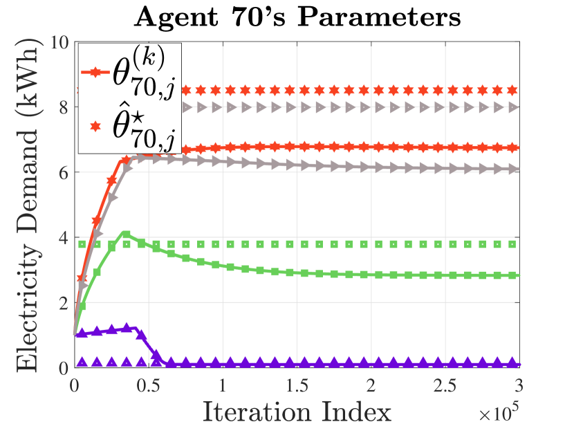
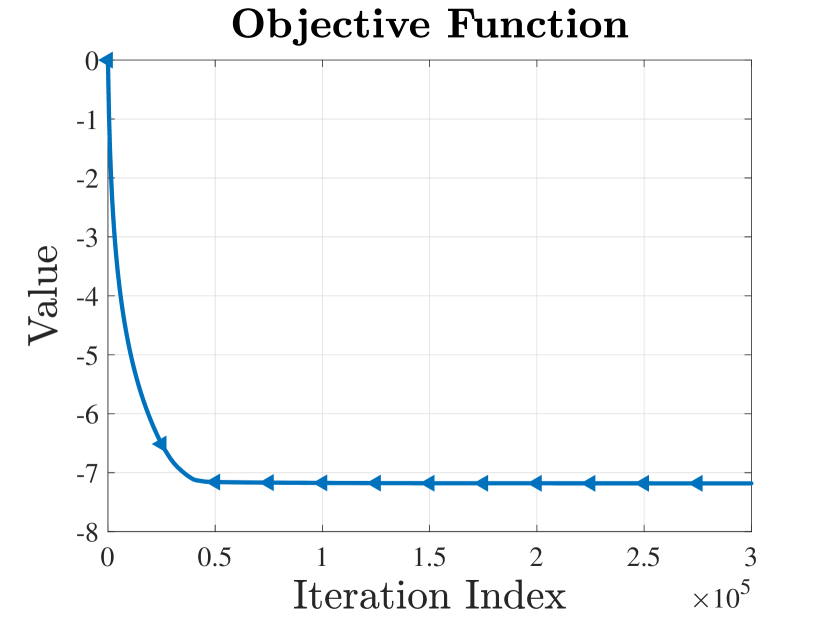
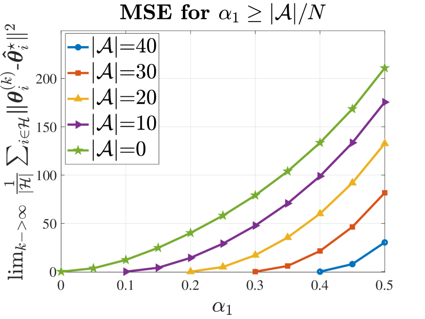
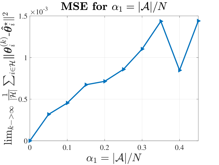
Figure 5: Numerical study results for optimal electric vehicle charging under static impersonation attack. (a) Optimal parameter of agent 70 converges to a neighborhood of the optimal solution of the robust optimization problem for |𝒜|/N=0.2𝒜𝑁0.2|{\cal A}|/N=0.2 and α1=0.3subscript𝛼10.3\alpha_{1}=0.3, (b) The algorithm provides convergence of the objective function value, (c) Mean squared error for different number of compromised channels and different choices of upper bound α1subscript𝛼1\alpha_{1}, (d) Mean squared error when α1=|𝒜|/Nsubscript𝛼1𝒜𝑁\alpha_{1}=|{\cal A}|/N.

V-A1 Static impersonation attack

We simulated various static impersonation attack scenarios and ran Algorithm 2. The results are displayed in Figure 5.

In Figure 5(a), we plot agent 70’s electricity demand for some time periods, with |𝒜|/N=0.2𝒜𝑁0.2|{\cal A}|/N=0.2 and α1=0.3subscript𝛼10.3\alpha_{1}=0.3. Each different color corresponds to a different dimension of the parameter vector (i.e., electricity demand for different time periods). A colored solid line corresponds to a dimension of the parameter vector iterates generated by the algorithm. A dashed line with the same marker and color as a solid line is the optimal value corresponding to that dimension of the parameter vector, which is the solution of the regularized robust optimization problem (formulated as (Pυsubscriptsuperscriptabsent𝜐{}^{\prime}_{\upsilon})) of (34). Observe that Algorithm 2 successfully provides convergence to a close neighborhood of the optimal solution of the regularized robust optimization problem. Furthermore, in Figure 5(b) we show that the objective function value converges, as opposed to a non-resilient PD-DRA method that is shown to oscillate and violate the constraint in Figure 2. Our robust optimization model on the other hand ensures there is no constraint violation.
Refer to caption
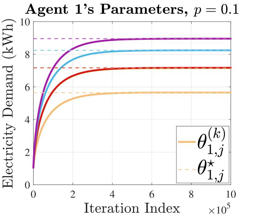
(a) p=0.1𝑝0.1p=0.1, m=20𝑚20m=20, α2=0.45subscript𝛼20.45\alpha_{2}=0.45
Refer to caption
(b) p=0.2𝑝0.2p=0.2, m=100𝑚100m=100, α2=0.49subscript𝛼20.49\alpha_{2}=0.49
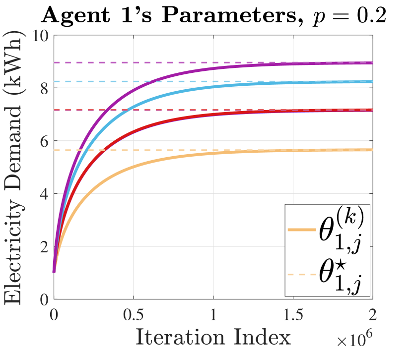
Figure 6: Numerical study results demonstrating convergence of Algorithm 3 for optimal electric vehicle charging under two dynamic impersonation attack scenarios: (a) p=0.1𝑝0.1p=0.1, (b) p=0.2𝑝0.2p=0.2. Observe that the number of iterations it takes to converge for (b) is much larger than for (a).

In Figure 5(c), we plot the mean squared error (MSE) in primal variables 𝜽isubscript𝜽𝑖\bm{\theta}_{i} for different number of compromised channels |𝒜|𝒜|\mathcal{A}| and different choices of α1subscript𝛼1\alpha_{1}, which is the upper bound on fraction of compromised links known by the central coordinator. The MSE is calculated by:

MSE=limk1||i𝜽i(k)𝜽^i2,MSE𝑘1subscript𝑖superscriptnormsuperscriptsubscript𝜽𝑖𝑘subscriptsuperscript^𝜽𝑖2\textnormal{MSE}=\underset{k\rightarrow\infty}{\lim}\frac{1}{|\mathcal{H}|}\sum_{i\in\mathcal{H}}\|\bm{\theta}_{i}^{(k)}-\hat{\bm{\theta}}^{\star}_{i}\|^{2}, (36)

where 𝜽^isubscriptsuperscript^𝜽𝑖\hat{\bm{\theta}}^{\star}_{i} is the solution to (Pυ)italic-(Pυitalic-)\eqref{eq:pdp} with α1=|𝒜|/Nsubscript𝛼1𝒜𝑁\alpha_{1}=|\mathcal{A}|/N, i.e., the solution to the regularized and robustified problem with the knowledge of the compromised channels. Naturally, the looser the upper bound, the larger the error, since it increases the amount of conservatism. Hence, having an accurate upper bound on fraction of compromised channels significantly improves the performance.

Finally, in Figure 5(d) we exhibit the efficacy of our approach with median-based mean estimation. We plot the mean squared error in primal variables, when the upper bound on α1subscript𝛼1\alpha_{1} is tight, i.e., α1=|𝒜|/Nsubscript𝛼1𝒜𝑁\alpha_{1}=|{\cal A}|/N. The error tends to increase with |𝒜|/N𝒜𝑁|{\cal A}|/N, however, considering the magnitude, the error is negligible and we can conclude that the median-based mean estimator performs well.

V-A2 Dynamic impersonation attack

We simulated a dynamic impersonation attack scenario and ran Algorithm 3. To simulate a dynamic impersonation attack, we assigned a probability p𝑝p for an uplink to be compromised at each iteration333Although a probabilistic scenario does not guarantee that Assumption 2 holds, with sufficiently large window size m𝑚m and α2subscript𝛼2\alpha_{2}, it holds with high probability at each iteration. Even though we do not study this scenario theoretically, our algorithm still performs well.. For p=0.1𝑝0.1p=0.1, we picked a window size m=20𝑚20m=20 and α2=0.45subscript𝛼20.45\alpha_{2}=0.45, whereas for p=0.2𝑝0.2p=0.2, we picked a window size m=100𝑚100m=100 and α2=0.49subscript𝛼20.49\alpha_{2}=0.49. The results are displayed in Figure 6. Each different color corresponds to a different dimension of the parameter vector. A colored solid line corresponds to a dimension of the parameter vector iterates generated by the algorithm. A dashed line with the same color as a solid line is the optimal value corresponding to that dimension of the parameter vector, which is the solution of the regularized optimization problem (formulated as (Pυ)) of (34).

In both scenarios, Algorithm 3 successfully provides convergence to the optimal solution of the regularized problem. Observe that for p=0.2𝑝0.2p=0.2, we chose a larger window size and a larger α2subscript𝛼2\alpha_{2} in order to meet Assumption 2. However, this restricts us to choose a smaller step size γ𝛾\gamma as dictated by Theorem 2 and in turn slower convergence. This highlights an important trade-off between robustness and convergence rate, where a larger window size m𝑚m and larger α2subscript𝛼2\alpha_{2} makes the algorithm more robust while decreasing the convergence rate.

V-B Power Distribution Network
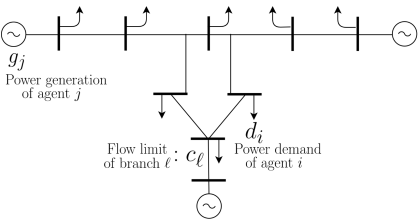
Refer to caption
Figure 7: IEEE 9 bus system with 3 generators (supplies) represented by sources and 8 loads (demands) represented by arrows.

We consider the IEEE N=9𝑁9N=9 bus system with Ng=3subscript𝑁𝑔3N_{g}=3 generators and N=8subscript𝑁8N_{\ell}=8 loads as shown in Figure 7. The power network cost minimization problem can be stated as:

mindi,gi+subscript𝑑𝑖subscript𝑔𝑖superscript\displaystyle\underset{d_{i},g_{i}\in\mathbb{R}^{+}}{\min} f(𝒅,𝒈)=i=1NUi(di)+i=1NgCi(gi)𝑓𝒅𝒈superscriptsubscript𝑖1subscript𝑁subscript𝑈𝑖subscript𝑑𝑖superscriptsubscript𝑖1subscript𝑁𝑔subscript𝐶𝑖subscript𝑔𝑖\displaystyle{\color[rgb]{0,0,0}f}(\bm{d},\bm{g})=-\sum_{i=1}^{N_{\ell}}U_{i}(d_{i})+\sum_{i=1}^{N_{g}}C_{i}(g_{i}) (37a)
subject to 𝟏T(𝒅𝒈)=0,superscript1𝑇𝒅𝒈0\displaystyle\bm{1}^{T}(\bm{d}-\bm{g})=0, (37b)
H(𝒅𝒈)𝒄,H𝒅𝒈𝒄\displaystyle\textnormal{{H}}(\bm{d}-\bm{g})\leq\bm{c}, (37c)

where 𝒅=[d1dN]T𝒅superscriptdelimited-[]subscript𝑑1subscript𝑑𝑁𝑇\bm{d}=[d_{1}\dots d_{N}]^{T} and 𝒈=[g1gN]T𝒈superscriptdelimited-[]subscript𝑔1subscript𝑔𝑁𝑇\bm{g}=[g_{1}\dots g_{N}]^{T} are the vectors of load and generation at each node, respectively (di=0subscript𝑑𝑖0d_{i}=0 for nodes without load and gj=0subscript𝑔𝑗0g_{j}=0 for nodes without generators). The first constraint (37b) ensures the power supply is equal to the demand, and the second constraint (37c) is the power flow constraint limiting the power flow on each branch.
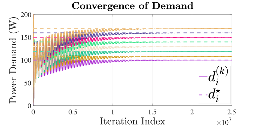
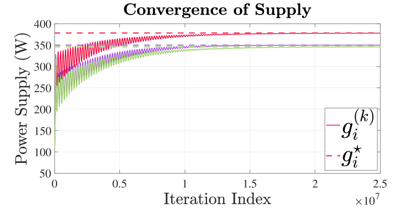
Refer to caption
(a)
Refer to caption
(b)
Figure 8: Numerical study results for power network under dynamic impersonation attack: (a)/(b) displaying convergence of the demand/supply, respectively.

Observe that the formulation in (37) does not directly match with our general formulation in (1) mainly due to the presence of equality constraint (37b), which prevents the application of the robustified formulation in (9) and hence the robust PD-DRA algorithm for static impersonation attacks. Nevertheless, our algorithm for dynamic impersonation attacks can still be applied since it does not require any robustified constraints (which cannot be done for equality constraints).

We have chosen the utility function for load i𝑖i to be Ui(di)=βilogdisubscript𝑈𝑖subscript𝑑𝑖subscript𝛽𝑖subscript𝑑𝑖U_{i}(d_{i})=\beta_{i}\log d_{i} and randomly generated βisubscript𝛽𝑖\beta_{i} from a uniform distribution in [500,1000]5001000[500,1000]. For generators, we set the cost function Ci(gi)=ecigisubscript𝐶𝑖subscript𝑔𝑖superscript𝑒subscript𝑐𝑖subscript𝑔𝑖C_{i}(g_{i})=e^{c_{i}g_{i}}, where c1=0.01,c2=0.011,c3=0.012formulae-sequencesubscript𝑐10.01formulae-sequencesubscript𝑐20.011subscript𝑐30.012c_{1}=0.01,~{}c_{2}=0.011,~{}c_{3}=0.012. We obtained the Power Transfer Distribution Factor (PTDF) matrix H and the vector of flow limits 𝒄𝒄\bm{c} from Matpower[39]. To simulate a dynamic impersonation attack scenario, we assigned a probability p𝑝p for an uplink to be compromised at each iteration. We ran Algorithm 3 for p=0.15𝑝0.15p=0.15, m=75𝑚75m=75 and α2=0.49subscript𝛼20.49\alpha_{2}=0.49.

The results are shown in Figure 8. In both Figures 8(a) and 8(b), each different color corresponds to a different agent. A colored solid line corresponds to an agent’s parameter iterates generated by the algorithm. A dashed line with the same color as a solid line is the to the optimal value of that agent’s parameter, which is the solution of the regularized optimization problem (formulated as (Pυ)) of (37). Our algorithm successfully generates sequences that convergence to the optimal solution of the regularized problem for both power supplying and power demanding agents.

VI Conclusion

In this paper, we studied two strategies for establishing primal-dual algorithms for resource allocation in presence of Byzantine attackers. Specifically, we consider static and dynamic impersonation attack scenarios and propose an attack-resilient primal-dual algorithm for each scenario based on robust mean estimation techniques. We derive bounds for the performance (in terms of distance to optimality) of the proposed algorithms and show that our algorithm for static impersonation attack converges to a neighborhood of the optimal solution of the regularized and robustified resource allocation problem, whereas our algorithm for dynamic impersonation attack converges to the optimal solution of the original regularized problem. We verify our theoretical results via computational simulations for network utility maximization problems involving optimal distributed resource allocation, such as power distribution networks.

References

  • [1] F. P. Kelly, A. K. Maulloo, and D. K. H. Tan, “Rate control for communication networks: shadow prices, proportional fairness and stability,” J OPER RES SOC, vol. 49, no. 3, pp. 237–252, Mar 1998.
  • [2] S. H. Low and D. E. Lapsley, “Optimization flow control. i. basic algorithm and convergence,” IEEE/ACM Transactions on Networking, vol. 7, no. 6, pp. 861–874, Dec 1999.
  • [3] P. Samadi, A. Mohsenian-Rad, R. Schober, V. W. S. Wong, and J. Jatskevich, “Optimal real-time pricing algorithm based on utility maximization for smart grid,” in IEEE SmartGridComm, Oct 2010, pp. 415–420.
  • [4] N. Li, L. Chen, and S. H. Low, “Optimal demand response based on utility maximization in power networks,” in 2011 IEEE Power and Energy Society General Meeting, July 2011, pp. 1–8.
  • [5] M. Chiang and J. Bell, “Balancing supply and demand of bandwidth in wireless cellular networks: utility maximization over powers and rates,” in IEEE INFOCOM 2004, vol. 4, March 2004, pp. 2800–2811 vol.4.
  • [6] M. Dehghan, L. Massoulie, D. Towsley, D. Menasche, and Y. C. Tay, “A utility optimization approach to network cache design,” in IEEE INFOCOM, April 2016, pp. 1–9.
  • [7] M. Zhao, J. Li, and Y. Yang, “Joint mobile energy replenishment and data gathering in wireless rechargeable sensor networks,” in Proceedings of the 23rd International Teletraffic Congress, ser. ITC ’11.   International Teletraffic Congress, 2011, pp. 238–245.
  • [8] R. Deng, Y. Zhang, S. He, J. Chen, and X. Shen, “Maximizing network utility of rechargeable sensor networks with spatiotemporally coupled constraints,” IEEE JSAC, vol. 34, no. 5, pp. 1307–1319, May 2016.
  • [9] N. Mehr, J. Lioris, R. Horowitz, and R. Pedarsani, “Joint perimeter and signal control of urban traffic via network utility maximization,” in IEEE ITSC, Oct 2017, pp. 1–6.
  • [10] J. Koshal, A. Nedić, and U. V. Shanbhag, “Multiuser optimization: Distributed algorithms and error analysis,” SIAM Journal on Optimization, vol. 21, no. 3, pp. 1046–1081, 2011.
  • [11] D. P. Palomar and M. Chiang, “A tutorial on decomposition methods for network utility maximization,” IEEE JSAC, vol. 24, no. 8, pp. 1439–1451, 2006.
  • [12] S. Sundaram and C. N. Hadjicostis, “Distributed function calculation via linear iterative strategies in the presence of malicious agents,” IEEE TAC, vol. 56, no. 7, pp. 1495–1508, 2011.
  • [13] F. Pasqualetti, A. Bicchi, and F. Bullo, “Consensus computation in unreliable networks: A system theoretic approach,” IEEE TAC, vol. 57, no. 1, pp. 90–104, 2012.
  • [14] R. Gentz, S. X. Wu, H.-T. Wai, A. Scaglione, and A. Leshem, “Data injection attacks in randomized gossiping,” IEEE TSIPN, vol. 2, no. 4, pp. 523–538, 2016.
  • [15] S. Sundaram and B. Gharesifard, “Distributed optimization under adversarial nodes,” IEEE TAC, 2018.
  • [16] Y. Chen, S. Kar, and J. Moura, “Resilient distributed estimation: Sensor attacks,” IEEE Transactions on Automatic Control, 2018.
  • [17] W. Ben-Ameur, P. Bianchi, and J. Jakubowicz, “Robust distributed consensus using total variation,” IEEE Transactions on Automatic Control, vol. 61, no. 6, pp. 1550–1564, 2016.
  • [18] H. J. LeBlanc, H. Zhang, X. Koutsoukos, and S. Sundaram, “Resilient asymptotic consensus in robust networks,” IEEE Journal on Selected Areas in Communications, vol. 31, no. 4, pp. 766–781, April 2013.
  • [19] J. S. Baras and X. Liu, “Trust is the cure to distributed consensus with adversaries,” in 2019 27th Mediterranean Conference on Control and Automation (MED), July 2019, pp. 195–202.
  • [20] N. Ravi, A. Scaglione, and A. Nedić, “A case of distributed optimization in adversarial environment,” in 2019 IEEE International Conference on Acoustics, Speech and Signal Processing, May 2019, pp. 5252–5256.
  • [21] J. Feng, H. Xu, and S. Mannor, “Distributed robust learning,” arXiv preprint arXiv:1409.5937, 2014.
  • [22] D. Yin, Y. Chen, K. Ramchandran, and P. Bartlett, “Byzantine-robust distributed learning: Towards optimal statistical rates,” arXiv preprint arXiv:1803.01498, 2018.
  • [23] D. Alistarh, Z. Allen-Zhu, and J. Li, “Byzantine stochastic gradient descent,” in NeurIPS, 2018, pp. 4618–4628.
  • [24] Y. Chen, L. Su, and J. Xu, “Distributed statistical machine learning in adversarial settings: Byzantine gradient descent,” Proc. ACM Meas. Anal. Comput. Syst., vol. 1, no. 2, pp. 44:1–44:25, 2017.
  • [25] D. Data, L. Song, and S. Diggavi, “Data encoding methods for byzantine-resilient distributed optimization,” in 2019 IEEE International Symposium on Information Theory (ISIT), July 2019, pp. 2719–2723.
  • [26] D. L. Donoho and P. J. Huber, “The notion of breakdown point,” A festschrift for Erich L. Lehmann, vol. 157184, 1983.
  • [27] P. J. Huber, Robust statistics.   Springer, 2011.
  • [28] S. Minsker et al., “Geometric median and robust estimation in banach spaces,” Bernoulli, vol. 21, no. 4, pp. 2308–2335, 2015.
  • [29] I. Diakonikolas, G. Kamath, D. M. Kane, J. Li, A. Moitra, and A. Stewart, “Robust estimators in high dimensions without the computational intractability,” in IEEE FOCS, 2016, pp. 655–664.
  • [30] J. Steinhardt, M. Charikar, and G. Valiant, “Resilience: A criterion for learning in the presence of arbitrary outliers,” arXiv preprint arXiv:1703.04940, 2017.
  • [31] C. A. Uribe, H. Wai, and M. Alizadeh, “Resilient distributed optimization algorithms for resource allocation,” in 2019 IEEE 58th Conference on Decision and Control (CDC), 2019, pp. 8341–8346.
  • [32] Y. Nesterov, “Smooth minimization of non-smooth functions,” Mathematical programming, vol. 103, no. 1, pp. 127–152, 2005.
  • [33] C. A. Uribe, S. Lee, A. Gasnikov, and A. Nedić, “A dual approach for optimal algorithms in distributed optimization over networks,” arXiv preprint arXiv:1809.00710, 2018.
  • [34] B. Turan, C. A. Uribe, H.-T. Wai, and M. Alizadeh, “Resilient primal-dual optimization algorithms for distributed resource allocation,” arXiv preprint arXiv:2001.00612, 2020.
  • [35] D. Blatt, A. O. Hero, and H. Gauchman, “A convergent incremental gradient method with a constant step size,” SIAM Journal on Optimization, vol. 18, no. 1, pp. 29–51, 2007.
  • [36] M. Gürbüzbalaban, A. Ozdaglar, and P. A. Parrilo, “On the convergence rate of incremental aggregated gradient algorithms,” SIAM Journal on Optimization, vol. 27, no. 2, pp. 1035–1048, 2017.
  • [37] P. Tseng and S. Yun, “Incrementally updated gradient methods for constrained and regularized optimization,” Journal of Optimization Theory and Applications, vol. 160, no. 3, pp. 832–853, Mar 2014.
  • [38] M. Grant and S. Boyd, “CVX: Matlab software for disciplined convex programming, version 2.1,” http://cvxr.com/cvx, Mar. 2014.
  • [39] R. D. Zimmerman, C. E. Murillo-Sánchez, and R. J. Thomas, “Matpower: Steady-state operations, planning, and analysis tools for power systems research and education,” IEEE Transactions on Power Systems, vol. 26, no. 1, pp. 12–19, Feb 2011.
  • [40] H. R. Feyzmahdavian, A. Aytekin, and M. Johansson, “A delayed proximal gradient method with linear convergence rate,” in 2014 IEEE International Workshop on Machine Learning for Signal Processing (MLSP), Sep. 2014, pp. 1–6.
[Uncaptioned image] BERKAY TURAN is pursuing the Ph.D. degree in Electrical and Computer Engineering at the University of California, Santa Barbara. He received the B.Sc. degree in Electrical and Electronics Engineering as well as the B.Sc. degree in Physics degree from  Boğaziçi University, Istanbul, Turkey, in 2018. His research interests include optimization and reinforcement learning for the design, control, and analysis of smart infrastructure systems such as the power grid and transportation systems.
[Uncaptioned image] CÉSAR A. URIBE received the M.Sc. degrees in systems and control from Delft University of Technology, in The Netherlands, and in applied mathematics from the University of Illinois at Urbana-Champaign, in 2013 and 2016, respectively. He also received the PhD degree in electrical and computer engineering at the University of Illinois at Urbana-Champaign in 2018. He is currently a Postdoctoral Associate in the Laboratory for Information and Decision Systems-LIDS at the Massachusetts Institute of Technology-MIT. His research interests include distributed learning and optimization, decentralized control, algorithm analysis, and computational optimal transport.
[Uncaptioned image] Hoi-To Wai (S’11–M’18) received his PhD degree from Arizona State University (ASU) in Electrical Engineering in Fall 2017, B. Eng. (with First Class Honor) and M. Phil. degrees in Electronic Engineering from The Chinese University of Hong Kong (CUHK) in 2010 and 2012, respectively. He is an Assistant Professor in the Department of Systems Engineering & Engineering Management at CUHK. He has held research positions at ASU, UC Davis, Telecom ParisTech, Ecole Polytechnique, LIDS, MIT. Hoi-To’s research interests are in the broad area of signal processing, machine learning and distributed optimization, with a focus of their applications to network science. His dissertation has received the 2017’s Dean’s Dissertation Award from the Ira A. Fulton Schools of Engineering of ASU and he is a recipient of a Best Student Paper Award at ICASSP 2018.
[Uncaptioned image] MAHNOOSH ALIZADEH is an assistant professor of Electrical and Computer Engineering at the University of California Santa Barbara. She received the B.Sc. degree (’09) in Electrical Engineering from Sharif University of Technology and the M.Sc. (’13) and Ph.D. (’14) degrees in Electrical and Computer Engineering from the University of California Davis, where she was the recipient of the Richard C. Dorf award for outstanding research accomplishment. From 2014 to 2016, she was a postdoctoral scholar at Stanford University. Her research interests are focused on designing network control, optimization, and learning frameworks to promote efficiency and resiliency in societal-scale cyber-physical systems. Dr. Alizadeh is a recipient of the NSF CAREER award and the best paper award from HICSS-53 power systems track.

-A Proof of Lemma 1

Observe that in both (9) and (12), the decision variables of the optimization problems are {𝜽i}isubscriptsubscript𝜽𝑖𝑖\{\bm{\theta}_{i}\}_{i\in{\cal H}}. Hence, it suffices to show that any given set of {𝜽i}isubscriptsubscript𝜽𝑖𝑖\{\bm{\theta}_{i}\}_{i\in{\cal H}} satisfying constraints of (12) also satisfies constraints of (9). Let 𝜽¯𝒜:=1|𝒜|i𝒜𝜽iassignsubscript¯𝜽𝒜1𝒜subscript𝑖𝒜subscript𝜽𝑖\overline{\bm{\theta}}_{\mathcal{A}}\vcentcolon=\frac{1}{|\mathcal{A}|}\sum_{i\in\mathcal{A}}\bm{\theta}_{i}. Since gtsubscript𝑔𝑡g_{t} is L𝐿L-smooth, the following holds:

max𝜽j𝒞j,j𝒜gt(1Ni=1N𝜽i)=max𝜽j𝒞j,j𝒜gt(||N𝜽¯+|𝒜|N𝜽¯𝒜)=max𝜽j𝒞j,j𝒜gt((1α1)𝜽¯+(α1|𝒜|N)𝜽¯+|𝒜|N𝜽¯𝒜)max𝜽j𝒞j,j𝒜(gt((1α1)𝜽¯)+𝜽~,gt((1α1)𝜽¯)+L2𝜽~2),formulae-sequencesubscript𝜽𝑗subscript𝒞𝑗𝑗𝒜subscript𝑔𝑡1𝑁superscriptsubscript𝑖1𝑁subscript𝜽𝑖formulae-sequencesubscript𝜽𝑗subscript𝒞𝑗𝑗𝒜subscript𝑔𝑡𝑁subscript¯𝜽𝒜𝑁subscript¯𝜽𝒜formulae-sequencesubscript𝜽𝑗subscript𝒞𝑗𝑗𝒜subscript𝑔𝑡1subscript𝛼1subscript¯𝜽subscript𝛼1𝒜𝑁subscript¯𝜽𝒜𝑁subscript¯𝜽𝒜formulae-sequencesubscript𝜽𝑗subscript𝒞𝑗𝑗𝒜subscript𝑔𝑡1subscript𝛼1subscript¯𝜽~𝜽subscript𝑔𝑡1subscript𝛼1subscript¯𝜽𝐿2superscriptdelimited-∥∥~𝜽2\begin{split}&\underset{\bm{\theta}_{j}\in\mathcal{C}_{j},j\in\mathcal{A}}{\max}\textstyle g_{t}\big{(}\frac{1}{N}\sum_{i=1}^{N}\bm{\theta}_{i}\big{)}=\underset{\bm{\theta}_{j}\in\mathcal{C}_{j},j\in\mathcal{A}}{\max}g_{t}\big{(}\frac{|\mathcal{H}|}{N}\overline{\bm{\theta}}_{\mathcal{H}}+\frac{|\mathcal{A}|}{N}\overline{\bm{\theta}}_{\mathcal{A}})\\ &\textstyle=\underset{\bm{\theta}_{j}\in\mathcal{C}_{j},j\in\mathcal{A}}{\max}g_{t}\big{(}(1-\alpha_{1})\overline{\bm{\theta}}_{\mathcal{H}}+(\alpha_{1}-\frac{|\mathcal{A}|}{N})\overline{\bm{\theta}}_{\mathcal{H}}+\frac{|\mathcal{A}|}{N}\overline{\bm{\theta}}_{\mathcal{A}}\big{)}\\ &\textstyle\leq\underset{\bm{\theta}_{j}\in\mathcal{C}_{j},j\in\mathcal{A}}{\max}\bigg{(}g_{t}\big{(}(1-\alpha_{1})\overline{\bm{\theta}}_{\mathcal{H}}\big{)}\\ &\hskip 56.9055pt+\Big{\langle}\widetilde{\bm{\theta}},\nabla g_{t}\big{(}(1-\alpha_{1})\overline{\bm{\theta}}_{\mathcal{H}}\big{)}\Big{\rangle}+\frac{L}{2}\|\widetilde{\bm{\theta}}\|^{2}\bigg{)},\end{split} (38)

where we defined 𝜽~:=(α1|𝒜|N)𝜽¯+|𝒜|N𝜽¯𝒜assign~𝜽subscript𝛼1𝒜𝑁subscript¯𝜽𝒜𝑁subscript¯𝜽𝒜\widetilde{\bm{\theta}}\vcentcolon=(\alpha_{1}-\frac{|\mathcal{A}|}{N})\overline{\bm{\theta}}_{\mathcal{H}}+\frac{|\mathcal{A}|}{N}\overline{\bm{\theta}}_{\mathcal{A}}. Observe that

𝜽~(α1|𝒜|N)𝜽¯+|𝒜|N𝜽¯𝒜α1R.norm~𝜽subscript𝛼1𝒜𝑁normsubscript¯𝜽𝒜𝑁normsubscript¯𝜽𝒜subscript𝛼1𝑅\textstyle\|\widetilde{\bm{\theta}}\|\leq(\alpha_{1}-\frac{|\mathcal{A}|}{N})\|\overline{\bm{\theta}}_{\mathcal{H}}\|+\frac{|\mathcal{A}|}{N}\|\overline{\bm{\theta}}_{\mathcal{A}}\|\leq\alpha_{1}R. (39)

Furthermore, since the gradient of gtsubscript𝑔𝑡g_{t} is uniformly bounded by B𝐵B and α12α1superscriptsubscript𝛼12subscript𝛼1\alpha_{1}^{2}\leq\alpha_{1}, (LABEL:eq:robustconstraintproof) can be upper bounded by:

gt((1α1)𝜽¯)+α1(RB+12LR2)subscript𝑔𝑡1subscript𝛼1subscript¯𝜽subscript𝛼1𝑅𝐵12𝐿superscript𝑅2g_{t}\big{(}(1-\alpha_{1})\overline{\bm{\theta}}_{\mathcal{H}}\big{)}+\alpha_{1}\big{(}RB+{\textstyle\frac{1}{2}}LR^{2}\big{)} (40)

Hence, we have shown that for any given set of {𝜽i}isubscriptsubscript𝜽𝑖𝑖\{\bm{\theta}_{i}\}_{i\in{\cal H}}, the following holds:

max𝜽j𝒞j,j𝒜gt(1Ni=1N𝜽i)gt((1α1)𝜽¯)+α1(RB+12LR2).formulae-sequencesubscript𝜽𝑗subscript𝒞𝑗𝑗𝒜subscript𝑔𝑡1𝑁superscriptsubscript𝑖1𝑁subscript𝜽𝑖subscript𝑔𝑡1subscript𝛼1subscript¯𝜽subscript𝛼1𝑅𝐵12𝐿superscript𝑅2\underset{\bm{\theta}_{j}\in\mathcal{C}_{j},j\in\mathcal{A}}{\max}g_{t}\big{(}{\textstyle\frac{1}{N}\sum_{i=1}^{N}\bm{\theta}_{i}}\big{)}\leq g_{t}\big{(}(1-\alpha_{1})\overline{\bm{\theta}}_{\mathcal{H}}\big{)}+\alpha_{1}\big{(}RB+{\textstyle\frac{1}{2}}LR^{2}\big{)}. (41)

As such defining ct:=α1(RB+12LR2)assignsubscript𝑐𝑡subscript𝛼1𝑅𝐵12𝐿superscript𝑅2c_{t}\vcentcolon=\alpha_{1}\big{(}RB+\frac{1}{2}LR^{2}\big{)}, it can be seen that if a set of {𝜽i}isubscriptsubscript𝜽𝑖𝑖\{\bm{\theta}_{i}\}_{i\in{\cal H}} satisfies

gt((1α1)𝜽¯)+ct0,t=1,,T,formulae-sequencesubscript𝑔𝑡1subscript𝛼1subscript¯𝜽subscript𝑐𝑡0𝑡1𝑇g_{t}\big{(}(1-\alpha_{1})\overline{\bm{\theta}}_{\mathcal{H}}\big{)}+c_{t}\leq 0,~{}t=1,...,T, (42)

the same set of {𝜽i}isubscriptsubscript𝜽𝑖𝑖\{\bm{\theta}_{i}\}_{i\in{\cal H}} satisfies the desired constraint (9).

-B Proof of Proposition 2

Fix any j[d]𝑗delimited-[]𝑑j\in[d]. The assumption implies that for all i𝑖i\in{\cal H}, one has:

|[𝒙i𝒙¯]j|r.subscriptdelimited-[]subscript𝒙𝑖subscript¯𝒙𝑗𝑟|[\bm{x}_{i}-\overline{\bm{x}}_{\cal H}]_{j}|\leq r. (43)

We observe that ||(1α1)N1subscript𝛼1𝑁|{\cal H}|\geq(1-\alpha_{1})N. Applying [21, Lemma 1] shows that the median estimator444At each coordinate, the median is the geometric median estimator of one dimension in [21]. satisfies

|[𝒙𝗆𝖾𝖽𝒙¯]j|(1α1)112α1r.subscriptdelimited-[]subscript𝒙𝗆𝖾𝖽subscript¯𝒙𝑗1subscript𝛼1112subscript𝛼1𝑟|[{\bm{x}}_{\sf med}-\overline{\bm{x}}_{\cal H}]_{j}|\leq(1-\alpha_{1})\sqrt{\frac{1}{1-2\alpha_{1}}}r. (44)

The above implies that for all i𝑖i\in{\cal H}, we have

|[𝒙i𝒙𝗆𝖾𝖽]j|(1+(1α1)212α1)r.subscriptdelimited-[]subscript𝒙𝑖subscript𝒙𝗆𝖾𝖽𝑗1superscript1subscript𝛼1212subscript𝛼1𝑟|[\bm{x}_{i}-{\bm{x}}_{\sf med}]_{j}|\leq\left(1+\sqrt{\frac{(1-\alpha_{1})^{2}}{1-2\alpha_{1}}}\right)r. (45)

This implies that rj(1+(1α1)212α1)rsubscript𝑟𝑗1superscript1subscript𝛼1212subscript𝛼1𝑟r_{j}\leq\left(1+\sqrt{\frac{(1-\alpha_{1})^{2}}{1-2\alpha_{1}}}\right)r, since ||(1α1)N1subscript𝛼1𝑁|{\cal H}|\geq(1-\alpha_{1})N. We then bound the performance of 𝒙^subscript^𝒙\widehat{\bm{x}}_{\mathcal{H}}:

(1α1)N[𝒙^]j=i𝒩j[𝒙i]j=i[𝒙i]ji𝒩j[𝒙i]j+i𝒜𝒩j[𝒙i]j,1subscript𝛼1𝑁subscriptdelimited-[]subscript^𝒙𝑗subscript𝑖subscript𝒩𝑗subscriptdelimited-[]subscript𝒙𝑖𝑗subscript𝑖subscriptdelimited-[]subscript𝒙𝑖𝑗subscript𝑖subscript𝒩𝑗subscriptdelimited-[]subscript𝒙𝑖𝑗subscript𝑖𝒜subscript𝒩𝑗subscriptdelimited-[]subscript𝒙𝑖𝑗\begin{split}&(1-\alpha_{1})N[\widehat{\bm{x}}_{\mathcal{H}}]_{j}=\sum_{i\in{\cal N}_{j}}[{\bm{x}}_{i}]_{j}\\ &=\sum_{i\in{\cal H}}[{\bm{x}}_{i}]_{j}-\sum_{i\in{\cal H}\setminus{\cal N}_{j}}[{\bm{x}}_{i}]_{j}+\sum_{i\in{\cal A}\cap{\cal N}_{j}}[{\bm{x}}_{i}]_{j},\end{split} (46)

thus

(1α1)N[𝒙^𝒙¯]j=i𝒩j[𝒙i𝒙¯]j+i𝒜𝒩j[𝒙i𝒙¯]j=i𝒩j[𝒙i𝒙¯]j+i𝒜𝒩j[𝒙i𝒙𝗆𝖾𝖽+𝒙𝗆𝖾𝖽𝒙¯]j1subscript𝛼1𝑁subscriptdelimited-[]subscript^𝒙subscript¯𝒙𝑗subscript𝑖subscript𝒩𝑗subscriptdelimited-[]subscript𝒙𝑖subscript¯𝒙𝑗subscript𝑖𝒜subscript𝒩𝑗subscriptdelimited-[]subscript𝒙𝑖subscript¯𝒙𝑗subscript𝑖subscript𝒩𝑗subscriptdelimited-[]subscript𝒙𝑖subscript¯𝒙𝑗subscript𝑖𝒜subscript𝒩𝑗subscriptdelimited-[]subscript𝒙𝑖subscript𝒙𝗆𝖾𝖽subscript𝒙𝗆𝖾𝖽subscript¯𝒙𝑗\begin{split}&(1-\alpha_{1})N[\widehat{\bm{x}}_{\cal H}-\overline{\bm{x}}_{\cal H}]_{j}\\ &=-\sum_{i\in{\cal H}\setminus{\cal N}_{j}}[{\bm{x}}_{i}-\overline{\bm{x}}_{\cal H}]_{j}+\sum_{i\in{\cal A}\cap{\cal N}_{j}}[{\bm{x}}_{i}-\overline{\bm{x}}_{\cal H}]_{j}\\ &=-\sum_{i\in{\cal H}\setminus{\cal N}_{j}}[{\bm{x}}_{i}-\overline{\bm{x}}_{\cal H}]_{j}+\sum_{i\in{\cal A}\cap{\cal N}_{j}}[{\bm{x}}_{i}-{\bm{x}}_{\sf med}+{\bm{x}}_{\sf med}-\overline{\bm{x}}_{\cal H}]_{j}\end{split} (47)

Notice that |𝒜𝒩j|α1N𝒜subscript𝒩𝑗subscript𝛼1𝑁|{\cal A}\cap{\cal N}_{j}|\leq\alpha_{1}N and thus |𝒩j|α1Nsubscript𝒩𝑗subscript𝛼1𝑁|{\cal H}\setminus{\cal N}_{j}|\leq\alpha_{1}N. Gathering terms shows

|[𝒙^𝒙¯]j|2α1N(1α1)N(1+(1α1)212α1)r.subscriptdelimited-[]^𝒙subscript¯𝒙𝑗2subscript𝛼1𝑁1subscript𝛼1𝑁1superscript1subscript𝛼1212subscript𝛼1𝑟|[\widehat{\bm{x}}-\overline{\bm{x}}_{\cal H}]_{j}|\leq\frac{2\alpha_{1}N}{(1-\alpha_{1})N}\left(1+\sqrt{\frac{(1-\alpha_{1})^{2}}{1-2\alpha_{1}}}\right)r. (48)

The above holds for all j[d]𝑗delimited-[]𝑑j\in[d]. Applying the norm equivalence shows the desired bound.

-C Proof of Lemma 2

Let [𝒆𝜽(k)]isubscriptdelimited-[]superscriptsubscript𝒆𝜽𝑘𝑖\big{[}{\bm{e}}_{\bm{\theta}}^{(k)}\big{]}_{i} denote the i𝑖ith block of 𝒆𝜽(k)superscriptsubscript𝒆𝜽𝑘{\bm{e}}_{\bm{\theta}}^{(k)}, and [𝒈^𝜽(k)]isubscriptdelimited-[]superscriptsubscript^𝒈𝜽𝑘𝑖\big{[}\widehat{\bm{g}}_{\bm{\theta}}^{(k)}\big{]}_{i} denote the i𝑖ith block of 𝒈^𝜽(k)superscriptsubscript^𝒈𝜽𝑘\widehat{\bm{g}}_{\bm{\theta}}^{(k)}. From Equation (18a):

[𝒈^𝜽(k)]i=1N(𝒈^(k)+𝜽ifi(𝜽i(k))+υ𝜽i(k)).subscriptdelimited-[]superscriptsubscript^𝒈𝜽𝑘𝑖1𝑁subscriptsuperscript^𝒈𝑘subscriptsubscript𝜽𝑖subscript𝑓𝑖superscriptsubscript𝜽𝑖𝑘𝜐superscriptsubscript𝜽𝑖𝑘\big{[}\widehat{\bm{g}}_{\bm{\theta}}^{(k)}\big{]}_{i}=\frac{1}{N}\big{(}\widehat{\bm{g}}^{(k)}_{\cal H}+\nabla_{\bm{\theta}_{i}}f_{i}(\bm{\theta}_{i}^{(k)})+\upsilon\bm{\theta}_{i}^{(k)}\big{)}. (49)

Furthermore, we replace 𝒈^(k)subscriptsuperscript^𝒈𝑘\widehat{\bm{g}}^{(k)}_{\cal H} from Algorithm 2 Step 3(c):

[𝒈^𝜽(k)]i=1N(t=1Tλt(k)𝜽g¯t((1α1)𝜽^(k))+𝜽ifi(𝜽i(k))+υ𝜽i(k)).subscriptdelimited-[]superscriptsubscript^𝒈𝜽𝑘𝑖1𝑁superscriptsubscript𝑡1𝑇superscriptsubscript𝜆𝑡𝑘subscript𝜽subscript¯𝑔𝑡1subscript𝛼1superscriptsubscript^𝜽𝑘subscriptsubscript𝜽𝑖subscript𝑓𝑖superscriptsubscript𝜽𝑖𝑘𝜐superscriptsubscript𝜽𝑖𝑘\big{[}\widehat{\bm{g}}_{\bm{\theta}}^{(k)}\big{]}_{i}=\frac{1}{N}\Big{(}\sum_{t=1}^{T}\lambda_{t}^{(k)}\nabla_{\bm{\theta}}\overline{g}_{t}((1-\alpha_{1})\widehat{\bm{\theta}}_{\cal H}^{(k)})+\nabla_{\bm{\theta}_{i}}f_{i}(\bm{\theta}_{i}^{(k)})+\upsilon\bm{\theta}_{i}^{(k)}\Big{)}. (50)

The perturbation [𝒆𝜽(k)]i=[𝒈^𝜽(k)]i𝜽i¯υ({𝜽i}i;𝝀;)subscriptdelimited-[]superscriptsubscript𝒆𝜽𝑘𝑖subscriptdelimited-[]superscriptsubscript^𝒈𝜽𝑘𝑖subscriptsubscript𝜽𝑖subscript¯𝜐subscriptsubscript𝜽𝑖𝑖𝝀\big{[}{\bm{e}}_{\bm{\theta}}^{(k)}\big{]}_{i}=\big{[}\widehat{\bm{g}}_{\bm{\theta}}^{(k)}\big{]}_{i}-\nabla_{\bm{\theta}_{i}}\overline{\cal L}_{\upsilon}(\{\bm{\theta}_{i}\}_{i\in{\cal H}};\bm{\lambda};{\cal H}) is given by the difference between (50) and (14a):

[𝒆𝜽(k)]i=1Nt=1Tλt(k)(𝜽g¯t((1α1)𝜽^(k))(1α1)N||𝜽g¯t((1α1)𝜽¯(k))).subscriptdelimited-[]superscriptsubscript𝒆𝜽𝑘𝑖1𝑁superscriptsubscript𝑡1𝑇superscriptsubscript𝜆𝑡𝑘subscript𝜽subscript¯𝑔𝑡1subscript𝛼1superscriptsubscript^𝜽𝑘1subscript𝛼1𝑁subscript𝜽subscript¯𝑔𝑡1subscript𝛼1subscriptsuperscript¯𝜽𝑘\begin{split}\big{[}{\bm{e}}_{\bm{\theta}}^{(k)}\big{]}_{i}=\frac{1}{N}\sum_{t=1}^{T}&\lambda_{t}^{(k)}\Big{(}\nabla_{\bm{\theta}}\overline{g}_{t}((1-\alpha_{1})\widehat{\bm{\theta}}_{\cal H}^{(k)})\\ &-\frac{(1-\alpha_{1})N}{|\mathcal{H}|}\nabla_{\bm{\theta}}\overline{g}_{t}((1-\alpha_{1})\bar{\bm{\theta}}^{(k)}_{\mathcal{H}})\Big{)}.\end{split} (51)

By adding and subtracting 1N(t=1Tλt(k)𝜽g¯t((1α1)𝜽¯(k))\frac{1}{N}\Big{(}\sum_{t=1}^{T}\lambda_{t}^{(k)}\nabla_{\bm{\theta}}\overline{g}_{t}((1-\alpha_{1})\bar{\bm{\theta}}^{(k)}_{\mathcal{H}}\Big{)}, the above expression becomes:

[𝒆𝜽(k)]i=1Nt=1Tλt(k)(\displaystyle\big{[}{\bm{e}}_{\bm{\theta}}^{(k)}\big{]}_{i}=\frac{1}{N}{\sum_{t=1}^{T}}\lambda_{t}^{(k)}\Big{(} 𝜽g¯t((1α1)𝜽^(k))subscript𝜽subscript¯𝑔𝑡1subscript𝛼1superscriptsubscript^𝜽𝑘\displaystyle\nabla_{\bm{\theta}}\overline{g}_{t}\big{(}{\textstyle(1-\alpha_{1})}\widehat{\bm{\theta}}_{\cal H}^{(k)}\big{)} (52)
𝜽g¯t((1α1)𝜽¯(k))subscript𝜽subscript¯𝑔𝑡1subscript𝛼1superscriptsubscript¯𝜽𝑘\displaystyle-\nabla_{\bm{\theta}}\overline{g}_{t}\big{(}{\textstyle(1-\alpha_{1})}\overline{\bm{\theta}}_{\cal H}^{(k)}\big{)}
+||(1α1)N||𝜽g¯t((1α1)𝜽¯(k)))\displaystyle+\frac{|\mathcal{H}|-(1-\alpha_{1})N}{|\mathcal{H}|}\nabla_{\bm{\theta}}\overline{g}_{t}\big{(}{\textstyle(1-\alpha_{1})}\overline{\bm{\theta}}_{\cal H}^{(k)}\big{)}\Big{)}

Similarly, comparing (19b) with (18b) and (14b), we identify that:

[𝒆𝝀(k)]t=g¯t((1α1)𝜽^(k))g¯t((1α1)𝜽¯(k)).subscriptdelimited-[]superscriptsubscript𝒆𝝀𝑘𝑡subscript¯𝑔𝑡1subscript𝛼1superscriptsubscript^𝜽𝑘subscript¯𝑔𝑡1subscript𝛼1superscriptsubscript¯𝜽𝑘\big{[}{\bm{e}}_{\bm{\lambda}}^{(k)}\big{]}_{t}=\overline{g}_{t}\big{(}{\textstyle(1-\alpha_{1})}\widehat{\bm{\theta}}_{\cal H}^{(k)}\big{)}-\overline{g}_{t}\big{(}{\textstyle(1-\alpha_{1})}\overline{\bm{\theta}}_{\cal H}^{(k)}\big{)}. (53)

Using Assumption 1 and the said assumptions, we immediately see that

[𝒆𝜽(k)]inormsubscriptdelimited-[]superscriptsubscript𝒆𝜽𝑘𝑖absent\displaystyle\|\big{[}{\bm{e}}_{\bm{\theta}}^{(k)}\big{]}_{i}\|\leq (1α1)λ¯LTN𝜽^(k)𝜽¯(k)1subscript𝛼1¯𝜆𝐿𝑇𝑁normsuperscriptsubscript^𝜽𝑘superscriptsubscript¯𝜽𝑘\displaystyle(1-\alpha_{1})\frac{\overline{\lambda}LT}{N}\|\widehat{\bm{\theta}}_{\cal H}^{(k)}-\overline{\bm{\theta}}_{\cal H}^{(k)}\| (54)
+||(1α1)N||λ¯BTN1subscript𝛼1𝑁¯𝜆𝐵𝑇𝑁\displaystyle+\frac{|\mathcal{H}|-(1-\alpha_{1})N}{|\mathcal{H}|}\frac{\overline{\lambda}BT}{N}

which then implies (20). Assumption 1 implies that g¯tsubscript¯𝑔𝑡\overline{g}_{t} is B𝐵B-Lipschitz continuous, therefore

|[𝒆𝝀(k)]t|B(1α1)𝜽^(k)𝜽¯(k),subscriptdelimited-[]superscriptsubscript𝒆𝝀𝑘𝑡𝐵1subscript𝛼1normsuperscriptsubscript^𝜽𝑘superscriptsubscript¯𝜽𝑘|\big{[}{\bm{e}}_{\bm{\lambda}}^{(k)}\big{]}_{t}|\leq B(1-\alpha_{1})\|\widehat{\bm{\theta}}_{\cal H}^{(k)}-\overline{\bm{\theta}}_{\cal H}^{(k)}\|, (55)

which implies (21).

-D Proof of Theorem 1

Based on Lemma 2, our idea is to perform a perturbation analysis on the PDA algorithm. Without loss of generality, we assume N=1𝑁1N=1 and denote 𝜽=𝜽1𝜽subscript𝜽1\bm{\theta}=\bm{\theta}_{1}. To simplify notations we define υ:=(1α1)υassignsuperscript𝜐1subscript𝛼1𝜐\upsilon^{\prime}\vcentcolon=(1-\alpha_{1})\upsilon. We also drop the subscript, denote the modified and regularized Lagrangian function as =¯υsubscript¯𝜐{\cal L}=\overline{\cal L}_{\upsilon}. Furthermore, we denote the saddle point to (Pυsubscriptsuperscriptabsent𝜐{}^{\prime}_{\upsilon}) as 𝒛=(𝜽,𝝀)superscript𝒛superscript𝜽superscript𝝀{\bm{z}}^{\star}=(\bm{\theta}^{\star},\bm{\lambda}^{\star}).

Using the fact that 𝜽=𝒫𝒞(𝜽)=𝒫𝒞(𝜽γ𝜽(𝜽,𝝀))superscript𝜽subscript𝒫𝒞superscript𝜽subscript𝒫𝒞superscript𝜽𝛾subscript𝜽superscript𝜽superscript𝝀\bm{\theta}^{\star}={\cal P}_{\mathcal{C}}(\bm{\theta}^{\star})={\cal P}_{\mathcal{C}}\big{(}\bm{\theta}^{\star}-\gamma\nabla_{\bm{\theta}}{\cal L}(\bm{\theta}^{\star},\bm{\lambda}^{\star})\big{)}, we observe that in the primal update:

𝜽(k+1)𝜽2superscriptnormsuperscript𝜽𝑘1superscript𝜽2\displaystyle\|\bm{\theta}^{(k+1)}-\bm{\theta}^{\star}\|^{2}
(a)𝜽(k)𝜽22γ𝒈^𝜽(k)𝜽(𝜽,𝝀),𝜽(k)𝜽𝑎superscriptnormsuperscript𝜽𝑘superscript𝜽22𝛾superscriptsubscript^𝒈𝜽𝑘subscript𝜽superscript𝜽superscript𝝀superscript𝜽𝑘superscript𝜽\displaystyle\overset{(a)}{\leq}\|\bm{\theta}^{(k)}-\bm{\theta}^{\star}\|^{2}-2\gamma\langle\widehat{\bm{g}}_{\bm{\theta}}^{(k)}-\nabla_{\bm{\theta}}{\cal L}(\bm{\theta}^{\star},\bm{\lambda}^{\star}),\bm{\theta}^{(k)}-\bm{\theta}^{\star}\rangle
+γ2𝒈^𝜽(k)𝜽(𝜽,𝝀)2superscript𝛾2superscriptnormsuperscriptsubscript^𝒈𝜽𝑘subscript𝜽superscript𝜽superscript𝝀2\displaystyle\hskip 22.76228pt+\gamma^{2}\|\widehat{\bm{g}}_{\bm{\theta}}^{(k)}-\nabla_{\bm{\theta}}{\cal L}(\bm{\theta}^{\star},\bm{\lambda}^{\star})\|^{2} (56)

where (a) is due to the projection inequality 𝒫𝒞(𝒙𝒚)𝒙𝒚normsubscript𝒫𝒞𝒙𝒚norm𝒙𝒚\|{\cal P}_{\mathcal{C}}({\bm{x}}-{\bm{y}})\|\leq\|{\bm{x}}-{\bm{y}}\|. Furthermore, using the Young’s inequality, for any c0,c1>0subscript𝑐0subscript𝑐10c_{0},c_{1}>0, we have

𝜽(k+1)𝜽2superscriptnormsuperscript𝜽𝑘1superscript𝜽2\displaystyle\|\bm{\theta}^{(k+1)}-\bm{\theta}^{\star}\|^{2}
𝜽(k)𝜽2absentsuperscriptnormsuperscript𝜽𝑘superscript𝜽2\displaystyle\leq\|\bm{\theta}^{(k)}-\bm{\theta}^{\star}\|^{2}
2γ𝜽(𝜽(k),𝝀(k))𝜽(𝜽,𝝀),𝜽(k)𝜽2𝛾subscript𝜽superscript𝜽𝑘superscript𝝀𝑘subscript𝜽superscript𝜽superscript𝝀superscript𝜽𝑘superscript𝜽\displaystyle\hskip 14.22636pt-2\gamma\langle\nabla_{\bm{\theta}}{\cal L}(\bm{\theta}^{(k)},\bm{\lambda}^{(k)})-\nabla_{\bm{\theta}}{\cal L}(\bm{\theta}^{\star},\bm{\lambda}^{\star}),\bm{\theta}^{(k)}-\bm{\theta}^{\star}\rangle
+γ2(1+c0)𝜽(𝜽(k),𝝀(k))𝜽(𝜽,𝝀)2superscript𝛾21subscript𝑐0superscriptnormsubscript𝜽superscript𝜽𝑘superscript𝝀𝑘subscript𝜽superscript𝜽superscript𝝀2\displaystyle\hskip 14.22636pt{+\gamma^{2}(1+c_{0})\|\nabla_{\bm{\theta}}{\cal L}(\bm{\theta}^{(k)},\bm{\lambda}^{(k)})-\nabla_{\bm{\theta}}{\cal L}(\bm{\theta}^{\star},\bm{\lambda}^{\star})\|^{2}}
2γ𝒆𝜽(k),𝜽(k)𝜽+γ2(1+1c0)𝒆𝜽(k)22𝛾superscriptsubscript𝒆𝜽𝑘superscript𝜽𝑘superscript𝜽superscript𝛾211subscript𝑐0superscriptnormsuperscriptsubscript𝒆𝜽𝑘2\displaystyle\hskip 14.22636pt{-2\gamma\langle{\bm{e}}_{\bm{\theta}}^{(k)},\bm{\theta}^{(k)}-\bm{\theta}^{\star}\rangle+\gamma^{2}\big{(}1+\frac{1}{c_{0}}\big{)}\|{\bm{e}}_{\bm{\theta}}^{(k)}\|^{2}}
(1+2c1γ)𝜽(k)𝜽2absent12subscript𝑐1𝛾superscriptnormsuperscript𝜽𝑘superscript𝜽2\displaystyle\leq(1+2c_{1}\gamma)\!~{}\|\bm{\theta}^{(k)}-\bm{\theta}^{\star}\|^{2}
2γ𝜽(𝜽(k),𝝀(k))𝜽(𝜽,𝝀),𝜽(k)𝜽2𝛾subscript𝜽superscript𝜽𝑘superscript𝝀𝑘subscript𝜽superscript𝜽superscript𝝀superscript𝜽𝑘superscript𝜽\displaystyle\hskip 14.22636pt-2\gamma\langle\nabla_{\bm{\theta}}{\cal L}(\bm{\theta}^{(k)},\bm{\lambda}^{(k)})-\nabla_{\bm{\theta}}{\cal L}(\bm{\theta}^{\star},\bm{\lambda}^{\star}),\bm{\theta}^{(k)}-\bm{\theta}^{\star}\rangle
+γ2(1+c0)𝜽(𝜽(k),𝝀(k))𝜽(𝜽,𝝀)2superscript𝛾21subscript𝑐0superscriptnormsubscript𝜽superscript𝜽𝑘superscript𝝀𝑘subscript𝜽superscript𝜽superscript𝝀2\displaystyle\hskip 14.22636pt+\gamma^{2}(1+c_{0})\|\nabla_{\bm{\theta}}{\cal L}(\bm{\theta}^{(k)},\bm{\lambda}^{(k)})-\nabla_{\bm{\theta}}{\cal L}(\bm{\theta}^{\star},\bm{\lambda}^{\star})\|^{2}
+(2γc1+γ2+γ2c0)𝒆𝜽(k)2.2𝛾subscript𝑐1superscript𝛾2superscript𝛾2subscript𝑐0superscriptnormsuperscriptsubscript𝒆𝜽𝑘2\displaystyle\hskip 14.22636pt+\Big{(}\frac{2\gamma}{c_{1}}+\gamma^{2}+\frac{\gamma^{2}}{c_{0}}\Big{)}\|{\bm{e}}_{\bm{\theta}}^{(k)}\|^{2}. (57)

Similarly, in the dual update we get,

𝝀(k+1)𝝀2superscriptnormsuperscript𝝀𝑘1superscript𝝀2\displaystyle\|\bm{\lambda}^{(k+1)}-\bm{\lambda}^{\star}\|^{2}
𝝀(k)𝝀2+γ2𝒈^𝝀(k)𝝀(𝜽,𝝀)2absentsuperscriptnormsuperscript𝝀𝑘superscript𝝀2superscript𝛾2superscriptnormsuperscriptsubscript^𝒈𝝀𝑘subscript𝝀superscript𝜽superscript𝝀2\displaystyle\leq\|\bm{\lambda}^{(k)}-\bm{\lambda}^{\star}\|^{2}+\gamma^{2}\|\widehat{\bm{g}}_{\bm{\lambda}}^{(k)}-\nabla_{\bm{\lambda}}{\cal L}(\bm{\theta}^{\star},\bm{\lambda}^{\star})\|^{2}
+2γ𝒈^𝝀(k)𝝀(𝜽,𝝀),𝝀(k)𝝀2𝛾superscriptsubscript^𝒈𝝀𝑘subscript𝝀superscript𝜽superscript𝝀superscript𝝀𝑘superscript𝝀\displaystyle\hskip 14.22636pt+2\gamma\langle\widehat{\bm{g}}_{\bm{\lambda}}^{(k)}-\nabla_{\bm{\lambda}}{\cal L}(\bm{\theta}^{\star},\bm{\lambda}^{\star}),\bm{\lambda}^{(k)}-\bm{\lambda}^{\star}\rangle
(1+2c1γ)𝝀(k)𝝀2absent12subscript𝑐1𝛾superscriptnormsuperscript𝝀𝑘superscript𝝀2\displaystyle\leq(1+2c_{1}\gamma)\!~{}\|\bm{\lambda}^{(k)}-\bm{\lambda}^{\star}\|^{2}
+2γ𝝀(𝜽(k),𝝀(k))𝝀(𝜽,𝝀),𝝀(k)𝝀2𝛾subscript𝝀superscript𝜽𝑘superscript𝝀𝑘subscript𝝀superscript𝜽superscript𝝀superscript𝝀𝑘superscript𝝀\displaystyle\hskip 14.22636pt+2\gamma\langle\nabla_{\bm{\lambda}}{\cal L}(\bm{\theta}^{(k)},\bm{\lambda}^{(k)})-\nabla_{\bm{\lambda}}{\cal L}(\bm{\theta}^{\star},\bm{\lambda}^{\star}),\bm{\lambda}^{(k)}-\bm{\lambda}^{\star}\rangle
+γ2(1+c0)𝝀(𝜽(k),𝝀(k))𝝀(𝜽,𝝀)2superscript𝛾21subscript𝑐0superscriptnormsubscript𝝀superscript𝜽𝑘superscript𝝀𝑘subscript𝝀superscript𝜽superscript𝝀2\displaystyle\hskip 14.22636pt+\gamma^{2}(1+c_{0})\|\nabla_{\bm{\lambda}}{\cal L}(\bm{\theta}^{(k)},\bm{\lambda}^{(k)})-\nabla_{\bm{\lambda}}{\cal L}(\bm{\theta}^{\star},\bm{\lambda}^{\star})\|^{2}
+(2γc1+γ2+γ2c0)𝒆𝝀(k)2.2𝛾subscript𝑐1superscript𝛾2superscript𝛾2subscript𝑐0superscriptnormsuperscriptsubscript𝒆𝝀𝑘2\displaystyle\hskip 14.22636pt+\Big{(}\frac{2\gamma}{c_{1}}+\gamma^{2}+\frac{\gamma^{2}}{c_{0}}\Big{)}\|{\bm{e}}_{\bm{\lambda}}^{(k)}\|^{2}. (58)

Summing up the two inequalities gives:

𝒛(k+1)𝒛2superscriptnormsuperscript𝒛𝑘1superscript𝒛2\displaystyle\|{\bm{z}}^{(k+1)}-{\bm{z}}^{\star}\|^{2}
(1+2c1γ)𝒛(k)𝒛2+(2γc1+γ2+γ2c0)Ekabsent12subscript𝑐1𝛾superscriptnormsuperscript𝒛𝑘superscript𝒛22𝛾subscript𝑐1superscript𝛾2superscript𝛾2subscript𝑐0subscript𝐸𝑘\displaystyle\leq(1+2c_{1}\gamma)\!~{}\|{\bm{z}}^{(k)}-{\bm{z}}^{\star}\|^{2}+\Big{(}\frac{2\gamma}{c_{1}}+\gamma^{2}+\frac{\gamma^{2}}{c_{0}}\Big{)}E_{k}
2γ𝚽(𝒛(k))𝚽(𝒛),𝒛(k)𝒛2𝛾𝚽superscript𝒛𝑘𝚽superscript𝒛superscript𝒛𝑘superscript𝒛\displaystyle\hskip 7.11317pt-2\gamma\langle\bm{\Phi}({\bm{z}}^{(k)})-\bm{\Phi}({\bm{z}}^{\star}),{\bm{z}}^{(k)}-{\bm{z}}^{\star}\rangle
+γ2(1+c0)𝚽(𝒛(k))𝚽(𝒛)2superscript𝛾21subscript𝑐0superscriptnorm𝚽superscript𝒛𝑘𝚽superscript𝒛2\displaystyle\hskip 14.22636pt+\gamma^{2}(1+c_{0})\|\bm{\Phi}({\bm{z}}^{(k)})-\bm{\Phi}({\bm{z}}^{\star})\|^{2}
(a)(1+2γ(c1υ)+γ2(1+c0)LΦ2)𝒛(k)𝒛2𝑎12𝛾subscript𝑐1superscript𝜐superscript𝛾21subscript𝑐0superscriptsubscript𝐿Φ2superscriptnormsuperscript𝒛𝑘superscript𝒛2\displaystyle\overset{(a)}{\leq}\Big{(}1+2\gamma(c_{1}-\upsilon^{\prime})+\gamma^{2}(1+c_{0})L_{\Phi}^{2}\Big{)}\|{\bm{z}}^{(k)}-{\bm{z}}^{\star}\|^{2}
+(2γc1+γ2+γ2c0)Ek,2𝛾subscript𝑐1superscript𝛾2superscript𝛾2subscript𝑐0subscript𝐸𝑘\displaystyle\hskip 14.22636pt+\Big{(}\frac{2\gamma}{c_{1}}+\gamma^{2}+\frac{\gamma^{2}}{c_{0}}\Big{)}E_{k}, (59)

where (a) uses the strong monotonicity and smoothness of the map 𝚽𝚽\bm{\Phi}, cf. [10, Lemma 3.4]. Setting c1=υ/2subscript𝑐1superscript𝜐2c_{1}=\upsilon^{\prime}/2 yields

𝒛(k+1)𝒛2(1γυ+γ2(1+c0)LΦ2)𝒛(k)𝒛2+(4γυ+γ2+γ2c0)Ek.superscriptdelimited-∥∥superscript𝒛𝑘1superscript𝒛21𝛾superscript𝜐superscript𝛾21subscript𝑐0superscriptsubscript𝐿Φ2superscriptdelimited-∥∥superscript𝒛𝑘superscript𝒛24𝛾superscript𝜐superscript𝛾2superscript𝛾2subscript𝑐0subscript𝐸𝑘\begin{split}&\|{\bm{z}}^{(k+1)}-{\bm{z}}^{\star}\|^{2}\\ &\leq\Big{(}1-\gamma\upsilon^{\prime}+\gamma^{2}(1+c_{0})L_{\Phi}^{2}\Big{)}\|{\bm{z}}^{(k)}-{\bm{z}}^{\star}\|^{2}\\ &\hskip 14.22636pt+\Big{(}\frac{4\gamma}{\upsilon^{\prime}}+\gamma^{2}+\frac{\gamma^{2}}{c_{0}}\Big{)}E_{k}.\end{split} (60)

Observe that we can choose γ𝛾\gamma such that 1γυ+γ2(1+c0)LΦ2<11𝛾superscript𝜐superscript𝛾21subscript𝑐0superscriptsubscript𝐿Φ211-\gamma\upsilon^{\prime}+\gamma^{2}(1+c_{0})L_{\Phi}^{2}<1. Moreover, the above inequality implies that 𝒛(k)𝒛2superscriptnormsuperscript𝒛𝑘superscript𝒛2\|{\bm{z}}^{(k)}-{\bm{z}}^{\star}\|^{2} evaluates to

𝒛(k+1)𝒛2(1γυ+γ2(1+c0)LΦ2)k𝒛(0)𝒛2+=1k(1γυ+γ2(1+c0)LΦ2)k(4γυ+γ2+γ2c0)E.superscriptdelimited-∥∥superscript𝒛𝑘1superscript𝒛2superscript1𝛾superscript𝜐superscript𝛾21subscript𝑐0superscriptsubscript𝐿Φ2𝑘superscriptdelimited-∥∥superscript𝒛0superscript𝒛2superscriptsubscript1𝑘superscript1𝛾superscript𝜐superscript𝛾21subscript𝑐0superscriptsubscript𝐿Φ2𝑘4𝛾superscript𝜐superscript𝛾2superscript𝛾2subscript𝑐0subscript𝐸\begin{split}&\|{\bm{z}}^{(k+1)}-{\bm{z}}^{\star}\|^{2}\\ &\leq(1-\gamma\upsilon^{\prime}+\gamma^{2}(1+c_{0})L_{\Phi}^{2})^{k}\|{\bm{z}}^{(0)}-{\bm{z}}^{\star}\|^{2}+\\ &\sum_{\ell=1}^{k}(1-\gamma\upsilon^{\prime}+\gamma^{2}(1+c_{0})L_{\Phi}^{2})^{k-\ell}\Big{(}\frac{4\gamma}{\upsilon^{\prime}}+\gamma^{2}+\frac{\gamma^{2}}{c_{0}}\Big{)}E_{\ell}.\end{split} (61)

If EkE¯subscript𝐸𝑘¯𝐸E_{k}\leq\overline{E} for all k𝑘k, then 𝒛(k)superscript𝒛𝑘{\bm{z}}^{(k)} converges to a neighborhood of 𝒛superscript𝒛{\bm{z}}^{\star} of radius

lim supk𝒛(k)𝒛24γυ+γ2+γ2c0γυγ2(1+c0)LΦ2E¯.subscriptlimit-supremum𝑘superscriptnormsuperscript𝒛𝑘superscript𝒛24𝛾superscript𝜐superscript𝛾2superscript𝛾2subscript𝑐0𝛾superscript𝜐superscript𝛾21subscript𝑐0superscriptsubscript𝐿Φ2¯𝐸\limsup_{k\rightarrow\infty}\|{\bm{z}}^{(k)}-{\bm{z}}^{\star}\|^{2}\leq\frac{\frac{4\gamma}{\upsilon^{\prime}}+\gamma^{2}+\frac{\gamma^{2}}{c_{0}}}{\gamma\upsilon^{\prime}-\gamma^{2}(1+c_{0})L_{\Phi}^{2}}\overline{E}. (62)

Setting c0=1subscript𝑐01c_{0}=1 concludes the proof.

-E Proof of Lemma 3

Comparing the equations in (27) with (26a) and (26b), we identify that:

[𝒆𝜽(k)]j=1Nt=1Tλt(k)(\displaystyle\big{[}\bm{e}^{(k)}_{\bm{\theta}}\big{]}_{j}=\frac{1}{N}\sum_{t=1}^{T}\lambda_{t}^{(k)}\big{(} 𝜽gt(1Ni=1N𝜽^)i(k)\displaystyle\nabla_{\bm{\theta}}g_{t}\big{(}{\textstyle\frac{1}{N}\sum_{i=1}^{N}\widehat{\bm{\theta}}{}_{i}^{(k)}}\big{)} (63)
𝜽gt(1Ni=1N𝜽i(k))),\displaystyle-\nabla_{\bm{\theta}}g_{t}\big{(}{\textstyle\frac{1}{N}\sum_{i=1}^{N}\bm{\theta}_{i}^{(k)}}\big{)}\big{)},
[𝒆𝝀(k)]t=gt(1Ni=1N𝜽^)i(k)gt(1Ni=1N𝜽i(k)),\big{[}\bm{e}^{(k)}_{\bm{\lambda}}\big{]}_{t}=g_{t}\big{(}{\textstyle\frac{1}{N}\sum_{i=1}^{N}\widehat{\bm{\theta}}{}_{i}^{(k)}}\big{)}-g_{t}\big{(}\textstyle{\frac{1}{N}\sum_{i=1}^{N}\bm{\theta}_{i}^{(k)}}\big{)}, (64)

where [𝒆𝜽(k)]jsubscriptdelimited-[]subscriptsuperscript𝒆𝑘𝜽𝑗\big{[}\bm{e}^{(k)}_{\bm{\theta}}\big{]}_{j} denotes the j𝑗jth block of 𝒆𝜽(k)subscriptsuperscript𝒆𝑘𝜽\bm{e}^{(k)}_{\bm{\theta}}. Using Assumption 1, we immediately see that:

[𝒆𝜽(k)]jnormsubscriptdelimited-[]subscriptsuperscript𝒆𝑘𝜽𝑗\displaystyle\|\big{[}\bm{e}^{(k)}_{\bm{\theta}}\big{]}_{j}\| λ¯LTN1Ni=1N(𝜽i(k)𝜽^)i(k)\displaystyle\leq\frac{\overline{\lambda}LT}{N}\|\frac{1}{N}\sum_{i=1}^{N}(\bm{\theta}_{i}^{(k)}-\widehat{\bm{\theta}}{}_{i}^{(k)})\| (65)
λ¯LTN2i=1N𝜽i(k)𝜽^i(k),\displaystyle\leq\frac{\overline{\lambda}LT}{N^{2}}\sum_{i=1}^{N}\|\bm{\theta}_{i}^{(k)}-\widehat{\bm{\theta}}{}_{i}^{(k)}\|,

which then implies (28a). Assumption 1 implies that gtsubscript𝑔𝑡g_{t} is B𝐵B-Lipschitz continuous, therefore

|[𝒆𝝀(k)]t|subscriptdelimited-[]subscriptsuperscript𝒆𝑘𝝀𝑡\displaystyle|\big{[}\bm{e}^{(k)}_{\bm{\lambda}}\big{]}_{t}| B1Ni=1N(𝜽i(k)𝜽^)i(k)\displaystyle\leq B\|\frac{1}{N}\sum_{i=1}^{N}(\bm{\theta}_{i}^{(k)}-\widehat{\bm{\theta}}{}_{i}^{(k)})\| (66)
BNi=1N𝜽i(k)𝜽^i(k),\displaystyle\leq\frac{B}{N}\sum_{i=1}^{N}\|\bm{\theta}_{i}^{(k)}-\widehat{\bm{\theta}}{}_{i}^{(k)}\|,

which implies (28b).

-F Proof of Lemma 4

Observe that the gradient perturbation in both dual and primal variables is upper bounded by some constant times i=1N𝜽i(k)𝜽^i(k)\sum_{i=1}^{N}\|\bm{\theta}_{i}^{(k)}-\widehat{\bm{\theta}}{}_{i}^{(k)}\| in (28). Thus, we would like to upper bound this term. Let i(k)superscriptsubscript𝑖𝑘\mathcal{H}_{i}^{(k)} be the set of (1α2)m1subscript𝛼2𝑚(1-\alpha_{2})m trustworthy parameters of agent i𝑖i out of the last m𝑚m parameters at iteration k𝑘k, i.e., (1α2)m1subscript𝛼2𝑚(1-\alpha_{2})m trustworthy parameters from set {𝒓i(k)}=0m1superscriptsubscriptsuperscriptsubscript𝒓𝑖𝑘0𝑚1\{\bm{r}_{i}^{(k-\ell)}\}_{\ell=0}^{m-1}. Note that if a parameter is trustworthy, then 𝒓i(k)=𝜽i(k)superscriptsubscript𝒓𝑖𝑘superscriptsubscript𝜽𝑖𝑘\bm{r}_{i}^{(k-\ell)}=\bm{\theta}_{i}^{(k-\ell)}. Hence we define the mean of the iterates in set i(k)superscriptsubscript𝑖𝑘\mathcal{H}_{i}^{(k)} as:

𝜽¯:=i(k)1(1α2)m𝜽i(k)i(k)𝜽.i(k)\overline{\bm{\theta}}{}_{i}^{(k)}\vcentcolon=\frac{1}{(1-\alpha_{2})m}\sum_{\bm{\theta}_{i}^{(k-\ell)}\in\mathcal{H}_{i}^{(k)}}\bm{\theta}{}_{i}^{(k-\ell)}. (67)

Using triangular inequality, we can write:

𝜽i(k)𝜽^i(k)\displaystyle\|\bm{\theta}_{i}^{(k)}-\widehat{\bm{\theta}}{}_{i}^{(k)}\| =𝜽i(k)𝜽¯+i(k)𝜽¯i(k)𝜽^i(k)\displaystyle=\|\bm{\theta}_{i}^{(k)}-\overline{\bm{\theta}}{}_{i}^{(k)}+\overline{\bm{\theta}}{}_{i}^{(k)}-\widehat{\bm{\theta}}{}_{i}^{(k)}\| (68)
𝜽i(k)𝜽¯i(k)+𝜽¯i(k)𝜽^i(k).\displaystyle\leq\|\bm{\theta}_{i}^{(k)}-\overline{\bm{\theta}}{}_{i}^{(k)}\|+\|\overline{\bm{\theta}}{}_{i}^{(k)}-\widehat{\bm{\theta}}{}_{i}^{(k)}\|.

Let 𝜽^i(k)\widehat{\bm{\theta}}{}_{i}^{(k)} be the estimated mean using median-based estimator. Using norm equivalence:

max𝜽i(k)i(k)𝜽i(k)𝜽¯i(k)\displaystyle\underset{\bm{\theta}{}_{i}^{(k-\ell)}\in\mathcal{H}_{i}^{(k)}}{\max}\|\bm{\theta}_{i}^{(k-\ell)}-\overline{\bm{\theta}}{}_{i}^{(k)}\|_{\infty} max𝜽i(k)i(k)𝜽i(k)𝜽¯i(k)\displaystyle\leq\underset{\bm{\theta}{}_{i}^{(k-\ell)}\in\mathcal{H}_{i}^{(k)}}{\max}\|\bm{\theta}_{i}^{(k-\ell)}-\overline{\bm{\theta}}{}_{i}^{(k)}\| (69)
max0m1𝜽i(k)𝜽¯i(k).\displaystyle\leq\underset{0\leq\ell\leq m-1}{\max}\|\bm{\theta}_{i}^{(k-\ell)}-\overline{\bm{\theta}}{}_{i}^{(k)}\|.

Thus, under Assumption 2, Proposition 2 suggests:

𝜽¯i(k)𝜽^i(k)Cαmax0m1𝜽i(k)𝜽¯i(k),\|\overline{\bm{\theta}}{}_{i}^{(k)}-\widehat{\bm{\theta}}{}_{i}^{(k)}\|\leq C_{\alpha}\underset{0\leq\ell\leq m-1}{\max}\|\bm{\theta}_{i}^{(k-\ell)}-\overline{\bm{\theta}}{}_{i}^{(k)}\|, (70)

where Cα=2α21α2(1+(1α2)212α2)dsubscript𝐶𝛼2subscript𝛼21subscript𝛼21superscript1subscript𝛼2212subscript𝛼2𝑑C_{\alpha}=\frac{2\alpha_{2}}{1-\alpha_{2}}\left(1+\sqrt{\frac{(1-\alpha_{2})^{2}}{1-2\alpha_{2}}}\right)\sqrt{d}.

Let =argmax0m1𝜽i(k)𝜽¯i(k)\ell^{\star}=\underset{0\leq\ell\leq m-1}{\operatorname*{arg\,max}}\|\bm{\theta}_{i}^{(k-\ell)}-\overline{\bm{\theta}}{}_{i}^{(k)}\|. Then:

max0m1𝜽i(k)𝜽¯i(k)=𝜽i(k)𝜽¯i(k)\displaystyle\underset{0\leq\ell\leq m-1}{\max}\|\bm{\theta}_{i}^{(k-\ell)}-\overline{\bm{\theta}}{}_{i}^{(k)}\|=\|\bm{\theta}_{i}^{(k-\ell^{\star})}-\overline{\bm{\theta}}{}_{i}^{(k)}\| (71)
=𝜽i(k)𝜽i(k+1)+𝜽i(k+1)𝜽i(k1)+𝜽i(k+1)𝜽i(k)+𝜽i(k)𝜽¯i(k)\displaystyle\begin{multlined}=\|\bm{\theta}_{i}^{(k-\ell^{\star})}-\bm{\theta}_{i}^{(k-\ell^{\star}+1)}+\bm{\theta}_{i}^{(k-\ell^{\star}+1)}-\dotsc\\ -\bm{\theta}_{i}^{(k-1)}+\bm{\theta}_{i}^{(k+1)}-\bm{\theta}_{i}^{(k)}+\bm{\theta}_{i}^{(k)}-\overline{\bm{\theta}}{}_{i}^{(k)}\|\end{multlined}=\|\bm{\theta}_{i}^{(k-\ell^{\star})}-\bm{\theta}_{i}^{(k-\ell^{\star}+1)}+\bm{\theta}_{i}^{(k-\ell^{\star}+1)}-\dotsc\\ -\bm{\theta}_{i}^{(k-1)}+\bm{\theta}_{i}^{(k+1)}-\bm{\theta}_{i}^{(k)}+\bm{\theta}_{i}^{(k)}-\overline{\bm{\theta}}{}_{i}^{(k)}\|
𝜽i(k)𝜽¯i(k)+j=kk1𝜽i(j)𝜽i(j+1)\displaystyle\leq\|\bm{\theta}_{i}^{(k)}-\overline{\bm{\theta}}{}_{i}^{(k)}\|+\sum_{j=k-\ell^{\star}}^{k-1}\|\bm{\theta}_{i}^{(j)}-\bm{\theta}_{i}^{(j+1)}\|
𝜽i(k)𝜽¯i(k)+j=kk1γ[𝒈^𝜽(j)]i\displaystyle\leq\|\bm{\theta}_{i}^{(k)}-\overline{\bm{\theta}}{}_{i}^{(k)}\|+\sum_{j=k-\ell^{\star}}^{k-1}\|\gamma[\bm{\widehat{g}}^{(j)}_{\bm{\theta}}]_{i}\|
𝜽i(k)𝜽¯i(k)+γj=km+1k1[𝒈^𝜽(j)]i,\displaystyle\leq\|\bm{\theta}_{i}^{(k)}-\overline{\bm{\theta}}{}_{i}^{(k)}\|+\gamma\sum_{j=k-m+1}^{k-1}\|\bm{[\widehat{g}}^{(j)}_{\bm{\theta}}]_{i}\|,

where [𝒈^𝜽(j)]isubscriptdelimited-[]subscriptsuperscriptbold-^𝒈𝑗𝜽𝑖\bm{[\widehat{g}}^{(j)}_{\bm{\theta}}]_{i} denotes the i𝑖ith block of 𝒈^𝜽(j)subscriptsuperscriptbold-^𝒈𝑗𝜽\bm{\widehat{g}}^{(j)}_{\bm{\theta}}. Using equations (70) and (71), we can rewrite (68):

𝜽i(k)𝜽^i(k)\displaystyle\|\bm{\theta}_{i}^{(k)}-\widehat{\bm{\theta}}{}_{i}^{(k)}\|\leq (1+Cα)𝜽i(k)𝜽¯i(k)\displaystyle(1+C_{\alpha})\|\bm{\theta}_{i}^{(k)}-\overline{\bm{\theta}}{}_{i}^{(k)}\| (72)
+γCαj=km+1k1[𝒈^𝜽(j)]i.𝛾subscript𝐶𝛼superscriptsubscript𝑗𝑘𝑚1𝑘1normsubscriptdelimited-[]subscriptsuperscriptbold-^𝒈𝑗𝜽𝑖\displaystyle+\gamma C_{\alpha}\sum_{j=k-m+1}^{k-1}\|\bm{[\widehat{g}}^{(j)}_{\bm{\theta}}]_{i}\|.

Next step is to bound the 𝜽i(k)𝜽¯i(k)\|\bm{\theta}_{i}^{(k)}-\overline{\bm{\theta}}{}_{i}^{(k)}\| term:

𝜽i(k)𝜽¯i(k)=𝜽i(k)1(1α2)m𝜽i(k)i(k)𝜽i(k)\displaystyle\|\bm{\theta}_{i}^{(k)}-\overline{\bm{\theta}}{}_{i}^{(k)}\|=\|\bm{\theta}_{i}^{(k)}-\frac{1}{(1-\alpha_{2})m}\sum_{\bm{\theta}{}_{i}^{(k-\ell)}\in\mathcal{H}_{i}^{(k)}}\bm{\theta}_{i}^{(k-\ell)}\| (73)
1(1α2)m𝜽i(k)i(k)𝜽i(k)𝜽i(k)\displaystyle\leq\frac{1}{(1-\alpha_{2})m}\sum_{\bm{\theta}{}_{i}^{(k-\ell)}\in\mathcal{H}_{i}^{(k)}}\|\bm{\theta}_{i}^{(k)}-\bm{\theta}_{i}^{(k-\ell)}\|
1(1α2)m=0m1𝜽i(k)𝜽i(k)absent11subscript𝛼2𝑚superscriptsubscript0𝑚1normsuperscriptsubscript𝜽𝑖𝑘superscriptsubscript𝜽𝑖𝑘\displaystyle\leq\frac{1}{(1-\alpha_{2})m}\sum_{\ell=0}^{m-1}\|\bm{\theta}_{i}^{(k)}-\bm{\theta}_{i}^{(k-\ell)}\|
=1(1α2)m=0m1𝜽i(k)𝜽i(k1)+𝜽i(k1)𝜽i(k+1)+𝜽i(k+1)𝜽i(k)absent11subscript𝛼2𝑚superscriptsubscript0𝑚1delimited-∥∥superscriptsubscript𝜽𝑖𝑘superscriptsubscript𝜽𝑖𝑘1superscriptsubscript𝜽𝑖𝑘1superscriptsubscript𝜽𝑖𝑘1superscriptsubscript𝜽𝑖𝑘1superscriptsubscript𝜽𝑖𝑘\displaystyle\begin{multlined}=\frac{1}{(1-\alpha_{2})m}\sum_{\ell=0}^{m-1}\|\bm{\theta}_{i}^{(k)}-\bm{\theta}_{i}^{(k-1)}+\bm{\theta}_{i}^{(k-1)}-\dotsc\\ -\bm{\theta}_{i}^{(k-\ell+1)}+\bm{\theta}_{i}^{(k-\ell+1)}-\bm{\theta}_{i}^{(k-\ell)}\|\end{multlined}=\frac{1}{(1-\alpha_{2})m}\sum_{\ell=0}^{m-1}\|\bm{\theta}_{i}^{(k)}-\bm{\theta}_{i}^{(k-1)}+\bm{\theta}_{i}^{(k-1)}-\dotsc\\ -\bm{\theta}_{i}^{(k-\ell+1)}+\bm{\theta}_{i}^{(k-\ell+1)}-\bm{\theta}_{i}^{(k-\ell)}\|
1(1α2)m=0m1j=kk1𝜽i(j+1)𝜽i(j)absent11subscript𝛼2𝑚superscriptsubscript0𝑚1superscriptsubscript𝑗𝑘𝑘1normsuperscriptsubscript𝜽𝑖𝑗1superscriptsubscript𝜽𝑖𝑗\displaystyle\leq\frac{1}{(1-\alpha_{2})m}\sum_{\ell=0}^{m-1}\sum_{j=k-\ell}^{k-1}\|\bm{\theta}_{i}^{(j+1)}-\bm{\theta}_{i}^{(j)}\|
m(1α2)mj=km+1k1𝜽i(j+1)𝜽i(j)absent𝑚1subscript𝛼2𝑚superscriptsubscript𝑗𝑘𝑚1𝑘1normsuperscriptsubscript𝜽𝑖𝑗1superscriptsubscript𝜽𝑖𝑗\displaystyle\leq\frac{m}{(1-\alpha_{2})m}\sum_{j=k-m+1}^{k-1}\|\bm{\theta}_{i}^{(j+1)}-\bm{\theta}_{i}^{(j)}\|
11α2γj=km+1k1[𝒈^𝜽(j)]i.absent11subscript𝛼2𝛾superscriptsubscript𝑗𝑘𝑚1𝑘1normsubscriptdelimited-[]subscriptsuperscriptbold-^𝒈𝑗𝜽𝑖\displaystyle\leq\frac{1}{1-\alpha_{2}}\gamma\sum_{j=k-m+1}^{k-1}\|\bm{[\widehat{g}}^{(j)}_{\bm{\theta}}]_{i}\|.

Plugging (73) into (72):

𝜽i(k)𝜽^i(k)(1+Cα1α2+Cα)γj=km+1k1[𝒈^𝜽(j)]i.\|\bm{\theta}_{i}^{(k)}-\widehat{\bm{\theta}}{}_{i}^{(k)}\|\leq\left(\frac{1+C_{\alpha}}{1-\alpha_{2}}+C_{\alpha}\right)\gamma\sum_{j=k-m+1}^{k-1}\|\bm{[\widehat{g}}^{(j)}_{\bm{\theta}}]_{i}\|. (74)

For brevity of notation, let (1+Cα1α2+Cα)=C¯α1subscript𝐶𝛼1subscript𝛼2subscript𝐶𝛼subscript¯𝐶𝛼\left(\frac{1+C_{\alpha}}{1-\alpha_{2}}+C_{\alpha}\right)=\overline{C}_{\alpha} and let 𝜽υ(k):=𝜽υ(𝜽(k);𝝀(k))assignsubscript𝜽superscriptsubscript𝜐𝑘subscript𝜽subscript𝜐superscript𝜽𝑘superscript𝝀𝑘\nabla_{\bm{\theta}}\mathcal{L}_{\upsilon}^{(k)}:=\nabla_{\bm{\theta}}\mathcal{L}_{\upsilon}(\bm{\theta}^{(k)};\bm{\lambda}^{(k)}). Summing up (74) for all agents and using norm equivalence:

i=1N𝜽i(k)𝜽^i(k)\displaystyle\sum_{i=1}^{N}\|\bm{\theta}_{i}^{(k)}-\widehat{\bm{\theta}}{}_{i}^{(k)}\| C¯αNγj=km+1k1𝒈^𝜽(j)absentsubscript¯𝐶𝛼𝑁𝛾superscriptsubscript𝑗𝑘𝑚1𝑘1normsubscriptsuperscriptbold-^𝒈𝑗𝜽\displaystyle\leq\overline{C}_{\alpha}\sqrt{N}\gamma\sum_{j=k-m+1}^{k-1}\|\bm{\widehat{g}}^{(j)}_{\bm{\theta}}\| (75)
=(27a)C¯αNγj=km+1k1𝜽υ(j)+𝒆𝜽(j)italic-(27aitalic-)subscript¯𝐶𝛼𝑁𝛾superscriptsubscript𝑗𝑘𝑚1𝑘1normsubscript𝜽superscriptsubscript𝜐𝑗superscriptsubscript𝒆𝜽𝑗\displaystyle\overset{\eqref{eq:thetaperturb2}}{=}\overline{C}_{\alpha}\sqrt{N}\gamma\sum_{j=k-m+1}^{k-1}\|\nabla_{\bm{\theta}}\mathcal{L}_{\upsilon}^{(j)}+\bm{e}_{\bm{\theta}}^{(j)}\|
C¯αNγj=km+1k1𝜽υ(j)+𝒆𝜽(j).absentsubscript¯𝐶𝛼𝑁𝛾superscriptsubscript𝑗𝑘𝑚1𝑘1normsubscript𝜽superscriptsubscript𝜐𝑗normsuperscriptsubscript𝒆𝜽𝑗\displaystyle\leq\overline{C}_{\alpha}\sqrt{N}\gamma\sum_{j=k-m+1}^{k-1}\|\nabla_{\bm{\theta}}\mathcal{L}_{\upsilon}^{(j)}\|+\|\bm{e}_{\bm{\theta}}^{(j)}\|.

Using (28a):

𝒆𝜽(j)normsuperscriptsubscript𝒆𝜽𝑗\displaystyle\|\bm{e}_{\bm{\theta}}^{(j)}\| λ¯LTNi=1N𝜽i(j)𝜽^i(j)\displaystyle\leq\frac{\overline{\lambda}LT}{N}\sum_{i=1}^{N}\|\bm{\theta}_{i}^{(j)}-\widehat{\bm{\theta}}{}_{i}^{(j)}\| (76)
=λ¯LTNi=1N𝜽i(j)𝜽i+𝜽i𝜽^i(j)\displaystyle=\frac{\overline{\lambda}LT}{N}\sum_{i=1}^{N}\|\bm{\theta}_{i}^{(j)}-\bm{\theta}_{i}^{\star}+\bm{\theta}_{i}^{\star}-\widehat{\bm{\theta}}{}_{i}^{(j)}\|
λ¯LTNi=1N𝜽i(j)𝜽i+𝜽^i(j)𝜽i\displaystyle\leq\frac{\overline{\lambda}LT}{N}\sum_{i=1}^{N}\|\bm{\theta}_{i}^{(j)}-\bm{\theta}_{i}^{\star}\|+\|\widehat{\bm{\theta}}{}_{i}^{(j)}-\bm{\theta}_{i}^{\star}\|
()(1+d)λ¯LTNi=1Nmax0im1𝜽i(ji)𝜽i1𝑑¯𝜆𝐿𝑇𝑁superscriptsubscript𝑖1𝑁0subscript𝑖𝑚1normsuperscriptsubscript𝜽𝑖𝑗subscript𝑖superscriptsubscript𝜽𝑖\displaystyle\overset{(*)}{\leq}(1+\sqrt{d})\frac{\overline{\lambda}LT}{N}\sum_{i=1}^{N}\underset{0\leq\ell_{i}\leq m-1}{\max}\|\bm{\theta}_{i}^{(j-\ell_{i})}-\bm{\theta}_{i}^{\star}\|
(1+d)λ¯LTmaxi0im1𝜽i(ji)𝜽iabsent1𝑑¯𝜆𝐿𝑇𝑖0subscript𝑖𝑚1normsuperscriptsubscript𝜽𝑖𝑗subscript𝑖superscriptsubscript𝜽𝑖\displaystyle\leq(1+\sqrt{d})\overline{\lambda}LT\underset{\begin{subarray}{c}i\\ 0\leq\ell_{i}\leq m-1\end{subarray}}{\max}\|\bm{\theta}_{i}^{(j-\ell_{i})}-\bm{\theta}_{i}^{\star}\|
(1+d)λ¯LTmax0m1𝒛(j)𝒛,absent1𝑑¯𝜆𝐿𝑇0𝑚1normsuperscript𝒛𝑗superscript𝒛\displaystyle\leq(1+\sqrt{d})\overline{\lambda}LT\underset{0\leq\ell\leq m-1}{\max}\|\bm{z}^{(j-\ell)}-\bm{z}^{\star}\|,

where ()(*) is obtained by:

𝜽^i(j)𝜽i\displaystyle\|\widehat{\bm{\theta}}{}_{i}^{(j)}-\bm{\theta}_{i}^{\star}\| d𝜽^i(j)𝜽i\displaystyle\leq\sqrt{d}\|\widehat{\bm{\theta}}{}_{i}^{(j)}-\bm{\theta}_{i}^{\star}\|_{\infty} (77)
dmax0m1𝜽i(j)𝜽iabsent𝑑0𝑚1subscriptnormsuperscriptsubscript𝜽𝑖𝑗superscriptsubscript𝜽𝑖\displaystyle\leq\sqrt{d}\underset{0\leq\ell\leq m-1}{\max}\|\bm{\theta}_{i}^{(j-\ell)}-\bm{\theta}_{i}^{\star}\|_{\infty}
dmax0m1𝜽i(j)𝜽i,absent𝑑0𝑚1normsuperscriptsubscript𝜽𝑖𝑗superscriptsubscript𝜽𝑖\displaystyle\leq\sqrt{d}\underset{0\leq\ell\leq m-1}{\max}\|\bm{\theta}_{i}^{(j-\ell)}-\bm{\theta}_{i}^{\star}\|,

and 𝜽i(j)𝜽imax0m1𝜽i(j)𝜽inormsuperscriptsubscript𝜽𝑖𝑗superscriptsubscript𝜽𝑖0𝑚1normsuperscriptsubscript𝜽𝑖𝑗superscriptsubscript𝜽𝑖\|\bm{\theta}_{i}^{(j)}-\bm{\theta}_{i}^{\star}\|\leq\underset{0\leq\ell\leq m-1}{\max}\|\bm{\theta}_{i}^{(j-\ell)}-\bm{\theta}_{i}^{\star}\|.

Furthermore, by using the LΦsubscript𝐿ΦL_{\Phi}-Lipschitz property of 𝚽¯(𝒛)bold-¯𝚽𝒛\bm{\overline{\Phi}}(\bm{z}):

𝜽υ(j)𝚽¯(𝒛(j))normsubscript𝜽superscriptsubscript𝜐𝑗normbold-¯𝚽superscript𝒛𝑗\displaystyle\|\nabla_{\bm{\theta}}\mathcal{L}_{\upsilon}^{(j)}\|\leq\|\bm{\overline{\Phi}}(\bm{z}^{(j)})\| =𝚽¯(𝒛(j))𝚽¯(𝒛)absentnormbold-¯𝚽superscript𝒛𝑗bold-¯𝚽superscript𝒛\displaystyle=\|\bm{\overline{\Phi}}(\bm{z}^{(j)})-\bm{\overline{\Phi}}(\bm{z}^{\star})\| (78)
1LΦ𝒛(j)𝒛absent1subscript𝐿Φnormsuperscript𝒛𝑗superscript𝒛bold-⋆\displaystyle\leq\frac{1}{L_{\Phi}}\|\bm{z}^{(j)}-\bm{z^{\star}}\|
1LΦmax0m1𝒛(j)𝒛absent1subscript𝐿Φ0𝑚1normsuperscript𝒛𝑗superscript𝒛bold-⋆\displaystyle\leq\frac{1}{L_{\Phi}}\underset{0\leq\ell\leq m-1}{\max}\|\bm{z}^{(j-\ell)}-\bm{z^{\star}}\|

We can rewrite (75) using equations (76) and (78):

i=1N𝜽i(k)𝜽^i(k)C¯αNγj=km+1k1𝜽υ(j)+𝒆𝜽(j)\displaystyle\sum_{i=1}^{N}\|\bm{\theta}_{i}^{(k)}-\widehat{\bm{\theta}}{}_{i}^{(k)}\|\leq\overline{C}_{\alpha}\sqrt{N}\gamma\sum_{j=k-m+1}^{k-1}\|\nabla_{\bm{\theta}}\mathcal{L}_{\upsilon}^{(j)}\|+\|\bm{e}_{\bm{\theta}}^{(j)}\| (79)
C¯αNC0γj=km+1k1max0m1𝒛(j)𝒛absentsubscript¯𝐶𝛼𝑁subscript𝐶0𝛾superscriptsubscript𝑗𝑘𝑚1𝑘10𝑚1normsuperscript𝒛𝑗superscript𝒛bold-⋆\displaystyle\leq\overline{C}_{\alpha}\sqrt{N}C_{0}\gamma\sum_{j=k-m+1}^{k-1}\underset{0\leq\ell\leq m-1}{\max}\|\bm{z}^{(j-\ell)}-\bm{z^{\star}}\|
C¯αNC0(m1)γmax12(m1)𝒛(k)𝒛,absentsubscript¯𝐶𝛼𝑁subscript𝐶0𝑚1𝛾12𝑚1normsuperscript𝒛𝑘superscript𝒛bold-⋆\displaystyle\leq\overline{C}_{\alpha}\sqrt{N}C_{0}(m-1)\gamma\underset{1\leq\ell\leq 2(m-1)}{\max}\|\bm{z}^{(k-\ell)}-\bm{z^{\star}}\|,

where C0=1LΦ+(1+d)λ¯LTsubscript𝐶01subscript𝐿Φ1𝑑¯𝜆𝐿𝑇C_{0}=\frac{1}{L_{\Phi}}+(1+\sqrt{d})\overline{\lambda}LT. Finally, using (28) and letting C1=(λ¯LTN)2+(BTN)2subscript𝐶1superscript¯𝜆𝐿𝑇𝑁2superscript𝐵𝑇𝑁2C_{1}=\left(\frac{\overline{\lambda}LT}{N}\right)^{2}+\left(\frac{BT}{N}\right)^{2}:

Eksubscript𝐸𝑘\displaystyle E_{k} =𝒆𝜽(k)2+𝒆𝝀(k)2C1(i=1N𝜽i(k)𝜽^i(k))2\displaystyle=\|\bm{e}^{(k)}_{\bm{\theta}}\|^{2}+\|\bm{e}^{(k)}_{\bm{\lambda}}\|^{2}\leq C_{1}\left(\sum_{i=1}^{N}\|\bm{\theta}_{i}^{(k)}-\widehat{\bm{\theta}}{}_{i}^{(k)}\|\right)^{2} (80)
C1(C¯αNC0(m1))2γ2max12(m1)𝒛(k)𝒛2absentsubscript𝐶1superscriptsubscript¯𝐶𝛼𝑁subscript𝐶0𝑚12superscript𝛾212𝑚1superscriptnormsuperscript𝒛𝑘superscript𝒛bold-⋆2\displaystyle\leq C_{1}(\overline{C}_{\alpha}\sqrt{N}C_{0}(m-1))^{2}\gamma^{2}\underset{1\leq\ell\leq 2(m-1)}{\max}\|\bm{z}^{(k-\ell)}-\bm{z^{\star}}\|^{2}
C1(C¯αNC0(m1))2γ2max02(m1)𝒛(k)𝒛2absentsubscript𝐶1superscriptsubscript¯𝐶𝛼𝑁subscript𝐶0𝑚12superscript𝛾202𝑚1superscriptnormsuperscript𝒛𝑘superscript𝒛bold-⋆2\displaystyle\leq C_{1}(\overline{C}_{\alpha}\sqrt{N}C_{0}(m-1))^{2}\gamma^{2}\underset{0\leq\ell\leq 2(m-1)}{\max}\|\bm{z}^{(k-\ell)}-\bm{z^{\star}}\|^{2}
C¯γ2max02(m1)𝒛(k)𝒛2,absent¯𝐶superscript𝛾202𝑚1superscriptnormsuperscript𝒛𝑘superscript𝒛bold-⋆2\displaystyle\leq\overline{C}\gamma^{2}\underset{0\leq\ell\leq 2(m-1)}{\max}\|\bm{z}^{(k-\ell)}-\bm{z^{\star}}\|^{2},

where C¯=(T2(λ¯2L2+B2)N)×(1LΦ+(1+d)λ¯LT)2×\overline{C}=\left(\frac{T^{2}(\overline{\lambda}^{2}L^{2}+B^{2})}{N}\right)\times\left(\frac{1}{L_{\Phi}}+(1+\sqrt{d})\overline{\lambda}LT\right)^{2}\times (1+Cα1α2+Cα)2×(m1)2superscript1subscript𝐶𝛼1subscript𝛼2subscript𝐶𝛼2superscript𝑚12\left(\frac{1+C_{\alpha}}{1-\alpha_{2}}+C_{\alpha}\right)^{2}\times(m-1)^{2}.

-G Proof of Theorem 2

Based on Lemma 3, our idea is to perform a perturbation analysis on the PDA algorithm. The first part of the proof is analogous to that of Theorem 1, and then upper bounding Eksubscript𝐸𝑘E_{k} by Lemma 4. This yields:

𝒛(k+1)𝒛(1γυ+2γ2LΦ2)𝒛(k)𝒛2normsuperscript𝒛𝑘1superscript𝒛1𝛾𝜐2superscript𝛾2superscriptsubscript𝐿Φ2superscriptnormsuperscript𝒛𝑘superscript𝒛2\displaystyle\|\bm{z}^{(k+1)}-\bm{z}^{\star}\|\leq(1-\gamma\upsilon+2\gamma^{2}L_{\Phi}^{2})\|\bm{z}^{(k)}-\bm{z}^{\star}\|^{2} (81)
+(4γυ+2γ2)γ2C¯max02(m1)𝒛(k)𝒛2.4𝛾𝜐2superscript𝛾2superscript𝛾2¯𝐶02𝑚1superscriptnormsuperscript𝒛𝑘superscript𝒛2\displaystyle+\left(\frac{4\gamma}{\upsilon}+2\gamma^{2}\right)\gamma^{2}\overline{C}\underset{0\leq\ell\leq 2(m-1)}{\max}\|\bm{z}^{(k-\ell)}-\bm{z}^{\star}\|^{2}.

For the second part of the proof, we use the following Lemma:

Lemma 5.

[40, Lemma 3] Let {V(t)}𝑉𝑡\{V(t)\} be a sequence of real numbers satisfying

V(t+1)pV(t)+qmaxtτ(t)stV(s)+r,t0,formulae-sequence𝑉𝑡1𝑝𝑉𝑡𝑞𝑡𝜏𝑡𝑠𝑡𝑉𝑠𝑟𝑡subscript0V(t+1)\leq pV(t)+q\underset{t-\tau(t)\leq s\leq t}{\max}V(s)+r,\quad t\in\mathbb{N}_{0},

for some nonnegative constants p𝑝p,q𝑞q, and r𝑟r. If p+q<1𝑝𝑞1p+q<1 and

0τ(t)τmax,t0,formulae-sequence0𝜏𝑡subscript𝜏𝑡subscript00\leq\tau(t)\leq\tau_{\max},\quad t\in\mathbb{N}_{0},

then

V(t)ρtV(0)+ϵ,t0,formulae-sequence𝑉𝑡superscript𝜌𝑡𝑉0italic-ϵ𝑡subscript0V(t)\leq\rho^{t}V(0)+\epsilon,\quad t\in\mathbb{N}_{0},

where ρ=(p+q)11+τmax𝜌superscript𝑝𝑞11subscript𝜏\rho=(p+q)^{\frac{1}{1+\tau_{\max}}} and ϵ=r/(1pq)italic-ϵ𝑟1𝑝𝑞\epsilon=r/(1-p-q).

We apply Lemma 5 on (81) for t=k2(m1)𝑡𝑘2𝑚1t=k\geq 2(m-1), V(t)=V(k)=𝒛(k)𝒛2𝑉𝑡𝑉𝑘superscriptnormsuperscript𝒛𝑘superscript𝒛2V(t)=V(k)=\|\bm{z}^{(k)}-\bm{z}^{\star}\|^{2}, p=1γυ+2γ2LΦ2𝑝1𝛾𝜐2superscript𝛾2superscriptsubscript𝐿Φ2p=1-\gamma\upsilon+2\gamma^{2}L_{\Phi}^{2}, q=(4γυ+2γ2)γ2C¯𝑞4𝛾𝜐2superscript𝛾2superscript𝛾2¯𝐶q=\left(\frac{4\gamma}{\upsilon}+2\gamma^{2}\right)\gamma^{2}\overline{C}, r=0𝑟0r=0, and τmax=2(m1)subscript𝜏2𝑚1\tau_{\max}=2(m-1) to get:

V(k)ρk2(m1)V(2(m1)),k2(m1),formulae-sequence𝑉𝑘superscript𝜌𝑘2𝑚1𝑉2𝑚1𝑘2𝑚1V(k)\leq\rho^{k-2(m-1)}V(2(m-1)),\quad k\geq 2(m-1), (82)

where ρ=(1γυ+2γ2LΦ2+4C¯γ3υ+2C¯γ4)11+2(m1)𝜌superscript1𝛾𝜐2superscript𝛾2superscriptsubscript𝐿Φ24¯𝐶superscript𝛾3𝜐2¯𝐶superscript𝛾4112𝑚1\rho=(1-\gamma\upsilon+2\gamma^{2}L_{\Phi}^{2}+\frac{4\overline{C}\gamma^{3}}{\upsilon}+2\overline{C}\gamma^{4})^{\frac{1}{1+2(m-1)}}. The condition p+q<1𝑝𝑞1p+q<1 is met when:

f(γ)=υ2γLΦ24C¯γ2υ2C¯γ3>0𝑓𝛾𝜐2𝛾superscriptsubscript𝐿Φ24¯𝐶superscript𝛾2𝜐2¯𝐶superscript𝛾30f(\gamma)=\upsilon-2\gamma L_{\Phi}^{2}-\frac{4\overline{C}\gamma^{2}}{\upsilon}-2\overline{C}\gamma^{3}>0

Observe that f(γ)𝑓𝛾f(\gamma) is a continuous function in γ𝛾\gamma, and f(0)=υ>0𝑓0𝜐0f(0)=\upsilon>0. Hence, there exists a small γ>0𝛾0\gamma>0 such that f(γ)>0𝑓𝛾0f(\gamma)>0, which satisfies the required condition. Taking the limit as k𝑘k goes to infinity in (82):

limkV(k)limkρk2(m1)V(2(m1))=0,𝑘𝑉𝑘𝑘superscript𝜌𝑘2𝑚1𝑉2𝑚10\underset{k\rightarrow\infty}{\lim}V(k)\leq\underset{k\rightarrow\infty}{\lim}\rho^{k-2(m-1)}V(2(m-1))=0, (83)

since ρ<1𝜌1\rho<1. Finally, since V(k)0𝑉𝑘0V(k)\geq 0, we conclude that limkV(k)=limk𝒛(k)𝒛2=0𝑘𝑉𝑘𝑘superscriptnormsuperscript𝒛𝑘superscript𝒛20\underset{k\rightarrow\infty}{\lim}V(k)=\underset{k\rightarrow\infty}{\lim}\|\bm{z}^{(k)}-\bm{z}^{\star}\|^{2}=0.

-H Proof of Bounded Dual Variables

The proof is the same for statements in both Lemma 2 and Lemma 3. The update rule given by (18b):

λt(k+1)=[λt(k)+γ(g¯t((1α1)𝜽^(k))υλt(k))]+.superscriptsubscript𝜆𝑡𝑘1subscriptdelimited-[]superscriptsubscript𝜆𝑡𝑘𝛾subscript¯𝑔𝑡1subscript𝛼1superscriptsubscript^𝜽𝑘𝜐superscriptsubscript𝜆𝑡𝑘\lambda_{t}^{(k+1)}=\big{[}\lambda_{t}^{(k)}+\gamma\big{(}\overline{g}_{t}((1-\alpha_{1})\widehat{\bm{\theta}}_{\cal H}^{(k)})-\upsilon\lambda_{t}^{(k)}\big{)}\big{]}_{+}. (84)

The update rule given by (26b):

λt(k+1)=[λt(k)+γ(gt(𝜽^(k))υλt(k))]+.superscriptsubscript𝜆𝑡𝑘1subscriptdelimited-[]superscriptsubscript𝜆𝑡𝑘𝛾subscript𝑔𝑡superscript^𝜽𝑘𝜐superscriptsubscript𝜆𝑡𝑘\lambda_{t}^{(k+1)}=\big{[}\lambda_{t}^{(k)}+\gamma\big{(}g_{t}({\textstyle\widehat{\bm{\theta}}^{(k)})-\upsilon\lambda_{t}^{(k)}\big{)}\big{]}_{+}}. (85)

Let g¯t()Msubscript¯𝑔𝑡𝑀\overline{g}_{t}(\cdot)\leq M and 0λt(k)Mυ0superscriptsubscript𝜆𝑡𝑘𝑀𝜐0\leq\lambda_{t}^{(k)}\leq\frac{M}{\upsilon}. We can upper bound both (84) and (85) as:

λt(k+1)(1γυ)λt(k)+γMMυ.superscriptsubscript𝜆𝑡𝑘11𝛾𝜐superscriptsubscript𝜆𝑡𝑘𝛾𝑀𝑀𝜐\lambda_{t}^{(k+1)}\leq(1-\gamma\upsilon)\lambda_{t}^{(k)}+\gamma M\leq\frac{M}{\upsilon}. (86)

Hence, one can set λt(0)Mυsuperscriptsubscript𝜆𝑡0𝑀𝜐\lambda_{t}^{(0)}\leq\frac{M}{\upsilon} to guarantee assumption. Anyhow if Mυλt(k)𝑀𝜐superscriptsubscript𝜆𝑡𝑘\frac{M}{\upsilon}\leq\lambda_{t}^{(k)}:

λt(k+1)(1γυ)λt(k)+γMλt(k).superscriptsubscript𝜆𝑡𝑘11𝛾𝜐superscriptsubscript𝜆𝑡𝑘𝛾𝑀superscriptsubscript𝜆𝑡𝑘\lambda_{t}^{(k+1)}\leq(1-\gamma\upsilon)\lambda_{t}^{(k)}+\gamma M\leq\lambda_{t}^{(k)}. (87)

Thus, if λt(0)Mυsuperscriptsubscript𝜆𝑡0𝑀𝜐\lambda_{t}^{(0)}\leq\frac{M}{\upsilon} then λ¯=Mυ¯𝜆𝑀𝜐\overline{\lambda}=\frac{M}{\upsilon}. If λt(0)Mυsuperscriptsubscript𝜆𝑡0𝑀𝜐\lambda_{t}^{(0)}\geq\frac{M}{\upsilon} then λ¯=λt(0)¯𝜆superscriptsubscript𝜆𝑡0\overline{\lambda}=\lambda_{t}^{(0)}. This guarantees the assumption.