Deep Neural Network application:

Higgs boson CP state mixing angle

in $H\to\tau\tau$ decay and at LHC

K. Lasocha^a,b, E. Richter-Was^a, M. Sadowski^c and Z. Was^d
a Institute of Physics, Jagellonian University, ul. Lojasiewicza 11, 30-348 Kraków, Poland

^b CERN, Beam Department, 1211 Geneva 23, Switzerland

^c Faculty of Mathematics and Information Technologies, Jagellonian University, ul. Lojasiewicza 6, 30-348 Kraków, Poland
^d Institute of Nuclear Physics, IFJ-PAN, 31-342, ul. Radzikowskiego 152, Kraków, Poland

ABSTRACT

The consecutive steps of cascade decay initiated by $H\to\tau\tau$ can be useful for the measurement of Higgs couplings and in particular of the Higgs boson parity. In the previous papers we have found, that multi-dimensional signatures of the $\tau^{\pm}\to\pi^{\pm}\pi^{0}\nu$ and $\tau^{\pm}\to 3\pi^{\pm}\nu$ decays can be used to distinguish between scalar and pseudoscalar Higgs state. The Machine Learning techniques (ML) of binary classification, offered break-through opportunities to manage such complex multidimensional signatures.

The classification between two possible CP states: scalar and pseudoscalar, is now extended to the measurement of the hypothetical mixing angle of Higgs boson parity states. The functional dependence of $H\to\tau\tau$ matrix element on the mixing angle is predicted by theory. The potential to determine preferred mixing angle of the Higgs boson events sample including $\tau$-decays is studied using Deep Neural Network. The problem is addressed as classification or regression with the aim to determine the per-event: a) probability distribution (spin weight) of the mixing angle; b) parameters of the functional form of the spin weight; c) the most preferred mixing angle. Performance of proposed methods is evaluated and compared.

-

IFJPAN-IV-2019-19

December 2019 (Improved Jul. 2020)

This project was supported in part from funds of Polish National Science Centre under decisions DEC-2017/27/B/ST2/01391.

Majority of the numerical calculations were performed at the PLGrid Infrastructure of the Academic Computer Centre CYFRONET AGH in Krakow, Poland.

1 Introduction

Machine Learning (ML) techniques find increasing number of applications in High Energy Physics (HEP) phenomenology. Being used at Tevatron and LHC experiments, they have became an analysis standards. For the recent reviews see e.g. [1, 2, 3]. The most common approach is via classification routines, however the impact of regression methods is not negligible as well. Let us point to two such examples in LHC experimental analysis. The measurement of polarization fractions in $WW$ pair production using Deep Neural Network (DNN) [4] explores both; the classification [5] and regression [6] approaches. The regression technique is also used in [7] for parton distribution functions.

In this paper we present how ML techniques can be helpful to exploit substructure of the hadronically decaying $\tau$ leptons in the measurement of the Higgs boson CP-state mixing angle in $H\to\tau\tau$ decay. This problem has a long history [8, 9] and was studied both for electron-positron [10, 11] and for hadron-hadron [12, 13] colliders. Despite these efforts, the Higgs boson CP state was so far not measured at LHC, from $H\to\tau\tau$ decay. The ML has not been even proposed for the analysis design, contrary to the classical experimental analysis strategies, see e.g. [14] for High Luminosity LHC. One of the reasons is that ML adds complexity to the data analysis. ML solutions need to be investigated in context of their suitability for work on systematic ambiguities.

On the other hand, theoretical basis for the measurement is simple, the cross-section dependence on the parity mixing angle has the form of the first order single angle trigonometric polynomial. It can be implemented in the Monte Carlo simulations as per event spin weight $wt$, see [15] for more details. In [16, 17] we have performed analysis for the three channels of the $\tau$ lepton-pair decays, respectively $\rho^{\pm}\nu_{\tau}\rho^{\mp}\nu_{\tau}$, $a_{1}^{\pm}\nu_{\tau}\rho^{\mp}\nu_{\tau}$ and $a_{1}^{\pm}\nu_{\tau}a_{1}^{\mp}\nu_{\tau}$ but we limited ourselves to the scalar-pseudoscalar classification case. In the scope of our interest was the kinematics of outgoing decay products of the $\tau$ leptons and geometry of decay vertices.

With these concerns in mind, in the following we extend our previous work on the physics of the Higgs CP parity scalar/pseudoscalar classification, to a measurement of scalar-pseudoscalar mixing angle $\phi^{CP}$ of the $H\tau\tau$ coupling. We do not intend to investigate possible extensions the Standard Model and avoid discussion on the motivations. We constrain ourselves to the measurement of the coupling and the simplest channel of $H\to\tau^{+}\tau^{-}\to\rho^{+}\nu_{\tau}\rho^{-}\nu_{\tau}\to\pi^{+}\pi^{0}\nu_{\tau}\pi^{-}\pi^{0}\nu_{\tau}$ decay. and focus on comparative studies for potential of different ML techniques.

Possible solutions are analyzed with Deep Neural Network (DNN) algorithms [4] implemented in Tensorflow environment [18] which we have previously found working well for the binary classification [16, 17] between scalar or pseudoscalar Higgs boson variants (which correspond to $\phi^{CP}=0$ and $\phi^{CP}=\pi/2$). Our goals for the DNN algorithms are to determine per event:

• Spin weight as a function of the mixing angle.

• Decay configuration dependent coefficients, for the known functional form of the spin weight distribution.

• The most preferred mixing angle, i.e. where the spin weight is at a maximum.

These goals are complementary or even to large extent redundant, e.g. with functional form of the spin weight we can easily find the mixing angle at which it has a maximum. But the precision of predicting that value would not be necessarily the same for different methods. All three cases are studied as classification and as regression problems. By this we mean, that the underlying DNN cost functions is either designed for classification or regression tasks. We show quantitative comparison of the performance of DNN learning on the distributions which are relevant for physics analyses and then draw some conclusions.

Paper is organized as follows. In Section 2 we describe a basic phenomenology of the problem. Properties of the matrix elements and distributions at the level of final, measurable quantities as well as unmeasurable quantities are presented. In Section 3 we review lists of features (variables) used as an input to DNN and present samples prepared for analyses. As a straightforward extension of [16, 17], still using binary classification, we analyze possibility to distinguish between scalar and arbitrary mix of scalar/pseudoscalar states. This study is covered in Section 4. The multiclass classification approach is covered in Section 5. The regression approach is discussed in Section 6. The comparison of the classification and regression is covered in Section 7. Observations relevant for the future studies of systematic errors are addressed. The Summary, Section 8, closes the paper.

In Appendix A more technical details on the DNN architecture are given together with arguments supporting such a choice. In addition, we describe briefly the data preprocessing chain.

2 Physics content of the problem

The most general Higgs boson Yukawa coupling to $\tau$ lepton pair, expressed with the help of the scalar–pseudoscalar parity mixing angle $\phi^{CP}$ reads as

$${\cal L}_{Y}=N\;\bar{\tau}{\mathrm{h}}(\cos\phi^{CP}+i\sin\phi^{CP}\gamma_{5})\tau,$$ (1)

where $N$ denotes normalization, $\mathrm{h}$ Higgs field and $\bar{\tau}$, $\tau$ spinors of the $\tau^{+}$ and $\tau^{-}$. As we will see later, this simple analytic form translates itself into useful properties of observable distributions convenient for our goal, determination of the $\phi^{CP}$. Recall of the definitions is thus justifiable, and helpful to systematize properties and correlations of the observable quantities (features).

The matrix element squared for the scalar / pseudoscalar / mix parity Higgs, with decay into $\tau^{+}\tau^{-}$ pairs can be expressed as

$$|M|^{2}\sim 1+h_{+}^{i}h_{-}^{j}R_{i,j};\;\;\;\;\;i,j=\{x,y,z\}$$ (2)

where $h_{\pm}$ denote polarimetric vectors of $\tau$ decays (solely defined by $\tau$ decay matrix elements) and $R_{i,j}$ density matrix of the $\tau$ lepton pair spin state. In Ref. [19] details of the frames used for $R_{i,j}$ and $h_{\pm}$ definition are given. The corresponding CP sensitive spin weight $wt$ has the form:

$$wt=1-h_{{+}}^{z}h_{{-}}^{z}+h_{{+}}^{\perp}R(2\phi^{CP})~{}h_{{-}}^{\perp}.$$ (3)

The formula is valid for $h_{\pm}$ defined in $\tau^{\pm}$ rest-frames, $h^{z}$ stands for longitudinal and $h^{\perp}$ for transverse components of $h$. The $R(2\phi^{CP})$ denotes the $2\phi^{CP}$ angle rotation matrix around the $z$ direction: $R_{xx}=R_{yy}={\cos 2\phi^{CP}}$, $R_{xy}=-R_{yx}={\sin 2\phi^{CP}}$. The $\tau^{\pm}$ decay polarimetric vectors $h_{+}^{i}$, $h_{-}^{j}$, in the simplest case of $\tau^{\pm}\to\pi^{\pm}\pi^{0}\nu$ decay, read

$$h^{i}_{\pm}={\cal N}\Bigl{(}2(q\cdot p_{\nu})q^{i}-q^{2}p_{\nu}^{i}\Bigr{)},\;\;\;$$ (4)

where $\tau$ decay products $\pi^{\pm}$, $\pi^{0}$ and $\nu_{\tau}$ 4-momenta are denoted respectively as $p_{\pi^{\pm}}$, $p_{\pi^{0}},p_{\nu}$ and $q=p_{\pi^{\pm}}-p_{\pi^{0}}$. Obviously, complete CP sensitivity can be extracted only if $p_{\nu}$ is known (for $\tau^{\pm}\to\pi^{\pm}\pi^{\pm}\pi^{\mp}\nu$ formula is longer, dependence on modeling of the decay appear too [20], but is of no principle differences).

Note that the spin weight $wt$ is a simple first order trigonometric polynomial in a $2\phi^{CP}$ angle. This observation is valid for all $\tau$ decay channels. For the clarity of the discussion on the DNN results, we introduce $\alpha^{CP}=2\phi^{CP}$, which spans over (0, 2$\pi$) range. The $\alpha^{CP}=0,2\pi$ corresponds to scalar state, the $\alpha^{CP}=\pi$ to pseudoscalar one. Spin weight can be expressed as

$$wt=C_{0}+C_{1}\cdot\cos(\alpha^{CP})+C_{2}\cdot\sin(\alpha^{CP}),$$ (5)

where

$$C_{0} = 1-h_{+}^{z}h_{-}^{z},$$

$$C_{1} = -h_{+}^{x}h_{-}^{x}+h_{+}^{y}h_{-}^{y},$$ (6)

$$C_{2} = -h_{+}^{x}h_{-}^{y}-h_{+}^{y}h_{-}^{x},$$

depend on the $\tau$ decays only.

Distribution of the $C_{0},C_{1},C_{2}$ coefficients, for the sample of $H\to\tau\tau$ events used for our numerical results is shown in Fig. 1. The $C_{0}$ spans (0, 2) range, while $C_{1}$ and $C_{2}$ of (-1, 1) range have a similar shape, quite different than the one of $C_{0}$.

Figure 1: Distributions of the formula (5) $C_{0},C_{1},C_{2}$ coefficients, for the $H\to\tau\tau$ events sample.

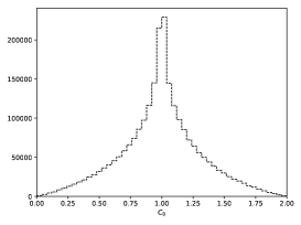
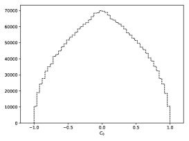
The amplitude of the $wt$ as function of $\alpha^{CP}$ depends on the multiplication of the length of the transverse components of the polarimetric vectors. The longitudinal component $h_{+}^{z}h_{-}^{z}$ is defining shift with respect to zero of the $wt$ mean value over a full (0, 2$\pi$) range. The maximum of the $wt$ distribution is reached for $\alpha^{CP}$ = $\measuredangle(h_{+}^{T},h_{-}^{T})$, the opening angle of transverse components of the polarimetric vectors.

The spin weight of formula (5) can be used to introduce transverse spin effects into the event sample when for the generation transverse spin effects were not taken into account at all. The above statement is true, independently if longitudinal spin effects were included and which $\tau$ decay channels complete cascade of $H\to\tau\tau$ decay. The shape of weight dependence on the Higgs coupling to $\tau$ parity mixing angle is preserved.

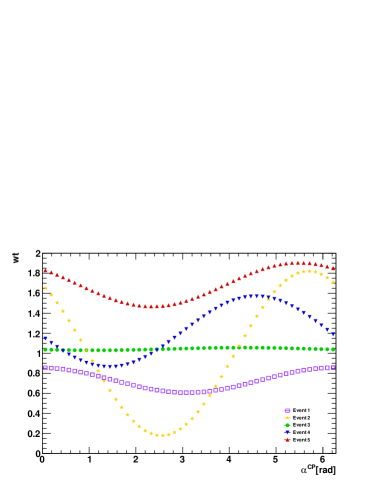
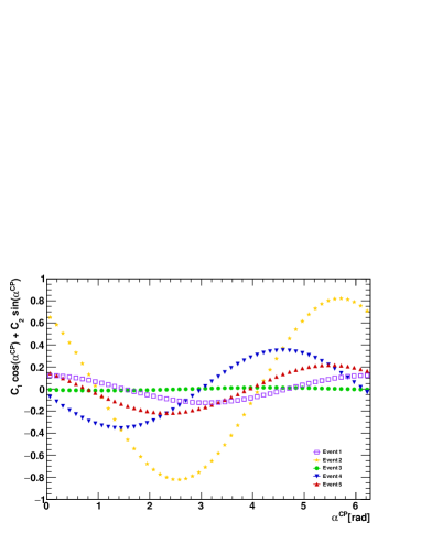
In Fig. 2 we show distribution of spin weight $wt$ for five example $H\to\tau\tau$ events collected in Table 1. For each event, depending on the polarimetric vectors, single value of $\alpha^{CP}$ is preferred (by the largest weight). For a physics model with $\alpha^{CP}$ the sample will be more abundantly populated with events for which the angle between polarimetric vectors, $\measuredangle(h_{+}^{T},h_{-}^{T})$, is close to $\alpha^{CP}$. We show distributions when complete polarimetric vectors are used for spin weight $wt$ and when only hadronic parts of polarimetric vectors are used. The second case is indicating easier to attain sensitivity part of observables. The $\alpha^{CP}$ at which spin weight has its maximum is then a bit shifted. Table 1 specifies values of the polarimetric vectors and the resulting coefficients $C_{i}$ calculated from formulas (2) and for events of Fig. 2. It also explicitly gives $\measuredangle(h_{+}^{T},h_{-}^{T})$ calculated from complete polarimetric vectors and (in brackets) from their hadronic parts only.

Table 1: Polarimetric vectors, resulting $C_{i}$ coefficients of formulas (2) and angle $\measuredangle(h_{+}^{T},h_{-}^{T})$ between transverse components of polarimetic vectors for five example events of $H\to\tau^{+}\tau^{-},\tau^{\pm}\to\rho^{\pm}\nu_{\tau}$. In brackets, angle of only hadronic part of polarimetric vector is given.

Events	Polarimetric vectors	$|h_{+}^{T}||h_{-}^{T}|$	$C_{0}$	$C_{1}$	$C_{2}$	$\measuredangle(h_{+}^{T},h_{-}^{T})$ [rad]
						(hadronic part only)
Event 1	$h_{+}^{x,y,z}$ = (0.7547 -0.2232 -0.6167)	0.7519	0.8179	0.7517	0.0183	6.2586
	$h_{-}^{x,y,z}$ = (-0.9093 -0.2931 -0.2953)					(6.1738)
Event 2	$h_{+}^{x,y,z}$ = (0.8617 0.0485 0.5050)	0.8535	1.0751	0.5518	-0.6511	5.4134
	$h_{-}^{x,y,z}$ = (-0.5959 0.7892 -0.1487)					(5.6307)
Event 3	$h_{+}^{x,y,z}$ = (0.3402 0.9377 -0.0682)	0.8339	0.9626	-0.1619	-0.8180	5.2130
	$h_{-}^{x,y,z}$ = (0.8262 0.1272 -0.5487)					(4.1923)
Event 4	$h_{+}^{x,y,z}$ = (-0.6964 0.6204 -0.3605)	0.4138	0.6769	-0.0919	-0.4035	4.4883
	$h_{-}^{x,y,z}$ = (0.2142 -0.3885 -0.8962)					(4.5127)
Event 5	$h_{+}^{x,y,z}$ = (0.1115 -0.4989 -0.8595)	0.1201	1.8354	0.0317	-0.1158	4.9793
	$h_{-}^{x,y,z}$ = (-0.2347 -0.01108 0.9720)					(5.4300)

Figure 2: The spin weight $wt$ (left plot) and only its $\alpha^{CP}$ dependent component (right plot) for five $H\to\tau\tau$ events of Table 1. Note the vertical scale change between left and right plots.

3 Monte Carlo samples and feature lists

For compatibility with our previous publications [16, 17], we use the same generated event samples, namely Monte Carlo events of the Standard Model, 125 GeV Higgs boson, produced in pp collision at 13 TeV centre-of-mass energy, generated with Pythia 8.2 [21] and with spin correlations introduced with TauSpinner [15] package. For $\tau$ lepton decays we use Tauolapp library [22]. All spin and parity effects are implemented with the help of weight $wt$ [23, 24]. The sample is generated without spin effects, and the spin weights $wt_{i}$ for few different values of CP mixing angle $\alpha^{CP}_{i}$ are stored. Spin weight, formula (3), is calculated using $R_{i,j}$ density matrix and polarimetric vectors $h_{\pm}$.

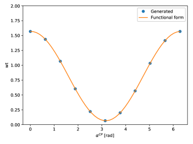
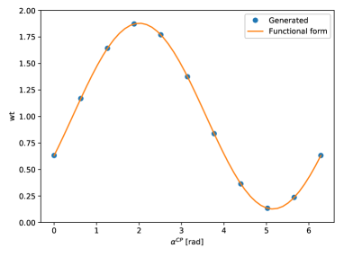
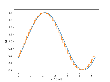
Later, for a given event it is possible to calculate coefficients $C_{0},C_{1},C_{2}$, using three $\alpha^{CP}$ and linear equation (5). Fig. 3 shows the cross-check how well this procedure works. The functional form (orange line) and evaluated spin weights (blue dots) for two example events are shown. The $C_{0},C_{1},C_{2}$ coefficients for the functional form are calculated solving Eq. (5) for $wt$ stored in the generated event samples at three values of $\alpha^{CP}$.

Figure 3: Cross-check distributions of the spin weight $wt$ calculated at generation (blue points) and from functional form of Eq. (5) (orange line), as a function of CP mixing parameter $\alpha^{CP}$. For left and right plots two different example events were used. Coefficients $C_{i}$ are reconstructed from eq. (5) and $wt$ is taken at three different $\alpha^{CP}$.

In this paper we present results for the case when both $\tau$’s decay $\tau^{\pm}\to\rho^{\pm}\nu_{\tau}$ and about $5\cdot 10^{6}$ simulated Higgs events are used. To partly emulate detector conditions, a minimal set of cuts is used. We require that the transverse momenta of the visible decay products combined, for each $\tau$, are larger than 20 GeV. It is also required that the transverse momentum of each $\pi^{\pm}$ is larger than 1 GeV.

The emphasis of the paper is to explore different ML approaches to the problem, and we discuss only the case of the Variant-All feature list from paper [17]. It contains the four-momenta of all decay products of $\tau$ leptons defined in the rest frame of intermediate resonance pairs, and with sum of hadronic decay products aligned with $z$-axis are. This represents an ideal benchmark case scenario, for performance monitoring.

4 Binary classification

The use of the DNN for binary classification have been discussed in our previous papers [16, 17]. The focus was on discriminating between CP-scalar ($\mathscr{H}_{0}$ hypothesis) and CP-pseudoscalar ($\mathscr{H}_{1}$ hypothesis).

Now we apply the same procedure but with alternative hypothesis ($\mathscr{H}_{\alpha^{CP}}$) representing the scalar-pseudoscalar mixed state of mixing parameter $\alpha^{CP}$. To quantify performance for Higgs CP state classification the weighted Area Under Curve (AUC) [25, 26] is used again. For each simulated event we know also Bayes optimal probability that it is sampled from $\mathscr{H}_{0}$ or $\mathscr{H}_{\alpha^{CP}}$ hypothesis, see more detailed description in Appendix A. This forms the so called oracle predictions, i.e. ultimate discrimination for this problem. We calculate oracle predictions and evaluate the results of DNN. This is a straightforward extension of the method used in [16, 17]. That is why, simple attempt on future discussion of systematic error may follow that suggested in [17]: variations within expected range of detector response can be easily introduced and biases studied.

The oracle predictions for discriminating between $\mathscr{H}_{0}$ and $\mathscr{H}_{\alpha^{CP}}$ hypotheses is increasing with $\alpha^{CP}$ and reach AUC=0.78 for $\alpha^{CP}=\pi$. The performance of DNN is following similar pattern, reaching maximum at $\alpha^{CP}=\pi$ (pure pseudo-scalar case). It decreases for smaller or larger $\alpha^{CP}$, where admixture of the scalar component appear. In case of complete feature list, it is almost achieving the performance of oracle predictions. In Fig. 4, the AUC values are plotted for full $\alpha^{CP}$ range. The distributions are (almost) symmetric around $\alpha^{CP}=\pi$. Note that the functional form of spin weight $wt$, Eq. (5), encapsulating sensitivity to $\alpha^{CP}$ is not symmetric, see Fig. 3. In Table 2 we show numerical results for few $\alpha^{CP}$.

Figure 4: The AUC score for binary classification between $\mathscr{H}_{0}$ and $\mathscr{H}_{\alpha^{CP}}$ hypotheses and corresponding oracle predictions.

Table 2: The AUC scores for discriminating between Higgs CP states. Results from oracle predictions and binary classification for discriminating between $\mathscr{H}_{0}$ hypothesis that Higgs CP is a scalar ( CP-mixing angle $\alpha^{CP}$ = 0.0 or 2$\pi$) and $\mathscr{H}_{\alpha^{CP}}$ hypothesis, when Higgs CP is of a parity mixed state, are shown. CP-mixing angle $\alpha^{CP}=\pi$ corresponds to pseudo-scalar case.

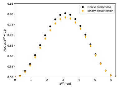
CP-mixing angle $\alpha^{CP}$	Oracle predictions	Binary
(units of $\pi$)		classification
0.2	0.528	0.525
0.4	0.605	0.595
0.6	0.699	0.684
0.8	0.775	0.756
1.0	0.804	0.784

5 Multiclass classification

The binary classification discussed in previous Section is easy to generalize to the multiclass case. The DNN is learning to provide per-event probabilities to associate with each class. Single class represents either discrete point or a specific range in 1-dimensional parameter space. We explore three approaches, each providing complementary physics information, but all allowing to quantify, on the per-event basis, which is the preferred mixing angle of the studied Higgs sample:

• The DNN classifier is learning per-event spin weight as a function of mixing angle $\alpha^{CP}$. The range of mixing angle $(0,2\pi)$ is discretised into equally spaced points called classes. This approach is described in Section 5.1, and used for the figures labeled with: Classification:wt.

• The DNN classifier is learning per-event coefficients $C_{0},C_{1},C_{2}$. The allowed range of coefficients is split into several equal size ranges (classes), single class represents a range for a coefficient value. The DNN is trained for each coefficient separately. This approach is described in Section 5.2 and used for the figures labeled with: Classification:$C_{0},C_{1},C_{2}$.

• The DNN classifier is learning per-event most probable mixing angle $\alpha^{CP}_{max}$, i.e. value of $\alpha^{CP}$ at which spin weight is maximal. The range of mixing angle $(0,2\pi)$ is split into several equally spaced points (classes). This approach is described in Section 5.3 and used for the figures labeled with: Classification:$\alpha^{CP}_{max}$.

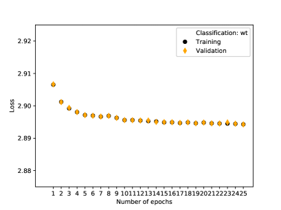
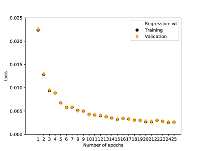
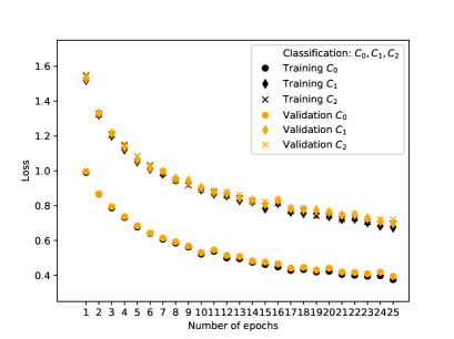
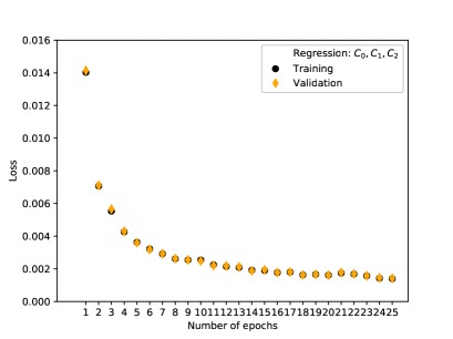
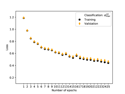
We monitor performance of the learning process in a standard manner, with the loss function on the training and validation sets. Respective distributions are shown in Fig. 20 of Appendix A. Note that the loss function, the tf.nn.softmax_cross_entropy_with_logits of the Tensorflow, allows to predict probabilities of the class labels, and not the actual value of the observable at a given class. In case of predicting spin weight distribution, only the normalized to unity shape is predicted. In case of predicting values of $C_{i}$ coefficients or $\alpha^{CP}_{max}$, vector of probabilities is returned, and the one-hot encoding transformation selecting most probable class is then applied to retrieve actual predicted value of the parameter.

5.1 Learning spin weight $wt$

The DNN classifier is trained with per-event feature list and as a label normalized to unity $N_{class}$-dimensional vector of spin weights $wt_{i}^{norm}=wt_{i}/\sum_{i=1}^{i=N_{class}}wt_{i}$ is given, each component of $wt^{norm}(\alpha^{CP})$ vector corresponds to the i-th discrete value of mixing angle $\alpha^{CP}_{i}$. $N_{class}$ denotes number of points to which range $(0,2\pi)$ was discretised. The number of classes is kept odd, to assure that $\alpha^{CP}=0,\pi,2\pi$, corresponding respectively to scalar/pseudoscalar/scalar cases, are always represented as a separate class. Training of DNN is performed with $N_{class}$ varying from 3 to 51. This is to understand the tradeoff between the better approximation given by high number of classes and smaller complexity of the low-class system.

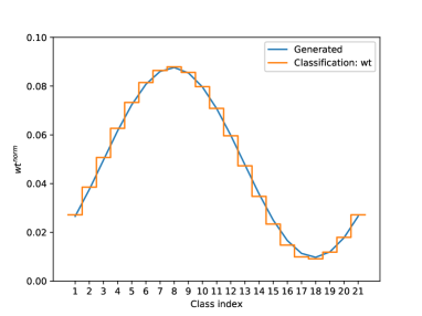
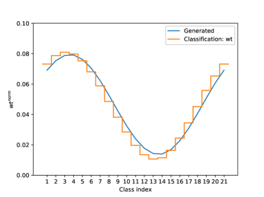
We quantify the DNN performance for classification problem in the context of physics relevant criteria. The first question is how well DNN is able to reproduce per-event shape of the spin weight $wt^{norm}$. For two example events, true and predicted spin weight $wt^{norm}$ distribution with $N_{class}=21$ is shown in Fig. 5 as a function of either continuous mixing parameter $\alpha^{CP}_{i}$ or class index i (representing discretised mixing parameter $\alpha^{CP}_{i}$). Blue line denote true weights while orange steps denote weights predicted by DNN classifier. In overall, predicted weights follow smoothly true shape of linear $\cos(\alpha^{CP})$ and $\sin(\alpha^{CP})$ combination. This is encouraging, because the loss function is not correlating explicitly nearby classes. The DNN is discovering this pattern in the process of learning.

Figure 5: Normalized to probability spin weight $wt^{norm}$, predicted (orange steps) and true (blue line), as a function of $\alpha^{CP}_{i}$ for two example events (left and right plots). DNN was trained with $N_{class}=21$ spanning range $(0,2\pi)$.

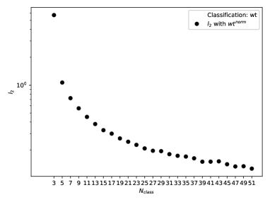
To quantify those observations, performance of DNN is monitored on the statistical basis with $l_{2}$ norm. The $l_{2}$ norm is defined as a square root of the integral of squared difference between predicted $p_{k}$ and true $wt^{norm}_{k}$ over the whole interval $(0,2\pi)$. It then averaged over the number of events $N_{evt}$. Although $p_{k}$ and $wt^{norm}_{k}$ are functions of $\alpha^{CP}$, we shall usually skip the argument for the notation brevity.

$$l_{2}=\sum_{k=1}^{N_{evt}}\frac{\sqrt{\int_{0}^{2\pi}\left(wt^{norm}_{k}(\alpha^{CP})-p_{k}(\alpha^{CP})\right)^{2}d\alpha^{CP}}}{N_{evt}}.$$ (7)

The $p_{k}$ corresponds to the k-th event and is represented as a step function, with step levels given by a $N_{class}$-dimensional output of DNN. For true weights, represented as continuous function (5), we scale them in such a way that $\int_{0}^{2\pi}wt^{norm}d\alpha^{CP}=1$, to enable the comparison. Distribution of $l_{2}$ norm is shown in Figure 6, as a function of class multiplicity $N_{class}$. With increasing number of classes, $l_{2}$ decreases. The slope remains very steep up to $N_{class}=21$, and seems to flatten around $N_{class}=51$. These two values of $N_{class}$ we’ve chosen as representative for the rest of the paper.

From physics perspectives, learning the shape of $wt$ distribution as function of $\alpha^{CP}$, is equivalent to learning components of the polarimetric vectors. But, because only the shape, not the normalization, is available the $C_{i}$ coefficients cannot be fully retrieved from formula (5). It is not necessary the aim anyway. The physics interest is more to learn $\alpha^{CP}$ which is preferred by events of the analyzed sample, i.e. value at which $wt$ distribution has its maximum. This corresponds to determining CP mixing angle of the analyzed sample.

Figure 6: The $l_{2}$ norm, quantifying difference between true and predicted spin weight $wt^{norm}$, as a function of class multiplicity $N_{class}$.

The second criterium is the difference between most probable predicted class and most probable true class, denoted as $\Delta_{class}$. When calculating difference between class indices, periodicity of the functional form (5) is taken into account. Class indices represent discrete values of $\alpha^{CP}$, in range $(0,2\pi)$. The distance between the first and the last class is zero. We take the distance which corresponds to the smaller angle difference and we take the sign according to clock-wise orientation vs class index at which true $wt$ has its maximum.

Let’s $idp_{max}$ denote the index of most probable predicted class, $idc_{max}$ be index of true most probable class. The distance $|\Delta_{class}|$ is defined as:

$$|\Delta_{class}|=min((|idp_{max}-idc_{max}|),((N_{class}-1)-|(idp_{max}-idc_{max})|)),$$ (8)

and the sign is attributed

$$\Delta_{class}=sign(idp_{max}-idc_{max})\ |\Delta_{class}|,$$ (9)

if $(|idp_{max}-idc_{max}|)<((N_{class}-1)-|(idp_{max}-idc_{max})|)$, or

$$\Delta_{class}=sign(idc_{max}-idp_{max})\ |\Delta_{class}|,$$ (10)

otherwise.

In Fig. 7 distributions of $\Delta_{class}$ for $N_{class}$ = 21 and 51 respectively are shown. The shapes are Gaussian-like and centered around zero. The mean <$\Delta_{class}$> = -0.006 [rad] in both cases and this we can interpret as the bias of the method. The standard deviation of per-event distribution is $\sigma_{\Delta_{class}}$ = 0.165 [rad] for $N_{class}$ = 21 and $\sigma_{\Delta_{class}}$ = 0.126 [rad] for $N_{class}$ = 51. As we can see, the performance has not improved significantly with $N_{class}$ exceeding 21.

Figure 7: Distribution of $\Delta^{max}_{class}$ between predicted most probable class and true most probable class for $N_{class}$ = 21 and 51 respectively. The mean and std are calculated in units of class index [idx] or units of radians [rad].

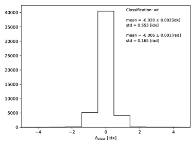
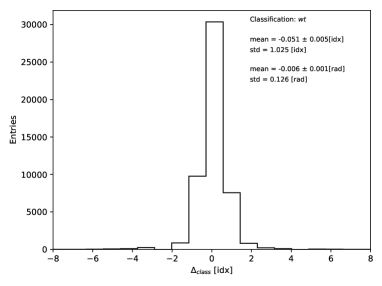
The DNN classifier which is predicting normalized spin weight $wt^{norm}$, provides enough information to identify the most probable mixing angle $\alpha^{CP}_{max}$ with high precision. The information is not sufficient though to reconstruct complete set of $C_{i}$ coefficients and the polarimetric vectors.

5.2 Learning $C_{0},C_{1},C_{2}$ coefficients

The second approach is to learn formula (5) coefficients $C_{0},C_{1},C_{2}$ for the spin weight $wt$. They can be then used to predict not only normalized $wt^{norm}$, but also original $wt$. Coefficients $C_{0},C_{1},C_{2}$ represent physical observables, products of longitudinal and transverse components of polarimetric vectors, as shown in formulas (2).

The classification technique using DNN is configured to learn each of the $C_{i}$ with separate training. The allowed range is well known, the $C_{0}$ spans the range (0.0, 2.0) and $C_{1},C_{2}$ the range (-1.0, 1.0), see Fig. 1. The allowed range is binned into $N_{class}$ and as a label, the $N_{class}$-dimensional vector with one-hot encoded value of the $C_{i}$ parameter is associated with each event. Therefore in this case, a single class represents range of the $C_{i}$ coefficient. During training, the DNN is learning per-event association between feature list and the class labels. The output is a probability $N_{class}$-dimensional vector, which is then converted to one-hot encoded representation, i.e. the most probable class is chosen as a predicted value of the $C_{i}$ coefficient.

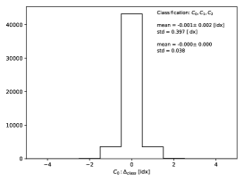
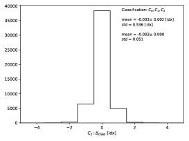
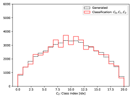
Distributions of the difference between true and predicted $C_{i}$ coefficients are shown in Figs. 8. In that case, as there is no periodicity involved, $\Delta_{class}=idp-idc$ where $idp$, $idc$ denote respectively true and predicted class index. Mean of $\Delta C_{i}$ is close to zero and standard deviation is of 0.038-0.051, which is less than 5% of the range. Precision with which $C_{i}$ coefficients are predicted is clearly limited by the $N_{class}$.

We use the true and predicted $C_{0},C_{1},C_{2}$ coefficients to calculate $wt$ distribution of (5). It is then discretised with $N_{class}$ points (the $N_{class}$ could be different than the one used for learning coefficients), and the $\alpha^{CP}_{max}$ is determined from the class of maximal weight. The difference between true and predicted $\alpha^{CP}_{max}$ is shown in Fig. 9 for $N_{class}$ = 21 and 51. The Gaussian-like shape of those distributions, centered around zero, clearly demonstrated that method works as expected. The mean and standard deviation of the distributions are close to those obtained with Classification:wt approach, of Fig. 7.

Figure 8: Difference between true and predicted coefficients $C_{0},C_{1},C_{2}$ of formula (5). For DNN training the granularity of $N_{class}$= 21 was used.

Figure 9: The difference between true and predicted most probable mixing angle $\alpha^{CP}_{max}$, calculated using formula (5) and coefficients $C_{0},C_{1},C_{2}$ learned with classification method. The granularity of $\alpha^{CP}_{max}$, $N_{class}$= 21 and 51 was used respectively for left and right-hand plot.

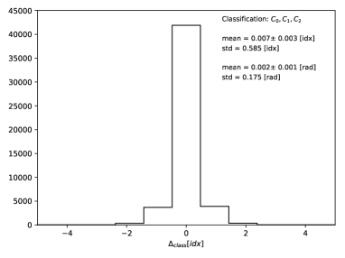
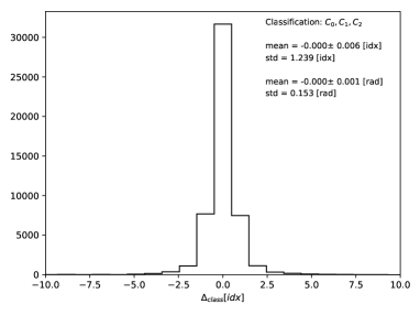
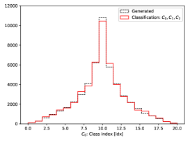
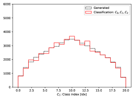
Finally, as sanity check we have compared the true distributions of $C_{0},C_{1},C_{2}$ with the predicted ones. As we can see in Fig. 10, both distributions match very well for all $C_{i}$.

Figure 10: Distributions of true and predicted coefficients $C_{0},C_{1},C_{2}$ of formula (5). For DNN training the granularity of $N_{class}$= 21 was used.

5.3 Learning the $\alpha^{CP}_{max}$

The third approach is to directly learn per-event most preferred mixing angle, $\alpha^{CP}_{max}$. The allowed range (0, 2$\pi$) is again binned into $N_{class}$ classes, where single bin represents discrete $\alpha^{CP}$. For training, for every event we take the one-hot encoded vector of $N_{class}$-dimension as a label. The DNN is returning $N_{class}$-dimensional vector of probabilities, which is then transformed into a single number, that is the class of the highest probability $\alpha^{CP}_{max}$. With this approach, neither spin weight nor $C_{i}$ coefficients are predicted.

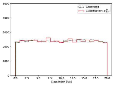
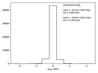
As the event sample is generated without any CP mixture favoured, the distribution of the $\alpha^{CP}_{max}$ is expected to be uniform, and such sanity check is demonstrated in the left plot of Fig. 11. The DNN is well reproducing this behaviour. The $\Delta\alpha^{CP}_{max}$, the difference between true and predicted value of the $\alpha^{CP}_{max}$ is shown in the right plot of Fig. 11. In the case of $N_{class}$ = 21, it has a Gaussian-like shape with the mean $<\Delta\alpha^{CP}_{max}>$ = 0.003 $\pm$ 0.001 [rad] and standard deviation 0.139 [rad]. Results are again comparable with the ones obtained with the previously discussed approaches.

Figure 11: Distributions (left-hand plot) of true and predicted most preferred mixing angle $\alpha^{CP}$. The distribution of per-event difference of the two is shown on the right-hand plot. The granularity of $N_{class}$= 21 was used for training DNN.

6 Regression

The ML regression is not so commonly used in the high energy physics analyses. The main feature is, that contrary to the classification case, we get a continuous parameter (or set of parameters) as a DNN output. We explore three approaches, defined similarly as in Section 5

• The DNN is learning to predict per-event spin weight as a function of mixing angle $\alpha^{CP}$. The range of mixing angle $(0,2\pi)$ is split into discrete points of $\alpha^{CP}$ at which value of spin weight is learned. This approach is described in Section 6.1 and used for the figures labeled with: Regression:wt.

• The DNN is learning to predict per-event value of the coefficients $C_{0},C_{1},C_{2}$ of the functional form (5). The DNN is trained for all coefficients simultaneously. This approach is described in Section 6.2 and used for the figures labeled with: Regression:$C_{0},C_{1},C_{2}$.

• The DNN is learning to predict per-event most probable mixing angle $\alpha^{CP}_{max}$, i.e. where $\alpha^{CP}$ spin weight has maximum. This approach is described in Section 6.3 and used for the figures labeled with: Regression:$\alpha^{CP}_{max}$.

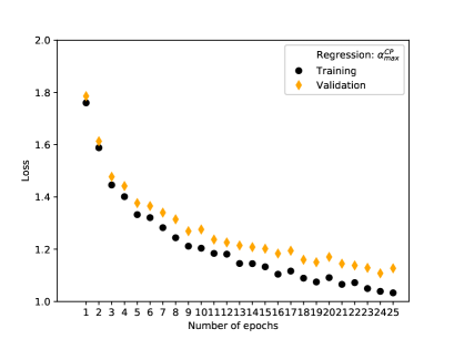
We continue with Tensorflow package, but now with tf.losses.mean_squared_error function as a loss in the training procedure of Section 6.1, 6.2 and self-defined function in the training procedure of Section 6.3. Mentioned self-defined function is discussed in the appendix.

6.1 Learning spin weight $wt$

Similarly as in the classification case, the DNN regression is trained on an input information consisting of per-event feature list. As a training output we provide a vector of the spin weight $wt_{i}$ for the discrete values of $\alpha^{CP}$. Training is performed for different granularities of $\alpha^{CP}$ discretisation, to monitor performance sensitivity. Again in this case we use odd number of equally spaced points $\alpha_{i}^{CP}$, so the $\alpha^{CP}=0,\pi,2\pi$ coincide with a single point. It is worth noting, that in case of regression, both shape and normalization of the $wt$ are learned by the DNN.

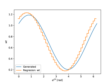
For two example events in Fig. 12, true continuous spin weight $wt$ distribution as well as step-function prediction is shown as a function of mixing parameter $\alpha^{CP}$. In overall, predicted weights follow smoothly expected shape of linear $\cos(\alpha^{CP})$ and $\sin(\alpha^{CP})$ combination, even if no attempt to regularize for such smooth behaviour was made.

Figure 12: Example plots with DNN regression results: the spin weight $wt$, predicted (orange steps) and true (blue line), as a function of $\alpha^{CP}_{i}$ for two example events (left and right plots). DNN was trained with $N_{class}=51$ spanning range $(0,2\pi)$.

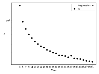
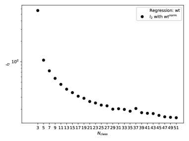
Distributions of $l_{2}$ norm, defined in the same way as in the classification case, as a function of $N_{class}$ (granularity for discretising $\alpha^{CP}$) is shown in Figure 13. For more compatibility with the classification case of Section 5.1 we present results for original $wt$, as well as normalized to unity $wt^{norm}$. The results are comparable, with a visible flattening of $l_{2}$ for higher values of $N_{class}$.

Figure 13: The $l_{2}$ norm for predicted spin weight $wt$ (left) and $wt^{norm}$ (right) as a function of $N_{class}$.

Figure 14: Distribution of $\Delta_{class}$ between most probable predicted class and true most probable class. The $N_{class}$ = 21 and 51 are used for respectively left and right plot. The mean and std standard deviation are calculated in units of class index [idx] and units of radians [rad].

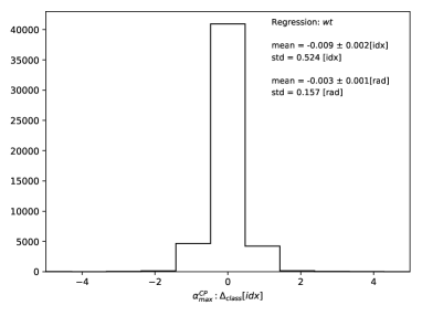
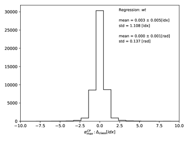
In Fig. 14 distributions of $\Delta_{class}$ for $N_{class}$ = 21 and 51 used to train DNN regression are respectively shown. The shape is Gaussian-like and as expected centered around $\Delta_{class}$=0.

6.2 Learning $C_{0},C_{1},C_{2}$ coefficients

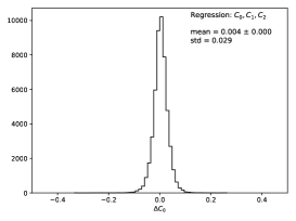
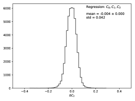
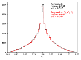
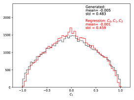
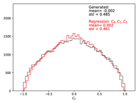
Regression approach allows us to predict $C_{0},C_{1},C_{2}$ coefficients directly, without any need of discretization. The differences between true and predicted ones are shown in Figs. 15. On average, all three coefficients are predicted reasonably well. Consistent are the statistical summaries of $\Delta C_{i}$: means remain in the range $\pm 0.004$ and standard deviations in range (0.029-0.042). Coefficients $C_{i}$ are then used to calculate predicted spin weight $wt$ of formula (5).

We have investigated also, how well predicted $C_{0},C_{1},C_{2}$ can be used to estimate the most preferred mixing angle, $\alpha^{CP}_{max}$. For consistency, we evaluate it using the same criteria as for classification approaches. This is achieved by using coefficients $C_{0},C_{1},C_{2}$ to calculate spin weight $wt$, and then turning it into discrete predictions for $wt$ and $wt^{norm}$ in the $N_{class}$ points. As in Section 5 for classification approach, we use $\Delta_{class}$, defined by formulas (8) -(10).

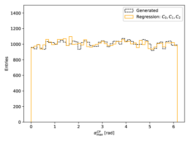
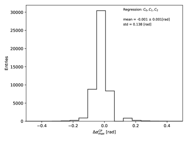
The distributions of the true and predicted most probable class, $\alpha^{CP}_{max}$ and their difference are shown in Figs. 16 for the $N_{class}$ = 51. We expect the distributions to be flat as sample was generated without any polarization correlation (carrier of CP effects) included, and this sanity check seems to be positive. The difference between true and predicted $\alpha^{CP}_{max}$ forms a narrow peak with the mean value $<\Delta\alpha^{CP}_{max}>~{}=~{}-0.001\pm 0.001$ [rad] and standard deviation 0.138 [rad].

Finally, as a sanity check, we have compared the true overall distribution of $C_{0},C_{1},C_{2}$ with the predicted one. As we can see in Fig. 10, both distributions match very well.

Figure 15: Difference between true and predicted coefficients $C_{0},C_{1},C_{2}$ of formula (5).

Figure 16: Distributions (left plot) of true (black dashed line) and predicted (orange line) most preferred mixing angle $\alpha^{CP}$. The prediction was based on coefficients $C_{0},C_{1},C_{2}$. The distribution of per-event difference of the two is shown on the right plot.

Figure 17: Distributions of true and predicted coefficients $C_{0},C_{1},C_{2}$ of formula (5).

6.3 Learning the $\alpha^{CP}_{max}$

As was in the previous subsection, the implementation of the regression method allows a direct, non-discrete estimation of continuous parameters. This is also desired with the most preferred mixing angle $\alpha^{CP}_{max}$.

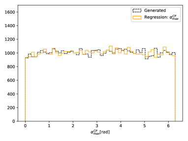
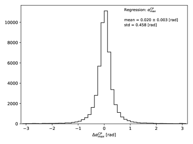
The distributions of the true and predicted most probable class, $\alpha^{CP}_{max}$ and their difference are shown in Figs. 18 for the $N_{class}$ = 51. We expect the distributions to be flat as sample was generated without any polarization correlation (carrier of CP effects) included, and this sanity check seems to be positive. As the used event sample is generated without any polarization, the distribution of the $\alpha^{CP}_{max}$ is expected to be uniform, see the left plot of Fig. 18. The DNN is reproducing this feature well. The difference between true and predicted $\alpha^{CP}_{max}$ forms a narrow peak with the mean $<\Delta\alpha^{CP}_{max}>=0.020\pm 0.003$ [rad] and standard deviation 0.458 [rad].

Figure 18: Distributions (left plot) of true (black dashed line) and predicted (orange line) most preferred mixing angle $\alpha^{CP}$. The distribution of per-event difference of the two is shown on the right plot.

7 Classification or regression: comparison and complementarity

In this Section we shortly compare classification and regression approaches. In Table 4 we collect the mean and standard deviation for difference between true and predicted with classification and regression methods $C_{i}$. There is no clear winner, both methods give predictions of similar precision, with only $C_{0}$ being better predicted with regression.

In Table 4 we compare the difference between true and predicted $\alpha^{CP}_{max}$ obtained with different methods. With the classification method comparable performance is achieved when learning spin weight $wt$, coefficients $C_{0},C_{1},C_{2}$ or directly $\alpha^{CP}_{max}$. For the regression method learning directly $\alpha^{CP}_{max}$ is significantly less performant. Otherwise, is no clear winner between different methods.

Table 3: The mean and standard deviations of $\Delta C_{i}$, the difference between generated and predicted $C_{i}$, obtained from DNN with classification and regression methods for $N_{class}=51$.

Coefficients	Classification	Regression
$\Delta C_{0}$	mean = 0.000	mean = 0.004
	std = 0.038	std = 0.029
$\Delta C_{1}$	mean = 0.001	mean = -0.004
	std = 0.051	std = 0.042
$\Delta C_{2}$	mean = -0.003	mean = -0.04
	std = 0.051	std = 0.042

Table 4: The mean and standard deviation of $\Delta\alpha^{CP}_{max}$, the difference between true and predicted $\alpha^{CP}_{max}$, obtained from DNN with classification and regression methods.

Method	Classification	Regression
Using $wt$	mean = -0.006 $\pm$ 0.001 [rad]	mean = 0.000 $\pm$ 0.001 [rad]
	std = 0.126 [rad]	std = 0.137 [rad]
Using $C_{0},C_{1},C_{2}$	mean = 0.000 $\pm$ 0.001 [rad]	mean = -0.001 $\pm$ 0.001 [rad]
	std = 0.153 [rad]	std = 0.138 [rad]
Direct	mean =- 0.003 [rad]	mean = 0.020 [rad]
	std = 0.139 [rad]	std = 0.458 [rad]

8 Summary

We have performed a proof-of-concept for the DNN methods in the measurement of Higgs boson $H\to\tau\tau$ CP mixing angle dependent coupling. That extends work of refs. [16, 17] of classification between scalar and pseudoscalar Higgs CP state. Several solutions of classification and of regression types were prepared and numerical results were collected. For the measurement we have studied approaches where; (i) spin weights, (ii) coefficients for the functional form of the spin weight (iii) directly the mixing angle at which the weight has its maximum, were targeted. In cases (i) and (ii) the classification approach seemed comparable to the regression, but the comparisons relied on the discretised and normalized quantities due to classification limitations. The regression approach seems more natural for continuous observables and does not have such limitations. On the other hand, regression approach has performed much worse in the case of direct $\alpha^{CP}_{max}$ prediction.

For the feature list we have chosen idealistic case, assuming that complete set of $\tau$ decay products 4-momenta is known, including challenging to reconstruct neutrinos. We have exploited then the $\tau\to\rho\nu$ decay mode. The results are encouraging, the understanding of environment for future discussion of measurement ambiguities was not compromised with respect to what was achieved in previous publications for scalar/pseudoscalar classifications.

The mean value of the preferred mixing angle $\alpha^{CP}_{max}$ can be constrained by the trained DNN with per-event resolution better than 0.15 [rad] using a classification approach. Both classification and regression approaches allow to learn spin weight with uncertainties (average $l_{2}$ norm) better than 15%. Both approaches allow also to learn coefficients $C_{0},C_{1},C_{2}$ of the functional spin weight form. The coefficients are directly related to the polarimetric vectors of decaying $\tau^{\pm}$ leptons. This provides interesting possibility for the future studies of experimental ambiguities with samples of the $Z\to\tau\tau$ decays, much more abundant and available for the LHC measurements. Departure from SM predictions on $Z\tau\tau$ coupling can reveal itself in the observables build from polarimetric vectors of decaying $\tau^{\pm}$ leptons too.

We plan, following [16, 17], to extend our studies to more realistic feature lists and other decay modes. Already now, the variety of ML methods for the determination of most preferred CP state mixing angle, demonstrated potential and robustness for future experimental analyses and measurements with the LHC data.

Acknowledgments

We would like to thank J. Kurek and P. Winkowska for help with technical implementation and testing of the analysis code used for this paper preparation.

Appendix A Deep Neural Network

The structure of the simulated data and the DNN architecture follows what was published in our previous papers [16, 17]. It is prepared for TensorFlow [27], an open-source machine learning library.

We consider $H\to\tau\tau$ channel of both $\tau^{\pm}\to\rho^{\pm}\nu$ decay. The data point is thus an event of the Higgs boson production and $\tau$ lepton pair decay products. The structure of the event is represented as follows:

$$x_{i}=(f_{i,1},...,f_{i,D}),w_{a_{i}},w_{b_{i}},...,w_{m_{i}}$$ (11)

The $f_{i,1},...,f_{i,D}$ represent numerical features and $w_{a_{i}},w_{b_{i}},w_{m_{i}}$ are weights proportional to the likelihoods that an event comes from a class $A,B,...,M$, each representing different $\alpha^{CP}$ mixing angle. The $\alpha^{CP}=0,2\pi$ corresponds to scalar CP state and $\alpha^{CP}=\pi$ to pseudoscalar CP state. The weights calculated from the quantum field theory matrix elements are available and stored in the simulated data files. This is a convenient situation, which does not happen in many other cases of ML classification. The $A,B,...M$ distributions highly overlap in the $(f_{i,1},...,f_{i,D})$ space, the more detailed discussion in case of two hypotheses only, scalar and pseudoscalar, can be found in [16].

Thanks to similar DNN architecture, we have prepared three implementations for measuring Higgs boson CP state: binary classification, multiclass classification and regression:

• For binary classification the aim is to discriminate between two hypothesis, $\mathscr{H}_{0}$ and $\mathscr{H}_{\alpha^{CP}}$.

• For multiclass classification, the aim is to simultaneously learn weights (probabilities) for several $\mathscr{H}_{\alpha^{CP}}$ hypotheses; learn coefficients of the weight functional form or directly learn the mixing angle at which spin weight has its maximum, $\alpha^{CP}_{max}$. A single class can be either single discretised $\alpha^{CP}$ or a range for the $C_{i}$ parameters. The system is learning probabilities for classes to associate with the event.

• For regression case, the aim is similar as for multiclass classification case, but now problem is defined as a continuous case. The system is learning value to associate with the event. The value can be a vector of spin weights for a set of $\mathscr{H}_{\alpha^{CP}}$ hypotheses, set of $C_{i}$ coefficients or $\alpha^{CP}_{max}$.

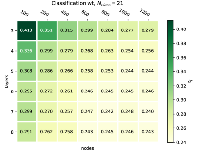
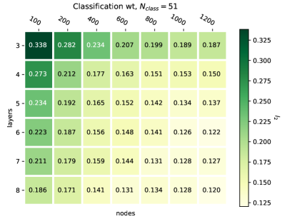
The network architecture consists of 6 hidden layers, 1000 nodes each with ReLU activation functions and is initialized with random weights. Such architecture has been found as a good tradeoff between the performance and computation time, what can be seen in Fig. 19. Learning procedure is optimized using a variant of stochastic gradient descent algorithm called Adam [28] and Batch Normalization [29].

Figure 19: Performance of $wt$ fitting ($l_{2}$) for different number of layers and nodes, assuming $N_{class}$= 21 (left-side) and $N_{class}$= 51 (right-side).

The last layer is specific to the implementation case, different is dimension of the output vector, activation function and a loss function. In the following, we will describe details.

Classification: The loss function used in stochastic gradient descent is a cross entropy of valid values and neural network predictions [4]. It is a common choice in case of binary or multiclass classification models. The loss function for sample of $N_{evt}$ events and classification for $N_{class}$ reads as follows:

$$Loss=\sum_{k=1}^{N_{evt}}\sum_{i=1}^{N_{class}}y_{i,k}log(p_{i,k}),$$ (12)

where $k$ stands for consecutive event and $i$ for class index. The $y_{i,k}$ represents neural-network predicted probability for event $k$ being of class $i$ while $p_{i,k}$ represents true probability used in supervised training.

Regression: In case of predicting $wt$ the last layer of DNN is $N$ dimensional output (granularity with which we want to discretise it). For predicting $C_{0},C_{1},C_{2}$ the last layer of DNN is N=3 dimensional output, i.e. values of $C_{0},C_{1},C_{2}$. Activation of this layer is a linear function. Loss functions is defined as Mean Squared Error (MSE) between true and predicted parameters

$$Loss=\sum_{k=1}^{N_{evt}}\sum_{i=1}^{i=N}(y_{i,k}-p_{i,k})^{2},$$ (13)

where $k$ stands for event index and $i$ for index of function form parameter. The $y_{i,k}$ represents predicted value of $C_{i}-th$ parameter for event $k$ while $p_{i,k}$ represents true value. For predicting the $\alpha^{CP}_{max}$ the last layer of DNN is N=1 dimensional output, i.e. values of $\alpha^{CP}_{max}$.

The tf.reduce_mean method of TensorFlow is used, with the loss function

$$Loss=\sum_{k=1}^{N_{evt}}(1-cos(y_{k}-p_{k})),$$ (14)

where $y_{k},p_{k}$ denotes respectively predicted and true value of $\alpha^{CP}_{max}$.

In Fig. 20, for all problems considered, distributions of the loss functions on the training and validation samples, as a function of number of epochs used for training are shown. Left plots are for the classification and right plots for the corresponding regression. The values of the loss are case specific and should not be directly compared, their shape is monitoring the training process. For all cases the loss is decreasing with number of epochs, both on training and validation samples. It is overlapping for all cases except [Regression:$\alpha^{CP}_{max}$] (bottom right plot), for that single case one small loss in performance is observed for validation sample compared to training sample. Training with 25 epochs seems sufficient for both classification and regression for all presented scenarios.

Figure 20: The DNN loss for classification (left-side) and regression (right-side), as function of number of epochs used for training. It is shown for learning spin weight (top plots), $C_{i}$ coefficients (middle plots) and most likely mixing angle $\alpha^{CP}_{max}$ (bottom plots). For the classification, $N_{class}$= 21 was used.

References

- [1] D. Guest, K. Cranmer, and D. Whiteson, 1806.11484.
- [2] G. Carleo, I. Cirac, K. Cranmer, L. Daudet, M. Schuld, N. Tishby, L. Vogt-Maranto, and L. Zdeborová, 1903.10563.
- [3] K. Albertsson et al., 1807.02876.
- [4] I. Goodfellow, Y. Bengio, and A. Courville, Deep learning. MIT Press, Cambridge, MA, 2017.
- [5] J. Lee, N. Chanon, A. Levin, J. Li, M. Lu, Q. Li, and Y. Mao, Phys. Rev. D99 (2019), no. 3 033004, 1812.07591.
- [6] J. Searcy, L. Huang, M.-A. Pleier, and J. Zhu, Phys. Rev. D93 (2016), no. 9 094033, 1510.01691.
- [7] S. Forte, L. Garrido, J. I. Latorre, and A. Piccione, JHEP 05 (2002) 062, hep-ph/0204232.
- [8] M. Kramer, J. H. Kuhn, M. L. Stong, and P. M. Zerwas, Z. Phys. C64 (1994) 21–30, hep-ph/9404280.
- [9] G. R. Bower, T. Pierzchala, Z. Was, and M. Worek, Phys. Lett. B543 (2002) 227–234, hep-ph/0204292.
- [10] A. Rouge, Phys. Lett. B619 (2005) 43–49, hep-ex/0505014.
- [11] K. Desch, Z. Was, and M. Worek, Eur. Phys. J. C29 (2003) 491–496, hep-ph/0302046.
- [12] S. Berge and W. Bernreuther, Phys. Lett. B671 (2009) 470–476, 0812.1910.
- [13] S. Berge, W. Bernreuther, and S. Kirchner, Phys. Rev. D92 (2015) 096012, 1510.03850.
- [14] ATLAS Collaboration, ATL-PHYS-PUB-2019-008 .
- [15] T. Przedzinski, E. Richter-Was, and Z. Was, Eur. Phys. J. C74 (2014), no. 11 3177, 1406.1647.
- [16] R. Jozefowicz, E. Richter-Was, and Z. Was, Phys. Rev. D94 (2016), no. 9 093001, 1608.02609.
- [17] K. Lasocha, E. Richter-Was, D. Tracz, Z. Was, and P. Winkowska, 1812.08140.
- [18] Abadi Martın, et.al. Software available from tensorflow.org (2015).
- [19] K. Desch, A. Imhof, Z. Was, and M. Worek, Phys. Lett. B579 (2004) 157–164, hep-ph/0307331.
- [20] E. Barberio, B. Le, E. Richter-Was, Z. Was, D. Zanzi, and J. Zaremba, Phys. Rev. D96 (2017), no. 7 073002, 1706.07983.
- [21] T. Sjöstrand et al., Comput. Phys. Commun. 191 (2015) 159 doi:10.1016/j.cpc.2015.01.024 [arXiv:1410.3012 [hep-ph]].
- [22] N. Davidson, G. Nanava, T. Przedzinski, E. Richter-Was, and Z. Was, Comput.Phys.Commun. 183 (2012) 821–843, 1002.0543.
- [23] Z. Czyczula, T. Przedzinski, and Z. Was, Eur.Phys.J. C72 (2012) 1988, 1201.0117.
- [24] T. Przedzinski, E. Richter-Was, and Z. Was, Eur. Phys. J. C79 (2019), no. 2 91, 1802.05459.
- [25] A. P. B. Bradley, Pattern recognition 30 (1997) 1145.
- [26] T. Fawcett, Pattern Recognition Letters 27 (2006), no. 7 861.
- [27] M. Abadi, A. Agarwal, P. Barham, E. Brevdo, Z. Chen, C. Citro, G. S. Corrado, A. Davis, J. Dean, M. Devin, et al., Software available from tensorflow. org 1 (2015).
- [28] D. Kingma and J. Ba, arXiv:1412.6980 (2014).
- [29] S. Ioffe and C. Szegedy, arXiv:1502.03167 (2015).