Estimation of roughness measurement bias originating from background subtraction
Abstract
When measuring the roughness of rough surfaces, the limited sizes of scanned areas lead to its systematic underestimation. Levelling by polynomials and other filtering used in real-world processing of atomic force microscopy data increases this bias considerably. Here a framework is developed providing explicit expressions for the bias of squared mean square roughness in the case of levelling by fitting a model background function using linear least squares. The framework is then applied to polynomial levelling, for both one-dimensional and two-dimensional data processing, and basic models of surface autocorrelation function, Gaussian and exponential. Several other common scenarios are covered as well, including median levelling, intermediate Gaussian–exponential autocorrelation model and frequency space filtering. Application of the results to other quantities, such as Rq, Sq, Ra and Sa is discussed. The results are summarized in overview plots covering a range of autocorrelation functions and polynomial degrees, which allow graphical estimation of the bias.
Keywords: Scanning probe microscopy; data processing; roughness; bias; levelling; autocorrelation
1 Introduction
Surface roughness is a ubiquitous phenomenon which influences many interactions of an object with outer world—mechanical [1, 2, 3], optical [4, 5, 6], chemical [7], biological [8], and others. Its influence is particularly large in the nanoscience and nanotechnology fields, where object sizes are comparable to characteristic dimensions of roughness (height and/or lateral) which arise naturally during deposition and processing of materials. Whether roughness is considered a defect to be minimized or potentially useful property to be optimized, it must be measured. Scanning Probe Microscopy (SPM) techniques, such as Atomic Force Microscopy (AFM), allow direct measurement of nanoscale roughness—while optical techniques allow its characterisation in the frequency domain [9]. Larger-scale roughness can be measured by profilometry techniques, of which mechanical profilometry in some sense analogous to SPM.
Two approaches to measurement should be distinguished. In an industrial context reproducibility is key and thus the focus is on procedures and parameters defined by standards [10, 11, 12, 13]. It may be of less concern if these parameters are those occurring in theoretical models or if they correspond to parameters of a hypothetical random process. On the other hand, in basic research the instruments, methods and samples are frequently all non-standard. Simultaneously, it is important to estimate parameters that correspond to theoretical descriptions. This can be either because they are themselves interesting, for instance in determining the universality class for a growth mechanism [14, 9]. Or they appear in physical theories describing interactions with rough surfaces. Probably the most interesting parameter is squared mean square roughness which directly appears in optics—together with similar quadratic quantities such as spectral densities of spatial frequencies and (cross)correlation functions [4, 15, 16]. Here we will approach roughness from this second standpoint.
Surface roughness is never measured using data from an infinitely large region with infinite resolution. The resolution is always finite—in contact scanning methods (AFM or profilometry) limited by finite probe size, in optical methods by finite wavelength. The measurement area is also always finite and seldom even encompasses the entire sample, in particular in direct measurements. In fact, in AFM we regularly measure tiny fractions of the surface—and instead of rigorous statistical justification for representativeness of the results we just have hope that no evil forces conspired to plant non-representative surface regions under the probe.
Still, conceptually, the statistical character of roughness parameters is acknowledged [9, 17]. We imagine an infinite ensemble of surfaces (possibly infinite themselves), usually corresponding formally to a random process, which may or may not be wide-sense stationary. Measurement of non-stationary fractal surfaces in an interval of scales in which they do exhibit self-affinity adds its own set of difficulties [9, 18]. Here we will focus on roughness generated by stationary processes—and estimation of their parameters using a finite measurement of one realization. In particular, we will study the consequences of finite measurement area and levelling/background subtraction.
One obvious consequence is that the estimated parameter, for example mean square roughness , estimated from a profile of length by
| (1) |
is itself a random variable, as we denote with a hat. It has a dispersion, which is possibly large [9]. Definition (1) corresponds to mean square roughness Rq for profiles [10, 11, 13] and Sq for images [19] defined by roughness measurement standards, with the subtle conceptual difference discussed above.
The estimate is also biased. Heights entering (1) are levelled to have zero mean value. This alone introduces bias, which is well known and discussed for correlated data in classical signal processing textbooks [20, 9, 21, 22]. However, subtraction of the mean value is rarely the only preprocessing applied to topographical data before roughness evaluation. Often local defects are removed first, although this may be unnecessary as evaluation algorithms for irregular regions allow excluding arbitrary image parts from processing [23]. Almost universally the mean plane is subtracted to correct tilt—and frequently not just a plane but a higher order polynomial to correct scanner bow (or sample warping) [17]. Misaligned scan lines need to be aligned for 2D processing, although not necessarily for line-by-line evaluation. Furthermore, any of specific form removal methods can be utilized, from frequency-space filtering to wavelet processing to subtraction of specific geometrical shapes such as sphere.
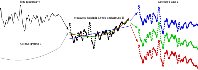
Some of these steps remove background arising from measurement imperfections (scanner bow), some remove real base shape of the measured object. Often they remove both to some degree—and by intentionally removing certain degrees of freedom they also always remove inadvertently a part of the roughness. For instance in the case of the mean value, we subtract it because the measured surface height is not the roughness signal . It is offset by some background, in this case a constant base height :
| (2) |
The background is non-random (at least from the roughness standpoint), but unknown. We estimate it as the mean value of the heights
| (3) |
because the expected value of is . However, the subtraction of instead of true removes not just but also a part of the roughness. Although the expected value of is zero, the mean value of over a finite interval is a random variable, not zero—yet we make it zero anyway.
This is illustrated in (1) for a second-order polynomial . A second-order polynomial background was added to an ‘ideal’ rough signal. Then a polynomial background was fitted and removed. We seldom know the exact background type and each choice levels the surface differently. Furthermore, even if the correct degree is chosen, the levelled surface differs from the original ideal one.
As already noted above, real AFM or profilometry data are sets of discrete values , not continuous functions . Integrals such as (1) or (3) are approximated by summations, for instance
| (4) |
There is a certain arbitrariness in the correspondence between the region and the set of points where heights were measured. If we state that were obtained in the centres of sampling steps (or pixel centres for images), the ‘measured region’ covers and extends a further half-step to each side. Formula (4) then becomes the midpoint quadrature rule [24] with only second-order error and approximates well the integral as long as the sampling step is small compared to the autocorrelation length . Since this work focuses on the effect of finite measurement area, i.e. loss of low-frequency information, we will not dwell on the loss of high-frequency information and will assume the sampling is sufficiently fine. Therefore, continuous functions will be used in the following analysis (instead of sets of discrete sampled values ).
2 Mean value subtraction
The root mean square roughness is estimated from heights in a finite-size region
| (5) |
For simplicity, we will consider one-dimensional (1D) data here.
The formula for is now always presented with explicit subtraction of of . Instead we simply say that ‘the mean value of heights is zero’. However, this confounds two distinct statements:
-
•
the expected value of roughness signal is zero , and
-
•
the mean value of measured data is made zero by preprocessing.
The second is the source of bias since is a random variable, not identically equal to zero even when its expected value is: .
We now briefly reproduce the classical result for the bias caused by mean value subtraction [20, 9, 21, 22]. The derivation provides an outline for how the more complex cases will be treated in section 3. Expanding the square in (5) gives
| (6) |
We would like to know the expected value of the estimate . The expected value of the first term on the right hand side of (6) is . Hence the second term gives the bias—which is always negative. Writing
| (7) |
and using coordinate transformation we obtain
| (8) |
Expected value calculation can be interchanged with integration. The expected value of either integrand is the autocorrelation function (ACF) of the signal
| (9) |
Note that . Substituting this result into (6) gives the classic final expression [20, 21]
| (10) |
Since the bias is always negative and proportional to , it is convenient to introduce the relative bias
| (11) |
to simplify notation. If we know , replacing with corrects the bias.
In order to see how the bias typically behaves, we evaluate it for a simple prabolic model of ACF for and zero otherwise. Then for
| (12) |
in one and two dimensions, respectively. The approximations hold for small. The numerical factors such as and change somewhat with the exact form of the ACF, but generally are of the same order of magnitude.
The important point is that the relative systematic error of due to finite-area bias behaves approximately as and for 1D and 2D data, respectively. More generally, it behaves like where denotes the dimension [9]. It does not depend on the number of measured values (provided it is sufficiently large). Increasing without making the measurement area larger is of no help and Bessel’s correction
| (13) |
which replaces with is ineffective. For correlated data the correction factor is not , but akin to or , where is some constant of order of unity.
Almost all roughness measurements involve correlated data. If we measure with such a large sampling step that the height values are uncorrelated we lose all spatial information about the roughness. This is rarely desirable—and also rarely possible, since in scanning methods the feedback loop then cannot keep up with the surface topography, whereas in optical methods this usually means averaging too large regions of the surface in one pixel.
3 Real-world background subtraction
Background subtraction methods used for SPM are much more complex than mere mean value subtraction [25, 26, 27, 17]. In order to evaluate roughness correctly, we must take into account which degrees of freedom or spatial frequencies would contribute to the desired result, but were removed by preprocessing. This is not trivial to start with and certainly not helped by AFM data processing software, which can apply plane levelling or row alignment automatically, possibly without the user even noticing (depending on the software and settings). And, of course, no AFM software currently attempts to estimate the resulting bias.
It is common to process AFM image data row by row because roughness properties can often be determined more reliably in the direction of the fast scanning axis [28, 9, 23, 17]. This means that levelling is applied to individual image rows instead of (or in addition to) the entire image. The operation of mutual alignment of scan lines is colloquially referred to as ‘flatten’ [25, 26, 27]. However, we explicitly call it scan line correction for clarity.
Results for individual rows then may be summed or averaged. The result for each row is biased as if we processed 1D data, not 2D. The same holds if any row-wise preprocessing is applied, such as removal of mean value from each individual row. It is, therefore, quite rare that the bias corresponds to the 2D case, even for image data.
3.1 Linear-fit background
Removal of tilt, bow or higher order polynomial backgrounds has two basic steps. Fitting a background function to the data using the linear least squares method, and subtraction of the fitted (estimated) background . This section presents a general framework for evaluating bias resulting from background subtraction by linear fitting. Not all background removal methods are linear—for instance the subtraction of median or a fitted spherical surface is non-linear, but most common ones are.
A linear fitting function satisfies
| (14) |
where are basis functions (for instance powers of ) and the corresponding coefficients—fitting parameters. The fit minimises the residual sum of squares, therefore
| (15) |
These two relations allow expanding the expression for as follows:
| (16) |
Again, the second term gives the bias.
The linear fit corresponds to an orthogonal projection onto a linear function subspace spanning . It can, therefore, be assumed without loss of generality that are orthonormal—and we will do so in order to simplify notation. Some sets of naturally come as orthonormal, for instance sines and cosines in frequency-space filtering, and this holds also for some wavelet bases. If required, any set of linearly independent basis functions can be made orthonormal by an orthogonalization process such as Gram–Schmidt, followed by normalization. In the case of polynomial backgrounds, orthonormal polynomials can be directly chosen as the basis .
For orthonormal the estimated coefficients are simple scalar products
| (17) |
and thus
| (18) |
Note that these are not the best estimators of the coefficients—the problem dual to ours, i.e. linear fitting of correlated data, has a more complex solution [29]. However, (17) corresponds to levelling methods used in practice.
Transforming this expression in the same manner as (7) results in
| (19) |
In calculation of the expected value we note that are not realizations of a random process and can be factored out
| (20) |
which after some rearrangement gives the final expression
| (21) |
In each dimension we sum two integrals in (8), so each gives factor 2. In dimensions intervals and integrals are -dimensional, interval stands for , etc. Function is determined entirely by the set of orthonormal basis functions and the interval
| (22) |
By considering the single constant basis function we recover mean value subtraction formulae from section 2.
Since roughness is evaluated under the assumption ‘mean value of is zero’, the basis always includes the constant function. If we subtract some other type of background, there are two possibilities. Either this already ensures zero mean value and then the linear span indeed includes constant functions. Or it does not and we must subtract the mean value afterwards to make it zero. However, the constant function is then independent and can be simply added to the basis, merging the two setps.
3.2 Autocorrelation of a linear function space
Function is a curious characteristic of the background removal method. Although it is evaluated using a concrete orthornomal basis in (22), it does not depend on the choice of the basis—this can be easily seen if we express in a different basis. The function describes the subtraction of projection onto the linear function space spanned by . For instance, it is immaterial whether we actually fit orthonormal polynomials or just plain powers during background subtraction because their linear span is the same.
In this manner characterizes the correlations in an entire linear subspace of functions. On an infinite interval it has perhaps a clearer interpretation. In such case we can express using the Fourier transform
| (23) |
Subtituting it into formula (22) gives according to the correlation theorem [30]
| (24) |
where is the spectral density of . Therefore, is the Fourier transform of
| (25) |
which is the total spectral density of the orthonormal basis, i.e. in some sense the spectral density of the linear subspace. This is an useful intuition which can be transferred to finite intervals, even though the formulae from this paragraph do not hold exactly there, polynomials are not a useful basis on infinite intervals, etc.
3.3 One-dimensional polynomial background
-
0 1 2 3 4 5 6 7 8
Orthonormal polynomial basis on the interval is formed by shifted and scaled Legendre polynomials [31]:
| (26) |
Evaluation of integrals (22) leads to
| (27) |
where functions are listed in table 1 for polynomial degree up to 8 (these and other tedious integrals were evaluated symbolically in Maxima [32]). Polynomials depend on the specific choice of orthonormal basis. Polynomials which are obtained by summing them up to specific degree according to (22) depend only on the linear span covered by the basis. They are listed for reference in table 2.
-
0 1 2 3 4 5 6 7 8
-
0 1 2 3 4 5
-
0 1 2 3
In order to obtain concrete expressions for the bias, we still need to specify the form of the ACF. Two common models are Gaussian and exponential [9, 17]
| (28) |
For the relative bias resulting from the subtraction of polynomial degree 0 (i.e. mean value) is
| (29) |
More generally
| (30) |
where and are polynomials listed in table 3. The leading-order approximation for small is
| (31) |
For the exponential ACF we obtain
| (32) |
and more generally
| (33) |
where and are polynomials listed in table 4. The leading-order approximation for small is
| (34) |
As an example, numerical results for the bias of are plotted in figure 2 for the Gaussian ACF. The ‘true’ signals were generated by cutting segments from very long frequency-space synthesized data. The figure includes also results for median and 30% trimmed mean levelling, which are rather similar to mean value subtraction.
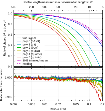
The effectiveness of correcting the estimated by dividing with is evident. There are small residual differences even for the true signal, stemming from it being still finite, albeit very long, and thus random. Furthermore, the corrections start to cease being perfect for large . This is an effect of discretization.
Finally we note that the leading-order approximations (31) and (34) would not be changed by putting . In fact, since these terms are exponentially small in , this change does not influence any terms in series expansions in powers of for . The same approximation (and conclusion) follows from writing
| (35) |
in (21) and disregarding the second term, exponentially small compared to the first. The integral to infinity is generally much easier to evaluate, in particular in higher dimensions, and allows obtaining formulae for small [9].
3.4 Two-dimensional polynomial background
Two-dimensional orthonormal polynomials on can be constructed as separable, i.e. products of 1D polynomials (26)
| (36) |
Clearly then
| (37) |
and other 2D expressions, such as the integrals in (22), reduce to products of 1D expressions in a similar manner.
Usually the total degree of the polynomial is limited, leading to the following basis function sets (on square ):
-
•
constant ,
-
•
plane levelling, adding and ,
-
•
quadratic levelling, adding , and ,
-
•
cubic levelling, adding the four cubic basis functions,
-
•
etc.
Evaluation of the integral (22) then results in functions for 2D polynomial levelling.
However, there are other common choices for the set of polynomials. Frequently the maximum degrees of and are chosen separately, in particular when the image is not square or there are other reasons for using different levelling along the two axes. Enumeration of all reasonable two-dimensional is not feasible. Therefore, we instead describe a procedure for their construction:
-
1.
Take the set of 2D terms which define the polynomial background.
-
2.
For each term look up the corresponding and in table 1.
-
3.
For each term calculate polynomials and according to (27). Multiply the two polynomials.
-
4.
Sum the results for all terms.
This procedure is applicable if the set of degrees is convex, i.e. if under the following condition: If is included then are included too for all degrees and . Otherwise the Legendre polynomials would not have the same linear span as the monomials. This condition is satisfied by all practical background subtraction methods in AFM.
For Gaussian ACF (28) and limited total degree we obtain the leading terms for small
| (38) |
The second term in the brackets must be small compared to 1 for the leading-order approximation to be valid. Unfortunately, Gaussian ACF may be the only interesting case for which has a closed form expression because Gaussian is the only separable radially symmetric function.
-
0 1 2 3 4 5
For other radially symmetric ACF , i.e. isotropic roughness, we can obtain leading-order terms using (35) and transformation to polar coordinates and . As in one dimension, this results in an asymptotic series for if decays faster than any power . The integral then becomes
| (39) |
where the inner integral expressing is elementary because is a polynomial. Polynomials are listed in table 5 for degrees up to 5 for reference.
The outer integral is of the same type as in the 1D case for the same . For exponential ACF (28) this results in
| (40) |
3.5 Intermediate Gaussian–exponential ACF
Gaussian and exponential ACF belong to a one-parametric class of simple classical ACF models, usually called power-exponential or intermediate Gaussian–exponential ACF [33, 9]. The parameter is the power in the exponent:
| (41) |
Clearly and 2 correspond to exponential and Gaussian (28), and represents a class of randomly rough surfaces transitioning smoothly between them. The corresponding spectral densities do not have closed forms and the ACF form is not physically motivated. Nevertheless, it can match reasonably many real surfaces. In this this context the main advantage of this model is that bias expressions (35) and (39) have simple closed forms.
In order to derive asymptotic series in powers of for (i.e. disregarding exponentially small terms), we need to evaluate the integrals to infinity (35) and (39). They have both the same form
| (42) |
where is a polynomial–either in 1D (table 2) or in 2D (table 5)—and is given by (41). Writing the polynomial
| (43) |
we need to evaluate
| (44) |
which can be easily transformed () to
| (45) |
where denotes the gamma function.
Coefficients are given by the basis functions. For 1D polynomials the leading coefficients are
| (46) |
whereas for 2D polynomials
| (47) | |||
| (48) | |||
| (49) | |||
| (50) |
Substituting them into (45) gives leading order terms for 1D bias
| (51) |
and for 2D bias
| (52) |
These expressions can be used to reproduce (31) and (38) with , (34) and (40) with , and similar expressions for ACF of the form (41) for other .
3.6 Reference plots
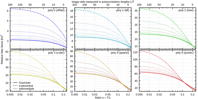
Results of the preceding sections can be summarized in graphical form for a quick estimation of the bias in common measurement scenarios. It always begins with estimating the ratio , usually by knowing exactly and estimating .

For 1D processing figure 3 can be then used. It summarises the relative bias for Gaussian and exponential ACF, as well as intermediate ACF types with step of 0.2. It was plotted using exact integrals and is, therefore, valid even for large .
After choosing the corresponding curve according to polynomial degree and ACF type, one multiplies the value from figure 3 by to obtain the relative bias , and possibly further by for an absolute number.
An example of bias estimation using figure 3:
-
1.
We measured a AFM image and removed bow from each scan line.
-
2.
This means 1D processing, and polynomial degree of 2.
-
3.
We estimate correlation length as . The surface is locally smooth and roughness can be assumed not far from Gaussian.
-
4.
This gives , so on the full green curve we read .
-
5.
We estimate the bias of as .
The difference between Gaussian and exponential ACF is relatively small in 1D. The ratio for corresponds to the ratio of leading terms in (31) and (34). However, the difference actually decreases for larger thanks to the higher order terms (up to a cross-over point). Furthermore, the curves for a large range of powers remain quite close to Gaussian, even up to . Assuming a Gaussian ACF can, therefore, often give a reasonable estimate even if the ACF deviates from Gaussian.
Independently on the ACF type, the bias is quite high. Even for in the range of hundreds, it remains at least a few percent and it becomes much larger as decreases. It is not difficult to find realistic scenarios in which it reaches 20, 30 or even 40 %.
For 2D processing figure 4 can be used instead of figure 3. Although even for most image data processing the bias is dominated by 1D processing, a quick check of the 2D levelling contribution is still useful. The factors in figure 4 must be multiplied by (instead of ) since the leading term is proportional to in 2D. Otherwise the estimation procedure remain unchanged. Note that the polynomial degree in figure 4 correspond to the limited total degree. For other combination of and degrees one can utilize the observation that the leading term is proportional to the number of coefficients fitted.
The dependence on ACF shape is evidently stronger in 2D than it is in 1D. The ratio of leading terms is now 2 between exponential and Gaussian ACF. It still holds that the curves remain closer to Gaussian ACF for relative large powers . However, due to larger absolute differences, it is no longer reasonable to universally assume Gaussian ACF.
Also, the proportionality to means that the bias remains quite low up to around 0.05 (depending on polynomial degree). But once it becomes non-negligible, it grows rapidly. Therefore, keeping sufficiently large can be a feasible strategy for avoiding bias caused by 2D data processing—in contrast to 1D processing.
3.7 Spatial frequency filtering
Spatial frequency filtering removes (or suppresses) specific spatial frequencies. It is usually done in the frequency space utilizing the Fourier transform. It yields the best representation of the data using and sines and cosines in the least-squares sense and thus lies within the same framework. The basis functions are orthonormal and come in pairs
| (53) |
Therefore, for one particular spatial frequency (22) becomes
| (54) |
which evaluates to
| (55) |
Substituting this expression to (21) leads to bias
| (56) |
where is normalized ACF. Since ACF is the Fourier transform of spectral density of spatial frequencies, removing one frequency from the spectral density corresponds to removing one frequency component from the ACF.
However, expression (56) is not exactly the -th Fourier coefficient of ACF. It would be if was non-zero only when , allowing replacing the integral with
| (57) |
This corresponds to the case . The difference between (56) and spectral density at frequency is due to the limited length and for background removal, i.e. small frequencies , it is of order in 1D.
Since the data spectral density usually has a maximum at the zero frequency and then monotonically decreases, filtering of low frequencies is the background removal which most efficiently reduces because it always takes the largest remaining component. Nevertheless, for the lowest frequencies the result is quite similar to the subtraction of polynomials.
3.8 Median levelling
Instead of the mean value, other quantities are sometimes subtracted during levelling, for instance median or trimmed mean. The motivation is that they are less sensitive to outliers. These operations are non-linear and thus outside the framework developed above.
For 1D data they are also inconsistent with ‘mean value of is zero’. Furthermore, if we subtracted the mean value afterwards it would nullify the effect of subtracting something else first. However, they can be meaningful for 2D data. When correcting misaligned scan lines, each is levelled individually using the non-linear operation. This effect survives subsequent subtraction of mean value from the entire image—which, in fact, then frequently has very little effect.
The estimated is again expressed by (5) if we replace by the subtracted quantity, which will be denoted (for median). It is useful to write as both and are location estimates, so their difference is presumably small. This gives expected value
| (58) |
as all mixed terms cancel. Therefore, the negative bias is always slightly reduced compared to mean value subtraction and the expected difference is simply . Numerical results confirm this conclusion. Asymptotic expressions for are known for many distributions in the case of uncorrelated data. For instance for median and Gaussian distribution , where is the number of data values. More generally, tends to a constant for if the probability density decays sufficiently fast.
For correlated data again has to be replaced with . Numerical calculations give
| (59) |
as a reasonable approximations in most cases, with and for 1D and Gaussian ACF, and for 2D and Gaussian ACF, and and for 2D and exponential ACF. The exception is exponential ACF in 1D for which
| (60) |
with and is more suitable for covering a wider range. In both formulae corresponds to the limit and we can put for a rough estimate.
Considering the small differences between biases for mean and median levelling, detailed analysis of trimmed means is unnecessary. The bias lies between values for mean and median—and this is sufficient for its estimation.
4 Bias of other quantities
So far, we only considered the bias of . It has a linear definition, making it suitable for averaging, and it often arises naturally in physical calculations, for instance in optics. Replacing with corrects its bias. However, there are many other quantities characterizing the extent or variance of heights of rough surfaces. We will consider unsquared and average roughness, denoted Ra (whether in 1D or 2D). Finally, we will introduce a single symbol for to avoid confusing notation: .
It might seem that if we correct by dividing by then corrected should simply use . Unfortunately, this is only true in the limit . For finite correcting by does not result in an unbiased estimate. The reason is that has non-zero dispersion (proportional to [9]) and square root is a non-linear transformation. Since square root is concave, the Jensen’s inequality [34, 21] states that underestimates when itself is unbiased.
The Taylor expansion of around gives an expression in term of -th central moments [35]
| (61) |
Although the values entering (6) are correlated, the law of large numbers still means will tend to the normal distribution (the dispersion of heights is obviously finite). Therefore, we can estimate and , which hold for central moments of the normal distribution. However, the variance depends on the dimension, ACF type, levelling method and is, of course, a function of . The leading term is [9]
| (62) |
where is a constant for given ACF. In general, (62) is again a series in . Together with (61), this again give a series expression
| (63) |
for the biased mean value of . The bias is again negative and can be corrected by dividing by the term in parentheses.
One consequence of relation (62) which needs to be emphasized is that there is a difference between averaging independent profiles and correlated image rows. The bias is the same in both cases if row-wise processing is applied. However, the variance of is reduced by factor for independent scan lines, whereas for the image it is reduced only by , where is the vertical sampling step. So both the variance and the bias originating from (62) are larger for correlated image rows.
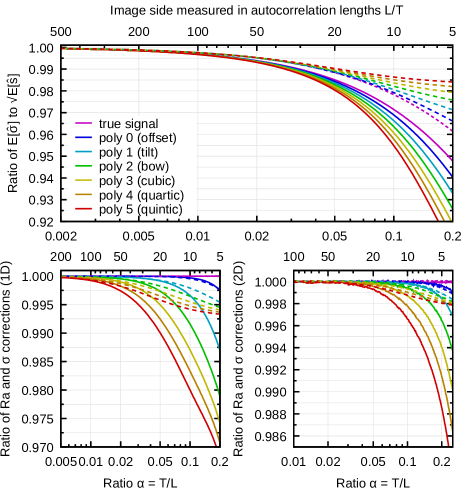
Nevertheless, the bias following from variance is largest for single profiles, where no averaging reduces it. Its magnitude is illustrated in figure 5 for this 1D case and Gaussian and exponential ACF. Even in this case it does not exceed 1–2 % for reasonable ratios, although it is somewhat higher for the Gaussian ACF. For other cases the bias is negligible since it is smaller by at least another order of magnitude.
Concerning Ra, the ratio Ra/ is a constant for any particular distribution of heights. Therefore, in the limit the correction factor for Ra—or any other quantity characterizing linearly the variance of heights—is the same as for . Of course, the main point of this work is that cannot be considered zero. The distribution of heights changes somewhat by levelling, so we must ask how much the correction factors change with increasing .
The results of numerical calculations are plotted in figure 5. Fortunately, the ratios of correction factors for Rq and Ra are close to unity, even though they are much larger for Gaussian ACF than for exponential. In 2D the effect can be probably safely disregarded, in 1D it may be useful to consider it, depending on the ACF form.
5 Experimental example
A realistic example illustrating the impact of profile length on measured roughness quantities is shown in 6. It was obtained by measuring a set of long profiles of a surface roughness standard from Edmund Optics based on electroformed nickel plates representing different surface finishes. Measurements were done using the Nanomeasuring and Nanopositioning Machine NMM1 [36] from SIOS company. Combined with a custom built AFM head (used in contact mode here with PPP-CONTR cantilevers), the instrument can be used for measurements over even a centimetre areas. The measured profiles were approximately 1.2 mm long, approximately 1000 longer than the estimated correlation length of 12. Data corresponding to shorter evaluation lengths were then obtained by cutting short segments from these profiles.
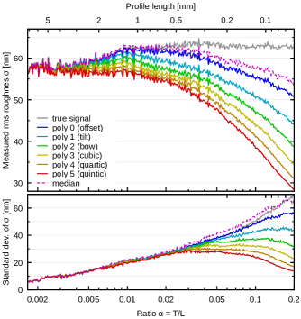
The dependency of measured mean square roughness on is plotted in figure 6 for each polynomial degree from 0 to 5 and for illustration for median levelling as well (even though it does not satisfy the zero-mean assumption). Overall, the dependencies resemble the theoretical curves, as illustrated for instance in figure 2 for Gaussian ACF. The decrease of for smallest is an artefact caused by levelling of the long base profile. The longer profiles cut from it were already of comparable lengths; a longer base profile would be necessary for stable result.
Figure 6 also illustrates the standard deviation of measured as a function of . According to the asymptotic estimates [9] it should not depend on the levelling for small . This is confirmed as up to the curves are indistinguishable. Considering contributions to measurement uncertainty, this random part predominates, at least for a single evaluation. However, it can be reduced by evaluating roughness multiple times, which is anyway recommended. In contrast, the bias is unaffected by repeated measurement because it is inherently tied to .
6 Conclusion
Bias caused by limited measurement area is a universal and mostly unavoidable effect skewing measured roughness values. While the effect itself is well known (mostly for the case of mean value subtraction), it is not commonly taken into account, neither in roughness measurement standards, nor in practice. It is made worse by the use of aggressive levelling in atomic force microscopy data processing as the subtraction of higher order polynomials increases the bias. And it is further exacerbated by levelling of topographical images scan line by scan line. While this step is often necessary, it turns 2D data processing to 1D, at least from the bias standpoint—we are then effectively analysing profiles of the length of one scan line.
We developed a framework for the calculation of the bias using known data autocorrelation function (ACF) for levelling by subtraction of any linearly-fitted background. Beside exact results, it allowed providing expressions in the form of series for 1D and 2D data polynomial levelling and common ACF types. We noted that in 1D processing, the dependency on ACF type is relatively weak and it seems to be possible to simply assume Gaussian ACF if the surface is close to locally smooth. Some common levelling methods are non-linear. Of these, we examined median levelling and found that it is similar to mean value subtraction as its effect is essentially the removal of one degree of freedom. Finally, the translation of results for squared mean square roughness to other quantities was discussed.
For an easy rough estimation of the bias, two sets of reference plots were provided for both 1D and 2D data processing (figures 3 and 4), covering a range of ACFs from Gaussian to exponential, including several intermediate types, and levelling polynomial degrees from 0 to 5. After estimating the ratio of correlation length to scan line length, they allow obtaining the relative negative bias of . For Ra, Sa, Rq or Sq the bias is approximately half this value.
Acknowledgements
This work was supported by the EURAMET joint research project ”Six degrees of freedom” funded from the European Union’s Seventh Framework Programme, ERA-NET Plus, under Grant Agreement No. 217257, and by the Ministry of Education, Youth and Sports of the Czech Republic under the project CEITEC 2020 (LQ1601).
References
References
- [1] Xiaoke He, Weixuan Jiao, Chuan Wang, and Weidong Cao. Influence of surface roughness on the pump performance based on computational fluid dynamics. IEEE Access, 7:105331–105341, 2019.
- [2] Pedram Alipour, Davood Toghraie, Arash Karimipour, and Mehdi Hajian. Modeling different structures in perturbed Poiseuille flow in a nanochannel by using of molecular dynamics simulation: Study the equilibrium. Physica A: Statistical Mechanics and its Applications, 515:13–30, 2019.
- [3] T Pravinraj and R Patrikar. Modeling and characterization of surface roughness effect on fluid flow in a polydimethylsiloxane microchannel using a fractal based lattice boltzmann method. AIP Advances, 8:065112, 2018.
- [4] Marcus Trost and Sven Schröder. Roughness and scatter in optical coatings. In Miloslav Ohlídal and Olaf Stenzel, editors, Optical Characterization of Thin Solid Films, volume 64 of Springer Series in Surface Sciences, pages 377–405. Springer, Cham, 2018.
- [5] G Macias, M Alba, L F Marsal, and A Mihi. Surface roughness boosts the sers performance of imprinted plasmonic architectures. Journal of Materials Chemistry C, 4:3970–3975, 2016.
- [6] F Tan, T Li, N Wang, S K Lai, C Chung Tsoi, W Yu, and X Zhang. Rough gold films as broadband absorbers for plasmonic enhancement of tio2 photocurrent over 400–800 nm. Scientific Reports, 6:33049, 2016.
- [7] Yanjun Shen, Yongzhi Wang, Yang Yang, Qiang Sun, Tao Luo, and Huan Zhang. Influence of surface roughness and hydrophilicity on bonding strength of concrete-rock interface. Construction and Building Materials, 213:156–166, 2019.
- [8] Gülistan Koçer, Jeroen ter Schiphorst, Matthew Hendrikx, Hailu G. Kassa, Philippe Leclère, Albertus P. H. J. Schenning, and Pascal Jonkheijm. Light‐responsive hierarchically structured liquid crystal polymer networks for harnessing cell adhesion and migration. Advanced Materials, 29:1606407, 2017.
- [9] Yiping Zhao, Gwo-Ching Wang, and Toh-Ming Lu. Characterization of Amorphous and Crystalline Rough Surface – Principles and Applications, volume 37 of Experimental Methods in the Physical Sciences. Academic Press, San Diego, 2000.
- [10] ISO 4287:1997. Geometrical product specification (GPS). surface texture. profile method. terms, definitions and surface texture parameters, 1997.
- [11] ASME B46.1 (2009). Surface texture (surface roughness, waviness, lay). Am. Soc. Mech. Eng.
- [12] ISO 25178:2012. Geometric product specifications (GPS) – surface texture: Areal, 2012.
- [13] ISO 19606:2017. Fine ceramics (advanced ceramics, advanced technical ceramics) — test method for surface roughness of fine ceramic films by atomic force microscopy, 2017.
- [14] A.-L. Barabási and H. E. Stanley. Fractal concepts in surface growth. Cambridge University Press, New York, 1995.
- [15] David Nečas and Ivan Ohlídal. Consolidated series for efficient calculation of the reflection and transmission in rough multilayers. Opt. Express, 22:4499–4515, 2014.
- [16] Martin Čermák, Jiří Vohánka, Ivan Ohlídal, and Daniel Franta. Optical quantities of multi-layer systems with randomly rough boundaries calculated using the exact approach of the Rayleigh–Rice theory. J. Mod. Opt., 65:1720–1736, 2018.
- [17] Petr Klapetek. Quantitative Data Processing in Scanning Probe Microscopy. Elsevier, 2nd edition, 2018.
- [18] Christopher A. Brown, Hans N. Hansen, Xiang Jane Jiang, François Blateyron, Johan Berglund, Nicola Senin, Tomasz Bartkowiak, Barnali Dixon, Gaëtan Le Goïc, Yann Quinsat, W. James Stemp, Mary Kathryn Thompson, Peter S. Ungar, and E. HassanZahouani. Multiscale analyses and characterizations of surface topographies. CIRP Annals, 67:839–862, 2018.
- [19] ISO 25178-2:2012. Geometrical product specifications (GPS) – surface texture: Areal – part 2: Terms, definitions and surface texture parameters, 2012.
- [20] Theodore W. Anderson. The Statistical Analysis of Time Series. Wiley series in probability and mathematical statistics. John Wiley & Sons, New York, 1971.
- [21] Venkatarama Krishnan and Kavitha Chandra. Probability and Random Processes. Wiley, 2nd edition, 2015.
- [22] George E. P. Box, Gwilym M. Jenkins, Gregory C. Reinsel, and Greta M. Ljung. Time Series Analysis: Forecasting and Control. Wiley, 5th edition, 2015.
- [23] David Nečas and Petr Klapetek. One-dimensional autocorrelation and power spectrum density functions of irregular regions. Ultramicroscopy, 124:13–19, 2013.
- [24] Daniel Zwilinger. Handbook of Integration. Jones and Bartlett Publishers, London, 1992.
- [25] K. Schouterden, B. M. Lairson, and M. H. Azarian. Optimal filtering of scanning probe microscope images for wear analysis of smooth surfaces. J. Vac. Sci. Technol. B, 14:3445–3451, 1998.
- [26] Daniel P. Fogarty, Amanda L. Deering, Song Guo, Zhongqing Wei, Natalie A. Kautz, and S. Alex Kandela. Minimizing image-processing artifacts in scanning tunneling microscopy using linear-regression fitting. Rev. Sci. Instrum., 77:126104, 2006.
- [27] Alejandro Gimeno, Pablo Ares, Ignacio Horcas, Adriana Gil, José M. Gómez-Rodríguez, Jaime Colchero, and Julio Gómez-Herrero. ‘flatten plus’: a recent implementation in WSxM for biological research. Bioinformatics, 31:2918–2920, 2015.
- [28] Ph. Dumas, B. Bouffakhreddine, C. Amra, O. Vatel, E. Andre, G. Galindo, and F. Salvan. Quantitative microroughness analysis down to the nanometer scale. Europhysics Letters, 22:717–722, 1993.
- [29] Jaechoul Lee and Robert Lund. Revisiting simple linear regression with autocorrelated errors. Biometrika, 91:240–245, 2004.
- [30] Ronald N. Bracewell. The Fourier Transform & Its Applications. McGraw-Hill, Singapore, 1999.
- [31] Milton Abramowitz and Irene A. Stegun. Handbook of mathematical functions with Formulas, Graphs, and Mathematical Tables. National Bureau of Standards, Washington, 1964.
- [32] Maxima, a computer algebra system, version 5.42.1. http://maxima.sourceforge.net/, 2019.
- [33] Giorgio Franceschetti and Daniele Riccio. Scattering, Natural Surfaces, and Fractals. Academic Press, London, 2007.
- [34] J. L. W. V. Jensen. Sur les fonctions convexes et les inégalités entre les valeurs moyennes. Acta Mathematica, 30:175–193, 1906. in French.
- [35] S. M. Kendall and A. Stuart. The Advanced Theory of Statistics, Vol. 1 Distribution Theory. C. Griffin and Co., London, 1977.
- [36] E. Manske, T. Hausotte, R. Mastylo, T. Machleidt, K.-H. Franke, and G. Jäger. New applications of the nanopositioning and nanomeasuring machine by using advanced tactile and non-tactile probes. Meas. Sci. Technol., 18:520, 2007.