Wolf-Rayet galaxies in SDSS-IV MaNGA. I. Catalog construction and sample properties

Abstract

Wolf-Rayet (WR) galaxies are a rare population of galaxies that host living high-mass stars during their WR phase (i.e. WR stars), and are thus expected to provide interesting constraints on the stellar Initial Mass Function, massive star formation, stellar evolution models, etc. Spatially resolved spectroscopy should in principle provide a more efficient way of identifying WR galaxies than single-fiber surveys of galactic centers such as SDSS-I & II, as WR stars should be more preferentially found in discs. Using Integral Field Unit data from the ongoing SDSS-IV MaNGA survey, we have performed a thorough search for WR galaxies in a two-step method. We first identify H II regions in each datacube and carry out full spectral fitting to the stacked spectra. We then visually inspect the residual spectrum of each H II region and identify WR regions that present a significant “blue bump” at $4600-4750$ Å. The resulting WR catalog includes 267 WR regions of $\sim$500 pc (radius) sizes, distributed in 90 galaxies from the current sample of MaNGA (MaNGA Product Launch 7). We find WR regions are exclusively found in galaxies that show bluest colors and highest star formation rates for their mass. Most WR galaxies have late-type morphologies and show relatively large asymmetry in their images, implying that WR regions are more preferentially found in interacting/merging galaxies. We estimate the stellar mass function of WR galaxies, and the mass-dependent detection rate. The detection rate of WR galaxies is typically $\sim$2%, with weak dependence on stellar mass. This detection rate is about 40 times higher than previous studies with SDSS single fiber data, and by a factor of 2 lower than the CALIFA-based WR catalog. We make comparisons with SDSS and CALIFA studies, and conclude that different detection rates of different studies can be explained mainly by three factors: spatial coverage, spectral signal-to-noise ratio, and redshift ranges of the parent sample. We tabulate the WR galaxy properties for future studies.

1 Introduction

Wolf-Rayet (WR) galaxies are a rare population of galaxies showing significant feature of WR stars, which were initially identified by Wolf & Rayet (1867) and are believed to evolve from O-type stars with an initial mass of 25 $M_{\odot}$ or larger. WR stars manifest their existence by presenting a series of broad emission lines in the optical wavelength range such as the broad He II line at 4686 Å, produced by their dense stellar winds (Crowther, 2007). Due to their small number at birth and short lifetime, WR stars are expected to be a small fraction of the stellar population in a galaxy, and therefore WR galaxies must be a rare population as well.

The Milky Way is expected to have thousands of WR stars, and several hundred have been detected (van der Hucht, 2001) and is presented in a continuously maintained online catalog . Extra-galactic WR features were firstly identified by Allen et al. (1976) in the galaxy He 2-10, which was later termed “Wolf-Rayet galaxy” by Osterbrock & Cohen (1982). By the end of the last century, a total of only 139 WR galaxies beyond the Local Group were reported (Schaerer et al., 1999). Most cases were fortuitous discoveries, and only a few resulted from intentional systematic searches through spectroscopy (Kunth & Joubert, 1985, e.g.) or narrow-band imaging (Drissen et al., 1993, e.g.). Thanks to the large spectroscopic galaxy sample from the Sloan Digital Sky Survey (SDSS; York et al., 2000), the detection and study of WR galaxies have advanced dramatically. Zhang et al. (2007) published the first SDSS-based WR galaxy catalog with 174 WR galaxies from the SDSS Data Release 3 (DR3). Two more catalogs based on later data releases consist of 570 (Brinchmann et al., 2008, from SDSS DR6) and 271 WR galaxies (Agienko et al., 2013, from blue compact dwarf galaxies in SDSS DR7), respectively. Despite different selection procedures and criteria adopted in these studies, the fraction of WR galaxies in the SDSS samples has consistently been very small, at the order of $\sim$0.05%.

The low detection rate of WR galaxies should be partially attributed to the fact that SDSS spectroscopy is limited to the central 1-2 kpc of galaxies. It is natural to expect higher detection rates in outer regions of galaxies considering that star formation occurs more widely in galactic discs than in their centers. In addition, the actural area covered by the three-arcsec fiber of SDSS can substantially vary over the (though narrow) redshift range of the survey, thus diluting WR signatures from the center of distant galaxies due to inclusion of non-WR area at large radii, while missing off-center WR signatures in nearby galaxies due to the limited aperture of the fiber. This aperture bias can be largely overcome using the technique of integral field unit (IFU) which obtains spatially resolved spectroscopy out to large radii in/around a galaxy. Indeed, detection of WR galaxies has advanced in recent years thanks to the recent/ongoing IFU surveys, allowing searches for WR regions across the whole galaxy. Miralles-Caballero et al. (2016) has recently applied an automated searching procedure to the IFU data from the Calar Alto Legacy Integral Field Area survey (CALIFA; Sánchez et al., 2012a), identifying 44 WR regions in 25 galaxies out of a total of 558 galaxies at $0.005<z<0.03$. About one third of the WR regions are located within $\sim$1kpc from the center of their host galaxies. Both the fraction of WR galaxies ($\sim 5\%$) and the fraction of central WR regions ($\sim 1/3$) in the CALIFA sample are much higher than the WR galaxy fraction ($\sim 0.05\%$) in the SDSS sample, which cannot be simply explained by the different sample selections of the two surveys or the limited spatial coverage of the SDSS single-fiber spectroscopy.

WR galaxies are interesting not only for their rareness. They have been used as unique probes of massive star evolution, ionization origin of ions (e.g. He II) and dense stellar winds in galaxies, thus providing important constraints on stellar population synthesis models of galaxies. For instance, by analyzing long-slit spectra of 39 WR galaxies, Guseva et al. (2000) found the relative number of WR stars to O stars to decrease with decreasing metallicity, in agreement with evolutional stellar population synthesis models. In addition, it was found that galaxies with He II $\lambda$4686 emission do not always present WR features, indicating that WR stars are not the only ionizing source of He II. This finding was confirmed and discussed in Brinchmann et al. (2008) and Shirazi & Brinchmann (2012). With the first SDSS-based WR catalog, Zhang et al. (2007) performed a comparison of the WR emission of galaxies with theoretical predictions from evolutionary synthesis models following Guseva et al. (2000), finding that a metallicity-dependent variation of the slope of stellar Initial Mass Function (IMF) appears to be necessary in order for the models to agree with the data. Using a larger sample of WR galaxies selected from a later SDSS data release, Brinchmann et al. (2008) found the likelihood of galaxies showing WR features increases with increasing metallicity, although the WR galaxies present a wide range in morphology. In particular, WR galaxies showed an elevated nitrogen-to-oxrygen (N/O) ratio relative to non-WR galaxies, implying a rapid enrichment of the interstellar medium (ISM) from WR winds. IFU data available in recent years have been used to further study the N/O ratio of WR galaxies as supporting evidence for metal pollution from WR winds (e.g. Pérez-Montero et al., 2013; Miralles-Caballero et al., 2014). The WR catalog constructed from CALIFA by Miralles-Caballero et al. (2016) has revealed the similarity between WR galaxies and Gamma-Ray Burst host galaxies, as well as the importance of binary stellar evolution for modeling the WR emission at low metallicity.

In this paper we present a thorough search of WR galaxies in the ongoing Mapping Nearby Galaxies at Apache Point Observatory (MaNGA; Bundy et al., 2015) survey. As one of the three major experiments of the fourth generation of the Sloan Digital Sky Survey (SDSS-IV; Blanton et al., 2017), MaNGA is obtaining IFU data for 10,000 galaxies at $0.01<z<0.15$ selected from the SDSS galaxy sample. We identify our WR galaxies in a two-step method, in which we firstly identify H II regions according to the two-dimensional map of H$\alpha$ surface brigthness of each galaxy, and then visually inspect the integrated spectrum of each H II region obtained by stacking the original spectra of all spaxels falling in the region. Following previous studies, we classify an H II region to be a WR region if it presents a significant blue bump over the wavelength range $4600-4750$ Å. This bump is a blend of broad emission lines from He II, N III, N V, C III and C IV in stellar winds of WR stars. The ratios among these broad lines vary with the number ratio of carbon-rich WR stars (namely WC star) and nitrogen-rich WR stars (namely WN star). Another signature of WR galaxies is a red bump around 5800 Å from broad emission lines of C III and C IV. Normally the red bump is much fainter than the blue bump and other WR features are even fainter than the red bump. Therefore, most searches for WR galaxies including this work have made use of the blue bump signature. Out of the 4621 galaxies from MaNGA Product Lauch 7 (MPL-7), we have constructed a catalog of 90 WR galaxies including a total of 267 WR regions. In this paper we present the identification process of these WR regions, as well as the global properties of the sample. In a parallel paper, we study the spatial distribution of the WR regions and dependence on galaxy properties.

The rest of the paper is arranged as follows. Section § 2 presents a description of the SDSS-IV MaNGA data and our searching procedure of WR galaxies. Section § 3 presents the catalog and basic properties of our WR galaxies including the mass-dependent detection rate and scaling correlations of mass, color and metallicity. In § 4 we discuss our results and connect them with the litereatue. We summarize in § 5.

2 Data and selection procedure

2.1 Overview of the MaNGA survey

As one of the three core surveys of the SDSS-IV project (Blanton et al., 2017), MaNGA aims to obtain integral-field spectroscopy for an unprecedented sample of 10,000 nearby galaxies with $0.01<z<0.15$ over a six-year survey period from July 2014 through June 2020 (Bundy et al., 2015). MaNGA utilizes the two dual-channel BOSS spectrographs at the 2.5-meter Sloan Telescope (Gunn et al., 2006; Smee et al., 2013), covering a wavelengh range of 3622-10354 Å with a spectral resolution R$\sim$2000, and reaching a target $r$-band signal-to-noise $S/N=4-8$ (Å^-1 per $2^{\prime\prime}$-fiber) at 1-2 $R_{e}$ (effective radius) with a typical exposure time of 3 hours. MaNGA uses 29 fiber bundles to obtain the IFU data, including 12 seven-fiber mini-bundles for flux calibration and 17 science bundles with five different field of views (FoVs) ranging from 12^′′ to 32^′′, covered by different numbers of fibers ranging from 19 up to 127. MaNGA instrumentation is described in detail in Drory et al. (2015).

MaNGA targets are selected from the NASA Sloan Atlas v1_0_1 (NSA), a catalog constructed by Blanton et al. (2011) including physical parameters for $\sim$640,000 galaxies from GALEX, SDSS and 2MASS. Wake et al. (2017) describe the MaNGA sample selection, which was designed and optimized so as to simultaneously optimize the IFU size distribution, the IFU allocation strategy and the number density of targets. The sample consists of three subsamples: the Primary and Secondary samples having a flat distribution of the $K$-corrected $i$-band absolute magnitude ($M_{i}$) and covering out to 1.5 and 2.5$R_{e}$ respectively. The third subsample, the Color-Enhanced sample selects galaxies on the plane of $NUV-i$ color versus $M_{i}$ that are not well sampled by the Primary sample. Overall, the MaNGA sample covers the stellar mass range $5\times 10^{8}M_{\odot}h^{-2}<M_{\ast}<3\times 10^{11}M_{\odot}h^{-2}$ with a median redshift of $z\sim 0.03$.

MaNGA raw data are reduced with the Data Reduction Pipeline (DRP; Law et al., 2016). The DRP product for each galaxy is provided in the form of a datacube with a spaxel size of 0.5″, and the effective spatial resolution of the datacubes can be described by a Gaussian with a full width at half maximum (FWHM) $\sim$2.5″. Flux calibration, survey strategy and data quality tests are described in detail in Yan et al. (2016a, b). For more than 80% of the wavelength range of MaNGA, the absolute flux calibration is better than 5%.

In this work we make use of MaNGA Product Launch-7 (MPL-7), which contains 4688 datacubes for 4621 unique galaxies. The MPL-7 is identical to the MaNGA data included in the SDSS data release 15 (DR15; Aguado et al., 2019). In addition to the reduced datacubes from the DRP, the DR15 also provides products of the Data Analysis Pipeline (DAP) developed by MaNGA collaboration (Westfall et al., 2019). The DAP performs full spectral fitting to the DRP datacubes using the MILES-HC stellar spectral library (Falcón-Barroso et al., 2011), producing measurements of kinematic parameters, emission line profiles, stellar indicies, etc. We use DRP spectra and DAP products as a starting point in our precedure of searching for WR regions, as described in subsection 2.2 below. We also take advantage of the data visualization and access tool of MaNGA Marvin developed by Cherinka et al. (2019), which includes an online part enabling individual galaxies to be examined quickly and conveniently.

2.2 Overview of WR Searching procedure

We search for WR galaxie in a two-step scheme. For each galaxy in MaNGA MPL-7, we firstly identify H II regions using the two-dimensional map of H$\alpha$ surface brightness provided by the DAP. For each H II region, we stack the DRP spectra of all spaxels falling in the region. Next, we perform full spectral fitting to all the stacked spectra, and we visually inspect the residual spectra to identify WR regions. An H II region is identified to be a WR region if it presents a significant blue bump in the residual spectrum, and a galaxy is identified to be a WR galaxy if it contains one or more WR regions. In the following subsections we describe our searching procedure in detail. We focus on the blue bump WR feature in the searching, and we will discuss other WR features such as the red bump in later sections.

2.3 Identification of H II regions

We assume that WR stars are found exclusively in star-forming regions with significant H II emission. Therefore, we start by identifying H II regions from the IFU datacube of each galaxy in MPL-7. WR features are then visually identified from the total spectrum of each H II region, obtained from stacking the original spectra of all the spaxels in the region. As we will show, the stacking significantly increases the spectral S/N, allowing those relatively weak WR feature to be more clearly seen.

We use the H II region finder called HIIexplorer developed by Sánchez et al. (2012b) for the identification of H II regions. The overall workflow of the HIIexplorer can be found in Sánchez et al. (2012b, figure 1). In short, from a given DRP datacube, spaxels with H$\alpha$ surface brightness $\Sigma H\alpha>\Sigma_{\mbox{peak}}$ are picked up in the first place as the central peak of potential H II regions. Next, for each peak spaxel, the spaxels in the vicinity are appended to the region if they meet the following three criteria: 1) H$\alpha$ surface brightness is substantially high with $\Sigma H\alpha>\Sigma_{\mbox{min}}$, 2) the ratio of its brightness to the central spaxel is substantially high with $\Sigma H\alpha/\Sigma_{cen}H\alpha>f_{\mbox{min}}$, and 3) its distance from the central spaxel does not exceed $r_{p}^{\mbox{max}}$. In practise, the algorithm starts with the highest peak with largest $\Sigma H\alpha$, and grows it by appending adjacent spaxels that meet the above requirements, before moving on to the highest peak in the remaining map. This process is repeated until every spaxel in the datacube is assigned to an H II region, or rejected.

This searching procedure guarantees every H II region is roughly centred at the peak value and is roughly round and symmetric. The minimum brightness ratio ($f_{min}$) is required so as to make each region roughly coherent, while spaxels rejected due to this requirement may still be appended to other neighbouring regions. In our work the three threshold parameters are empirically set to be $\Sigma_{\mbox{peak}}=10^{39.8}$ erg s^-1kpc^-2, $\Sigma_{\mbox{min}}=10^{39.5}$ erg s^-1kpc^-2, $f_{\mbox{min}}=0.1$, and $r_{p}^{\mbox{max}}=max$(1.5″, 500pc). The maximum distance ($r_{p}^{\mbox{max}}$) reflects the trade-off between higher S/N from stacking more spaxels in each region and stronger dilution effect to WR signatures with possible inclusion of non-WR spaxels. The typical size of H II regions ranges from a few to hundreds of parsecs (Kennicutt, 1984; Garay & Lizano, 1999; Kim & Koo, 2001; Hunt & Hirashita, 2009; Lopez et al., 2011; Anderson et al., 2019), so we cannot resolve individual H II regions due to the limited spatial resolution of MaNGA which is $\sim$2.5″, corresponding to $\sim$1.5 kpc at the median redshift of MaNGA ($z=0.03$). The maximum distance adopted above is comparable to (a half of) the MaNGA spatial resolution. Therefore, each of the H II regions identified from the MaNGA datacubes is actually a mixture of H II emission and the surrounding diffuse ionized gas (DIG). The thresholds in $\Sigma H\alpha$ ensure that the resulting H II regions are dominated by real H II emission. As Zhang et al. (2017) have shown based on a study of the DIG in MaNGA galaxies, $\Sigma H\alpha$ can be used to effectively separate H II-dominated regions from DIG-dominated regions.

Figure 1: An example of HIIexplorer applied to a MaNGA galaxy. Left panel: optical image of the galaxy with magenta hexagonal field of view of MaNGA. Right panel: H$\alpha$ surface brightness map of this galaxy. Black boundaries of H II regions are over-plotted in both panels.

In total, we have identified about 8000 H II regions distributed in 1155 galaxies, which is $\sim$25% of the MPL-7 galaxy sample. In what follows, these galaxies will be called “star-forming galaxies” and their H II regions will form the parent catalog from which the WR regions are identified. Figure 1 displays the optical image and the $\Sigma H\alpha$ map with boundaries of H II regions over-plotted for one of the star-forming galaxies, as an example. The fraction of star-forming galaxies in our work is smaller than those from previous studies. For instance, Hsieh et al. (2017) classified about half of MaNGA MPL4 galaxies as star-forming galaxies, adopting a specific star formation rate threshold. Therefore we would like to emphasize that, the fractions of star-forming galaxies and H II regions, as well as those of WR galaxies/regions to be identified below, should be taken as lower limits of the real fractions.

2.4 Spectrum stacking and full spectrum fitting

We stack the spectra within each H II region to obtain an average spectrum with high S/N. After applying DRP spectral masks, we expect very few abnormal values in spectra. Thus, we choose the “weighted mean” estimator for stacking, which is the statistically optimal choice to lower the noise. Spectra are weighted by their DRP spectral error provided at each wavelength point. We correct all spectra to the rest-frame, considering both the galaxy redshift and relative velocities of each spaxel. We choose stellar velocity from DAP rather than gas velocity traced by emission lines. This is meant for a better alignment of stellar components in H II regions, in order for a better continuum fitting in the next step. We understand this choice broadens the nebular emission lines in our stacked spectra, but the effects are minimal and insignificant for the scope of this work. This process effectively reduces the noise of our spectra, typically by about 25%. Covariance is treated following the formula in Law et al. (2016, Figure 16) for derivation of the stacked error. Basically, we first calculate the error without covariance by the standard formula in weighted mean statistics (when assuming equal input error, being a division of that error by $\sqrt{N_{spectra}}$). Then we consider the effect of covariance by multiplying that error by a factor from the formula in Law et al. (2016). The factor was obtained from a synthetic approach following Husemann et al. (2013). A mock observation of unity flux and Gaussian error was assumed and then put through data reduction, datacube resampling and spectral stacking. The standard deviation of the stacked spectrum is regarded as the real error and compared to the nominal error from error propagation without covariance, so as to obtain the correction factor.

We then perform full spectral fitting to the stacked spectrum of each H II region. Our spectral fitting code is developed from Li et al. (2005). The basic idea was to utilize a set of eigenspectra as fitting templates constructed by successive application of principal component analysis (PCA). PCA was first applied to the observed stellar library STELIB (Le Borgne et al., 2003) and some supplementary libraries. Then eigenspectra resulted from the first PCA run were used to fit a representive sample of galactic spectra selected from SDSS DR1, constituting fitting models for galactic spectra. Next, PCA is applied to the fitting models. Nine top eigenspectra from the second PCA run were obtained as the fitting templates to carry out subsequent full spectral fitting. In this work, we re-construct the fitting templates by applying PCA to the MILES single stellar population (SSP) models (Vazdekis et al., 2010, 2015), which includes 350 SSPs over 50 ages and 7 metallicity bins, assuming a Chabrier IMF Chabrier (2003). We adopt the first nine eigenspectra from the PCA as our fitting templates. For each H II region, we perform full spectral fitting using this code, iteratively masking out all significant emission lines as well as the wavelength range of the WR blue bump ($4600-4750$ Å). Details about the fitting procedure and the emission line masking scheme can be found in Li et al. (2005).

2.5 Identification of WR galaxies and WR regions

For each H II region we subtract the best-fit stellar spectrum obtained from the previous subsection from the stacked spectrum. We then estimate the significance of the blue bump $\sigma_{\mbox{bump}}$, defined as

$$\sigma_{\mbox{bump}}=\frac{\bar{f}_{\mbox{bump}}-\bar{f}_{\mbox{base}}}{f_{\mbox{rms}}},$$ (1)

where $\bar{f}_{\mbox{bump}}$ is the average flux over the bump wavelength range $4600-4750$ Å, $\bar{f}_{\mbox{base}}$ is the average of the baseline, and $f_{\mbox{rms}}$ is the root mean square of the spectrum around the baseline over two wavelength windows beside the bump: $4492-4542$ Å and $4760-4810$ Å. The baseline should in principle be a horizontal line with zero flux thus giving rise to an average of $\bar{f}_{\mbox{base}}=0$, but the actual baseline always deviates from a zero line to some degrees due to imperfect spectral fitting. In order to take into account this effect, following Brinchmann et al. (2008), we determine a local baseline with a linear fitting of the residual spectrum over 4492-4542 Å and 4760-4810 Å, and use it when estimating $\sigma_{\mbox{bump}}$ with Eqn. 1.

We consider all the H II regions with $\sigma_{\mbox{bump}}>5$, ranking them by decreasing $\sigma_{\mbox{bump}}$. We visually inspect the spectrum of each region, and classify them into four different catagories: a) a real WR region with broad emission components, b) a non-WR region with only narrow nebular emission lines, c) an active galactic nucleus (AGN) with obvious broad component in $H\alpha$ and/or $H\beta$ lines, or d) fluctuations due to noise. Figure 2 shows an example galaxy which contains a WR region at the center. The figure includes the optical image and the H$\alpha$ surface brightness map of the galaxy, location (red area inside the hexagon in row 2 column 2), full original spectrum, zoomed-in original spectrum (one narrower and one wider) and zoomed-in residual (one narrower and one wider) of the WR region. As can be seen, the spectrum of the WR region presents very strong nebular emission lines and relatively stronger emission at shorter wavelengths, indicative of strong ongoing star formation.

We have visually examined about 3200 H II regions, of which 267 are identified to certainly present WR emission. The WR regions are distributed in 90 unique galaxies. We note that one of our WR galaxies is observed twice by MaNGA. In addition, out of the remaining H II regions, we have further selected a subset of 1609 tentative WR regions whose spectra show possible WR profiles but are too weak for comfirmation at this point, 244 regions with only narrow 4686 Å He II emission and 57 suspicious quasi-WR features in red galaxies. These regions will be used for future studies.

The final catalog of WR galaxies containing their basic properties is presented in Table 1. The table’s columns are arranged in the following order: (1) sequence number of WR galaxies in this catalog; (2) MaNGA-ID for unique idendification of MaNGA galaxies, (3) plate-ifu ID for MaNGA galaxies, (4) the number of WR regions contained in each WR galaxy, (5) right ascension, (6) declination, (7) redshift from NSA catalog, (8) stellar mass from K-correction fit for Sérsic fluxes from NSA catalog (we adopt h=0.7), (9) $T$-type morphological value from Domínguez Sánchez et al. (2018), (10) NUV-r color from NSA catalog.

Figure 2: Example of visual inspection process. These combined panels are for determination of one H II region. The eight panels involve the optical image (top left) and the H$\alpha$ surface brightness map of the current galaxy, location (red area inside the hexagon in row 2 column 2), full original spectrum, zoomed-in original spectrum (one narrower and one wider) and zoomed-in residual (one narrower and one wider) of the current H II region. Spectra have been smoothed with kernel=3.

Table 1: WR galaxy catalog from MaNGA

No.	MaNGA-ID	Plate-ifu	WR region	RA	DEC	Redshift	Stellar mass	T-type	NUV-r
			number	(Degree)	(Degree)		$(log_{10}(M/M_{\odot}))$
1	12-193481	7443-12703	5	229.52558	42.74584	0.0403	10.81	5.5	2.70
2	12-192116	7495-6102	2	204.51286	26.33821	0.0261	9.05	5.8	1.14
3	1-24357	7990-3703	3	262.09935	57.54541	0.0285	9.92	3.4	1.13
4	1-37084	8078-6104	6	42.73943	0.36941	0.0442	9.64	2.9	1.19
5	1-583411	8083-12702	1	50.24541	-0.36768	0.0210	11.09	5.1	2.95
6	1-604039	8083-12705	1	50.17898	-1.10865	0.0209	10.40	5.4	2.16
7	1-604748	8131-9101	3	112.57356	39.94208	0.0500	10.09	5.3	0.88
8	1-377321	8132-3702	4	110.55615	42.18364	0.0444	9.74	4.1	2.23
9	1-43505	8135-3704	2	114.89737	37.75151	0.0305	9.82	4.7	1.78
10	1-71137	8139-12702	4	113.50057	32.21576	0.0269	9.68	2.0	1.13
11	1-389720	8150-3701	1	147.58897	31.48794	0.0017	7.88	6.2	0.73
12	1-585731	8150-6103	1	147.14825	33.42162	0.0049	10.06	4.6	2.39
13	1-38819	8156-3701	2	55.59230	-0.58320	0.0524	10.13	5.0	1.48
14	1-52677	8158-1901	1	60.85933	-5.49184	0.0384	9.45	3.2	2.40
15	1-460288	8241-6102	3	126.05963	17.33195	0.0373	10.65	4.0	2.43
16	1-46577	8243-9101	4	128.17838	52.41678	0.0433	9.89	4.2	1.74
17	1-137961	8249-3703	1	139.72047	45.72778	0.0264	10.02	-1.3	3.52
18	1-137875	8249-6102	3	137.33592	45.06551	0.0510	10.32	3.7	1.90
19	1-217300	8250-3703	5	139.73996	43.50058	0.0401	9.52	-1.6	1.54
20	1-217221	8250-6101	2	138.75315	42.02439	0.0279	10.41	4.3	2.63
21	1-585641	8252-6103	2	144.15499	48.47438	0.0259	10.57	4.0	3.15
22	1-138157	8252-9102	3	145.54153	48.01286	0.0562	10.19	3.9	1.79
23	1-255959	8256-9102	7	165.10414	43.01969	0.0375	9.89	7.0	0.75
24	1-277290	8257-12701	4	165.49582	45.22802	0.0200	10.65	5.4	2.32
25	1-277293	8257-3704	1	165.55361	45.30387	0.0202	9.00	10.0	3.86
26	1-256496	8258-3704	1	167.02504	43.89461	0.0585	10.26	3.8	1.73
27	1-282147	8261-12703	2	184.35779	46.56687	0.0235	9.55	5.9	1.41
28	1-258306	8262-3701	1	183.57898	43.53528	0.0241	9.77	3.9	2.23
29	1-589908	8262-9102	1	184.55357	44.17324	0.0245	10.44	5.2	1.99
30	1-628628	8309-3703	6	210.62359	54.27100	0.0005	8.13	-99.0	0.39
31	1-248388	8313-12702	3	240.67742	41.19726	0.0333	10.59	4.8	2.30
32	1-248352	8313-1901	2	240.28713	41.88075	0.0243	9.19	1.9	1.59
33	1-523050	8320-9101	6	206.31385	23.31651	0.0297	10.22	4.7	1.95
34	1-419028	8322-3701	3	199.06648	30.26453	0.0492	10.95	4.6	2.30
35	1-591611	8322-9101	6	199.60756	31.46795	0.0187	9.84	5.3	1.58
36	1-591379	8323-12701	1	196.37038	33.84872	0.0238	9.84	6.7	2.20
37	1-234997	8325-12702	1	209.89514	47.14768	0.0420	9.59	6.3	1.55
38	1-266045	8329-3702	1	213.49543	43.89295	0.0403	9.72	3.6	2.50
39	1-491225	8338-6102	2	172.68267	22.36354	0.0224	9.56	5.0	2.38
40	1-575796	8341-12705	2	191.49328	45.19901	0.0251	9.94	5.8	1.75
41	1-156037	8439-9102	2	143.75402	48.97674	0.0250	9.33	5.3	1.43
42	1-591580	8442-3701	1	199.21314	31.58114	0.0298	10.46	4.9	2.84
43	1-419153	8442-6102	1	199.21116	31.63067	0.0303	9.89	6.2	2.01
44	1-418242	8446-3703	1	205.58417	36.95363	0.0215	9.77	4.2	2.03
45	1-488712	8449-3703	4	169.29926	23.58566	0.0421	9.50	4.8	1.77
46	1-489814	8450-3703	2	170.44434	22.48082	0.0351	10.37	3.7	2.04
47	1-608252	8454-12703	15	154.77137	46.45411	0.0307	10.74	4.6	2.18
48	1-254342	8455-12701	4	154.73181	40.61294	0.0292	10.13	5.3	2.29
49	1-275176	8455-9101	3	157.18363	39.77859	0.0300	9.97	5.5	1.95
50	1-585744	8458-3702	9	147.56250	45.95731	0.0249	9.75	3.9	0.99
51	1-284048	8465-3701	11	195.31932	48.06019	0.0300	10.22	3.5	1.68
52	1-234092	8465-6102	1	197.54970	48.62339	0.0283	9.60	3.1	1.53
53	1-209198	8485-3702	2	233.72546	47.76180	0.0230	9.65	4.4	1.78
54	1-93305	8549-6104	1	244.40158	46.08200	0.0196	9.57	2.1	1.97
55	1-247373	8551-1902	5	234.59171	45.80194	0.0214	8.74	1.7	1.91
56	1-91019	8553-3704	1	234.97035	56.36832	0.0459	9.88	4.2	1.92
57	1-584598	8566-3704	6	115.22481	40.06964	0.0416	9.76	4.3	1.01
58	1-274368	8568-3703	1	155.69307	37.67347	0.0226	9.38	-0.6	1.90
59	1-634138	8588-12702	1	250.31305	39.29009	0.0305	10.18	4.4	2.10
60	1-136286	8606-9102	5	255.70905	36.70675	0.0328	10.05	5.1	2.08
61	1-177270	8613-12703	3	256.81775	34.82261	0.0367	9.95	3.3	1.62
62	1-178686	8623-12703	1	309.98326	0.97615	0.0522	10.43	0.1	3.63
63	1-24423	8626-12704	6	263.75522	57.05243	0.0472	8.88	3.5	0.14
64	1-379291	8712-6101	1	118.72692	53.84628	0.0349	10.84	3.5	2.68
65	1-379410	8712-6103	1	120.23007	53.67056	0.0406	9.86	2.5	2.10
66	1-71974	8713-9102	7	118.85539	39.18609	0.0332	10.66	4.8	1.33
67	1-121735	8717-3703	1	118.31817	35.57258	0.0458	9.98	1.3	2.25
68	1-44745	8719-12702	3	120.19928	46.69053	0.0194	9.80	5.6	2.03
69	1-51766	8727-3702	4	54.55405	-5.54040	0.0221	8.79	-1.2	1.48
70	1-456306	8932-3701	2	194.65534	27.17656	0.0256	9.73	4.1	1.87
71	1-456772	8934-3701	6	194.02549	27.67798	0.0165	9.23	10.0	1.58
72	1-298533	8939-6102	3	124.84327	23.74728	0.0153	9.36	5.4	1.97
73	1-164148	8941-3702	3	120.00802	27.11454	0.0426	9.75	4.2	1.84
74	1-392670	8943-12704	1	156.43286	36.02359	0.0538	10.11	3.5	1.57
75	1-279617	8945-3702	5	173.36190	47.28673	0.0456	9.85	-0.9	1.59
76	1-153038	8977-3704	2	118.77440	32.72867	0.0178	9.02	-0.3	1.67
77	1-457811	8982-9101	4	201.71365	26.59124	0.0235	10.09	10.0	2.29
78	1-386685	8987-9101	1	137.44943	27.86231	0.0204	9.25	4.9	2.00
79	1-174914	8990-6104	1	174.74526	50.00589	0.0466	10.08	4.5	1.79
80	1-314332	9024-1902	2	224.43779	33.16563	0.0300	9.70	2.6	1.65
81	1-94584	9026-3701	1	250.16267	43.34609	0.0228	9.60	-2.3	3.08
82	1-199432	9037-9101	1	234.62042	43.73320	0.0184	9.31	4.0	2.15
83	1-153938	9183-12705	2	123.10611	37.73022	0.0385	10.42	-1.9	2.30
84	1-37863	9193-12704	7	46.66491	0.06198	0.1074	10.76	-0.9	2.14
85	1-45151	9487-12702	1	122.79107	45.66357	0.0229	9.74	5.1	2.23
86	1-382712	9491-6101	1	119.17438	17.99117	0.0412	10.79	4.3	2.16
87	1-386150	9506-6102	1	133.75984	26.67535	0.0274	10.04	4.6	2.26
88	1-298835	9508-1901	2	126.08120	25.67447	0.0282	9.85	-0.2	1.72
89	1-218233	9509-3702	3	122.43975	25.88031	0.0251	9.58	4.7	1.27
90	1-594855	9883-3701	6	255.13405	32.67077	0.0325	10.37	4.3	2.30

3 Global properites of WR host galaxies

3.1 Stellar mass function of WR galaxies

Figure 3 displays the WR galaxies in the plane of stellar mass (assuming h=0.7) versus redshift. For comparison, the distribution of all galaxies in MaNGA MPL-7 is plotted as grey-scale background. Stellar masses and redshifts of all galaxies in this figure are taken from the the NSA (see § 2). MaNGA MPL-7 galaxies are distributed in two narrow bands which correspond to the Primary Sample (lower redshifts at given mass) and the Secondary Sample (higher redshifts at given mass) as described in § 2.1. Our WR catalog generally follows the distribution of parent MaNGA sample, but biased to lower redshifts with $z\lesssim 0.06$ and intermediate-to-low masses with $M_{\ast}\lesssim 10^{11}M_{\odot}$. This might be reflecting the fact that WR regions of similar sizes can be more visible if hosted by more nearby galaxies. Furthermore, at fixed redshift, the WR galaxies on average appear to be less massive than MaNGA MPL-7 galaxies, an effect that is more pronounced for the Secondary Sample. This might be attributed to selection bias, or a real trend for WR regions to be preferentially found in relatively low-mass galaxies. We will come back to this point in a later subsection.

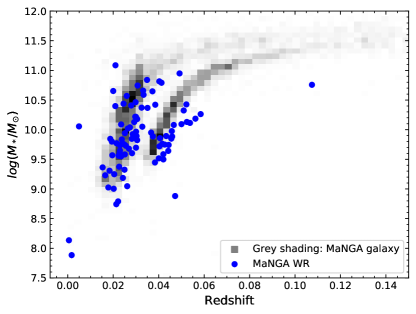
Figure 3: Distribution of WR galaxies in redshift-mass diagram. The grey shading represents the distribution of MaNGA galaxies. The blue dots are WR galaxies in our catalog.

Taking advantage of the relatively large sample size as well as the well-understood selection effects of our WR catalog, we have estimated for the first time the stellar mass function of WR galaxies, plotted as blue symbols in Figure 4. For comparison, we have estimated the stellar mass function of the general population of galaxies using MaNGA MPL-7 sample, and that of star-forming galaxies using our H II catalog. When estimating the stellar mass functions, we have corrected the effect of sample incompletness due to selections using the weights accompanying the MPL-7 release and described in detail in the Appendix of Wake et al. (2017). We only use the Primary Sample and its corresponding weights in Figure 4 for better statistics at the low mass end. The errors of the mass functions are Poisson counting error. In Table 2 we tabulate the stellar mass function estimate of our WR galaxy catalog and its ratio to the general galaxy population. Like the stellar mass function of general population, the mass function of WR galaxies can be well described by a Schechter function (Schechter, 1976). In the figure we plot the best-fit Schechter function, for which the three parameters are: amplitude $\phi_{*}$ = 0.000157 Mpc^-3, characteristic mass $log_{10}(M^{*}/M_{\odot})$ = 10.332, and the faint-end slope $\alpha$ = -0.905. The integral of this Schechter function over the mass range of $10^{9}M_{\odot}<M_{\ast}<10^{11.5}M_{\odot}$ gives an average number density of $3.47\times 10^{-4}Mpc^{-3}$ for the WR galaxies in the Local Universe. This should be regarded as a lower limit of the real number density, considering that we may have missed some weak WR regions due to the limited data quality and selection effects.

Table 2: Stellar mass function of MaNGA WR galaxies

No.	Mass	$\phi$	$\sigma(\phi)$	WR fraction	$\sigma$(fraction)
	$log_{10}(M_{*}/M_{\odot})$	Mpc-3dex-1
1	9.18-9.68	1.73E-04	6.12E-05	1.87%	0.66%
2	9.43-9.93	3.62E-04	8.31E-05	3.60%	0.83%
3	9.68-10.18	2.63E-04	6.58E-05	3.12%	0.78%
4	9.93-10.43	1.08E-04	3.24E-05	1.48%	0.45%
5	10.18-10.68	9.43E-05	3.33E-05	1.37%	0.49%
6	10.43-10.93	3.64E-05	1.29E-05	0.71%	0.25%
7	10.68-11.18	8.34E-06	4.81E-06	0.26%	0.15%
8	10.93-11.43	2.40E-06	2.40E-06	0.18%	0.18%

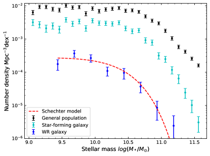
Figure 4: The stellar mass function of the WR catalog (blue dots) in comparison with the general galaxy population constructed from MaNGA Primary Sample (black dots) and star-forming galaxies defind in this work (see § 2.3; cyan dots). All samples have been applied the volume correction provided in Wake et al. (2017).

Figure 5: The detection fraction of WR galaxies in different mass bins, with respect to the general galaxy population (blue symbols) and the star-forming galaxy sample defined in this work (see § 2.3; cyan symbols). The errorbar shows Poisson counting error.

Figure 6: The NUV-r colour-mass diagram. The contours are a volume limited subsample from NSA catalog ($z<0.03$ and $log_{10}(M_{*}/M_{\odot})>9$). The grey shading is MaNGA sample corrected by galaxy weights. The blue dots are WR galaxies with S0 type WR galaxies highlighted with an additional red circle. The color and mass values are from NSA catalog. The cyan dotted lines indicate the empirical boundaries of blue cloud galaxies (lower), green valley (middle) and red sequence galaxies (upper).

As can be seen from Figure 4, the stellar mass function of WR galaxies is well determined over about two orders of magnitude in mass, from $\sim 10^{9}M_{\odot}$ up to $\sim 10^{11}M_{\odot}$. The WR galaxy sample appears to keep the same shape over the entire mass range as the general population in terms of both the flat slope at the low-mass end and the sharp decline at the massive end. However, as expected, the amplitude of the mass function of WR galaxies is much lower than the whole galaxy population, with a ratio of $\sim 10^{-2}$ at all masses. Comparing the number density of WR galaxies as given by the Schechter function above with the number density from the stellar mass function of general galaxies (e.g. Li & White, 2009), we estimate that the average WR galaxy fration is 1.4%. This result echos the known and expected fact that WR galaxies form a rather rare population in the Local Universe. This is more clearly shown in Figure 5 which plots the ratio of the mass function of the WR sample with respect to the general galaxy population (blue symbols) and the star-forming galaxy sample (cyan symbols). The WR population is most abundant at $M_{\ast}\sim 10^{9.7}M_{\odot}$, with a maximum fraction of $\sim$4%. The fraction of WR galaxies decreases at both higher and lower masses, down to $\sim 2$% at $\sim 10^{9.5}M_{\odot}$ and $\sim 0.2$% at above $10^{11}M_{\odot}$.

3.2 Stellar population properties

Figure 6 displays the WR galaxies on the $NUV-r$ versus stellar mass diagram. MaNGA MPL-7 sample is plotted as grey-scale background for comparison. We have corrected the effect of MaNGA sample selection by weighting the MPL-7 galaxies using the weights provided by Wake et al. (2017). In addition, we have selected a volume-limited sample of galaxies from the NSA with redshifts $z<0.03$ and stellar masses $M_{\ast}>10^{9}M_{\odot}$. The distribution of this sample is shown as contours in the figure. The well-known bimodal distribution of galaxies in the color space is clearly seen in both the MaNGA and the NSA sample, where the galaxies are separated into two populations: the red sequence with $NUV-r\gtrsim 5$ and the blue cloud with $NUV-r\lesssim 4$, with an intermediate population falling in the green valley. In contrast, the WR galaxies are found exclusievely in the blue cloud, mostly with $NUV-r\lesssim 3$. The WR galaxies are more massive than the NSA galaxies of similar colors.

Figure 7 displays the distribution of the same samples in the diagram of star formation rate (SFR) versus stellar mass. Estimates of SFRs are taken from the MPA-JHU SDSS database , provided by Brinchmann et al. (2004). The same weighting correction is applied to MaNGA galaxies and the same criteria as previous is adopted for a volume-limited subsample drawn from MPA-JHU catalog. Similarly to the previous figure, the bimodality of general galaxies from both MaNGA MPL-7 and MPA-JHU is well reproduced, with galaxies of higher SFRs at fixed mass falling in the star-forming main sequence and those of lower SFRs falling in the quenched sequence. WR galaxies are located at the top end of the general-population, with highest SFRs at fixed mass. The two figures are consistent with each other, telling us a simple, expected fact that WR regions are found exclusively in strongly star-forming galaxies which are predominantly blue.

Figure 7: Star formation rate versus stellar mass. The contours are a volume limited subsample drawn from MPA-JHU catalog. The grey shading is MaNGA sample corrected by weights and the blue dots are WR galaxies with S0 type WR galaxies highlighted with an additional red circle. All values for this figure are from MPA-JHU catalog.

3.3 Morphology and structural properties

Now we examine the morphology and structural properties of the WR galaxies. For this, we adopt the morphology classification from Domínguez Sánchez et al. (2018) which determines the $T$-type value for each galaxy in SDSS DR7 by Convolutional Neural Networks (CNNs). The input of the CNNs are raw RGB cutouts from SDSS and they trained the CNNs with two visual classification catalogues: GZ (Willett et al., 2013) and Nair & Abraham (2010). Galaxies with a negative $T$-type value usually have an early-type morphology (elliptical or S0 type), while a positive $T$-type value indicates a late-type galaxy. Figure 8 shows the histogram of $T$-type values for both MaNGA MPL-7 sample and our WR galaxy catalog. We have corrected the effect of sample selection for both samples using the weights from Wake et al. (2017) as in previous figures. We find both samples to cover the full range of $T$-type, while the WR sample tend to have a slightly higher fraction of late-type galaxies. This can be understood considering that the majority of the WR sample are star-forming galaxies (see above). Out of the 90 WR galaxies in our sample, 10 are negative in $T$-type, indicative of early-type morphology. By further checking the S0 probability provided by Domínguez Sánchez et al. (2018) and visually examining their optical images, we find all of them are lenticular (S0-type) galaxies. These galaxies are highlighted with red circles in Figure 6 and Figure 7, as well as the following Figure 10.

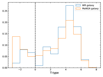
Figure 8: The morphology histogram of MaNGA and WR population. Both sample have been applied the volume correction. $T$-type value is an indicator of morphology type with negative values indicating early-type morphologies and positive values being late-type morphologies. Errorbars are Poisson counting error. All early-type WR galaxies are found to be S0 galaxies.

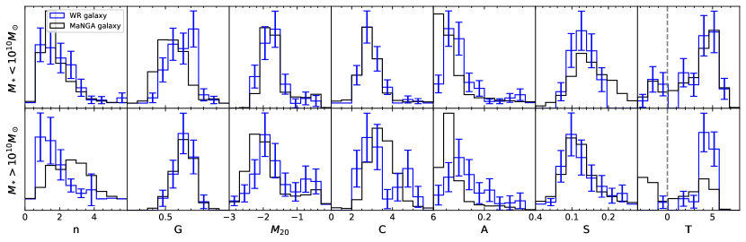
Figure 9: Distribution of structural parameters of WR galaxies (in blue) in comparison with general population reconstructed from MaNGA galaxies with weights (in black). Errorbars are Poisson counting error. The upper panels are for low-mass galaxies with $M_{*}<10^{10}M_{\odot}$ while the lower panels are for high-mass galaxies with $M_{*}>10^{10}M_{\odot}$. Panels from left to right are for different structural parameters: Sérsic index $n$, Gini index $G$, second-order moment of light $M_{20}$, concentration index $C$, rotational asymmetry A, and clumpiness S, as well as the morphological $T$-type. The vertical dashed lines in $T$-type panels indicate the empirical division between late-type (positive $T$) and early-type (negative $T$) galaxies. All early-type WR galaxies are also classified as S0 lenticular galaxies.

Figure 10: The $G$ versus $M_{20}$ diagram for the WR galaxies with low (upper) and high (lower) stellar masses. The grey-scale background is the distribution of general population of galaxies reconstructed from the MaNGA MPL-7 sample with weights. Blue dots are WR galaxies with S0-type WR galaxies highlighted with an additional red circle. Two diagnostic lines separating merging systems from normal galaxies are from Lotz et al. (2008, solid) and Lotz et al. (2004, dashed).

In Figure 9 we show the distribution of structural parameters, comapring the WR galaxy sample with the MaNGA sample. For both samples we have weighted each galaxy using the weights provided from the MaNGA MPL-7 release. The structural parameters are measured by Pawlik et al. (2016) by applying a range of automated structural measures to the sky-subtracted $r$-band SDSS images. These include $n$ (Sérsic index to measure the power-law index in fitting the radial surface brightness profile), $G$ (Gini index to measure the degree of inequality in the light ditribution), $M_{20}$ (second-order moment of the flux-weighted distance of the brightnest pixels containing 20% of the total light), $C$ (concentration index defined by five times the logarithmic ratio of the radii enclusing 80% and 20% of the total light), $A$ (rotational asymmetry), and $S$ (clumpiness). Definitions of these parameters are detailed in § 3.2 of Pawlik et al. (2016).

As can be seen, the general population of galaxies show clear dependence on mass in all the prameters, in the sense that galaxies of lower masses have lower values of $n$, $G$ and $C$, higher values of $M_{20}$ and $S$, and similar values of $A$. In contrast, the WR galaxy sample appears to show no or weak mass dependence, with the two mass subsamples showing very similar distributions in all parameters. As a result, the WR galaxies share the same distributions of $n$, $M_{20}$ and $C$ as the general population of low-mass galaxies, while they are the same as the high-mass general population in terms of $G$ and $S$. At both masses the WR galaxies are more asymmetric than the general population, indicating a higher-than-average fraction of interacting/merging systems in the WR galaxy sample. In the rightmost panels we show the distributions of the morphological $T$-type again, but for the two mass ranges separately. At low masses the WR sample shows the same $T$-type distribution as the general population. At high masses the WR galaxies are limited to late-type morphologies with few galaxies with $T<0$. Therefore, the WR galaxies of S0 type as previously seen in Figure 8 are mostly at low masses.

In Figure 10 we show the distribution of WR galaxies (blue dots) and general population for comparison (grey-scale background) on the plane of $G$ versus $M_{20}$. The general population is reconstructed from MaNGA MPL-7 sample with weights. The diagram is separate for the two mass intervals divided at $10^{10}M_{\odot}$. The higher $G$ of the WR sample at low masses and their lower $M_{20}$ at high masses, as seen in the previous figure, are also clearly seen here. As a result, the WR galaxies at both masses are preferentially found in the area of “merging systems”, as defined by the empirical diagnostic lines from Lotz et al. (2008) and Lotz et al. (2004) which are plotted as the solid and dashed lines in the figure. This result is consistent with the larger-than-average asymmetry of the WR sample as found in the previous figure.

To further understand the merging fraction of the WR sample, we have separated the WR galaxies in interacting systems from the non-interacting WR galaxies using the pair galaxy catalog from Fu et al. (2018), who identified interacting and merging galaxies in MaNGA MPL5 and later extended to MaNGA MPL6 (basically identical to MPL7) by the criteria of “projected separations less than 30 kpc, radial velocity offsets less than 600 km s^-1, and mass ratios greater than 0.1”. We find 43 out of the 90 WR galaxies (47.8%) to be interacting galaxies or mergers, a fraction that is much higher than that of the general population. This strongly suggests that the WR galaxies, as identified usually with strong star formation, are closely associated with galaxy-galaxy interactions. This finding is consistent with the known effect that tidal interactions between galaxies can effectively enhance the star formation in galactic centers (e.g. Li et al., 2008).

4 Discussion

4.1 Comparison with SDSS-based catalogs

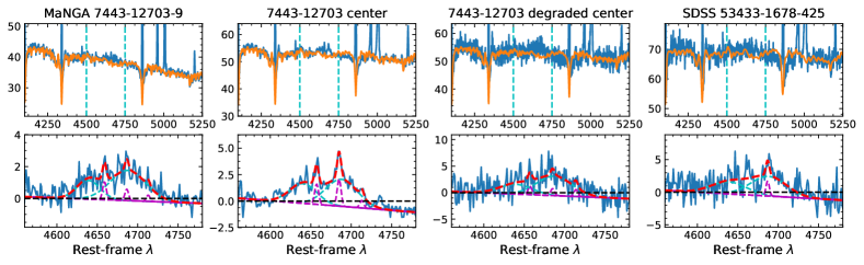
Figure 11: Comparison with SDSS spectra. Four sets of panels are shown. Each set is one example galaxy of the following categories: WR galaxies missed by SDSS studies purely due to low spectral S/N, WR galaxies missed by SDSS studies due to a difference in fitting models (also related to low spectral S/N), WR galaxies showing WR features even in SDSS spectra but missed by SDSS studies due to unclear reasons, and one WR galaxy identified by SDSS studies but missed by this work. In each set, the top row shows the observed spectra and the respective fitting models for them, and the bottom row shows the residual spectra in the zoom-in WR wavelength range with a tentative WR bump fitting. The first column in each set shows the central WR region; the second column is the stacked central 3″-diameter spectrum; the third column is the degraded second column to match the S/N of the fourth column, which is the original SDSS spectra.

Zhang et al. (2007) selected 174 WR galaxies from SDSS data release 3 (DR3), while Brinchmann et al. (2008) selected 570 WR galaxies from SDSS data release 6 (DR6). The fractions of WR galaxies are 0.05% and 0.08% without correcting for incompleteness due to flux limit or other selection effects. The SDSS observed only the central 1-2 kpc of the galaxies using a single fiber of 3″ diameter. Out of the 90 WR galaxies selected from the MaNGA MPL-7 in this work, we find 46 galaxies to have a central WR region, i.e. they have at least one WR region whose center spaxel is located within the central 3″-diameter region. Among these 46 galaxies, 39 are in SDSS DR6, whiles others are added from SDSS DR7 or the SDSS-III BOSS project. Of the 39 galaxies, only 7 are included in the catalog of Zhang et al. (2007) or Brinchmann et al. (2008). In other words, the SDSS-based catalogs have missed most of the WR galaxies from MaNGA (i.e. 32/39), even when we only consider the WR regions in galactic centers.

In order to understand why the SDSS-based studies failed to identify these 32 galaxies, we have done a one-to-one comparison between SDSS data and MaNGA data, and we find multiple reasons. Before we start the detailed comparison, for six galaxies, we find the SDSS fiber was positioned on an off-center region, and so the central WR region is outside the SDSS fiber but covered by the MaNGA IFU. These six galaxies should not be counted as missing WR galaxies in previous studies.

In the remaining 26 comparisons, first of all, about 70% of the missing galaxies (18/26) should be attributed to the low S/N of the SDSS spectra. In Figure 11, as an example, row No.1-2 show spectra and WR bumps of the central WR region from MaNGA (left-most panel) and the SDSS spectrum of the same galaxy (right-most panel). The upper panels show the observed spectrum and the best-fit stellar spectrum from 4000-5250 Å, and the lower panels show the starlight-subtracted spectrum over the WR bump wavelengths. We obtain the best-fit stellar spectrum for all the cases using our fitting code (see § 2.4). We note that the central WR region may cover different area than the SDSS fiber, and the spectra from the two surveys have different S/N. To have a more direct comparison, we have obtained the integrated spectrum over the central 3″-diameter region (i.e. the same as covered by the SDSS fiber) with our stacking code from the MaNGA datacube. The observed, best-fit and residual spectra are shown in the second column in which the WR feature is similarly seen. The third column shows the MaNGA spectra of the central 3″-diameter region again, but random noise is added to the observed spectrum so as to have the same S/N as the SDSS spectrum. As can be seen, like the SDSS spectrum, the WR bump becomes very weak and the region would be unlikely to be identified as a WR region.

For the remaining eight galaxies, we find five galaxies can also be attributed to their low spectral S/N, but in a different manner — they were missed due to uncertainties in the spectral fitting of low quality spectra. Row No. 3-4 of Figure 11 shows an example galaxy in this case. For this galaxy, the WR bump is still significant (though weaker) after the S/N of the spectrum is reduced to match the S/N of the SDSS spectrum. However, the residual spectrum of the SDSS shows almost no feature in the WR wavelength window. Looking closely at the upper panels in the third and the last column of the second row, we find the best-fit stellar spectra indeed differ slightly. This indicates that the identification of WR features could be affected by spectral fitting especially when the S/N of the spectrum is relatively low. Finally, for the last three galaxies, we find their WR feature remains after the S/N is reduced, and this is true also for the SDSS spectrum. Row No. 5-6 of the figure displays one of the three galaxies as an example. They were missed by previous studies possibly because of different criteria in visual inspection, their different fitting recipes or other serendipitous reasons.

We conclude that the much lower detection rate of WR galaxies in the SDSS is caused by multiple reasons. Among all reasons, the limited spatial coverage of the single-fiber spectroscopy and the relatively low spectral S/N are the main reasons, which can respectively explain about a half and 70% in the remaining half of WR galaxies that were missed in previous SDSS-based studies.

We should point out that, there is only one galaxy which was identified to be a WR galaxy in SDSS-based studies but is not included in our WR galaxy catalog. The observed, best-fit and residual spectra of this galaxy are shown in the bottom two rows of Figure 11. As can be seen, the galaxy presents a blue bump in all cases, indeed, although it appears to be more pronounced in the SDSS spectrum. This galaxy is missed in our case, likely due to the relatively strict criterion of our visual inspection. We tend not to add this galaxy to our catalog to keep the consistency of our selection procedure. We should keep in mind, however, that the detection fraction of WR galaxies in our study should be regarded as a lower limit, although it is much closer to the real fraction when compared to the SDSS catalogs.

4.2 Comparison with CALIFA-based catalog

Although the MaNGA sample gives a much higher detection rate than previous SDSS samples, the WR galaxy fraction ($1-2$% at most stellar masses, see Figure 5) is a bit too low when compared to the CALIFA sample which includes a fraction of $\sim$4.5% WR galaxies (Miralles-Caballero et al., 2016). This difference can be explored from a couple of factors. The first is the different spatial coverages of the CALIFA and MaNGA IFUs. Although CALIFA covers galaxies out to their 3-4 $R_{e}$, which is larger than the 1.5$R_{e}$ and 2.5$R_{e}$ covered by the MaNGA Primary and Secondary samples, we find that all WR regions in CALIFA galaxies are located within 1.5 $R_{e}$. Therefore, the spatial coverage of the IFUs should not cause any difference in the WR galaxy fraction. Secondly, we consider the possible effect of the different spatial resolutions. The angular resolutions are 2.5″ for both surveys (Law et al., 2016; García-Benito et al., 2015). Given the different redshifts and field of views of the two surveys, the physical resolution (in unit of kpc) and the relative resolution (in unit of $R_{e}$) could both be different. We discuss these two factors below.

The physical resolution is mainly determined by redshift given the same angular resolution. We find that most CALIFA WR galaxies (11 out of 15 from the main sample, 20 out of 25 from the entire sample) are below $z=0.01$ while MaNGA galaxy sample has a lower limit of $z=0.01$. The CALIFA parent sample has an approximately uniform distribution from $z=0$ to $z=0.03$. Therefore, it is apparent that when we limit the redshift range to $0.01<z<0.03$, CALIFA detection rate becomes pretty low. As for MaNGA, the volume-corrected detection rate in $0.01<z<0.03$ increase to 2.28%, due to a better physical resolution at lower redshift. In z=0.01-0.02, see Figure 12, MaNGA and CALIFA have very similar WR fraction. In z=0.02-0.03, CALIFA has no WR galaxy detected, maybe due to Poisson fluctuation with its relatively small sample size. The much higher detection rate from CALIFA at $z<0.01$ may imply the real WR galaxy rate is still higher than the fraction of CALIFA and MaNGA studies. Overall, due to small number statistics, we are not sure whether the high overall fraction of CALIFA WR is entirely due to the contribution from $z=0-0.01$.

Figure 12: WR fraction as a function of redshift for both MaNGA (blue dots) and CALIFA (orange stars) catalogs. Both fractions have been applied the volume correction.

Then we consider the relative resolution. With the CALIFA field of view and survey design, the angular diameter of its galaxies are typically 2-4 times larger than MaNGA galaxies. So with the same angular resolution, CALIFA sample have a better relative resolution with regard to $R_{e}$. Since the overlap of galaxy size between CALIFA and MaNGA is pretty small, we can hardly construct subsamples from the two surveys with the same distribution, and thus we resort to another approach for testing this factor. We use MaNGA sample to examine whether the detection rate has a trend with galaxy size. Size is correlated with other basic properties over the process of galaxy evolution, for example mass, which significantly affects WR rate as shown previously. Thus, we control mass when examining the correlation of WR rate with size, as mass is the most driving dependency of WR rate among basic properties of galaxies. Our result shows a slight decrease of detection rate towards larger galaxy size, on the contrary to the higher detection rate of CALIFA with its larger galaxy sizes. Since there is large uncertainty on the trend due to small number of statistics, we limit our discussion to this phenomenological trend and leave the validation of the trend as well as physical interpretation to future studies.

Next, we consider the difference in parameter distributions of galaxies in the two surveys which may also contribute to the different detection rates. Both CALIFA and MaNGA consist of a main sample and some ancillary programs. The ancillary programs mostly target peculiar galaxies and therefore increase the uncertainty and difficulty of constraining the WR fraction. For this reason, we limit our discussion here to WR galaxy fraction in main samples of the two surveys. For CALIFA we discard the extension sample, and for MaNGA, we keep the primary sample and secondary sample while excluding the color-enhanced sample and galaxies from ancillary programs. For the CALIFA sample, 15 out of the 25 WR galaxies are from its 448 main sample galaxies (Miralles-Caballero et al., 2016). In the case of MaNGA, 60 out of the 90 WR galaxies are from its 3735 unique Primary or Secondary sample galaxies. Without any corrections, the WR galaxy fraction is 3.35% and 1.61% for CALIFA and MaNGA, respectively. Considering the mass dependence of the WR galalaxy detection as shown in Figure 4, we construct a control sample of galaxies from the MaNGA Primary and Secondary samples that have the same distribution in stellar mass as the CALIFA main sample. We find a WR galaxy fraction of $1.26\pm 0.14$% in this control sample. Furthermore, we require the control sample of MaNGA galaxies to have the same distribution as CALIFA in both stellar mass and $NUV-r$ color, to take into account potential effect of different colors of the two samples. To this end, we have trimmed both samples so that they have similar distributions of galaxies in the two-dimensional mass—color space. The resulting WR galaxy fractions are $1.63\pm 0.24\%$ for MaNGA and $3.68\pm 0.95\%$ for CALIFA. The errors are Poisson counting error. Therefore, we conclude that the different WR galaxy detection rates between the two surveys are not caused by the different properties of the galaxies.

Also, MaNGA and CALIFA spectra have similar S/N distribution. Therefore, S/N should not be a significant reason for the difference in WR fraction.

Finally, we notice that the WR galaxy catalogs from both CALIFA and MaNGA have a large fraction of merging systems. We use Walcher et al. (2014) for classification of CALIFA galaxies and the extended version of Fu et al. (2018) for classification of MaNGA galaxies. By separating mergers and isolated galaxies, we find the WR fraction in isolated galaxies is $3.15\pm 0.8\%$ for CALIFA and $1.41\pm 0.20$% for MaNGA. Errors are Poisson counting errors. The difference is still significant. Therefore, we claim the difference in WR fractions of the two surveys is unlikely to be caused by the merger fraction in their parent samples. But we also want to point out that due to the small numbers in statistics and the subjectivity in classification of mergers, we still need better data and classification to explore the effect of mergers on WR fraction in the future.

To conclude, the higher WR galaxy fraction in the CALIFA sample may be explained mainly by the inclusion of galaxies at $z<0.01$. Above the MaNGA redshift limit $z=0.01$, the WR galaxy fractions from the two surveys are actually very similar. Other factors, whether physical or instrumental, do not have a clear or significant contribution in the difference between this work and CALIFA WR catalog.

4.3 Abundance of WR galaxies

Throughout the construction of this catalog, we put much emphasis on purity, especially in the careful choice of full spectrum fitting recipe and visual inspection. As for the completeness, we suspect that there should always be some weak WR population that is beneath the detection capability of our data quality. For example, in the determination of H II regions, we adopt a high threshold for $H\alpha$ surface brightness, which may possibly miss some WR regions. Therefore, our WR fraction of $1.9\pm 0.2\%$ should be considered as lower limits of the real fractions. The higher WR detection rate of CALIFA, as discussed above, also indicates that the WR galaxy fraction could be even higher if IFU surveys with higher resolution and S/N are available.

4.4 Coexistence of WR features and Active Galactic Nuclei

There are three WR galaxies in our catalog that show either AGN-like broad emission lines or Seyfert line ratios on the BPT diagram (Baldwin et al., 1981; Kewley et al., 2001; Kauffmann et al., 2003; Kewley et al., 2006). For example, the outlier at redshift z$\simeq$0.11 in Figure 3 is one of them. We carefully examined the spectra, spatially-resolved BPT diagram, Fe emission line template from (Véron-Cetty et al., 2004), etc. We conclude all these galaxies show real WR features with possible simultaneous existence of AGN. For example, galaxy 8626-12704 has a clear WR red bump. We also find a few WR regions classified as ”composite of star-forming and AGN activities” on the BPT diagram and these galaxies may carry specific scientific interest. With the coexistence of WR population and AGN, it is possible to study the interaction between AGN and recent star-formation in the future.

4.5 Red bump

As mentioned earlier, besides the blue bump, WR stars also form a red bump around 5800 Å with C and N broad emission lines. Normally the red bump feature is weaker than the blue bump. With our WR catalog, we visually examine the wavelength range of the red bump and find 39 WR regions from 24 WR galaxies show red bumps. The weakness of the red bump is not only reflected in the small number of occurrence but also in the significance of individual occurrences, and therefore these identifications carry higher uncertainty compared to the blue bump identifications. With these red bumps, together with information from the blue bumps, we can further derive the ratio among different WR subtypes. We will leave this part to the parallel paper discussing spatially resolved properties of WR regions.

5 Conclusions

In this work we have carried out a thorough search for WR galaxies from MaNGA MPL7 (i.e. SDSS DR15) data. We develop a two-step searching scheme to tackle the challenge of the weakness of WR features. We start by identifying H II regions in the MaNGA datacubes. We obtain a high S/N spectrum for each region by stacking the original spectra, and perform full spectral fitting to the stacked spectrum. Next, we visually examine the starlight-subtracted spectrum of all the H II regions, and identify WR regions according to the presence of a blue bump at $4600-4750$ Å as signature of the WR stars. The resulting WR catalog consists of 267 WR regions, distributed in 90 WR galaxies, which is 1.9% of the parent sample. This fraction is much higher than previous stuidies based on single fiber SDSS data, and similar to the recent study based on CALIFA IFU data. Through detailed comparisons with SDSS and CALIFA surveys, we evaluate the impact of different survey parameters on WR fraction, and show consistency between this work and previous studies. We have examined the global properties of the WR galaxies, and for the first time estimated the stellar mass function of WR galaxies.

Our main conclusions can be summarized as follows.

• WR regions are exclusively found in galaxies that show bluest colors and highest star formation rates for their mass, as well as late-type dominated morphologies. Their images have relatively high asymmetry, indicative of a higher-than-average fraction of mergers in the WR population.

• The stellar mass function of WR galaxies can well be described by a Schechter function with amplitude $\phi_{*}$ = 0.000157 Mpc^-3, characteristic mass $log_{10}(M^{*}/M_{\odot})$ = 10.332, and the faint-end slope $\alpha$ = -0.905. This gives rise to an average number density of $3.47\times 10^{-4}Mpc^{-3}$ and an average detection rate of 1.4% with respect to the general population of galaxies in the Local Universe. The detection rate shows weak dependence on stellar mass, with a maximum of $\sim 4$% at $M_{\ast}\sim 10^{9.7}M_{\odot}$.

• The small fraction of WR galaxies found previously in SDSS-based samples is attributed mainly to two facts. One is the single-fiber spectroscopy covering a limited central region of galaxies. The second fact is the lower S/N of the SDSS spectra compared to MaNGA. About half of our WR galaxies show WR features in their centers, but most of them were missed by previous SDSS studies due to the low S/N of the SDSS spectra.

• The CALIFA finds a higher fraction of WR galaxies than MaNGA mainly due to the inclusion of galaxies at $z<0.01$, which have better spatial resolution (in unit of pc) than galaxies at higher redshift.

There are still some limitations of this study for future improvements. Although MaNGA has its unique advantage of a large sample size, allowing us to construct a large catalog of new WR galaxies, its S/N and spatial resolution are not ideal for WR search. Random error of spectra may cause false positive identification in a few cases while the current spatial resolution may lead to loss of some compact WR regions due to dilution effect. Furthermore, the weak WR feature is very sensitive to full spectrum fitting recipe. The flux calibration of fitting templates, the masking of emission lines, the fitting code and fitting procedure in use, etc. may all affect the WR feature in the fitting residual. In the future, better templates such as SSPs derived from MaStar stellar library (Nair & Abraham, 2010) and deeper exposure will probably improve this study. Nevertheless, our catalog includes a large number of WR regions from galaxies covering wide ranges in mass and color, and so it should be able to form a good basis for many future studies. In fact, the current paper is the first of a series of works in which we will perform extensive studies of the WR regions/galaxies. The next paper will include resolved mass-metallicity relation of WR regions. Also, WR subtype ratios will be studied as a function of metallicity and stellar population age. Moreover, both WR blue bumps and red bumps will be compared to model predictions from Starburst99 (Schaerer & Vacca, 1998) and BPASS (Eldridge et al., 2017) to constrain the metallicity-dependent variation of the stellar initial mass function.

References

- Agienko et al. (2013) Agienko, K. B., Guseva, N. G., & Izotov, Y. I. 2013, Kinematics and Physics of Celestial Bodies, 29, 131, doi: 10.3103/S0884591313030021
- Aguado et al. (2019) Aguado, D. S., Ahumada, R., Almeida, A., et al. 2019, ApJS, 240, 23, doi: 10.3847/1538-4365/aaf651
- Allen et al. (1976) Allen, D. A., Wright, A. E., & Goss, W. M. 1976, MNRAS, 177, 91, doi: 10.1093/mnras/177.1.91
- Anderson et al. (2019) Anderson, L. D., Wenger, T. V., Armentrout, W. P., Balser, D. S., & Bania, T. M. 2019, ApJ, 871, 145, doi: 10.3847/1538-4357/aaf571
- Baldwin et al. (1981) Baldwin, J. A., Phillips, M. M., & Terlevich, R. 1981, PASP, 93, 5, doi: 10.1086/130766
- Bergvall & Östlin (2002) Bergvall, N., & Östlin, G. 2002, A&A, 390, 891, doi: 10.1051/0004-6361:20020759
- Blanton et al. (2011) Blanton, M. R., Kazin, E., Muna, D., Weaver, B. A., & Price-Whelan, A. 2011, AJ, 142, 31, doi: 10.1088/0004-6256/142/1/31
- Blanton et al. (2017) Blanton, M. R., Bershady, M. A., Abolfathi, B., et al. 2017, AJ, 154, 28, doi: 10.3847/1538-3881/aa7567
- Brinchmann et al. (2004) Brinchmann, J., Charlot, S., White, S. D. M., et al. 2004, MNRAS, 351, 1151, doi: 10.1111/j.1365-2966.2004.07881.x
- Brinchmann et al. (2008) Brinchmann, J., Kunth, D., & Durret, F. 2008, A&A, 485, 657, doi: 10.1051/0004-6361:200809783
- Bundy et al. (2015) Bundy, K., Bershady, M. A., Law, D. R., et al. 2015, ApJ, 798, 7, doi: 10.1088/0004-637X/798/1/7
- Chabrier (2003) Chabrier, G. 2003, PASP, 115, 763, doi: 10.1086/376392
- Cherinka et al. (2019) Cherinka, B., Andrews, B. H., Sánchez-Gallego, J., et al. 2019, AJ, 158, 74, doi: 10.3847/1538-3881/ab2634
- Crowther (2007) Crowther, P. A. 2007, ARA&A, 45, 177, doi: 10.1146/annurev.astro.45.051806.110615
- Domínguez Sánchez et al. (2018) Domínguez Sánchez, H., Huertas-Company, M., Bernardi, M., Tuccillo, D., & Fischer, J. L. 2018, MNRAS, 476, 3661, doi: 10.1093/mnras/sty338
- Drissen et al. (1993) Drissen, L., Roy, J.-R., & Moffat, A. F. J. 1993, AJ, 106, 1460, doi: 10.1086/116739
- Drory et al. (2015) Drory, N., MacDonald, N., Bershady, M. A., et al. 2015, AJ, 149, 77, doi: 10.1088/0004-6256/149/2/77
- Eldridge et al. (2017) Eldridge, J. J., Stanway, E. R., Xiao, L., et al. 2017, PASA, 34, e058, doi: 10.1017/pasa.2017.51
- Falcón-Barroso et al. (2011) Falcón-Barroso, J., Sánchez-Blázquez, P., Vazdekis, A., et al. 2011, A&A, 532, A95, doi: 10.1051/0004-6361/201116842
- Fu et al. (2018) Fu, H., Steffen, J. L., Gross, A. C., et al. 2018, ApJ, 856, 93, doi: 10.3847/1538-4357/aab364
- Garay & Lizano (1999) Garay, G., & Lizano, S. 1999, PASP, 111, 1049, doi: 10.1086/316416
- García-Benito et al. (2015) García-Benito, R., Zibetti, S., Sánchez, S. F., et al. 2015, A&A, 576, A135, doi: 10.1051/0004-6361/201425080
- Gunn et al. (2006) Gunn, J. E., Siegmund, W. A., Mannery, E. J., et al. 2006, AJ, 131, 2332, doi: 10.1086/500975
- Guseva et al. (2000) Guseva, N. G., Izotov, Y. I., & Thuan, T. X. 2000, ApJ, 531, 776, doi: 10.1086/308489
- Hsieh et al. (2017) Hsieh, B. C., Lin, L., Lin, J. H., et al. 2017, ApJ, 851, L24, doi: 10.3847/2041-8213/aa9d80
- Hunt & Hirashita (2009) Hunt, L. K., & Hirashita, H. 2009, A&A, 507, 1327, doi: 10.1051/0004-6361/200912020
- Husemann et al. (2013) Husemann, B., Jahnke, K., Sánchez, S. F., et al. 2013, A&A, 549, A87, doi: 10.1051/0004-6361/201220582
- Kauffmann et al. (2003) Kauffmann, G., Heckman, T. M., Tremonti, C., et al. 2003, MNRAS, 346, 1055, doi: 10.1111/j.1365-2966.2003.07154.x
- Kennicutt (1984) Kennicutt, R. C., J. 1984, ApJ, 287, 116, doi: 10.1086/162669
- Kewley et al. (2001) Kewley, L. J., Dopita, M. A., Sutherland, R. S., Heisler, C. A., & Trevena, J. 2001, ApJ, 556, 121, doi: 10.1086/321545
- Kewley et al. (2006) Kewley, L. J., Groves, B., Kauffmann, G., & Heckman, T. 2006, MNRAS, 372, 961, doi: 10.1111/j.1365-2966.2006.10859.x
- Kim & Koo (2001) Kim, K.-T., & Koo, B.-C. 2001, ApJ, 549, 979, doi: 10.1086/319447
- Kunth & Joubert (1985) Kunth, D., & Joubert, M. 1985, A&A, 142, 411
- Law et al. (2016) Law, D. R., Cherinka, B., Yan, R., et al. 2016, AJ, 152, 83, doi: 10.3847/0004-6256/152/4/83
- Le Borgne et al. (2003) Le Borgne, J. F., Bruzual, G., Pelló, R., et al. 2003, A&A, 402, 433, doi: 10.1051/0004-6361:20030243
- Li et al. (2008) Li, C., Kauffmann, G., Heckman, T. M., Jing, Y. P., & White, S. D. M. 2008, MNRAS, 385, 1903, doi: 10.1111/j.1365-2966.2008.13000.x
- Li et al. (2005) Li, C., Wang, T.-G., Zhou, H.-Y., Dong, X.-B., & Cheng, F.-Z. 2005, AJ, 129, 669, doi: 10.1086/426909
- Li & White (2009) Li, C., & White, S. D. M. 2009, MNRAS, 398, 2177, doi: 10.1111/j.1365-2966.2009.15268.x
- Lopez et al. (2011) Lopez, L. A., Krumholz, M. R., Bolatto, A. D., Prochaska, J. X., & Ramirez-Ruiz, E. 2011, ApJ, 731, 91, doi: 10.1088/0004-637X/731/2/91
- Lotz et al. (2004) Lotz, J. M., Primack, J., & Madau, P. 2004, AJ, 128, 163, doi: 10.1086/421849
- Lotz et al. (2008) Lotz, J. M., Davis, M., Faber, S. M., et al. 2008, ApJ, 672, 177, doi: 10.1086/523659
- Miralles-Caballero et al. (2014) Miralles-Caballero, D., Rosales-Ortega, F. F., Díaz, A. I., et al. 2014, MNRAS, 445, 3803, doi: 10.1093/mnras/stu2002
- Miralles-Caballero et al. (2016) Miralles-Caballero, D., Díaz, A. I., López-Sánchez, Á. R., et al. 2016, A&A, 592, A105, doi: 10.1051/0004-6361/201527179
- Nair & Abraham (2010) Nair, P. B., & Abraham, R. G. 2010, ApJS, 186, 427, doi: 10.1088/0067-0049/186/2/427
- Osterbrock & Cohen (1982) Osterbrock, D. E., & Cohen, R. D. 1982, ApJ, 261, 64, doi: 10.1086/160318
- Pawlik et al. (2016) Pawlik, M. M., Wild, V., Walcher, C. J., et al. 2016, MNRAS, 456, 3032, doi: 10.1093/mnras/stv2878
- Pérez-Montero et al. (2013) Pérez-Montero, E., Kehrig, C., Brinchmann, J., et al. 2013, Advances in Astronomy, 2013, 837392, doi: 10.1155/2013/837392
- Sánchez et al. (2012a) Sánchez, S. F., Rosales-Ortega, F. F., Marino, R. A., et al. 2012a, A&A, 546, A2, doi: 10.1051/0004-6361/201219578
- Sánchez et al. (2012b) Sánchez, S. F., Kennicutt, R. C., Gil de Paz, A., et al. 2012b, A&A, 538, A8, doi: 10.1051/0004-6361/201117353
- Schaerer et al. (1999) Schaerer, D., Contini, T., & Pindao, M. 1999, A&AS, 136, 35, doi: 10.1051/aas:1999197
- Schaerer & Vacca (1998) Schaerer, D., & Vacca, W. D. 1998, ApJ, 497, 618, doi: 10.1086/305487
- Schechter (1976) Schechter, P. 1976, ApJ, 203, 297, doi: 10.1086/154079
- Sérsic (1963) Sérsic, J. L. 1963, Boletin de la Asociacion Argentina de Astronomia La Plata Argentina, 6, 41
- Shirazi & Brinchmann (2012) Shirazi, M., & Brinchmann, J. 2012, MNRAS, 421, 1043, doi: 10.1111/j.1365-2966.2012.20439.x
- Smee et al. (2013) Smee, S. A., Gunn, J. E., Uomoto, A., et al. 2013, AJ, 146, 32, doi: 10.1088/0004-6256/146/2/32
- van der Hucht (2001) van der Hucht, K. A. 2001, New A Rev., 45, 135, doi: 10.1016/S1387-6473(00)00112-3
- Vazdekis et al. (2010) Vazdekis, A., Sánchez-Blázquez, P., Falcón-Barroso, J., et al. 2010, MNRAS, 404, 1639, doi: 10.1111/j.1365-2966.2010.16407.x
- Vazdekis et al. (2015) Vazdekis, A., Coelho, P., Cassisi, S., et al. 2015, MNRAS, 449, 1177, doi: 10.1093/mnras/stv151
- Véron-Cetty et al. (2004) Véron-Cetty, M. P., Joly, M., & Véron, P. 2004, A&A, 417, 515, doi: 10.1051/0004-6361:20035714
- Wake et al. (2017) Wake, D. A., Bundy, K., Diamond-Stanic, A. M., et al. 2017, AJ, 154, 86, doi: 10.3847/1538-3881/aa7ecc
- Walcher et al. (2014) Walcher, C. J., Wisotzki, L., Bekeraité, S., et al. 2014, A&A, 569, A1, doi: 10.1051/0004-6361/201424198
- Westfall et al. (2019) Westfall, K. B., Cappellari, M., Bershady, M. A., et al. 2019, arXiv e-prints, arXiv:1901.00856
- Willett et al. (2013) Willett, K. W., Lintott, C. J., Bamford, S. P., et al. 2013, MNRAS, 435, 2835, doi: 10.1093/mnras/stt1458
- Wolf & Rayet (1867) Wolf, C. J. E., & Rayet, G. 1867, Academie des Sciences Paris Comptes Rendus, 65, 292
- Yan et al. (2016a) Yan, R., Tremonti, C., Bershady, M. A., et al. 2016a, AJ, 151, 8, doi: 10.3847/0004-6256/151/1/8
- Yan et al. (2016b) Yan, R., Bundy, K., Law, D. R., et al. 2016b, AJ, 152, 197, doi: 10.3847/0004-6256/152/6/197
- York et al. (2000) York, D. G., Adelman, J., Anderson, John E., J., et al. 2000, AJ, 120, 1579, doi: 10.1086/301513
- Zhang et al. (2017) Zhang, K., Yan, R., Bundy, K., et al. 2017, MNRAS, 466, 3217, doi: 10.1093/mnras/stw3308
- Zhang et al. (2007) Zhang, W., Kong, X., Li, C., Zhou, H.-Y., & Cheng, F.-Z. 2007, ApJ, 655, 851, doi: 10.1086/510231