Stieltjes moment sequences
for pattern-avoiding permutations

Abstract

A small set of combinatorial sequences have coefficients that can be represented as moments of a nonnegative measure on $[0,\infty)$. Such sequences are known as Stieltjes moment sequences. They have a number of nice properties, such as log-convexity, which are useful to rigorously bound their growth constant from below.

This article focuses on some classical sequences in enumerative combinatorics, denoted $Av(\mathcal{P})$, and counting permutations of $\{1,2,\ldots,n\}$ that avoid some given pattern $\mathcal{P}$. For increasing patterns $\mathcal{P}=(12\ldots k)$, we recall that the corresponding sequences, $Av(123\ldots k)$, are Stieltjes moment sequences, and we explicitly find the underlying density function, either exactly or numerically, by using the Stieltjes inversion formula as a fundamental tool.

We first illustrate our approach on two basic examples, $Av(123)$ and $Av(1342)$, whose generating functions are algebraic. We next investigate the general (transcendental) case of $Av(123\ldots k)$, which counts permutations whose longest increasing subsequences have length at most $k-1$. We show that the generating functions of the sequences $\,Av(1234)$ and $\,Av(12345)$ correspond, up to simple rational functions, to an order-one linear differential operator acting on a classical modular form given as a pullback of a Gaussian $\,{}_{2}F_{1}$ hypergeometric function, respectively to an order-two linear differential operator acting on the square of a classical modular form given as a pullback of a $\,{}_{2}F_{1}$ hypergeometric function.

We demonstrate that the density function for the Stieltjes moment sequence $Av(123\ldots k)$ is closely, but non-trivially, related to the density attached to the distance traveled by a walk in the plane with $k-1$ unit steps in random directions.

Finally, we study the challenging case of the $Av(1324)$ sequence and give compelling numerical evidence that this too is a Stieltjes moment sequence. Accepting this, we show how rigorous lower bounds on the growth constant of this sequence can be constructed, which are stronger than existing bounds. A further unproven assumption leads to even better bounds, which can be extrapolated to give an estimate of the (unknown) growth constant.

Keywords: probability measure, density, moment problem, Stieltjes inversion formula, Stieltjes moment sequences, walks, Hankel determinants, piecewise functions, D-finite functions, pulled-back hypergeometric functions, classical modular forms.

1 Introduction

1.1 Context and motivation

Many important distributions in probability theory have moments that happen to coincide with some classical counting sequences in combinatorics. For instance, the moments of the standard exponential distribution $\mathcal{E}(1)$ with rate parameter 1,

$$a_{n}:=\int_{0}^{\infty}x^{n}\,\mu(x)\,dx,\qquad\hbox{with}\quad\mu(x):=e^{-x},$$ (1)

are equal to $a_{n}=n!$, and thus count the number of permutations of $\mathfrak{S}_{n}=\{1,\ldots,n\}$. Similarly, the moments of the standard Gaussian (normal) distribution $\mathcal{N}(0,1)$,

$$a_{n}:=\int_{0}^{\infty}x^{n}\,\mu(x)\,dx,\qquad\hbox{with}\quad\mu(x):=\frac{1}{\sqrt{2\pi}}e^{-x^{2}/2}$$ (2)

satisfy, for all $n\geqslant 0$,

$$a_{2n}=1\cdot 3\cdot 5\cdots(2n-1),\qquad a_{2n+1}=0,$$ (3)

so that $a_{2n}$ counts the number of pairings of $2n$ elements, or, equivalently, the number of perfect matchings of the complete graph $K_{2n}$.

Such connections between probability and combinatorics turn out to be useful in a number of contexts. For instance, Billingsley’s proof of the Central Limit Theorem by the “method of moments” [17, p. 408–410] arrives at a limiting Gaussian distribution (2), for sums of independent random variables, precisely thanks to the property of the corresponding moments to enumerate pairings (3).

In random graph theory, the Poisson distribution plays an important role. When the mean is $1$, its moments

$$a_{n}:={\mathbb{E}}(X^{n}),\qquad\hbox{where}\quad\mathbb{P}(X=k)=\frac{e^{-1}}{k!},$$ (4)

count the number of set partitions of a collection of $n$ elements, giving rise to the sequence of Bell numbers [50, p. 109–110]:

$$a_{n}=n!\times\left(\text{coefficient of }\;x^{n}\,\text{in}\;e^{e^{x}-1}\right).$$ (5)

It could be argued that the Poisson distribution arises, in many cases, from the emergence of set partitions, in accordance with Equations (4) and (5).

Random matrix theory also abounds with examples, the most famous case being Wigner’s semi–circle law. Here the Catalan numbers, $(C_{n})_{n\geqslant 0}=(1,1,2,5,14,42,\ldots)$, known to enumerate a variety of trees and lattice paths and given by the formula

$$C_{n}=\frac{1}{n+1}\binom{2n}{n}$$ (6)

appear, in the asymptotic limit, as (renormalized) expectations of powers of traces of random matrices in various ensembles. Their moment representation

$$C_{n+1}=\frac{1}{2\pi}\int_{0}^{4}x^{n}\,\sqrt{x(4-x)}\,dx$$

then implies convergence of the spectrum of the random matrices under consideration to the semicircle law with density $\frac{1}{2\pi}\sqrt{x(4-x)}$.

1.2 The main problem

There are thus good reasons to develop methods aimed at explicitly solving the so-called moment problem [112, 3], which considers a sequence ${\bf a}=(a_{n})_{n\geqslant 0}$ of real nonnegative numbers, and searches to express its general term $a_{n}$ as the integral

$$a_{n}=\int_{\Gamma}x^{n}d\rho(x)\qquad\text{for all}\;\;n\geqslant 0,$$

for some support $\Gamma\subseteq\mathbb{R},$ and for some probability measure $\rho$. In most cases one can write $d\rho(x)=\,\mu(x)\,dx,$ where $\mu(x)$ is a nonnegative function known as the probability density function of $\rho$ (in short, density), in which case the above equation becomes

$$a_{n}=\,\int_{\Gamma}x^{n}\,\mu(x)\,dx.$$ (7)

When in addition the support $\Gamma$ is a subset of the half-line $[0,\infty)$, the problem (7) is classically called the Stieltjes moment problem, and the sequence ${\bf a}\equiv(a_{n})_{n}$ a Stieltjes moment sequence. The same problem is called the Hausdorff moment problem when $\Gamma=[0,1]$ and the Hamburger moment problem when $\Gamma=\mathbb{R}$, see [69].

In this article, we will not consider the Hamburger moment problem, but only the Stieltjes and the Hausdorff problems. Note that a probability measure is entirely determined by its moments (i) in the Stieltjes case if $|a_{n}|\leqslant n!$ for all $n$ [17, Thm. 30.1], (ii) in the Hausdorff case, and more generally in the Stieltjes case with compact support [13], so that the problem (7) has a unique solution in those cases.

There are several necessary and sufficient conditions that the sequence ${\bf a}$ must satisfy in order to be a Stieltjes moment sequence, or equivalently, for a density function $\mu(x)$ to solve (7) for some support $\Gamma\subseteq[0,\infty]$. To express these conditions, one classically attaches to the sequence ${\bf a}$ the (infinite) Hankel matrices

$$H_{n}^{\infty}({\bf a})=\begin{bmatrix}a_{n}&a_{n+1}&a_{n+2}&\ldots\\ a_{n+1}&a_{n+2}&a_{n+3}&\ldots\\ a_{n+2}&a_{n+3}&a_{n+4}&\ldots\\ \vdots&\vdots&\vdots&\ddots\\ \end{bmatrix}.$$

The following classical result (see also [51, Thm. 2.8] and [116, Thm 2.2]), characterizes the property of being a Stieltjes moment sequence by using the Hankel matrices $H_{n}^{\infty}$. It was proved partly in 1894 by Stieltjes [120] and partly in 1937 by Gantmakher and Krein [53]. In particular, properties (a) and (d) were shown to be equivalent in [120], while these were later shown to be equivalent to (b) and (c) in [53, Th. 9], see also: (i) for (a)$\Longleftrightarrow$(b), [112, Thm. 1.3], [111, Thm. 3.12, p. 65], [131, Thm. 87.1, p. 327], [111, Thm. 3.12, p. 65], and [114, Thm. 1, p. 86]; (ii) for (b)$\Longleftrightarrow$(c), [53, Thm. 9], and [102, Thm. 4.4]; (iii) for (a)$\Longleftrightarrow$(d), [3, Appendix, Theorem 0.4, p. 237], and [99, Satz 4.14, p. 230; Satz 3.11, p. 120].

Theorem 1.

For a sequence ${\bf a}\equiv(a_{n})_{n\geqslant 0}$, the following are equivalent:

• There exist $\Gamma\subseteq[0,\infty)$ and a nonnegative measure $\rho$ on $\Gamma$ such that

  $$a_{n}=\,\int_{\Gamma}\,x^{n}\,d\rho(x).$$

• The matrices $H_{0}^{\infty}({\bf a})$ and $H_{1}^{\infty}({\bf a})$ are both positive semidefinite (i.e., all their leading principal minors, called Hankel determinants, are nonnegative).
  

• The matrix $H_{0}^{\infty}({\bf a})$ is totally nonnegative (i.e., all of its minors are nonnegative).
  

• There exists a sequence of nonnegative real numbers $(\alpha_{n})_{n\geqslant 0}$, such that the generating function $A(x)\,=\,\sum_{n=0}^{\infty}a_{n}x^{n}$ of the sequence ${\bf a}$ satisfies

  $$A(x)\,=\,\,\cfrac{\alpha_{0}}{1\,-\cfrac{\alpha_{1}x}{1-\,\cfrac{\alpha_{2}x}{\begin{array}[]{@{}c@{}c@{}c@{}}1\,-\cdots\end{array}}}}.$$

Moreover, the leading principal $n\times n$ minors $\Delta_{0}^{n}({\bf a})$ of $H_{0}^{\infty}({\bf a})$ and $\Delta_{1}^{n}({\bf a})$ of $H_{1}^{\infty}({\bf a})$ occurring in (b) are related to the coefficients $\alpha_{i}$ in the continued fraction (d) by:

$$\Delta_{0}^{n}({\bf a})=\alpha_{0}\cdot(\alpha_{1}\alpha_{2})^{n-1}\cdot(\alpha_{3}\alpha_{4})^{n-2}\cdots(\alpha_{2n-3}\alpha_{2n-2}),$$

$$\Delta_{1}^{n}({\bf a})=\alpha_{0}\cdot\alpha_{1}^{n}\cdot(\alpha_{2}\alpha_{3})^{n-1}\cdot(\alpha_{4}\alpha_{5})^{n-2}\cdots(\alpha_{2n-2}\alpha_{2n-1}).$$

One calls ${\bf a}$ a Stieltjes moment sequence if it satisfies the conditions of Theorem 1.

1.3 Examples

Geometric sequences $(\tau^{n})_{n\geqslant 0}$ with growth rate $\tau>0$ are Stieltjes moment sequences, as $\tau^{n}$ is equal to the $n$-th moment of the distribution with support $\Gamma={\{\tau\}}$ which is $\tau$ with probability 1; equivalently, one can take $\alpha_{0}=1,\alpha_{1}=\tau$ and $\alpha_{k}=0$ for $k\geqslant 2$ in (d). However, other very simple sequences with rational generating function are not Stieltjes; for instance, the Fibonacci sequence ${\bf a}=(1,1,2,3,5,8,\ldots)$ with generating function $1/(1-x-x^{2})$, is such that the second leading principal minor $\Delta_{1}^{2}({\bf a})$ of $H_{1}^{\infty}({\bf a})$ equals $1\times 3-2\times 2=-1<0$, and thus by (b) it cannot be Stieltjes. It is trivially a moment sequence for a linear combination of Dirac measures, hence it is a Hamburger moment sequence (with support $\Gamma$ included in $\mathbb{R}$ but not in $[0,\infty)$). More generally, Stieltjes moment sequences with rational generating functions are well-understood: for instance, if $(a_{n})_{n\geqslant 0}$ has a rational generating function with simple poles only, then $a_{n}$ is a finite sum of the form $\sum_{j}c_{j}p_{j}^{n}$ for some complex $c_{j},p_{j}$, the corresponding measure $\rho(x)$ is a weighted sum of Dirac measures $\sum_{j}c_{j}\delta(x-p_{j})$, and one has that $(a_{n})_{n\geqslant 0}$ is Stieltjes if and only if all $c_{j}$ and $p_{j}$ are nonnegative real numbers.

A useful refinement of Theorem 1 (see e.g., the references cited before its statement), which essentially excludes Stieltjes moment sequences whose generating functions are rational, is that: $(a^{\prime})$ ${\bf a}\equiv(a_{n})_{n\geqslant 0}$ is a Stieltjes moment sequence with a representing measure $\rho$ having infinite support $\Gamma$ (containing a dense subset of $\mathbb{R}$) $\Longleftrightarrow$ $(b^{\prime})$ $H_{0}^{\infty}({\bf a})$ and $H_{1}^{\infty}({\bf a})$ are both positive definite (i.e., all their leading principal minors are positive) $\Longleftrightarrow$ $(c^{\prime})$ $H_{0}^{\infty}({\bf a})$ is totally positive (i.e., all of its minors are positive) $\Longleftrightarrow$ $(d^{\prime})$ all the $\alpha_{i}$’s are positive.

Perhaps the simplest example of a Stieltjes moment sequence with irrational generating function is $a_{n}=\tau^{n+1}/(n+1)$ with $\tau>0$, which corresponds to the uniform distribution $\mathcal{U}(0,\tau)$, with $\Gamma=[0,\tau]$ and $\mu(x)\equiv 1$. Observe that the generating function $\sum_{n=0}^{\infty}a_{n}x^{n}=-{{\ln\left(1-\tau\,x\right)}/{x}}$ is not only irrational but already transcendental (i.e., non-algebraic). However, it is D-finite, i.e., it satisfies a linear differential equation with polynomial coefficients. Another basic example of Stieltjes sequence is $n!$, corresponding to the standard exponential distribution $\mathcal{E}(1)$ for which, according to (1), one can take $\Gamma=[0,\infty)$ and $\mu(x)=\exp(-x)$. This can also be seen by using $(d)$ and Euler’s 1746 continued fraction expansion [47, §21], with $\alpha_{0}=1$ and $\alpha_{2k-1}=\alpha_{2k}=k$ for $k\geqslant 1$. Once again, the generating function $\sum_{n\geqslant 0}n!x^{n}$ is D-finite, but not algebraic. More generally, Euler [47, §26] showed that for the sequence with general term $c\,(c+1)\cdots(c+n-1)$ one can take $\alpha_{2n-1}=c+n-1$ and $\alpha_{2n}=n$, so that the sequence is again Stieltjes for any real $c>0$, and its generating function is transcendental D-finite and satisfies the linear differential equation $L(y(x))=0$, where $L=$ ${x}^{2}D_{x}^{2}+\left((c+2)\,x-1\right)D_{x}+c=\left({x}^{2}D_{x}+2\,x\right)\left(D_{x}+{\frac{c\,x-1}{{x}^{2}}}\right)$. Here, and in all that follows, $D_{x}$ denotes the usual derivation operator $\frac{\partial}{\partial x}$.

A slightly more involved example is ${4^{n}\,(n+1)!\,n!}/{(2n+3)!}$ which is Stieltjes using the support $\Gamma=[0,1]$ and the algebraic density $\mu(x)=\sqrt{1-x}/4$ and whose generating function is D-finite transcendental, equal to

$$\frac{1}{6}\,{{}_{2}F_{1}}\left(1,1;\frac{5}{2};x\right).$$

Here, and in all that follows ${{}_{2}F_{1}}\left(a,b;c;x\right)$ denotes the classical Gauss hypergeometric function $\sum_{n=0}^{\infty}\frac{(a)_{n}(b)_{n}}{(c)_{n}}\,\frac{x^{n}}{n!}$ defined for any $a,b,c\in\mathbb{Q}$, $-c\notin\mathbb{N}$, where $(x)_{n}$ denotes the Pochhammer symbol $(x)_{n}=x\,(x+1)\cdots(x+n-1)$ for $n\in\mathbb{N}$.

One of the simplest Stieltjes moment sequences with an algebraic but irrational generating function is the aforementioned Catalan sequence (6), which has a plethora of combinatorial interpretations [119]. As we will see in Section 2.5, in order to show that the Catalan sequence is Stieltjes, one can take in $(a)$ the support $\Gamma=[0,4]$ and the density $\mu(x)=\sqrt{\frac{4-x}{x}}$. Equivalently, one can show that in $(b)$, all the leading principal minors $\Delta_{0}^{n}({\bf a})$ and $\Delta_{1}^{n}({\bf a})$ of $H_{0}^{\infty}({\bf a})$ and $H_{1}^{\infty}({\bf a})$ are equal to 1, a property that uniquely characterizes the Catalan sequence [119, Pb. A35(b)]. Equivalently, all the $\alpha_{i}$’s in the continued fraction expansion $(d)$ are equal to 1.

1.4 Main objectives

In this article we are mainly interested in identifying combinatorial sequences that are Stieltjes moment sequences, and in finding an explicit description of the corresponding densities: either a closed formula, or a defining algebraic or differential (potentially nonlinear) equation, or a numerical approximation if none of those are available. We will mainly focus on sequences that occur in connection with pattern-avoiding permutations. The corresponding sequences, denoted $Av(\mathcal{P})$, count permutations of $\mathfrak{S}_{n}=\{1,2,\ldots,n\}$ that avoid some given pattern $\mathcal{P}$. In that context, the Catalan sequence emerges as the simplest case, corresponding to the enumeration of permutations avoiding any fixed pattern of length 3, such as $(213)$ or $(312)$ [113, 74].

One reason for attempting to identify combinatorial sequences as Stieltjes (or Hausdorff) moment sequences is that such sequences are log-convex. To see that a Stieltjes moment sequence is log-convex, it suffices to observe that for each $n\geqslant 1$, the expression $\,a_{n+1}a_{n-1}\,-a_{n}^{2}\geqslant\,0$ is a minor of $H_{0}^{\infty}({\bf a})$, so it is nonnegative by condition $(c)$. Alternatively, one can deduce log-convexity directly from condition $(a)$ as follows: observe that for any real numbers $\beta$ and $\gamma$ the expression

$$\beta^{2}\,a_{n-1}\,+2\beta\gamma\,a_{n}\,+\gamma^{2}\,a_{n+1}=\,\int\,x^{n-1}\,(\beta+\gamma x)^{2}\,d\rho(x)$$

is nonnegative. Then setting $\beta=\,a_{n}$ and $\gamma=\,-a_{n-1}$ yields $\,a_{n+1}a_{n-1}\,-a_{n}^{2}\geqslant\,0$. If the sequence ${\bf a}$ is positive, then its log-convexity implies that the ratios $\frac{a_{n}}{a_{n-1}}$ are lower bounds on the growth rate $\tau$ of the sequence.

In this article, we will only deal with sequences having at most exponential growth. An additional characterization of the Stieltjes property [81, 42] is available to study problems on such sequences, and is given in Theorem 2 below (taken from [42, Theorem 6.6]; the proof is based on [81, Corollary 1]). To state it, let us recall that a Nevanlinna function, (sometimes called a Pick function, an R function or a Herglotz function) is a complex analytic function on the open upper half-plane $\mathbb{C}^{+}$ and has nonnegative imaginary part. A Nevanlinna function maps $\mathbb{C}^{+}$ into itself, but is not necessarily injective or surjective.

Theorem 2.

For a sequence of real numbers ${\bf a}=(a_{n})_{n\geqslant 0}$, and a real number $\tau>0$, the following assertions are equivalent:

• ${\bf a}$ is a Stieltjes moment sequence with exponential growth rate at most $\tau$,

• There exists a positive measure $\rho$ on $[0,\tau]$ such that, for each $n\geqslant 0$,

  $$a_{n}=\int_{0}^{\tau}x^{n}d\rho(x),$$

• The analytic continuation of the generating function $f(z)=\,\sum_{n=0}^{\infty}\,a_{n}z^{n}$ of ${\bf a}$ is a Nevanlinna function which is analytic and nonnegative on $(-\infty,1/\tau).$

1.5 Contributions and structure of the article

The paper is organized as follows. In Section 2 we begin by recalling a basic but extremely useful tool, the Stieltjes inversion formula. We review in §2.1 a first proof which is essentially the one given by Stieltjes himself in [120], and then give in §2.2 a second instructive proof based on a complex analytic approach, using the Hankel contour technique.

In §2.4 we discuss some structural consequences of the inversion formula, ensuring that algebraic properties of the generating function of moments are nicely (and algorithmically!) preserved by the density function. We illustrate this in several ways in §2.5 on the toy example of the Catalan sequence, and in §2.6 on a first example coming from the world of pattern-avoiding permutations of length greater than 3.

In Section 3 we study our basic objects, permutations in $\mathfrak{S}_{n}$ avoiding the pattern $(12\ldots k)$, and effectively compute the corresponding density functions. The case $k=3$ corresponds to the Catalan sequence, already treated in §2.5. The cases $k=4,5,6,7,8$ are respectively considered in §3.1–3.2; §3.3–3.4; §3.6; §3.8; §3.9.

In Sections §3.5 and §3.7 we show that the density function for the Stieltjes moment sequence counting permutations that avoid the pattern $(12\ldots k)$ is closely, but non-trivially, related to the density attached to the distance traveled by a walk in the plane with $k-1$ unit steps in random directions.

In Section 4 we consider the much more challenging (and still unsolved!) case of permutations avoiding the pattern $(1324)$. We provide compelling numerical evidence (but not a proof) that the corresponding counting sequence is a Stieltjes sequence. This is based on extensive enumerations given in [38], in which the first 50 terms of the generating function are found. Assuming that the sequence can indeed be expressed as a Stieltjes moment sequence, we numerically construct the density function, and obtain lower bounds to the growth constant that are better than existing rigorous bounds. By extrapolation, we make a rather precise conjecture as to the actual growth rate.

1.6 Related work

Stieltjes moment sequences.

A basic tool is the so-called Stieltjes inversion formula, invented by Stieltjes in his pioneering work [120], see also the references cited in §2. It has been notably used to study the moment problem in many algebraic cases, that is for sequences whose generating function is an algebraic function, such as the Catalan sequence (6), and many variants, see the references cited at the end of §2.4. Various generalizations of the Catalan numbers are proved to be Stieltjes sequences e.g., in [96, 80, 87, 86, 58, 77, 67, 78, 79] to name just a few, using the inverse Mellin transform (a tool similar to the Stieltjes inversion) and Meijer G-functions.

At a higher level of complexity lie sequences whose generating function is D-finite but transcendental (that is, not algebraic). For instance, the sequence $n!^{3}$ is proved to be Stieltjes in [70, Eq. (64)], with an explicit density function involving Bessel functions [70, Eq. (65)]. Various interesting combinatorial sequences arise as binomial sums, and a natural question is to study if they are Stieltjes or not. For instance, the sequence $g_{n}=\sum_{k=0}^{n}{2\,k\choose k}{n\choose k}^{2}$ is proved to be Stieltjes in [136, p. 7]. The same paper proves that the Franel sequence $f_{n}=\sum_{k=0}^{n}\binom{n}{k}^{3}$ is Hamburger and the paper [78] conjectures that it is Stieltjes. In the same vein, the famous Apéry sequence $A_{n}=\sum_{k=0}^{n}\binom{n}{k}^{2}\,\binom{n+k}{k}^{2}$ has been conjectured by Sokal to be Stieltjes, and apparently proved to be so in an unpublished work by Edgar [116]. The sequence $g_{n}$ counts the moments of the distance from the origin of a 3-step random walk in the plane. More generally, Borwein et al. [20, 21, 22] studied the densities of uniform $n$-step random walks with unit steps in the plane, corresponding to the moment sequence $W_{n}(k)$ in (21). Among the aforementioned references, these papers by Borwein are the closest in spirit to the present article: they discover features of the corresponding densities, like modularity and representations via hypergeometric functions (for 3 and 4 steps), and perform a precise numerical study of their properties. The tools used in [20, 21, 22] are again Meijer G-functions and inverse Mellin transforms. Note that Bessel functions emerge again, see also [7], a fact that we will also pop up in our article.

Not all combinatorial sequences have D-finite generating functions; at an even higher level of complexity lie those whose generating function is D-algebraic (i.e., the solution of a nonlinear differential equation) or whose exponential generating function is D-algebraic, but non-D-finite. For instance, the Bell sequence $(B_{n})_{n\geqslant 0}$ defined as in (5) by $\sum_{n\geqslant 0}B_{n}x^{n}/n!=\exp(e^{x}-1)$ belongs to this latter class, as do the Euler and the Springer sequences $(E_{n})_{n\geqslant 0}$ and $(S_{n})_{n\geqslant 0}$ defined by $\sum_{n\geqslant 0}E_{n}x^{n}/n!=\sec x+\tan x$ and $\sum_{n\geqslant 0}S_{n}x^{n}/n!={1}/(\cos x-\sin x)$. The five integer sequences $(B_{n})_{n\geqslant 0}$, $(E_{2n})_{n\geqslant 0}$, $(E_{2n+1})_{n\geqslant 0}$, $(S_{2n})_{n\geqslant 0}$ and $(S_{2n+1})_{n\geqslant 0}$ have been proved to be Stieltjes moment sequences [98, 77, 116] and exponential versions of their generating functions are known to be D-algebraic. However, the full sequences $(E_{n})_{n\geqslant 0}$ and $(S_{n})_{n\geqslant 0}$ are not Stieltjes moment sequences [116]. A complete picture, classifying combinatorial Stieltjes moment sequences according to the (differential) transcendental nature of their generating functions is however still missing.

Longest increasing subsequences.

The increasing subsequence problem covers a vast area, difficult to summarize in just one paragraph. It goes back at least to the 1930s, see for example [45], and was popularized in a wide-ranging article by Hammersley [60], in response to a query of Ulam [128]. Such subsequences are studied in many disciplines, including computer science [71, 124, 103], random matrix theory [39, 104, 6], representation theory of $\mathfrak{S}_{n}$ [110], combinatorics of Young tableaux [71], and physics [65, 92, 127] and [52, Chap. 10]. A recent book [107] is entirely devoted to the surprising and beautiful mathematics of the longest increasing subsequences. See also Stanley’s comprehensive survey [118] of the vast literature on increasing subsequences in permutations.

Counting permutations whose longest increasing subsequences have length less that $k$ is in close connection with counting permutations avoiding the pattern $(12\ldots k)$. For a summary of results on this topic, see Kitaev’s book [68, §6.1.3, §6.1.4]. More comprehensively, Romik’s book [107] mentioned above. In order to avoid possible confusions, we stress that counting consecutive patterns in permutations is a related but different area, in which an occurrence of a consecutive pattern in a permutation corresponds to a contiguous factor of the permutation. The corresponding generating functions are different from the ones for permutations avoiding the pattern $(12\ldots k)$, and are quite well understood [68, §5] and [44].

General pattern avoidance.

As mentioned before, avoiding the pattern $(12\ldots k)$ corresponds to the longest increasing subsequences problem; avoiding more general patterns, or sets of patterns, is an even vaster topic. Whole books are dedicated to it [68, 19] and many problems remain widely open, including in cases when the pattern is simple in appearance. This is already the case for the innocently looking pattern $(1324)$, for which even the nature of the corresponding generating function remains unknown, as does the growth of the sequence [66, 37, 16, 38]. Until very recently, it was believed by some experts that for any pattern, the corresponding generating function for avoiding permutations would be D-finite. This is known under the name of the Noonan-Zeilberger conjecture (1996). The conjecture was disproved by Garrabrant and Pak [54, 93] using tools from complexity/computability theory; their striking result is that there exists a family of patterns which each have length 80, such that the corresponding generating function is not D-finite. Note that this existential result is not yet complemented by any concrete example, ideally of a single avoided permutation, such as $(1324)$. We might say that the current understanding is at a similar level as in (good old) times when the existence of transcendental numbers was proved, without being able to exhibit a single concrete transcendental number. Coming back to permutations avoiding the particular pattern $(1324)$, there are compelling (but still empirical) arguments that the generating function is not D-finite and that its coefficients grow as $(11.60\pm 0.01)^{n}$ [38], the smallest rigorously proved interval containing the (exponential) growth constant being $(10.27,\,13.5)$ [16].

1.7 Closure properties

The class of Stieltjes moment sequences $\mathcal{S}(\Gamma)$ with support $\Gamma$ is a ring and is closed under forward and backward shift, under dilation and under division by the sequence $(n+1)_{n\geqslant 0}$. There are a few basic transformations on sequences that correspond to simple operations on densities. For instance, if $b_{n}=a_{n+1}$ is a sequence obtained by forward shift, then the density associated with $b_{n}$ is $x\cdot\mu(x)$; similarly, the backward shift $b_{n}=a_{n-1}$ is associated with density function $(\mu(x)-\mu(0))/x$, but now suitable integrability conditions of $\mu$ at $x\sim 0$ are needed. We list a few such correspondences in Fig. 1. We only stress the formal aspects, give the basic versions, and refrain from stating detailed validity conditions, as these are obvious consequences of change-of-variables formulae, partial integration, and similar elementary techniques. Many closure properties are proved by Bennett in [12, §2].

Transformation on sequences		Operation on densities
forward shift	$b_{n}=a_{n+1}$	$\nu(x)=x\,\mu(x)$
backward shift	$b_{n}=a_{n-1}$	$\nu(x)=(\mu(x)-\mu(0))/x$	(requires integrability)
differences	$\displaystyle b_{n}=\sum\binom{r}{k}(-1)^{k}a_{n+k}$	$\nu(x)=(1-x)^{r}\,\mu(x)$	($r\in{\mathbb{Z}}_{\geqslant 0}$, $\Gamma=[0,1]$)
“derivative”	$b_{n}=na_{n-1}$	$\nu(x)=-w^{\prime}(x)$	(plus boundary terms)
“primitive”	$b_{n}=\frac{1}{n+1}a_{n+1}$	$\nu(x)=-\int\mu(x)$	(plus boundary terms)
sum	$b_{n}=a_{n}+u_{n}$	$\nu(x)=\mu(x)+\lambda(x)$
product	$b_{n}=a_{n}u_{n}$	$\nu(x)=\int\mu(s)\,\lambda(x/s)\,\frac{ds}{s}$	(multiplicative convolution)
dilation	$b_{n}=a_{rn}$	$\nu(x)=\frac{1}{r}\,\mu(x^{1/r})\,x^{-1+1/r}$	($r\in{\mathbb{Z}}_{\geqslant 2}$, $\Gamma\subseteq{\mathbb{R}}_{\geqslant 0}$)

Figure 1: The correspondence between basic transformations on sequences and operations on densities: here $a_{n},u_{n},b_{n}$ are respectively associated with densities $\mu(x),\lambda(x),\nu(x)$.

2 The moment problem and the Stieltjes inversion formula

In what follows, we restrict our attention to combinatorial sequences, that is, we assume that the coefficients $a_{n}$ of the sequence ${\bf a}$ are nonnegative integers, counting objects of size $n$ in some fixed combinatorial family. We assume that the generating function $f(z)=\,\sum_{n=0}^{\infty}a_{n}z^{n}$ has radius of convergence $z_{c}\in(0,\infty)$, with $z_{c}=1/\tau$, that $\,f(z)$ is analytically continuable to the complex plane slit along $[z_{c},\infty)$, and that $\,f(z)=\,O(z^{-1})$ as $\,z\,\rightarrow\,\infty$. Much of this section applies more generally, but to simplify matters, it is more convenient to consider this more restricted situation.

Assuming that $a_{n}$ is equal to the $n$-th moment of a probability measure with density $\mu$, that is, assuming equation (7) holds, our aim is to solve the Stieltjes moment problem, that is, to obtain the density $\mu$ in terms of the generating function $f$ of ${\bf a}$. In other words, we need to solve the equation that expresses $f$ in terms of $\mu$, namely

$$f(z)\,=\,\,\int_{0}^{\tau}\,\frac{\mu(x)}{1-xz}\,\,dx.$$ (8)

The basic tool used to solve the moment problem is the Stieltjes inversion formula, invented by Stieltjes in his pioneering work [120, §39, p. 72–75], then popularized in the first half of the 20th century in influential books by Perron [99, Chap. IV, §32], Stone [122, Chap. 5], Titchmarsh [126, Chap. XI], Widder [133, Chap. III and VIII], Shohat and Tamarkin [112] and Wall [131, Chap. XIII, §65]. Various generalizations have been studied in the second half of the 20th century, see the books by Akhiezer [3, Chap. 3], Chihara [35, Chap. III], Teschl [125, Chap. 2], and also Masson’s article [83] and Simon’s survey [114].

2.1 Via the Poisson kernel

We follow here the presentation in [91, Lecture 2]. If $\rho$ is a probability measure with density $\mu$ with support $\Gamma\subseteq\mathbb{R}$, then its Stieltjes transform (or, Cauchy transform) is the map $G_{\mu}:\mathbb{C}^{+}\longrightarrow\mathbb{C}^{-}$ defined by

$$G_{\mu}(z):=\int_{\Gamma}\,\frac{\mu(x)}{z-x}\,\,dx,$$

where $\mathbb{C}^{+}$ and $\mathbb{C}^{-}$ denote respectively the upper and the lower half-planes.

It is easy to show that $G_{\mu}$ is analytic on $\mathbb{C}^{+}$, and moreover if the measure $\rho$ is compactly supported (as assumed from the very beginning in our setting), with a support $\Gamma$ (in our case, $\Gamma=[0,\tau]$) contained in the interval $[-R,R]$, then

$$G_{\mu}(z)=\sum_{n\geqslant 0}\frac{a_{n}}{z^{n+1}},\qquad\text{for all}\;\;|z|>R,$$

where $a_{n}=\int_{\Gamma}x^{n}d\rho(x)=\int_{\Gamma}x^{n}\mu(x)\,dx$ is the $n$-th moment of $\rho$. (This follows, after multiplication by $\mu(x)$ followed by integration, from the uniformly convergent expansion $1/(z-x)=\sum_{n\geqslant 0}{x^{n}}/{z^{n+1}}$ which holds for all $|z|>R\geqslant|x|$.)

Therefore, Equation (8) simply states: Starting from $f$, find $\mu$ such that

$$G_{\mu}(z)=\frac{1}{z}f\left(\frac{1}{z}\right).$$ (9)

The Stieltjes inversion formula is an effective way of solving (9), i.e. of recovering the density $\mu$ of the probability measure $\rho$ from its Stieltjes transform $G_{\mu}$. Denoting

$$h_{\epsilon}(t):=-\frac{1}{\pi}\,\Im\left(G_{\mu}(t+i\epsilon)\right),$$ (10)

this formula reads:

$$\mu(t)dt=d\rho(t)=\lim_{\epsilon\to 0^{+}}h_{\epsilon}(t)dt.$$ (11)

(Here, and below, “$\Im$” stands for the operation of taking the imaginary part of a complex number.) The original proof of Stieltjes is based on the so-called Poisson kernel on the upper half plane defined by ${P_{\epsilon}(t):=\frac{1}{\pi}\frac{\epsilon}{t^{2}+\epsilon^{2}}}$. First, by definition,

$$h_{\epsilon}(t)=-\frac{1}{\pi}\,\Im\left(\int_{\Gamma}\,\frac{1}{t+i\epsilon-x}\,\,d\rho(x)\right)=-\frac{1}{\pi}\,\Im\left(\int_{\Gamma}\,\frac{t-i\epsilon-x}{(t-x)^{2}+\epsilon^{2}}\,\,d\rho(x)\right)$$

hence $h_{\epsilon}(t)$ can be expressed as the convolution integral

$$h_{\epsilon}(t)=\frac{1}{\pi}\,\left(\int_{\Gamma}\,\frac{\epsilon}{(t-x)^{2}+\epsilon^{2}}\,\,d\rho(x)\right)=\int_{\Gamma}P_{\epsilon}(t-x)\,d\rho(x)$$

and the properties of the Poisson kernel permit one to conclude the proof of (11).

In the important case when $G_{\mu}$ admits a continuous extension to ${\mathbb{C}}^{+}\cup I$, for some interval $I\subseteq{\mathbb{R}}$, the Stieltjes inversion formula simply reads:

$$\mu(x)=-\frac{1}{\pi}\,\Im\left(\lim_{\epsilon\to 0^{+}}\left(G_{\mu}(x+i\epsilon)\right)\right),\qquad\text{for all}\;x\in I.$$ (12)

Putting things together, we conclude that, given a sequence ${\bf a}=(a_{n})_{n\geqslant 0}$ and a probability density $\mu(x)$, the following assertions are equivalent:

• $a_{n}$ is the $n$-th moment of $\mu$, i.e., $\displaystyle{a_{n}=\int_{\Gamma}x^{n}\mu(x)\,dx}$, for all $n\geqslant 0$,

• the generating function $f(z)=\sum_{n\geqslant 0}a_{n}\,z^{n}$ is equal to $\displaystyle{\int_{\Gamma}\,\frac{\mu(x)}{1-xz}\,\,dx}$,

• $\displaystyle{g(z)=\frac{1}{z}f\left(\frac{1}{z}\right)}$ is equal to $\displaystyle{G_{\mu}(z)=\int_{\Gamma}\,\frac{\mu(x)}{z-x}\,\,dx}$,

• $\displaystyle{\mu(x)=-\frac{1}{\pi}\,\lim_{\epsilon\to 0^{+}}\Im\left(g(x+i\epsilon)\right)}$, where $\displaystyle{g(z)=\sum_{n\geqslant 0}\frac{a_{n}}{z^{n+1}}}$,

in which case, moreover, the following integral representation holds:

$$a_{n}=-\frac{1}{\pi}\,\int_{\Gamma}x^{n}\,\lim_{\epsilon\to 0^{+}}\Im\left(\frac{1}{x+i\epsilon}f\left(\frac{1}{x+i\epsilon}\right)\right)\,dx.$$ (13)

2.2 Via the Hankel contour technique

The previous inversion process (13) can also be performed using Cauchy’s coefficient formula in conjunction with special contours of integration known as Hankel contours. These contours are classical in complex analysis (e.g., to express the inverse of the Gamma function in the whole complex plane), in the inversion theory of integral transforms [40], and more recently in singularity analysis, see [49] and [50, Chap. VI]. Hankel contours come very close to the singularities then steer away: by design, they capture essential asymptotic information contained in the functions’ singularities.

The proof which follows is taken from [27], and does not appear to be published elsewhere in the rich literature on the moment problem, which is why we reproduce it here. To start with, Cauchy’s coefficient formula provides an integral representation

$$a_{n}=\frac{1}{2\,\pi\,i}\,\int_{\cal C}f(z)\,\frac{dz}{z^{n+1}},$$

where the integration path $\cal C$ should encircle the origin and stay within the domain of analyticity of $f(z)$. (For instance, any circle of radius $<z_{c}$ is suitable.)

Due to the assumptions made on $\,f(z)$, we can extend the contour $\,{\cal C}$ to be part of a large circle centered at the origin and with radius $\,R$, complemented by a Hankel-like contour that starts from $\,R\,-\,i\,\epsilon$ to $\,z_{c}\,-i\,\epsilon$, then winds around $\,z_{c}$ to the left, then continues from $\,z_{c}+\,i\,\epsilon$ to $\,R\,+\,i\,\epsilon$. As $\,R\,\rightarrow\,\infty$, only the contribution of the Hankel part $\mathcal{H}$ of the contour survives, so that

$$a_{n}\,=\,\,\frac{1}{2\,\pi\,i}\,\int_{\mathcal{H}}\,f(z)\,{{dz}\over{z^{n+1}}}.$$

Since $\,f(z)$ has real Taylor coefficients, it satisfies $\,f(\bar{z})\,=\,\bar{f}(z)$. This was originally true for $\,|z|\,<z_{c}$ and it survives in the split plane, by analytic continuation. Thus, if we let $\,\epsilon$ tend to $\,0$, we obtain in the limit

$$a_{n}\,=\,\,\frac{1}{2\,\pi\,i}\,\int_{\mathcal{H}}\,\left(f_{-}(z)\,-f_{+}(z)\right)\,\,{{dz}\over{z^{n+1}}},$$

where $\,f_{-}(z)$, $\,f_{+}(z)$ are the lower and upper limits of $\,f(z)$ as $\,z\,\rightarrow\,x\,\in\,{\mathbb{R}}_{+}$ from below and above, respectively. This is a typical process of contour integration, used here in a semi-classical way. By conjugacy, we also have

$$f_{+}(z)\,-f_{-}(z)\,=\,\,\,2\,i\,\,\,\Im\left(f_{+}(x)\right),$$

since the contributions to the integral from the real part of $f$ cancel out. By denoting

$$f_{\Im}(x)\,=\,\,\lim_{\epsilon\,\rightarrow\,0^{+}}\,\Im(f(x\,+\,i\,\epsilon)),$$

we obtain the real integral representation $\displaystyle{a_{n}\,=\,-\,{{1}\over{\pi}}\,\int_{z_{c}}^{\infty}\,f_{\Im}(x)\,\,{{dx}\over{x^{n+1}}}.}$

Then, under the change of variables $\,t\,=\,1/x$, one again obtains the Stieltjes inversion formula (12), under the equivalent form

$$a_{n}\,=\,-\,{{1}\over{\pi}}\,\int_{0}^{1/z_{c}}{t^{n}}\cdot\left({1\over{t}}\,\,\,f_{\Im}\Bigl{(}{{1}\over{t}}\Bigr{)}\right)\,dt.$$

2.3 Stieltjes inversion formula for non-convergent series

In the case where the series $f(z)=\sum_{n=0}^{\infty}a_{n}z^{n}$ has radius of convergence $0$, we cannot apply the Stieltjes inversion formula as described, as $f(z)$ only makes sense as a formal power series, as the sum does not converge except at $z=0$. Nonetheless, we mention a generalization of this method due to Hardy [61], which applies as long as there exists a constant $C>0$ satisfying

$$a_{n}\leqslant C^{n}\cdot(2n)!\qquad\text{for all}\;n>0.$$ (14)

The idea is to introduce a new function

$$F(s)=\sum_{n=0}^{\infty}\frac{{a_{n}}\cdot(-s)^{n}}{(2n)!},$$

which does converge for small $s$, and which extends to an analytic function on $\mathbb{C}\setminus\mathbb{R}^{+}$. One can then prove that $G_{\mu}(z):=\int_{\Gamma}\frac{\mu(x)}{z-x}dx$ is given by

$$G_{\mu}(z)=\frac{1}{z}\int_{0}^{\infty}e^{-t}F\left(\frac{t^{2}}{z}\right)dt.$$

Finally the Stieltjes inversion formula can be applied to solve for $\mu$.

2.4 Algebraic and algorithmic consequences of the Stieltjes inversion

An important consequence of the Stieltjes inversion formula is that the properties of (the generating function of) a sequence of moments are perfectly mirrored by the properties of the corresponding density function. More precisely, the following holds:

Theorem 3.

Assume as before that ${\bf a}=(a_{n})_{n\geqslant 0}$ is the moment sequence of the density function $\mu$ on a bounded domain $\Gamma$, i.e., $\displaystyle{a_{n}=\int_{\Gamma}x^{n}\mu(x)\,dx}$ for all $n\geqslant 0$. If the generating function $f(z)=\sum_{n\geqslant 0}a_{n}\,z^{n}$ of ${\bf a}$ belongs (piecewise) to one of the following classes

1. algebraic, i.e., root of a polynomial equation $P(z,f(z))=0$, with $P\in{\mathbb{C}}[x,y]$,

2. D-finite, i.e., solution of a linear ODE with polynomial coefficients,

3. D-algebraic, i.e., solution of a nonlinear ODE with polynomial coefficients,

then the same is true for the density function $\mu$.

Moreover, one can effectively compute an (algebraic, resp. differential) equation satisfied by the density function $\mu$ starting from an equation for $f$. Instead of proving the general statement, we illustrate the proof on an example in the next subsection.

We expect that this theorem generalizes to some cases where the support is not bounded, perhaps to all sequences satisfying Hardy’s condition (14). Note that the converse of $(ii)$ holds true [10, 31]. However, this is not the case for $(i)$ and we do not believe it is the case for $(iii)$.

For instance, concerning the converse of $(i)$, if $\Gamma=[0,1]$ and $\mu(x)=C\cdot\sqrt[3]{x\left(1-x\right)}$, where

$$C=\frac{5\,\sqrt{3}}{\sqrt[3]{2}}\,{\frac{\Gamma\left(\frac{2}{3}\right)\Gamma\left(\frac{5}{6}\right)}{{\pi}^{\frac{3}{2}}}}\;\approx\;1.88682,$$

then the generating function $F(z)$ of the sequence of moments $a_{n}=\int_{\Gamma}x^{n}\mu(x)dx$,

$$F(z)\,=\,\frac{5}{z}\,\left(1-\,\sqrt[3]{1-z}\,\,{\mbox{${}_{2}$F${}_{1}$}\left(\frac{1}{3},\frac{2}{3};\,\frac{5}{3};\,z\right)}\right)\qquad\qquad$$

$$\qquad\qquad=\,1+{\frac{1}{2}}z+{\frac{7}{22}}{z}^{2}+{\frac{5}{22}}{z}^{3}+{\frac{65}{374}}{z}^{4}+{\frac{26}{187}}{z}^{5}+\cdots$$

is a transcendental function. See [94, 108] for a study of the algebraicity of integrals of the form

$$g(z)=\frac{1}{2\,\pi\,i}\int_{\cal C}\mu(x)\,\frac{dx}{x-z}.$$

As for the converse of $(iii)$, we do not have a counterexample for which the support $\Gamma$ is bounded, but for unbounded support, we have the following counterexample: take the log-normal distribution $\mu(x)=\exp(-\ln(x)^{2}/4)/x$, which is clearly D-algebraic. Its moments over $\Gamma=[0,\infty)$ are equal to $a_{n}=\exp(n^{2})$. The generating function $f(z)$ of $(a_{n})_{n}$ is not D-algebraic, since by a result of Maillet and Mahler [109, Eq. (2)], if $f(z)$ were D-algebraic, then there would exist two positive constants $K$ and $C$ such that $a_{n}<K\,n!^{C}$ for all $n\in{\mathbb{N}}$, which is clearly not the case.

Another interesting example is the D-algebraic density $\mu(x)=1/\left(2\,{\sqrt{x}}\,{\cosh\left(\frac{\pi}{2}\,\sqrt{x}\right)}\right)$, whose moment sequence $e_{n}=\int_{0}^{\infty}x^{n}\mu(x)dx$ is the sequence $({1},1,5,61,1385,50521,\ldots)$ of Euler’s secant numbers (these are precisely the numbers $E_{2n}$ mentioned on page 1.6). Although the exponential generating function $\sum_{n\geqslant 0}e_{n}\frac{z^{2n}}{(2n)!}$ is $\sec(z)=\frac{1}{\cos(z)}$, hence it is D-algebraic, the ordinary generating function $f(z)=\sum_{n\geqslant 0}e_{n}z^{n}$ is not D-algebraic [24].

Finally, we give a potential counterexample to $(iii)$ which has bounded support. The density $\mu(x)=\ln(2\sin(x/2))$ on the interval $[0,2\pi]$ is clearly D-algebraic. However, the corresponding moments $a_{n}=\int_{0}^{2\pi}x^{n}\,\mu(x)dx$ are polynomials in $\pi$ whose coefficients are linear combinations of odd zeta values $\zeta(2k+1)$:

$$a_{n}=\frac{n}{2}\,(2\pi)^{n}\sum_{j=0}^{\lceil\frac{n}{2}\rceil-1}\frac{(-1)^{j+1}}{4^{j}}(2j)!{n-1\choose 2j}\frac{\zeta(2j+3)}{\pi^{2j+1}}.$$

If the generating series of $(a_{n})_{n}$ were D-algebraic, this would contradict a commonly accepted number theoretic conjecture saying that the numbers $\pi$ and $\zeta(2k+1)$ are algebraically independent.

2.5 A basic, yet important example: The Catalan case

Here, we illustrate the above results and procedures on the case of $Av(123)$, the permutations avoiding the pattern $(123)$, which are counted by Catalan numbers $C_{n}=\frac{1}{n+1}\binom{2n}{n}$ [113, 74]. Let $f(z)$ be the generating function of the Catalan sequence,

$$f(z)=1+z+2\,{z}^{2}+5\,{z}^{3}+14\,{z}^{4}+42\,{z}^{5}+132\,{z}^{6}+\cdots$$

2.5.1 The first way: exploiting algebraicity

It is well-known that $f(z)$ is algebraic, being the root of the polynomial $P(x,y)=xy^{2}-y+1$. It follows that $g(z)=f(1/z)/z$ is also algebraic, to be precise, it is a root of $K(z,y)=1-zy+zy^{2}$.

Assume that $C_{n}$ is the $n$-th moment of a probability measure with density $\mu(x)$, so that

$$C_{n}=\int_{\Gamma}x^{n}\,\mu(x)\;dx,\qquad\text{for all}\;\;n\geqslant 0.$$

As the exponential growth rate of $C_{n}$ is $\tau=4$, one may further assume the support of $\mu$ is $\Gamma=[0,4]$. By the Stieltjes inversion formula, one has

$$\mu(x)=-\frac{\psi(x)}{\pi},\qquad\textrm{where \qquad}\psi(x)=\lim_{y\rightarrow 0^{+}}\Im\Big{(}\,g(x+iy)\Big{)}.$$

In this particular case, one can solve $P$ by radicals, and obtain directly that $f(z)={\frac{1-\sqrt{1-4\,z}}{2z}}$ and that $\mu(x)=\frac{1}{2\pi}\,\sqrt{\frac{4-x}{x}}.$ We explain now a method that works more generally in the case when $P$ cannot be solved by radicals. It yields, by a resultant computation, a polynomial equation satisfied by the density $\mu$.

Writing $g(x+iy)$ as $A(x,y)+iB(x,y)$, where $A$ and $B$ are real functions, and denoting by $\varphi(x)$ and $\psi(x)$ the limits in $y=0^{+}$ of $A$ and of $B$, we deduce

$$0=\,K(z,g(z))=\,K(x+iy,A(x,y)+iB(x,y))$$

and taking the limit $y\rightarrow 0^{+}$ yields $K(x,\varphi(x)+i\psi(x))=0$. We thus have

$$1\,-\,x\cdot(\varphi(x)+i\,\psi(x))+x\cdot(\varphi(x)+i\,\psi(x))^{2}=0$$

and by identification of real and imaginary parts, $\varphi$ and $\phi$ satisfy

$$1\,-\,x\,\varphi(x)\,+\,x\cdot(\varphi(x)^{2}-\psi(x)^{2})=0,\quad-\,x\,\psi(x)+2\,x\,\varphi(x)\psi(x)=0.$$ (15)

In particular, $\varphi(x)$ and of $\psi(x)$ are algebraic; moreover, $\psi(x)$ is a root of the resultant

$$\textrm{Res}_{u}(1-xu+x\cdot(u^{2}-v^{2}),\,-xv+2xuv)\,=\,x^{2}v^{2}\,(4\,(1-xv^{2})\,-x).$$

As $\mu(x)$ is nonnegative, the conclusion is that

$$\mu(x)=-\frac{1}{\pi}\,\psi(x)=\frac{1}{2\pi}\,\sqrt{\frac{4-x}{x}}.$$

In other words, the previous procedure finds that

$$C_{n}=\frac{1}{2\pi}\,\int_{0}^{4}x^{n}\,\sqrt{\frac{4-x}{x}}\;dx.$$ (16)

Remark. Once deduced, this kind of equality can be proved algorithmically by the method of creative telescoping, see e.g., [5, 72, 25]; in our case, this method finds and proves that the integrand $U(n,x)=x^{n}\sqrt{\frac{4-x}{x}}$ is a solution of the telescopic equation

$$(n+2)\,U(n+1,x)\,-\,(4n+2)\,U(n,x)\,=\,\partial_{x}\Big{(}x\,(x-4)\,U(n,x)\Big{)}.$$

Integrating the last equality w.r.t. $x$ between 0 and 4 implies a linear recurrence satisfied by $f_{n}=\int_{0}^{4}U(n,x)\,dx$:

$$(n+2)\,f_{n+1}\,-\,(4n+2)\,f_{n}=0.$$

Since $f_{0}=\frac{1}{2\pi}\,\int_{0}^{4}\sqrt{\frac{4-x}{x}}=1=C_{0}$, the sequence ${f_{n}}/(2\pi)$ satisfies the same recurrence, and the same initial conditions, as the sequence $(C_{n})$. Therefore, they coincide, and this proves (16).

Remark. Note that the Stieltjes inversion formula has allowed us to recover and to prove algorithmically the Marchenko-Pastur (or, free Poisson) density, arising in connection with the famous Wigner semicircle law in free probability and in random matrix theory [129, 130]! The same approach allows one to prove that, for any $s\geqslant 2$, the Fuss-Catalan numbers $\frac{1}{(s-1)n+1}\binom{sn}{n}$ admit a moment representation over the interval $[0,s^{s}/(s-1)^{s-1}]$, where the density function is a positive algebraic function of degree at most $s(s-1)/2$ [27], see also [97, 85, 9, 80, 87, 88, 89, 90] for related results and generalizations; these can be obtained using the Stieltjes inversion formula. In all these references, the generating functions and the corresponding densities are algebraic functions.

Remark. Catalan numbers count Dyck paths (among many other combinatorial objects). More generally, the previous method works mutatis mutandis for sequences that count lattice paths in the quarter plane whose stepset is contained in a half-plane. The generating function of such walks is known to be algebraic [8], hence the associated measure is algebraic as well. However, the support is generally not contained in $[0,\infty)$, therefore the counting sequences are only Hamburger, and not Stieltjes, moment sequences. The simplest example is that of Motzkin paths, whose generating function is $\frac{1-x-\sqrt{1-2x-3x^{2}}}{2x^{2}}=1+x+2\,{x}^{2}+4\,{x}^{3}+9\,{x}^{4}+21\,{x}^{5}+51\,{x}^{6}+\cdots$. The corresponding measure is $\mu(x)=\frac{1}{2\pi}\,\sqrt{(3-x)(1+x)}$ for the support $\Gamma=[-1,3]$. The principal minor $\Delta_{0}^{n}({\bf a})$ is equal to 1 for all $n$ but $\Delta_{0}^{n}({\bf a})$ is $1,0,-1,-1,0,1$ for $n=1,\ldots,6$, repeating modulo 6 thereafter [2, Prop. 2], thus confirming that the Motzkin sequence is not Stieltjes, but only Hamburger. An alternative way of seeing this is via Flajolet’s combinatorial continued fractions [48]. Indeed, the generating series for Motzkin paths has a Jacobi continued fraction [48, Prop. 5] instead of a Stieltjes continued fraction as required for a Stieltjes moment sequence by part (d) of Theorem 1. Some more examples are given in Appendix E.

2.5.2 The second way: exploiting D-finiteness

We can use the D-finiteness of the generating function $f(z)=\sum_{n\geqslant 0}C_{n}z^{n}$ rather than its algebraicity. We give here the argument, since it will be used in the subsequent sections for other D-finite (but transcendental) generating functions. Recall that from the recurrence relation

$$(n+2)\,C_{n+1}\,-\,(4n+2)\,C_{n}\,=0,\qquad\textrm{for all }n\geqslant 0,$$

the generating function $f(z)$ is D-finite and it satisfies the linear differential equation

$$z(4z-1)\,f^{\prime}(z)+(2z-1)\,f(z)+1\,=0.$$

It follows that $g(z)=f(1/z)/z$ is also D-finite, and satisfies the differential equation:

$$z\,\left({z}-4\right)\,g^{\prime}(z)-2\,g\left(z\right)+1=0.$$

Recall that by the Stieltjes inversion formula, one has

$$\mu(x)=-\frac{\psi(x)}{\pi},\qquad\textrm{where \; }\psi(x)=\lim_{y\rightarrow 0^{+}}\Im\Big{(}\,g(x+iy)\Big{)}.$$

It follows, by taking the limit at $y\to 0^{+}$, by taking the imaginary part, and by linearity, that $\psi(x)$, and thus also the density $\mu(x)$, satisfy the homogeneous part of the previous differential equation, that is:

$$x\,\left({x}-4\right)\,{\mu^{\prime}\left(x\right)}-2\,\mu\left(x\right)=0.$$ (17)

Therefore, $\mu(x)$ is equal, up to a multiplicative constant $\lambda,$ to $\sqrt{\frac{4-x}{x}}$. The constant $\lambda$ can be determined using $1=C_{0}=\,\int_{0}^{4}\mu(x)dx=\lambda\,\int_{0}^{4}\sqrt{\frac{4-x}{x}}dx=2\pi\,\lambda$. In conclusion,

$$\mu(x)=\,\frac{1}{2\pi}\,\sqrt{\frac{4-x}{x}}.$$

The third way.

There is an alternative way to find $\mu(x)$, without using the Stieltjes inversion formula. The method is also algorithmic, close to the one presented in [31].

The starting point is, once again, that the generating function $f(t)=\sum_{n\geqslant 0}C_{n}t^{n}$ of the Catalan numbers satisfies a linear differential equation,

$$t\,(4t-1)\,f^{\prime}(t)+(2t-1)\,f(t)+1=0.$$

Write $\,C_{n}=\,\int_{0}^{4}\,x^{n}\,\mu(x)\,dx$. Then, summation and differentiation imply that

$$f(t)=\int_{0}^{4}\frac{1}{1-xt}\,\mu(x)\,dx,\quad\quad f^{\prime}(t)=\int_{0}^{4}\,\frac{x}{(1-xt)^{2}}\,\mu(x)\,dx.$$

Since $1=C_{0}=\int_{0}^{4}\,\mu(x)\,dx,$ the differential equation for $f$ becomes

$$\int_{0}^{4}\,\left(\frac{t\,(4t-1)\,x}{(1-xt)^{2}}+\frac{2t-1}{1-xt}+1\right)\,\mu(x)\,dx\,=\,0,$$

which is, after dividing through by $t$ and reducing the pole order by Hermite reduction,

$$\int_{0}^{4}\,\left(\frac{2(1-x)}{1-xt}\,\,\,+\left(\frac{1}{1-xt}\right)^{\prime}\,\,x\,\,(4-x)\right)\,\,\mu(x)\,dx=0.$$

Next, we integrate by parts, to reduce the derivative $(1/(1-xt))^{\prime}$ to $1/(1-xt)$:

$$0 =\,\left[\frac{1}{1-xt}\,x\,\,(4-x)\,\mu(x)\right]_{0}^{4}\,+\int_{0}^{4}\,\frac{2\,(1-x)}{1-xt}\,\,\mu(x)\,\,-\frac{1}{1-xt}\,\Bigl{(}x\,\,(4-x)\,\mu(x)\Bigr{)}^{\prime}$$

$$=\;0\,+\,\int_{0}^{4}\frac{-2\,\mu(x)\,\,-(4x-x^{2})\,\mu^{\prime}(x)}{1-xt}\,\,dx.$$

This provides an alternative proof for the differential equation (17), and the rest of the argument is similar. In the next subsection we give a more complex example, corresponding to pattern-avoiding permutations, which form the main objects studied in this article.

2.6 $Av(1342)$

The generating function of the sequence counting permutations of length $n$ that avoid the pattern $1342$ (https://oeis.org/A022558), starting

$$1+x+2x^{2}+6x^{3}+23x^{4}+103x^{5}+512x^{6}+2740x^{7}+15485x^{8}+\ldots,$$

is algebraic and is equal [18] to:

$$f(x)\,=\,\frac{(1-8x)^{3/2}}{2\,(1+x)^{3}}\,\,+\frac{1+20x-8x^{2}}{2\,(1+x)^{3}}.$$ (18)

Making the substitution $x\,\rightarrow\,\frac{1}{x}$ in $f(x)$ and multiplying by $-\frac{1}{\pi x}$ yields

$$-\frac{1}{\pi x}\,f\left(\frac{1}{x}\right)\,\,=\,\,\,\frac{(x-8)^{3/2}\,\sqrt{x}}{2\pi\,(1+x)^{3}}\,\,+\frac{x^{2}+20x-8}{2\pi\,(1+x)^{3}}.$$

Since the imaginary part of the rational function is zero, the imaginary part of the first term is the density function. That is to say, the corresponding density is

$$\mu(x)=\frac{(8-x)^{\frac{3}{2}}\sqrt{x}}{2\pi(1+x)^{3}}.$$

We plot $\mu(x)$ in Fig. 2, as well as the numerically constructed density function. To construct the density function numerically, we make a polynomial approximation $\mu(x)\approx P(x)$ over the known range $x\in[0,8]$ with the property that the polynomial reproduces the initial moments of the density function – that is, just the coefficients of the sequence $Av(1342),$ – constrained by $P(8)=P^{\prime}(8)=0$, see §4.1 for details. Graphically the two curves are indistinguishable. In Fig. 3, we display the ratio between these two curves, which shows that the approximation is very good in the bulk of the distribution, but that it becomes less accurate as a ratio as the density approaches 0.

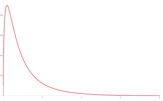
Figure 2: The density function for $Av(1342)$ constructed numerically, and a plot of the exact expression.

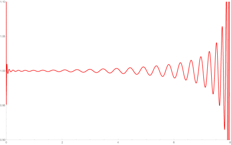
Figure 3: The ratio of the density function for $Av(1342)$ constructed numerically over the exact expression.

3 Increasing $Av(123\cdots(k+1))$ sequences

We apply the approach from the previous section, notably the Stieltjes inversion formula, to the explicit study of densities emerging from the classical “increasing subsequence problem”, or equivalently, from the study of permutations that avoid an increasing pattern of the form $(123\cdots(k+1))$.

Later, in Section 4, we address one of the most interesting unsolved problems in the area of pattern-avoiding permutations, that of enumerating permutations avoiding the pattern $(1324)$, by using a purely numerical approach to the Stieltjes inversion.

Let $\pi$ denote a permutation of $\{1,\ldots,n\}$. An increasing subsequence is a sequence $i_{1}<i_{2}<\cdots<i_{k}$ such that $\pi(i_{1})<\pi(i_{2})<\ldots<\pi(i_{k}).$ Let $f_{nk}$ denote the number of permutations $\pi$ with longest increasing subsequence of length at most $k$.

The number $\,f_{nk}$ is clearly identical to the number of permutations of $\{1,\ldots,n\}$ that avoid the pattern $(123\ldots(k+1))$; the set of these permutations is denoted by $Av_{n}(123\ldots(k+1))$, or simply by $Av(123\ldots(k+1))$, when the size $n$ is implicit.

In random matrix theory, a classical result of Diaconis and Shashahani [39] states that, if $U(k)$ represents the group of complex unitary matrices of size $k$, then

$$E_{M\in U(k)}\left(|\textrm{Tr}(M)|^{2n}\right)=n!\qquad\text{for}\;\;n\leqslant k.$$

Note that, in this context, the expectations are taken with respect to the Haar measure ${\mathbb{E}}(f):=\int_{M\in U(k)}f(M)dM$, where $\int$ is the Haar integral.

This result was extended to the case $n>k$ by Rains [104], who proved that

$$E_{M\in U(k)}\left(|\textrm{Tr}(M)|^{2n}\right)=\,f_{nk}.$$ (19)

From Rains’s result, we can deduce that for any $k$, the counting sequence $(f_{nk})_{n\in\mathbb{N}}$ of $Av(123\ldots k+1)$ is a Stieltjes moment sequence. To see this, let $X$ be a random variable with the same distribution as $|\textrm{Tr}(M)^{2}|_{M\in U(k)}$. Clearly $X$ is supported on the subset $[0,\,k^{2}]$ of $\mathbb{R}_{\geqslant 0}$; indeed, for a $k\times k$ unitary matrix $M$, $0\leqslant|\textrm{Tr}(M)|^{2}\leqslant k^{2}$, as each entry of the matrix has modulus $1$. Rains’s result implies that $f_{nk}$ is equal to the $n$-th moment ${\mathbb{E}}(X^{n})$ of the distribution of $X$. Hence $(f_{nk})_{n\in\mathbb{N}}$ is a Stieltjes moment sequence for any $k$. Moreover, the corresponding density function, that we will denote by $\mu_{k}(x)$, is precisely the density function of $|\textrm{Tr}(M)^{2}|_{M\in U(k)}$.

Equality (19) yields the following multiple integral representation for $f_{nk}$:

$$f_{nk}=\frac{1}{(2\pi)^{k}\,k!}\,\int_{[0,2\,\pi]^{k}}|e^{i\theta_{1}}+\cdots+e^{i\theta_{k}}|^{2n}\,\prod_{1\leqslant p<q\leqslant k}|e^{i\theta_{p}}-e^{i\theta_{q}}|^{2}\,d\theta_{1}\ldots d\theta_{k}.$$ (20)

In particular, the generating function for $Av(123\ldots(k+1))$ is D-finite, a result proved on the level of exponential generating functions and without using (20) by Gessel [55, p. 280]. Moreover, Bergeron and Gascon [15] explicitly computed the differential equations corresponding to the exponential generating functions for $k\leqslant 11$ (solving earlier conjectures made in [14]). Therefore, the results from the previous section imply that, for any $k$, the corresponding density $\mu_{k}(x)$ is also a D-finite function.

In subsequent subsections we explicitly find this density. In the simple case $k=\,2,$ this corresponds to the Catalan numbers, already treated in §2.5. For $k=\,3,\,4$ we calculate the density function $\mu_{k}(x)$ in terms of (pullbacks of) a rather special subset of ${}_{2}F_{1}$ hypergeometric functions corresponding to classical modular forms.

Note the formal resemblance of (20) with the multiple integral

$$W_{k}(n)=\frac{1}{(2\pi)^{k}}\,\int_{[0,2\,\pi]^{k}}|e^{i\theta_{1}}+\cdots+e^{i\theta_{k}}|^{2n}\,d\theta_{1}\ldots d\theta_{k}.$$ (21)

which occurs in the theory of uniform random walk integrals in the plane, where at each step a unit step is taken in a random direction [20, 21, 22]. The integral (21) expresses the $n$-th moment of the distance to the origin after $n$ steps. Of particular interest is the evaluation $W_{n}(1)$, which is equal to the expected distance after $n$ steps. We will actually see that there is a nontrivial link between the generating functions of $f_{nk}$ and of $W_{k}(n)$, mirrored by an equally nontrivial link between the corresponding densities $\mu_{k}(x)$ and $p_{k}(x)$.

The relationship between classical modular forms and some particular ${}_{2}F_{1}$ hypergeometric functions is discussed in a number of places in the literature (see for example [121], [82], [135]). One of the simplest illustrations of this intriguing relation can be seen in the identity [135, Eq. (74)]

$$E_{4}(q)={{}_{2}F_{1}}\left(\frac{1}{12},\frac{5}{12};1;\frac{1728}{j(q)}\right)^{4},$$ (22)

where $E_{4}(q)=1+240\,q+2160\,q^{2}+\cdots$ denotes the weight-four classical Eisenstein series, and where $j(q)=q^{-1}+744+196884\,q+21493760\,q^{2}+\cdots$ is the $j$-invariant (of an elliptic curve). In our examples, the Hauptmodul $1728/j$ will be a rational function $\mathcal{H}(x)$ of a variable $x$.

Modular forms (such as $E_{4}$) satisfy infinite order symmetries corresponding to the modular equations (see §3.2, or Appendix B and Appendix D). The pulled-back hypergeometric functions representing the classical modular forms (like ${{}_{2}F_{1}}\left(\frac{1}{12},\frac{5}{12};1;\mathcal{H}(x)\right)$) are annihilated by order-two linear differential operators. The corresponding nome $q(x)$ (explicitly, the exponential of the ratio of two solutions of the order-two operator) is a globally bounded series, i.e., it can be recast into a series with integer coefficients after a rescaling $x\rightarrow N\,x$.

The emergence of classical modular forms (closely associated with elliptic curves) in the density functions of $Av(1234)$ and $Av(12345)$ discussed below (§3.1 and §3.3), is a hint that the general $Av(123\ldots(k+1))$ series could be related to integrable theory, an observation which is in agreement with the relation with random matrix problems, discussed above.

For $k=5,\,6,\,7$, we construct explicitly a $(k-1)$-th order linear ODE for the density function $\mu_{k}(x)$ for $Av(123\ldots(k+1))$, and comment on its properties (§3.6, §3.8 and §3.9). These examples clearly demonstrate the procedure for the cases $k\geqslant 8.$

3.1 $Av(1234)$

The sequence $Av(1234)$ admits nice closed forms ([55, p. 281], [118, p. 12]),

$$f_{n3}\,=\,\sum_{k=0}^{n}{\frac{{2\,k\choose k}{n+1\choose k+1}{n+2\choose k+1}}{\left(n+1\right)^{2}\left(n+2\right)}}\,=\,2\,\sum_{k=0}^{n}{\frac{{2\,k\choose k}{n\choose k}^{2}\left(3\,{k}^{2}-2\,kn+2\,k-n+1\right)}{\left(k+1\right)^{2}\left(k+2\right)\left(n+1-k\right)}}.$$

Its generating function $F_{3}(x)$ starts

$$F_{3}(x)\,=\,1\,+x\,+2\,{x}^{2}\,+6\,{x}^{3}\,+23\,{x}^{4}\,+103\,{x}^{5}\,+513\,{x}^{6}\,+2761\,{x}^{7}\,+\,\,\cdots$$ (23)

and is a solution of an order-three operator $\,L_{3}\,=\,\,L_{1}\oplus\,L_{2}$ which is the direct sum of an order-one operator $\,L_{1}$ with a simple rational solution $\,{\cal R}(x)$ and an order-two linear differential operator $\,L_{2}$ (recall that $D_{x}$ denotes the derivation $\,d/dx$):

$$\quad\quad\quad L_{2}\,\,=\,\,\,\,D_{x}^{2}\,\,+\,\,{\frac{5\,-27\,x}{\left(1\,-9\,x\right)\,x}}\,\,D_{x}\,\,+\,{\frac{9\,{x}^{2}-9\,x+4}{x^{2}\,\,(1\,-9\,x)\,\,(1\,-x)}},$$ (24)

which can be shown to admit, as in [23], a pulled-back $\,{}_{2}F_{1}$ hypergeometric function $\,{\cal H}(x)$ as solution. Consequently, in a neighborhood of $x=0$, the series (23) can be written as the sum $F_{3}(x)\,=\,f_{1}\,:=\,{\cal R}(x)\,+\,{\cal H}(x)$, where:

$${\cal R}(x)\,=\,\,{{1\,+\,5\,x}\over{6\,x^{2}}},$$ (25)

$${\cal H}(x)=\,-\,{{(1\,-x)^{1/4}\,\,(1\,-9\,x)^{3/4}}\over{6\,x^{2}}}\,\,_{2}F_{1}\left(-\,{{1}\over{4}},\,{{3}\over{4}};\,1;\,\,{{-\,64\,x}\over{(1\,-x)\,\,(1\,-9\,x)^{3}}}\right)\!\!.$$ (26)

Note that the pulled-back $\,{}_{2}F_{1}$ hypergeometric $\,{\cal H}(x)$ is not a Taylor series but a Laurent series. The Taylor series with positive integer coefficients (23) amounts to getting rid of the poles of the Laurent series for $\,{\cal H}(x)$. Note that the pulled-back $\,{}_{2}F_{1}$ hypergeometric $\,{\cal H}(x)$ can also be rewritten using the identity

$$\quad{}_{2}F_{1}\left(-{{1}\over{4}},\,{{3}\over{4}};\,1;\,\,x\right)\,$$ (27)

$$\quad\,\,=\,\,\,(1\,-3\,x)\,\,_{2}F_{1}\left({{3}\over{4}},\,{{3}\over{4}};\,1;\,\,x\right)\,\,\,+\,4x\,(1\,-x)\,\,{{d\,}\over{dx}}\left(\,{}_{2}F_{1}\left({{3}\over{4}},\,{{3}\over{4}};\,1;\,\,x\right)\right),$$

as an order-one linear differential operator acting on a classical modular form since the $\,{}_{2}F_{1}$ pulled-back hypergeometric function ${}_{2}F_{1}\Bigl{(}{{3}\over{4}},\,{{3}\over{4}};\,1;\,\,x\Bigr{)}$ is actually a classical modular form, see (B.1) in [1, Appendix B] and Theorem 3 in [106], see also §3.2. Equation (70) in Appendix B also underlies a $\,x\,\leftrightarrow\,\frac{1}{9x}$ involutive symmetry for the pulled-back hypergeometric function $\,{\cal H}(x)$ and thus also for the $Av(1234)$ series (23).

3.2 Density of $Av(1234)$: Piecewise analysis

We recall that, for the sequence $f_{n3}$ for $\,Av(1234)$, the growth rate is $9$ [55, p. 280–281].

The general theory previously displayed tells us that the density can be obtained from formula (10), no matter whether the series we consider is an algebraic series, a D-finite series (as in this case $\,Av(1234)$), a differentially algebraic series, or a not-even-differentially algebraic series. Let us rewrite the Stieltjes inversion formula (10) giving the density as:

$$\quad\quad\quad\quad\mu_{3}(y)\,=\,\,-\frac{1}{\pi}\,\,\Im(\theta(y))\quad\quad\hbox{where:}\quad\quad\quad\theta(y)\,=\,\,{{1}\over{y}}\,\,F_{3}\Bigl{(}{{1}\over{y}}\Bigr{)}.$$ (28)

3.2.1 Naive approach

In the case of the $\,Av(1234)$ series (23), the function $\,\theta(y)$ is the sum of $\,1/y\cdot\,{\cal R}(1/y)$ and $\,\,1/y\cdot\,{\cal H}(1/y)$, which reads:

$$\quad\quad\theta(y)={{y+5}\over{6}}\,-\,\,{{(y-1)^{\frac{1}{4}}\,(y-9)^{\frac{3}{4}}}\over{6}}\,\,_{2}F_{1}\left(-{{1}\over{4}},\,{{3}\over{4}};\,1;\,\,-\,{{64\,y^{3}}\over{(y-1)\,(y-9)^{3}}}\right).$$ (29)

Since the imaginary part of a polynomial (such as $\,{{y+5}\over{6}}$) evaluated at real values is zero, it is clear that finding the imaginary part of (29) gives just the imaginary part of the pulled-back $\,{}_{2}F_{1}$ hypergeometric function $\,\,1/y\cdot\,{\cal H}(1/y)$. However evaluating the imaginary part of a pulled-back ${}_{2}F_{1}$ hypergeometric is not straightforward. This compels us to examine the function as a piecewise function.

The density $\,\mu_{3}(y)$ is defined on the interval $\,[0,\,9]$. We first note that the pullback in the pulled-back $\,{}_{2}F_{1}$ hypergeometric function in (29), is small when $\,y$ is small. Since we are dealing with $\,{}_{2}F_{1}$ hypergeometric functions we need to know, for $\,y\in\,[0,\,9]$ when the pullback $\,H\,=\,-\,{{64\,y^{3}}\over{(y-1)\,(y-9)^{3}}}$ satisfies $\,H\in\,(-\infty,\,0]$ or $\,H\in\,[0,\,1]$ or $\,H\in\,[1,\,\infty)$. This leads one to introduce the following intervals inside $\,[0,\,9]$: $[0,\,1]$, $[1,\,r]$, $[r,\,9]$, where $\,r$ is the algebraic number $\,r\,=\,6\sqrt{3}-9\,=\,1.39230485\ldots,$ and is a solution of the quadratic equation $\,y^{2}\,+18\,y\,-27\,=\,0$ corresponding to $\,H\,=\,1.$

The detailed piecewise analysis of this function and its imaginary part is given in Appendix A. The conclusion of this naive approach is that we find an expression which is the correct density, but divided by a factor of 3.

3.2.2 The magic of modularity

Actually, the origin of the factor 3 comes from the modular equation (B). More precisely, the following identity $\mathcal{H}(x)=\mathcal{H}_{2}(x)$ holds:

$$-\,{{(1\,-x)^{1/4}\,\,(1\,-9\,x)^{3/4}}\over{6\,x^{2}}}\,\,_{2}F_{1}\left(-\,{{1}\over{4}},\,{{3}\over{4}};\,1;\,\,{{-\,64\,x}\over{(1\,-x)\,\,(1\,-9\,x)^{3}}}\right)$$

$$=-\frac{(1-9x)^{1/4}\,(1+3x)^{2}}{6\,(1-x)^{5/4}\,x^{2}}\,\,\,_{2}F_{1}\left(-\,{{1}\over{4}},\,{{3}\over{4}};\,1;\,\,{{-\,64\,x^{3}}\over{(1\,-x)^{3}\,\,(1\,-9\,x)}}\right)$$

$$+\frac{32\,x^{3}\,(1-6x-3x^{2})}{27}\,\,\,_{2}F_{1}\left(-\,{{3}\over{4}},\,{{7}\over{4}};\,1;\,\,{{-\,64\,x^{3}}\over{(1\,-x)^{3}\,\,(1\,-9\,x)}}\right),$$ (30)

where $\mathcal{H}_{2}$ is the right-hand side of (3.2.2).

This expresses the fact that the principal part of the generating function of $Av(1234)$ corresponds to an order-one differential operator acting on a classical modular form.

Let us introduce $\mathcal{G}(y):=\frac{1}{y}\mathcal{H}(1/y)$ and $\mathcal{G}_{2}(y):=\frac{1}{y}\mathcal{H}_{2}(1/y)$. Naively, one could imagine that $\mathcal{G}(y)$ and $\mathcal{G}_{2}(y)$ are equal for small $y$ and possibly in some interval like $[0,9]$. In fact, this is not true: their series expansions around $y=0$ satisfy $3\,\mathcal{G}(y)=\mathcal{G}_{2}(y)$. In the Stieltjes inversion formula, the density candidate gets multiplied by a factor of 3. Thus, the corresponding density becomes the correct one.

3.2.3 Less naive approach

Again, we need to perform a piecewise analysis of the slightly more complicated expression $\mathcal{H}_{2}(y)$, as we did with $\mathcal{H}(y)$ in Appendix A. Not surprisingly, after performing this analysis, one gets the correct density. In Appendix C we sketch some arguments showing that this alternative expression $\mathcal{H}_{2}(y)$ behaves, as expected, better than the simpler one using $\mathcal{H}(y)$. In Fig. 4 we plot this correct density function, as well as plotting the density function, numerically constructed as described in Sec. 4.1. Again, they are graphically indistinguishable.

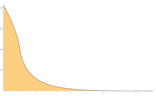
Figure 4: The density function $\mu_{3}(x)$ for $Av(1234)$ constructed numerically by a histogram (orange bars) and the plot created from the exact expression (blue curve). The plot also contains a polynomial approximation (red curve), but this is perfectly covered by the exact plot.

3.3 $Av(12345)$

The positive integer coefficient series $F_{4}(x)$ for $Av(12345)$ reads:

$$1\,+x\,+2\,{x}^{2}\,+6\,{x}^{3}\,+24\,{x}^{4}\,+119\,{x}^{5}\,+694\,{x}^{6}+4582\,{x}^{7}+33324\,{x}^{8}\,+\,\cdots$$ (31)

It is a solution of an order-four linear differential operator $\,L_{4}\,=\,\,L_{1}\,\oplus\,L_{3}$ which is the direct sum of an order-one linear differential operator $\,L_{1}$ with a simple rational solution $\,{\cal R}(x)=\frac{18\,{x}^{2}+10\,x+1}{12\,{x}^{3}}$ and an order-three linear differential operator $\,L_{3}$

$$\quad\quad L_{3}\,\,=\,\,D_{x}^{3}\,\,+{\frac{\left(448\,{x}^{2}-182\,x+13\right)}{x\,\,(1\,-16\,x)\,\,(1\,-4\,x)}}\,\,D_{x}^{2}$$

$$\quad\quad\quad\,\,\,\,\,\,+\,{\frac{4\,\,\left(160\,{x}^{2}-87\,x+11\right)}{{x}^{2}\,\,(1\,-16\,x)\,\,(1\,-4\,x)}}\,\,D_{x}\,\,\,+\,{\frac{4\,\,(32\,{x}^{2}-20\,x+9)}{(1\,-16\,x)\,\,(1\,-4\,x)\,\,{x}^{3}}},$$ (32)

which can be seen, using van Hoeij’s algorithm in [62], to be homomorphic (with order-two intertwiners) to the symmetric square of an order-two linear differential operator:

$$\,U_{2}\,\,=\,\,\,D_{x}^{2}\,\,\,+\,{\frac{2\,\,(32\,x\,-5)}{(1\,-16\,x)\,\,(1\,-4\,x)}}\,\,D_{x}\,\,\,+\,{\frac{1\,-8\,x}{4\,\,(1\,-16\,x)\,\,(1\,-4\,x)\,\,x^{2}}},$$ (33)

which has a classical modular form solution that can be written as a pulled-back hypergeometric function. In Appendix D we show that this pulled-back hypergeometric function is a classical modular form. Appendix D also underlines another involutive symmetry $\,x\,\leftrightarrow\,\frac{1}{64x}$ on this new classical modular form and thus on the $Av(12345)$ series (31).

Introducing $\,{\cal F}(x)\,=\,{\cal H}(x)^{2}$, the square of this classical modular form

$$\quad\quad\quad\,\,\,{\cal F}(x)\,\,=\,\,\,\,x\,\,(1\,-16\,x)^{-1/3}\,\,(1\,+2\,x)^{-2/3}$$

$$\quad\quad\quad\quad\quad\quad\quad\times\,\,_{2}F_{1}\left({{1}\over{6}},\,{{2}\over{3}};\,1;\,\,-\,{\frac{108\,{x}^{2}}{(1\,-16\,x)\,\,(1\,+2\,x)^{2}}}\right)^{2},$$ (34)

one finds that the series $F_{4}(x)$ for $\,Av(12345)$ can be written as the sum of the rational function $\,{\cal R}(x)$ (the solution of $\,L_{1}$) and an order-two linear differential operator acting on $\,{\cal F}(x)$ given by (3.3). Thus, the $\,Av(12345)$ series (31) is actually the expansion of

$$\quad-{\frac{\left(4\,x-1\right)\left(16\,x-1\right)\left(1376\,{x}^{2}+590\,x-1\right)}{864\,{x}^{3}}}\,\,{{d^{2}{\cal F}(x)}\over{dx^{2}}}$$

$$\quad\quad\quad\quad-{\frac{\left(63488\,{x}^{4}+10304\,{x}^{3}+396\,{x}^{2}-344\,x+1\right)}{864\,{x}^{4}}}\,\,{{d{\cal F}(x)}\over{d{x}}}$$ (35)

$$\quad\quad\quad\quad\quad\,\,-{\frac{\left(2176\,{x}^{3}-3372\,{x}^{2}+420\,x-1\right)}{864\,{x}^{5}}}\,\,{\cal F}(x)\,\,\,\,\,+{\frac{18\,{x}^{2}+10\,x+1}{12\,\,{x}^{3}}}.$$

Alternatively, $L_{3}$ can also be seen as being homomorphic (with order-two intertwiners) to the symmetric square of another order two linear differential operator, with a pulled-back hypergeometric solution:

$${}_{2}F_{1}\left({{1}\over{6}},\,{{1}\over{3}};\,1;\,\,\,{\frac{108\,{x}^{2}}{(1\,-4\,x)^{3}}}\right),$$

which emerges in the study of Domb numbers (counting $2n$-step polygons on the diamond lattice, and also the moments of a 4-step random walk in two dimensions, cf. https://oeis.org/A002895). In other words, the following identity holds:

$$\left(1-4\,x\right)^{\frac{1}{2}}\,\,_{2}F_{1}\left({{1}\over{6}},\,{{2}\over{3}};\,1;\,\,\,{\frac{-108\,{x}^{2}}{(1\,-16\,x)\,(1+2\,x)^{2}}}\right)$$

$$={\left(1-16\,x\right)^{\frac{1}{6}}\,\left(1+2\,x\right)^{\frac{1}{3}}}\,\,_{2}F_{1}\left({{1}\over{6}},\,{{1}\over{3}};\,1;\,\,\,{\frac{108\,{x}^{2}}{(1\,-4\,x)^{3}}}\right).$$ (36)

As we will see in the next subsection, the relation between the generating function $F_{4}(x)$ of $Av(12345)$ and the Domb generating function is not fortuitous: it mirrors what happens on the level of the density functions, namely that the density function $\mu_{4}(x)$ corresponding to $Av(12345)$ is intimately related to the density function $p_{4}(x)$ of the distance travelled in 4 steps by a uniform random walk in the plane [21].

3.4 Density of $Av(12345)$

The $Av(12345)$ density function $\mu_{4}(x)$ is also the probability density function of the squared norm of the trace of a random 4 by 4 unitary matrix. We recall that the support of the measure is $\,[0,\,16]$. The sequence (31) is a Stieltjes sequence, the density being given by the general formula (28). Again one has to change $\,x\,\rightarrow\,1/x$ in (3.3) and take the imaginary part of the slightly involved hypergeometric result.

As far as finding the density $\mu_{4}(x)$ is concerned (before undertaking the delicate piecewise analysis of taking the imaginary part) one finds, using (3.3) and Stieltjes inversion formula, that

$$\theta(x)=\frac{1}{x}\,\left(F_{4}\left(\frac{1}{x}\right)-\frac{1}{12}\,\left({x}^{2}+10\,x+18\right)x\right)$$

is equal to

$$\quad\quad\quad\theta(x)=x^{2}\,\,(4-x)\,\,(16-x)\,\,(x^{2}-590\,x-1376)\,\,{{d^{2}M(x)}\over{dx^{2}}}$$

$$\quad\quad\quad\quad\quad\,\,+\,x\,\,(3\,x^{4}-1564\,x^{3}+21372\,x^{2}-10176\,x-112640)\,\,{{dM(x)}\over{dx}}$$

$$\quad\quad\quad\quad\quad\,\,+x\,\,\left(x^{3}-420\,x^{2}+3372\,x-2176\right)\,\,M(x),$$ (37)

where:

$$\quad M(x)\,\,=\,\,\,(16\,-x)^{-1/3}\,\,(2\,+x)^{-2/3}\,\,_{2}F_{1}\left({{1}\over{6}},\,{{2}\over{3}};\,1;\,\,\,\,{\frac{108\,x}{(16\,-\,x)\,\,(2\,+\,x)^{2}}}\right)^{2}.$$

In this case the support of the measure $\mu_{4}(x)$ is $\,[0,\,16]$ and the piecewise analysis will need to consider the intervals $\,[0,\,4]$ and $\,[4,\,16]$. The value $\,4$ corresponds to the pullback $\,{\frac{108\,y}{(16\,-\,y)\,\,(2\,+\,y)^{2}}}$ being equal to $\,1$. We will not pursue these calculations in detail here, as they are similar to those in the previous section for $Av(1234)$. We simply show in Fig. 5 a plot of the density function $\mu_{4}(x)$ for $Av(12345)$ obtained numerically, using the approach described in §4.1.

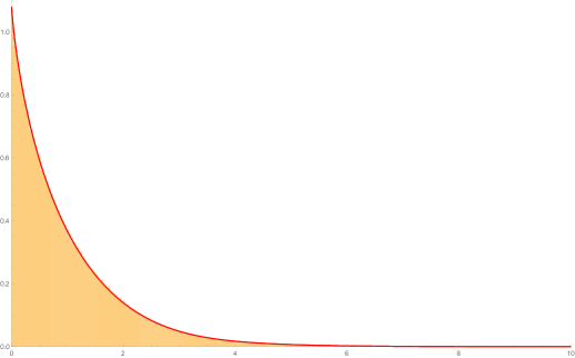
Figure 5: The density function $\mu_{4}(x)$ for $Av(12345)$ constructed numerically by a histogram (orange bars) and the polynomial approximation (red line).

The linear differential operator annihilating the density $\,\mu_{4}(x)$ is easily obtained from the pullback of the order-three operator $L_{3}$ in (3.3). It reads:

$$\left(x-4\right)\left(x-16\right)\,{x}^{2}D_{x}^{3}-2\,x\left(2\,{x}^{2}-x-64\right)D_{x}^{2}+10\,x\left(x+2\right)D_{x}-12\,(x-2).$$

Similarly, $\mu_{4}(x^{2})$ is a solution of the linear differential operator

$$\left(x^{2}-4\right)\,\left(x^{2}-16\right){x}^{2}D_{x}^{3}-\left(11\,{x}^{4}-64\,{x}^{2}-64\right)xD_{x}^{2}$$

$$+\left(51\,{x}^{4}+16\,{x}^{2}-64\right)D_{x}-96\,x\,\left({x}^{2}+2\right).$$ (38)

3.5 Relation between densities of $Av(12345)$ and of $4$-steps uniform random walks

An unexpectedly simple relation connects the density $\mu_{4}(x)$ for $Av(12345)$ and the density $p_{4}(x)$ of short uniform random walks studied in [21].

Recall that $p_{4}(x)$ denotes the density function of the distance travelled in $4$ steps by a uniform random walk in $\mathbb{Z}^{2}$ that starts at $(0,0)$ and consists of unit steps, each step being taken into a uniformly random direction. In [21, Thm. 4.7] it was shown that for $x\in(2,4)$,

$$p_{4}(x)=\frac{2}{\pi^{2}}\,\frac{\sqrt{4-x^{2}}}{x}\,\,_{3}F_{2}\left(\frac{1}{2},\,\frac{1}{2},\,\frac{1}{2};,\,\frac{5}{6},\,\frac{7}{6};\,\,\,{\frac{(16-x^{2})^{3}}{108\,x^{4}}}\right),$$

which satisfies the order-3 operator [21, Eq. (2.7)]

$$A_{4}=\left(x^{2}-4\right)\left(x^{2}-16\right){x}^{3}D_{x}^{3}+6\,{x}^{4}\left({x}^{2}-10\right)D_{x}^{2}+x\left(7\,{x}^{4}-32\,{x}^{2}+64\right)D_{x}+\left({x}^{4}-64\right).$$

Interestingly, the operator (3.4) satisfied by $\mu(x^{2})$ is gauge equivalent (homomorphic) with $A_{4}$, with a nontrivial order-2 intertwiner

$$x\left(x+4\right)\left(x-2\right)\left(x+2\right)\left(x-4\right)\left({x}^{4}-590\,{x}^{2}-1376\right)D_{x}^{2}$$

$$+\left(3\,{x}^{8}-1298\,{x}^{6}+11280\,{x}^{4}+10368\,{x}^{2}+38912\right)D_{x}$$

$$+{\frac{{x}^{8}-382\,{x}^{6}+2208\,{x}^{4}-19072\,{x}^{2}-38912}{x}}.$$ (39)

This shows that the density $p_{4}(x)$ and our density $\mu_{4}(x^{2})$, both with support $[0,4]$, are actually differentially related in a non-trivial way. More precisely, the operator (3.5) sends $p_{4}(x)$ to a solution of the operator (3.4) satisfied by $\mu_{4}(x^{2})$. Conversely, $\mu_{4}(x^{2})$ is mapped by a similar order-2 operator to a solution of the operator satisfied by $p_{4}(x)$.

We can push a bit further the analysis made in [21]. The operator $A_{4}$ annihilating $p_{4}(x)$ is the symmetric square of

$$4\left(x^{2}-4\right)\left(x^{2}-16\right)\,{x}^{2}D_{x}^{2}+8\,{x}^{3}\left({x}^{2}-10\right)D_{x}+({x}^{4}-12\,{x}^{2}+64),$$

which has a basis of solutions $\left\{y_{1}(x)=A(x)\,H_{1}(x),\;y_{2}(x)=A(x)\,H_{2}(x)\right\}$ with

$$H_{1}(x)=\;_{2}F_{1}\left({{1}\over{6}},\,{{2}\over{3}};\,1;\,\,\,\phi(x)\right),\quad H_{2}(x)=\;_{2}F_{1}\left({{1}\over{6}},\,{{2}\over{3}};\,\frac{5}{6};\,\,1-\,\phi(x)\right),$$

where

$$A(x)=\left(\frac{x^{3}}{(x^{2}+2)^{2}\,(16-x^{2})}\right)^{\frac{1}{6}}\qquad\text{and}\qquad\phi(x)={\frac{108\,{x}^{2}}{\left(16-x^{2}\right)\left({x}^{2}+2\right)^{2}}}.$$

Thus, $p_{4}(x)$ is equal to $c_{1}\,y_{1}(x)^{2}+c_{2}\,y_{2}(x)^{2}+c_{3}\,y_{1}(x)\,y_{2}(x),$ where

$$c_{1}={\frac{\sqrt{6}}{2\,\pi}},\quad\;c_{2}=\frac{2}{3}\,{\frac{\sqrt[6]{2}\,\pi\,\left(i-\sqrt{3}\right)}{\Gamma\left(2/3\right)^{6}}},\quad\;c_{3}=-\frac{2\,i}{3}{\frac{{2}^{5/6}\sqrt{3}}{\Gamma\left(2/3\right)^{3}}}.$$

Similarly, an explicit differential expression of order 2 in $\mu_{4}(x^{2})$ could also be written as a linear combination with constant coefficients of $y_{1}^{2},y_{2}^{2}$ and $y_{1}\,y_{2}$.

3.6 $Av(123456)$: order-four operator homomorphic to its adjoint

The positive integer coefficient series $F_{5}(x)$ for $Av(123456)$ reads:

$$1\,+x\,+2\,{x}^{2}\,+6\,{x}^{3}\,+24\,{x}^{4}\,+120\,{x}^{5}\,+719\,x^{6}\,+5003\,x^{7}\,+39429\,x^{8}\,+\,\cdots.$$ (40)

It is a solution of an order-five linear differential operator $\,L_{5}\,=\,\,L_{1}\,\oplus\,L_{4}$ which is the direct sum of an order-one operator $\,L_{1}$ with a simple rational solution $\,{\cal R}(x)$

$$\quad\quad\quad\quad\quad\quad{\cal R}(x)\,\,=\,\,\,\,\,{\frac{1\,+17\,x\,+71\,{x}^{2}+63\,{x}^{3}}{{20\,\,x}^{4}}},$$ (41)

and an order-four linear differential operator $\,L_{4}.$ This is

$$L_{4}=(x-1)\,(9\,x-1)\,(25\,x-1)\,x^{4}D_{x}^{4}+2x^{3}(1350x^{3}-1865x^{2}+336x-13)D_{x}^{3}$$

$$+x^{2}(8550x^{3}-14241x^{2}+3650x-215)D_{x}^{2}+x(7200x^{3}-14643x^{2}+5708x-649)D_{x}$$

$$+(900x^{3}-2325x^{2}+1225x-576).$$ (42)

The linear differential operator annihilating the corresponding density $\,\mu_{5}(x)$ can easily be obtained from the pullback of the order-four operator (3.6). Since we do not have any closed exact formula for its solutions we cannot perform the kind of piecewise analysis we performed previously. Mezzarobba’s algorithms [84] could in principle obtain (numerically) this density, by effective (numerical) analytic continuation.

The order-four operator $\,L_{4}$ is MUM (“maximal unipotent monodromy”) and is non-trivially homomorphic to its adjoint with an order-two intertwiner. Its exterior square has a rational solution of the form $\,P(x)/(301\,x^{11})$, where $\,P(x)$ is a polynomial with integer coefficients. The differential Galois group of the order-four operator $\,L_{4}$ is thus $\,Sp(4,\,\mathbb{C})$, or a special subgroup of it [28].

Remark. A priori, we cannot exclude the fact that $L_{4}$ could be homomorphic to the symmetric cube of a second-order linear differential operator, or to a symmetric product of two second-order operators. Furthermore, it could also be, in principle, that these second-order operators admit classical modular forms as solutions (pullbacks of special ${}_{2}F_{1}$ hypergeometric functions). However, these options can both be excluded by using some results from differential Galois theory [115], specifically from [100, Prop. 7, p. 50] for the symmetric cube case, and from [100, Prop. 10, p. 69] for the symmetric product case, see also [62, §3]. Indeed, if $L_{4}$ were either a symmetric cube or a symmetric product of order-two operators, then its symmetric square would contain a (direct) factor of order 3 or 1. This is ruled out by a factorization procedure which shows that the symmetric square of $L_{4}$ is (LCLM-)irreducible.

Still, we cannot exclude the fact that the solutions of $L_{4}$ (and in particular the generating function for $Av(123456)$, minus the rational part (41)) could be written as an algebraic pullback of a ${}_{4}F_{3}$ hypergeometric function.

We show in Fig. 6 a plot of the density function $\mu_{5}(x)$ for $Av(123456)$ obtained numerically, using the approaches described in §4.1. For $k>6$ we find that our approximations are visually indistinguishable from the graph of $e^{-x}$, so we do not display these plots separately.

Figure 6: The density function $\mu_{5}(x)$ for $Av(123456)$ constructed numerically by a histogram (orange bars) and the polynomial approximation (red line).

3.7 Relation between densities of $Av(123456)$ and of 5-steps uniform random walks

An unexpectedly simple relation connects the density $\mu_{5}(x)$ for $Av(123456)$ and the density $p_{5}(x)$ of short uniform random walks studied in [21].

Recall that $p_{5}(x)$ denotes the density function of the distance travelled in $5$ steps by a uniform random walk in $\mathbb{Z}^{2}$ that starts at $(0,0)$ and consists of unit steps, each step being taken into a uniformly random direction. In [21, Thm. 5.2] it was shown that for $x\in(0,5)\setminus\{1,3\}$, the density $p_{5}(x)$ satisfies the order-4 operator [21, Eq. (5.4)]

$$A_{5}=\left(x-1\right)\left(x-3\right)\left(x-5\right)\left(x+5\right)\left(x+3\right)\left(x+1\right){x}^{4}D_{x}^{4}$$

$$+2\,\left(5\,{x}^{6}-105\,{x}^{4}+259\,{x}^{2}+225\right)\,{x}^{3}D_{x}^{3}$$

$$+\left(25\,{x}^{6}-287\,{x}^{4}+363\,{x}^{2}-1125\right)\,{x}^{2}D_{x}^{2}$$

$$+\left(15\,{x}^{6}-77\,{x}^{4}-363\,{x}^{2}+2025\right)\,xD_{x}$$

$$+\left({x}^{6}-3\,{x}^{4}+363\,{x}^{2}-2025\right).$$

Interestingly, the operator satisfied by our density $\mu_{5}(x^{2})$,

$$-{x}^{3}\left(x-1\right)\left(x-3\right)\left(x-5\right)\left(x+5\right)\left(x+3\right)\left(x+1\right)D_{x}^{4}$$

$$+2\,{x}^{2}\left(13\,{x}^{6}-217\,{x}^{4}+363\,{x}^{2}+225\right)D_{x}^{3}$$

$$-x\left(287\,{x}^{6}-1685\,{x}^{4}-1323\,{x}^{2}+225\right)D_{x}^{2}$$

$$+\left(1575\,{x}^{6}-437\,{x}^{4}-1683\,{x}^{2}+225\right)D_{x}$$

$$-1200\,{x}^{3}\,\left(3\,{x}^{2}+5\right),$$ (43)

is gauge equivalent (homomorphic) with $A_{5}$, with a nontrivial order-3 intertwiner. This shows that the density $p_{5}(x)$ and our density $\mu_{5}(x^{2})$, both with support $[0,5]$, are actually differentially related in a non-trivial way. More precisely, the intertwiner sends $p_{5}(x)$ to a solution of the operator (43) satisfied by $\mu_{5}(x^{2})$. Conversely, $\mu_{5}(x^{2})$ is mapped by a similar order-2 operator to a solution of the operator satisfied by $p_{5}(x)$.

3.8 $Av(1234567)$: order-five operator homomorphic to its adjoint

The positive integer coefficient series $F_{6}(x)$ for $Av(1234567)$ reads:

$$1\,+x\,+2\,{x}^{2}\,+6\,{x}^{3}\,+24\,{x}^{4}\,+120\,{x}^{5}\,+720\,{x}^{6}\,\,+5039\,{x}^{7}\,+\,40270\,x^{8}\,+\,\,\cdots$$ (44)

It is a solution of an order-six linear differential operator $\,L_{6}\,=\,\,L_{1}\oplus\,L_{5}$ which is the direct sum of an order-one operator $\,L_{1}$ with a simple rational solution $\,{\cal R}(x)$

$$\quad\quad\quad\quad\quad\quad{\cal R}(x)\,\,=\,\,\,\,{\frac{1\,+26\,x\,+198\,x^{2}\,+476\,x^{3}\,+\,247\,x^{4}}{{30\,\,x}^{5}}}.$$ (45)

The linear differential operator $\,L_{5}$ is MUM and non-trivially homomorphic to its adjoint. The intertwiners have order 4. The symmetric square of $\,L_{5}$ has a rational solution of the form $\,P(x)/x^{N}$, where $\,P(x)$ is a polynomial. Its differential Galois group is thus a special subgroup of the orthogonal group $\,SO(5,\,{\mathbb{C}})$:

$$\qquad\qquad L_{5}=\,\left(4\,x-1\right)\,\left(16\,x-1\right)\,\left(36\,x-1\right)\,{x}^{5}\,D_{x}^{5}$$ (46)

$$+2\,\left(29376\,{x}^{3}-12232\,{x}^{2}+1106\,x-25\right){x}^{4}\,D_{x}^{4}$$

$$+2\,\left(241920\,{x}^{3}-124430\,{x}^{2}+14824\,x-449\right){x}^{3}\,D_{x}^{3}$$

$$+8\,\left(190944\,{x}^{3}-122397\,{x}^{2}+20161\,x-893\right){x}^{2}\,D_{x}^{2}$$

$$+4\,\left(425088\,{x}^{3}-343620\,{x}^{2}+82202\,x-6185\right)x\,D_{x}$$

$$+\,456192\,{x}^{3}-475344\,{x}^{2}+166912\,x-29160.$$

Once again, the operator satisfied by $\mu_{6}(x^{2})$ is gauge equivalent (homomorphic) with the operator $A_{6}$ satisfied by the density $p_{6}(x)$ in [21]. Therefore, $p_{6}(x)$ and our density $\mu_{6}(x^{2})$, both with support $[0,6]$, are actually differentially related in a non-trivial way.

3.9 $Av(12345678)$: order-six operator homomorphic to its adjoint

The positive integer coefficient series $F_{7}(x)$ for $Av(12345678)$ reads:

$$1+x+2\,{x}^{2}+6\,{x}^{3}+24\,{x}^{4}+120\,{x}^{5}+720\,{x}^{6}+5040\,{x}^{7}+40319\,{x}^{8}+362815\,{x}^{9}+\cdots$$

It is a solution of an order-seven linear differential operator $\,L_{7}\,=\,\,L_{1}\,\oplus\,L_{6}$ which is the direct sum of an order-one operator $\,L_{1}$ with a simple rational solution $\,{\cal R}(x)$

$$\quad\quad\mathcal{R}(x)\,\,=\,\,\,\,{\frac{1+37\,x+447\,{x}^{2}+2079\,{x}^{3}+3348\,{x}^{4}+1160\,{x}^{5}}{42\,\,{x}^{6}}},$$ (47)

and an order-six operator $L_{6}$,

$$L_{6}=\quad\left(x-1\right)\,\left(9\,x-1\right)\,\left(25\,x-1\right)\,\left(49\,x-1\right){x}^{6}D_{x}^{6}$$

$$+\left(297675\,{x}^{4}-434024\,{x}^{3}+85686\,{x}^{2}-4704\,x+71\right){x}^{5}D_{x}^{5}$$

$$+\left(2679075\,{x}^{4}-4858886\,{x}^{3}+1273932\,{x}^{2}-94818\,x+1913\right){x}^{4}D_{x}^{4}$$

$$+\,2\,\left(4862025\,{x}^{4}-10985516\,{x}^{3}+3929062\,{x}^{2}-424260\,x+12385\right){x}^{3}D_{x}^{3}$$

$$+\left(13693050\,{x}^{4}-38766996\,{x}^{3}+19376513\,{x}^{2}-3329230\,x+160367\right){x}^{2}D_{x}^{2}$$

$$+\left(5953500\,{x}^{4}-21425184\,{x}^{3}+15390947\,{x}^{2}-4684008\,x+483601\right)xD_{x}$$

$$+\,396900\,{x}^{4}-1887480\,{x}^{3}+2073337\,{x}^{2}-1002001\,x+518400.$$

The linear differential operator $\,L_{6}$ is non-trivially homomorphic to its adjoint. The intertwiners have order 4. Its differential Galois group is thus a special subgroup of the symplectic group $\,Sp(6,\,{\mathbb{C}})$.

As before, the operator satisfied by $\mu_{7}(x^{2})$ is gauge equivalent (homomorphic) with the operator $A_{7}$ satisfied by the density $p_{7}(x)$ in [21]. Therefore, $p_{7}(x)$ and our density $\mu_{7}(x^{2})$, both with support $[0,7]$, are actually differentially related in a non-trivial way.

3.10 $Av(1234{\ldots}(k+1))$: order-$(k-1)$ operator homomorphic to its adjoint

Recall that, by aforementioned results of Rains [104] and of Regev [105], the sequence $\,Av(1234{\ldots}{k+1})$ is a Stieltjes moment sequence with support $[0,k^{2}]$. Further, the generating function $F_{k}(x)$ of $Av(123\ldots(k+1))$ is D-finite, as proved by Gessel [55], see also [56, 92, 134]. More particularly, it belongs to the interesting subset of D-finite functions which can be written as diagonals of a rational function, as proved by Bousquet-Mélou [29, Prop. 13, p. 597]. It seems likely that many of the various remarkable properties enjoyed by the sequence $\,Av(1234{\ldots}(k+1))$ and by its generating function are consequences of these diagonal representations.

From all the examples of the previous subsections, it is legitimate to expect that for any $k$, the generating function $F_{k}(x)$ of $\,Av(1234{\ldots}(k+1))$ is a series solution of a linear differential operator $\,L_{k}(x,D_{x})\,$ of order $\,k$. The upper bound $k$ can be proven in the spirit of [15, Prop. 1]. It also appears that $\,L_{k}\,$ is moreover the direct sum $\,L_{k}\,=\,\,L_{1}^{(k)}\,\oplus\,L_{k-1}^{(k)}$ of an irreducible operator $L_{k-1}^{(k)}(x,D_{x})$ of order $k-1$ and of an order-one operator $L_{1}^{(k)}$ with a rational solution $\,{\cal R}_{k-2}(x)$ with a unique pole at $x=0$,

$$\quad\quad\quad\quad{\cal R}_{k-2}(x)\,\,=\,\,\,\,{\frac{P_{k-2}(x)}{k(k-1)\,\,{x}^{k\,-1}}},$$ (48)

where the polynomial $\,P_{k-2}(x)$ has degree $\,k\,-2$ and is of the form

$$P_{k-2}(x)\,=\,\,1\,+\,\cdots\,+\,c_{k-2}\,x^{k-2}.$$

Their coefficients are given in Table 1 for  $k\leqslant 10$. Note that they seem to have a very nice combinatorial interpretation: for fixed $r$, the sequence of coefficients $\left([x^{r}]\,P_{\ell}(x)\right)_{\ell\geqslant r+1}$ coincides with the sequence $\left(Q_{r}(\ell)\right)_{\ell\geqslant r+1}$ for some polynomial $Q_{r}(x)$ of degree $2r$ in $x$. For instance, when $r=1$, this sequence is $(\ell^{2}+1)_{\ell\geqslant 2}=(5,10,17,\ldots)$, and when $r=2$, this is $\left(\frac{1}{2}\,\ell^{4}-\ell^{3}+\frac{1}{2}\,\ell^{2}-\ell+3\right)_{\ell\geqslant 3}=(18,71,198,\ldots)$. Even more remarkably, the evaluation $Q_{r}(-d)$ of $Q_{r}(x)$ at negative integers $x=-d$ appears to count permutations of length $r+d$ that do contain an increasing subsequence of length $d$. In other words, the polynomials $Q_{r}(-d)$ are exactly the polynomials $B_{d}(d+r)$ of [41]. This surprising coincidence deserves a combinatorial explanation.

$\ell$ $\backslash$ $r$	0	1	2	3	4	5	6	7
2	1	5
3	1	10	18
4	1	17	71	63
5	1	26	198	476	247
6	1	37	447	2079	3348	1160
7	1	50	878	6668	21726	25740	6588
8	1	65	1563	17539	95339	235755	218844	44352

Table 1: Coefficients of $x^{d}$ in the numerators $P_{\ell}(x)$ of $\mathcal{R}_{\ell}(x)$, for $\ell\leqslant 8$.

The order-$(k-1)$ linear differential operator $\,L_{k-1}^{(k)}$ appears to be Fuchsian, MUM and homomorphic to its adjoint. As a consequence of this, it has a differential Galois group which is a subgroup of the orthogonal group $\,SO(k-1,\,{\mathbb{C}})$ when $k$ is even, and of the symplectic group $\,Sp(k-1,\,{\mathbb{C}})$ when $k$ is odd.

The linear differential operator $\,L_{k-1}^{(k)}$ has a Laurent series solution $\,\ell_{k-1}(x)$ whose sum with the Laurent series expansion of the rational function $\,{\cal R}_{k-2}(x)$ is exactly the generating function $F_{k}(x)$ of $Av(1234{\ldots}(k+1))$:

$$\quad\quad\quad\quad\ell_{k-1}(x)\,+\,{\cal R}_{k-2}(x)\,\,=\,\,\,\,1\,+x\,+2\,{x}^{2}\,+6\,{x}^{3}\,+24\,{x}^{4}\,+\,\,\cdots.$$ (49)

Therefore, the explicit calculation of the density function $\mu_{k}(x)$ for the Stieltjes sequence $Av(1234{\ldots}(k+1))$ amounts to performing a piecewise analysis of the sum

$$\quad\quad\quad\quad\quad\quad\quad-{{1}\over{\pi y}}\,\,\ell_{k-1}\Bigl{(}{{1}\over{y}}\Bigr{)}\,\,-{{1}\over{\pi y}}\,\,{\cal R}_{k-2}\Bigl{(}{{1}\over{y}}\Bigr{)}.$$ (50)

Because of the special form of ${\cal R}_{k-2}(x)$, the function $\,1/y\cdot{\cal R}_{k-2}(1/y)$ is a polynomial. The imaginary part of the evaluation of this polynomial for real values of $\,y$ is zero. The density function for the Stieltjes sequence $Av(1234{\ldots}(k+1))$ is thus a piecewise D-finite function, and a solution of the order-$(k-1)$ linear differential operator

$$\quad\quad\quad\quad\quad\quad\quad\quad pullback\Bigl{(}L_{k-1}^{(k)},\,{{1}\over{y}}\Bigr{)}\,\,y.$$ (51)

Of course, this linear differential operator is again (non-trivially) homomorphic to its adjoint, and it has the same differential Galois group as $\,L_{k-1}^{(k)}$.

Remark. For $k\geqslant 5$, we exclude the fact that $L_{k-1}^{(k)}$ could be homomorphic to the $(k-2)$-th power of a second-order linear differential operator. However, we cannot exclude the fact that the solutions of $L_{k-1}^{(k)}$, and in particular the generating function $F_{k}(x)$ of $Av(12\ldots(k+1))$, minus the rational part $\,{\cal R}_{k-2}(x)$ in (48), could be written as an algebraic pullback of a ${}_{k-1}F_{k-2}$ hypergeometric function. If we were forced to make a bet, our guess would be that the solutions might belong to the world of (specializations of) multivariate hypergeometric functions.

3.11 The double Borel transform of the $Av(123\ldots(k+1))$ sequences

Another explicit study of the generating functions for the $Av(123\ldots(k+1))$ sequences was undertaken by Bergeron and Gascon [15].

In 1990 Gessel [55] had shown that the double Borel transform of the generating function of $Av(123\ldots(k+1))$ could be expressed as the determinant of a $k\times k$ matrix whose coefficients are Bessel functions. More precisely, recalling that the generating function of $Av(123\ldots(k+1))$ is $\sum_{n}f_{nk}\,x^{n},$ with $f_{nk}$ as in (19) and (20), then the double Borel transform

$$Y_{k}(x)=\sum_{n\geqslant 0}\frac{f_{nk}}{n!^{2}}\,x^{n}$$

is equal to the determinant of the Toeplitz matrix $\displaystyle{[I_{i-j}(x)]_{1\leqslant i,j\leqslant k}},$ where

$$I_{k}(x)=\sum_{n=0}^{\infty}\frac{x^{n+k/2}}{n!(n+k)!}.$$

Clearly, for fixed $k$, the power series $I_{k}(x)$ is D-finite, so an immediate consequence of Gessel’s result is that $Y_{k}(x)$ is also D-finite. Bergeron and Gascon [15] showed that, moreover, $Y_{k}(x)$ can be expressed as homogeneous polynomials in the D-finite functions $I_{0}(x)$ and $I_{1}(x)$

$$I_{0}(x)=1+x+{\frac{1}{4}}{x}^{2}+{\frac{1}{36}}{x}^{3}+{\frac{1}{576}}{x}^{4}+\cdots,\quad I_{1}(x)=\sqrt{x}\,\left(1+{\frac{1}{2}}x+{\frac{1}{12}}{x}^{2}+{\frac{1}{144}}{x}^{3}+\cdots\right)$$

satisfying the order-two linear differential equations

$$xI_{0}^{\prime\prime}(x)+I_{0}^{\prime}(x)-I_{0}(x)=0\quad\text{and}\quad 4\,{x}^{2}I_{1}^{\prime\prime}(x)+4\,xI_{1}^{\prime}(x)-\left(4\,x+1\right)I_{1}(x)=0.$$ (52)

For instance,

$$Y_{2}=I_{0}(x)^{2}-I_{1}(x)^{2}\quad\text{and}\quad Y_{3}={\frac{2\,\sqrt{x}I_{0}(x)^{2}I_{1}(x)-I_{0}(x)\,I_{1}(x)^{2}-2\,\sqrt{x}I_{1}(x)^{3}}{x}}.$$

The underlying differential operators $\mathcal{L}_{2}(x),\,\mathcal{L}_{3}(x),\,\ldots,\,\mathcal{L}_{7}(x)$ for $Y_{2}(x),\,Y_{3}(x),\,\ldots,\,Y_{7}(x)$ were derived Bergeron and Gascon in [15]. For instance,

$$\mathcal{L}_{2}={x}^{2}D_{x}^{3}+4\,xD_{x}^{2}-2\,\left(2\,x-1\right){\it D_{x}}-2$$

and

$$\mathcal{L}_{3}={x}^{3}D_{x}^{4}+10\,{x}^{2}D_{x}^{3}-x\left(10\,x-23\right)D_{x}^{2}-\left(32\,x-9\right)D_{x}+9\,x-9.$$

The solutions of the differential equations $\mathcal{L}_{k}(y(x))=0$ are not given by regular hypergeometric functions or solutions of Fuchsian linear differential operators, but rather by solutions of linear differential operators with an irregular singularity at $\,\infty.$ The differential operators $\mathcal{L}_{k}$ are again homomorphic to their adjoint. Moreover, since the operators (52) are homomorphic and the $Y_{k}$ are homogeneous polynomials in $I_{0}$ and $I_{1}$, one deduces immediately that the $\mathcal{L}_{k}$’s are homomorphic to the $k$-th symmetric power of the order two operator $\mathcal{L}_{1}=xD_{x}^{2}+D_{x}-1$.

It is known [32] that symmetric powers of a fixed second-order operator are related by a recurrence of order two with simple order-1 operators as coefficients: if $\mathcal{M}=D_{x}^{2}+a(x)D_{x}+b(x)$, and then its $n$-th symmetric power is given by the $n$-th term of the sequence of operators

$$\mathcal{M}_{0}=1,\quad\mathcal{L}_{1}=D_{x},\quad\text{and for all }\;\;k\geqslant 1,$$

$$\mathcal{M}_{k+1}=(D_{x}+k\cdot a(x))\cdot\mathcal{M}_{k}+k(n-k+1)\cdot b(x)\cdot\mathcal{M}_{k-1}.$$ (53)

Our operators $\mathcal{L}_{k}$ are not symmetric powers, but are homomorphic to such symmetric powers. Consequently, we do not expect a recurrence as simple as the one on the $\mathcal{M}_{k}$’s. However, we remark that the $\mathcal{L}_{k}$’s still possess some remarkable features. For instance,

$$\mathcal{L}_{k+1}=\left(xD_{x}+\binom{k}{2}+1\right)\cdot\mathcal{L}_{k}$$

$$+\left(\binom{k+1}{4}-\binom{k+1}{2}x\right)\cdot\mathcal{L}_{k-1}\,+\,\left(\text{terms of ord}\;\leqslant k-2\right).$$ (54)

By analogy with the emergence of these symmetric powers for $\mathcal{L}_{k}$, one could imagine that the $L_{k}$’s associated with $Av(12\ldots(k+2))$ might also be homomorphic to the symmetric $(k-1)$-th power of an order 2 differential operator, which would hopefully correspond to a classical modular form.

4 A difficult case: $Av(1324)$

In this section, we investigate the density function for the most difficult Wilf class of length-4 pattern-avoiding permutations, namely $Av(1324),$ whose generating function is unknown. The study of this (conjectured) density function is entirely numerical, based on the extensive exact enumerations of Conway, Guttmann and Zinn-Justin [38].

The series with positive integer coefficients for $Av(1324)$ is

$$1+x+2\,x^{2}+6\,x^{3}+23\,x^{4}+103\,x^{5}+513\,x^{6}+2762\,x^{7}+15793\,x^{8}+\ldots,$$

and is known [38] up to order $x^{50}.$ The generating function is not known, and there are compelling arguments [38] that it is not D-finite. While it is known that the coefficients grow exponentially as $\lambda^{n},$ the value of $\lambda$ is not known. The best estimate is in [38] and is $\lambda=11.60\pm 0.01.$ The best rigorous bounds [16] are $10.27<\lambda<13.5$, while the paper [36] gives the improved upper bound $e^{\pi\,\sqrt{2/3}}\approx 13.001954$, but only under a certain conjecture about the number of inversions in a 1324-avoiding permutation.

The Hankel determinants are all positive and are monotonically increasing, which provides strong evidence for the conjecture that the series is a Stieltjes moment sequence.

Recall that if the sequence ${\bf a}$ is positive, then its log-convexity implies that the coefficient ratios $\frac{a_{n}}{a_{n-1}}$ are lower bounds on the growth rate $\mu$ of the sequence. In this way we obtain $\lambda>9.03.$

In the case that ${\bf a}$ is a Stieltjes moment sequence, stronger lower bounds for $\mu$ can be calculated using a method first given by Haagerup, Haagerup and Ramirez-Solano [59], that we now summarize.

Using the coefficients $a_{0},a_{1},\ldots\,a_{n},$ one calculates the terms $\,\alpha_{0},\alpha_{1},\ldots\alpha_{n}$ in the continued fraction representation given in Theorem 1. It is easy to see that the coefficients of $A(x)$ are nondecreasing in each $\alpha_{j}.$ Hence $A(x)$ is (coefficient-wise) bounded below by the generating function $A_{n}(x)$, defined by setting $\,\alpha_{n},\alpha_{n+1},\,\alpha_{n+2}\,\ldots,$ to 0. Therefore, the growth rate $\mu_{n}$ of $A_{n}(x)$ is not greater than the growth rate $\mu$ of $A(x).$ The growth rates $\,\mu_{1},\,\mu_{2},\,\ldots$ clearly form a non-decreasing sequence, and, since the coefficients of $A_{n}(x)$ are log-convex, $\mu_{n}\geqslant a_{n}/a_{n-1}$. It follows that this sequence $\,\mu_{1},\,\mu_{2},\,\ldots$ of lower bounds converges to the exponential growth rate $\mu$ of a.

If we assume further that the sequences $\,\alpha_{0},\,\alpha_{2},\,\alpha_{4}\,\ldots$ and $\alpha_{1},\alpha_{3},\alpha_{5}\ldots$ are non-decreasing, as we find empirically in many of the cases we consider, we can get stronger lower bounds for the growth rate by setting $\,\alpha_{n+1},\,\alpha_{n+3}\,\ldots$ to $\,\alpha_{n-1}$ and $\,\alpha_{n+2},\,\alpha_{n+4}\,\ldots$ to $\alpha_{n}$. For this sequence the exponential growth rate of the corresponding sequence ${\bf a}$ is $(\sqrt{\alpha_{n}}\,+\sqrt{\alpha_{n-1}})^{2}.$ By the method with which we constructed this bound, it is clear that $(\sqrt{\alpha_{n}}\,+\sqrt{\alpha_{n-1}})^{2}\geqslant\mu_{n}.$ Hence, the lower bounds $(\sqrt{\alpha_{n}}\,+\sqrt{\alpha_{n-1}})^{2}$ converge to the growth rate $\mu.$

In particular, if $\alpha_{n}\leqslant\alpha_{n+2}$ for each $n$ and the limit $\lim_{n\to\infty}\alpha_{n}$ exists, then it is equal to $\mu/4.$ Extensive use of this result in studying the cogrowth sequences of various groups has been made in [59] and [43]. A plot of the known values of $\alpha_{n}$ for $Av(1324)$ is shown in Fig. 7.

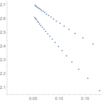
Figure 7: Plot of $\alpha_{n}$ (vertical axis) against $n^{-2/3}$ (horizontal axis) for the sequence $Av(1324)$ using coefficients $10\ldots 50$.

It appears that the coefficients $\alpha_{2k}$ and the coefficients $\alpha_{2k+1}$ each form an increasing sequence which is roughly linear when plotted against $n^{-2/3}.$ If this trend continues, the terms $\alpha_{n}$ will certainly all be positive. If it could be proved that this is a Stieltjes moment sequence, these $\alpha$ values would imply a lower bound of $\lambda>10.302,$ which is an improvement on the best lower bound cited above. If we assume further that the sequences $(\alpha_{2k})_{k\geqslant 0}$ and $(\alpha_{2k+1})_{k\geqslant 0}$ are both increasing, we get an improved lower bound $\lambda>10.607.$

Extrapolating the two subsequences $(\alpha_{2k})_{k\geqslant 0}$ and $(\alpha_{2k+1})_{k\geqslant 0}$, it seems plausible that these both converge to the same constant $c\approx 2.9,$ which is consistent with the growth rate $\lambda\approx 11.60$ predicted by Conway, Guttmann and Zinn-Justin [38].

From the numerical data, a histogram of the density function can be constructed, and this is shown in Fig. 8. We have no explanation for the little wiggle near the origin.

4.1 Numerics

We have used two different types of numerical construction of the density functions.

The histogram for $Av(12\ldots k)$ (D-finite, discussed in §3.1) is constructed as follows:

• take a random $(k-1)\times(k-1)$ matrix with entries which independently have standard complex normal distributions

• orthogonalize it to create a random unitary matrix

• compute the norm of the trace squared (by the Rains result [104] the $n$-th moment of this distribution is exactly the number of $12\ldots k$-avoiding permutations of size $n$)

• repeat the above steps $500\,000$ times and draw a histogram of the results, where each bar has width $0.02$

Note that this procedure does not use the exact coefficients.

The polynomial approximations for the densities are constructed by computing the moments $a_{0},a_{1},\ldots,a_{n}$ (that is, just the initial terms of the sequence), then approximating the density function by the unique polynomial $P(t)$ of degree $n+2$ over the known range $[0,\mu)$ with the following properties:

• the initial moments of the distribution with density $P(t)$ are $a_{0},a_{1},\ldots,a_{n}$

• $P(\mu)=P^{\prime}(\mu)=0$

For $Av(1342)$, we have $\mu=8$. For $Av(1324)$ we chose $\mu=12$, though for any value of $\mu$ between 11 and 13 the figure looks almost identical.

4.2 Final remarks

Remark 1. For each permutation $\pi$ of length at most $4$, we have proved or given strong evidence that the sequence $\big{(}Av_{n}(\pi)\big{)}_{n\geqslant 0}$, whose general term is the number of permutations of $\{1,\ldots,n\}$ that avoid the pattern $\pi$, is a Stieltjes moment sequence. Indeed, there is only one Wilf class of length 3, namely $(123)$, considered in §2.5 and there are 3 Wilf classes of length 4, namely $(1342),(1234)$ and $(1324)$. We proved that the first three are Stieltjes moment sequences (in §2.5, §2.6 and §3.1) and presented numerical evidence (in §4.1) for the last one. Moreover, the same equally holds for any $\pi$ of the form $(12\ldots k)$, as showed in §3. This naturally suggests the further question:

Open question: Is it the case that, for every permutation $\pi$, the sequence $\big{(}Av_{n}(\pi)\big{)}_{n\geqslant 0}$ is a Stieltjes moment sequence?

We tested all known terms of these sequences and found they are consistent with being Stieltjes moment sequences. However, to our knowledge, substantial computations of the initial terms of these sequences have only been done in the cases discussed in our paper.

Remark 2. One of the referees suggested that the classes of triples and pairs of length-4 pattern-avoiding permutations enumerated by Albert et al. [4], and conjectured to be non-D-finite, should be similarly studied. These sequences are $Av(4123,4231,4312)$, $Av(4123,4231)$, $Av(4123,4312)$ and $Av(4231,4321)$, and their first terms are given in the OEIS as A257562, A165542, A165545, A053617, respectively. Unfortunately, they all have Hankel determinants that become negative after a certain order, and so cannot be described as Stieltjes moment sequences.

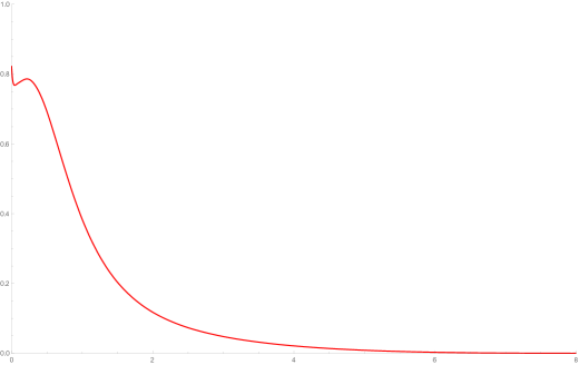
Figure 8: The density function for $Av(1324)$ constructed numerically.

5 Conclusion

We have shown how considering coefficients of combinatorial sequences as moments of a density function can be useful. Quite often in the literature the analysis of Stieltjes moment sequences with explicit densities is performed only for algebraic series which are slightly over-simplified degenerate cases.

We have studied here in some detail examples that are not algebraic series. For instance we have shown that $\,Av(1234)$ is a Stieltjes sequence whose generating function corresponds, up to a simple rational function, to an order-one linear differential operator acting on a classical modular form represented as a pulled-back $\,{}_{2}F_{1}$ hypergeometric function, and $\,Av(12345)$ is a Stieltjes sequence whose generating function, up to a simple rational function, corresponds to an order-two linear differential operator acting on the square of a classical modular form represented as a pulled-back $\,{}_{2}F_{1}$ hypergeometric function. The corresponding densities are of the same type, and do not involve the rational function. This scheme generalizes to all the $\,Av(12345\dots k)$ which are all Stieltjes moment sequences.

The linear differential operators annihilating such series are direct sums of an order-one operator with a simple rational solution where the denominator is just a power of $\,x$, and a linear differential operator homomorphic to its adjoint (thus corresponding to selected differential Galois groups). This last operator has a Laurent series solution, the generating function of the Stieltjes sequence corresponding to getting rid of the finite number of poles. The density is the solution of the $\,x\,\rightarrow\,1/x$ pullback of this last operator, but finding the actual density requires delicate piecewise analysis which is difficult to perform when one does not have exact expressions for the generating function of the Stieltjes moment sequence.

We have shown that the density function for the Stieltjes moment sequence $Av(12\ldots k)$ is closely, but non-trivially, related to the density attached to the distance traveled by a walk in the plane with $k-1$ unit steps in random directions.

Finally, we have considered the challenging (and still unsolved!) case of $Av(1324)$, and provided compelling numerical evidence that the corresponding counting sequence is a Stieltjes sequence. Assuming this, we obtained lower bounds to the growth constant that are better than existing rigorous bounds.

Acknowledgments. We thank the referees for their very careful reading and for providing many useful and constructive suggestions. Jean-Marie Maillard thanks The School of Mathematics and Statistics, The University of Melbourne, Australia, where part of this work has been performed. Alin Bostan and Jean-Marie Maillard address their warm thanks to the Café du Nord (Paris, France) where they had the chance to work daily during the massive French pension reform strike (December 2019). Alin Bostan has been supported by DeRerumNatura ANR-19-CE40-0018. Andrew Elvey Price has been supported by European Research Council (ERC) under the European Union’s Horizon 2020 research and innovation programme under the Grant Agreement No. 759702. Anthony John Guttmann wishes to thank the ARC Centre of Excellence for Mathematical and Statistical Frontiers (ACEMS) for support.

Appendix A Density of $Av(1234)$: Piecewise analysis

Discussion of the evaluation of $\,{}_{2}F_{1}$ in Maple

As far as the evaluation of a Gauss hypergeometric series like $\,{}_{2}F_{1}(-1/4,3/4;\,1;\,H)$ goes, the hypergeometric series converges for $\,|H|<1$, and $\,{}_{2}F_{1}(a,b;\,c,\,H)$ is then defined for $\,|H|\geqslant\,1$ by analytic continuation. The point $z=1$ is a branch point, and the interval $[1,\,\infty]$ is the branch cut, with the evaluation on this cut taking the limit from below the cut. We need to look at [63, 64, 11]. The hypergeometric function $\,{}_{2}F_{1}(a,b;\,c;\,H)$ can be rewritten using the Pfaff connection formulas:

$$\quad\quad\quad{}_{2}F_{1}(a,\,b;\,c;\,H)\,\,\,\,=\,\,\,\,(1\,-H)^{-a}\,\,_{2}F_{1}\Bigl{(}a,\,c\,-b;\,c;\,\,-\,{{H}\over{1\,-H}}\Bigr{)}$$

$$\quad\quad\quad\quad\quad\quad\quad\quad\quad\,\,=\,\,\,(1\,-H)^{-b}\,\,_{2}F_{1}\Bigl{(}c\,-a,\,b;\,c;\,\,-\,{{H}\over{1\,-H}}\Bigr{)}.$$ (55)

These formulas enable one to evaluate $\,{}_{2}F_{1}(-1/4,3/4;\,1;\,H)$ for negative real values of $\,H$, changing them to the evaluation of $\,{}_{2}F_{1}(3/4,5/4;\,1;\,\tilde{H})$ or $\,{}_{2}F_{1}(-1/4,1/4;\,1;\,\tilde{H})$ with $\,\tilde{H}\,\in\,[0,\,1]$. In our case this gives for $\,H\,<\,0$:

$$\quad\quad\,{}_{2}F_{1}\Bigl{(}-{{1}\over{4}},{{3}\over{4}};\,1;\,H\Bigr{)}\,\,\,=\,\,\,\,(1\,-H)^{1/4}\,\,_{2}F_{1}\Bigl{(}-{{1}\over{4}},\,{{1}\over{4}};\,1;\,\,-\,{{H}\over{1\,-H}}\Bigr{)},$$ (56)

which corresponds to real positive values.

To evaluate $\,{}_{2}F_{1}(-1/4,3/4;\,1;\,H)$ for positive real values of $\,H$ larger than $\ 1$ with ($H\in(1,\,\infty]$), we must use the connection formula 15.10.21 in https://dlmf.nist.gov/15.10#E21 (see [63, 64, 11]):

$$\quad\quad{}_{2}F_{1}\Bigl{(}a,\,b;\,c;\,H\Bigr{)}\,\,=\,\,\,{{\Gamma(a)\,\Gamma(b)}\over{\Gamma(c-a)\,\Gamma(c-b)}}\,\,w_{3}\,\,\,+{{\Gamma(c)\,\Gamma(a+b-c)}\over{\Gamma(a)\,\Gamma(b)}}\,\,w_{4},$$ (57)

where $\,w_{3}$ is alternatively one of the two formulas:

$$\quad\quad\quad\,w_{3}\,\,=\,\,\,_{2}F_{1}\Bigl{(}a,\,b;\,a\,+b\,-c+1;\,1\,-\,H\Bigr{)},$$

$$\quad\quad\quad\quad\quad\,\,\,=\,\,\,H^{-a}\,\,_{2}F_{1}\Bigl{(}a,\,a\,-c\,+1;\,a\,+b\,-c+1;\,1\,-\,{{1}\over{H}}\Bigr{)},$$ (58)

and $\,w_{4}$ is alternatively one of the two formulas:

$$\quad\,w_{4}\,\,=\,\,\,\,\,(1\,-H)^{c-a-b}\,\,_{2}F_{1}\Bigl{(}c\,-a,\,c\,-b;\,c\,-a\,-b+1;\,1\,-\,H\Bigr{)}$$ (59)

$$\quad\quad\,\,\,=\,\,\,\,H^{a-c}\,\,(1\,-H)^{c-a-b}\,\,_{2}F_{1}\Bigl{(}c\,-a,\,1\,-a;\,c\,-a\,-b\,+1;\,1\,-\,{{1}\over{H}}\Bigr{)}.$$

In our case this gives for $\,H\,>\,1$:

$$\quad\quad\,{}_{2}F_{1}\Bigl{(}-{{1}\over{4}},{{3}\over{4}};\,1;\,H\Bigr{)}\,\,\,=\,\,\,\,{{2\,\Gamma(3/4)^{2}}\over{\pi^{3/2}}}\,\,H^{1/4}\,\,_{2}F_{1}\Bigl{(}-{{1}\over{4}},\,-{{1}\over{4}};\,{{1}\over{2}};\,1\,-\,{{1}\over{H}}\Bigr{)}$$

$$\quad\quad\quad\quad\quad\,\,\,+{{\pi^{1/2}}\over{2\,\Gamma(3/4)^{2}}}\,\,H^{-5/4}\,\,(1\,-H)^{1/2}\,\,_{2}F_{1}\Bigl{(}{{5}\over{4}},\,{{5}\over{4}};\,{{3}\over{2}};\,1\,-\,{{1}\over{H}}\Bigr{)}.$$ (60)

For $\,H\,>\,1$, that the first term on the RHS of (A) corresponds to positive real values while the second term on the RHS of (A) corresponds to purely imaginary values:

$$\quad\quad\,\Im\Bigl{(}\,_{2}F_{1}\Bigl{(}-{{1}\over{4}},{{3}\over{4}};\,1;\,H\Bigr{)}\Bigr{)}$$

$$\quad\quad\quad\quad\,\,\,\,=\,\,\,\,{{\pi^{1/2}}\over{2\,\Gamma(3/4)^{2}}}\,\,H^{-5/4}\,\,(H\,-1)^{1/2}\,\,_{2}F_{1}\Bigl{(}{{5}\over{4}},\,{{5}\over{4}};\,{{3}\over{2}};\,1\,-\,{{1}\over{H}}\Bigr{)}.$$ (61)

See equation 15.10.21 in https://dlmf.nist.gov/15.10#E21

Note that both Maple and Mathematica compute these by defining $\,{}_{2}F_{1}(a,b;c;z)$ to be analytic in $z$ except on the cut $\,[1,\infty]$, and, on this cut, they both take the limit from below the cut.

The piecewise analysis

For $\,y\,\in\,\,[0,\,1]$ the pullback gives $\,H\,\in\,\,(-\infty,\,0]$, so $\,{}_{2}F_{1}\Bigl{(}-{{1}\over{4}},\,{{3}\over{4}};\,1;\,\,H\Bigr{)}\,\in\,\,[1,\,\infty]$.

For $\,y\,\in\,\,[1,\,6\sqrt{3}-9]$ the pullback gives $\,H\,\in\,\,[1,\,\infty]$. For $\,y\,\in\,\,[6\sqrt{3}-9,\,9]$ the pullback also gives $\,H\,\in\,\,[1,\,\infty]$. Since the imaginary part of a polynomial (such as $\,{{y+5}\over{6}}$) evaluated at real values is zero, the imaginary part of (29) is the imaginary part of the pulled-back hypergeometric term in (29) which reads:

$\,\bullet$ For $\,y\,\in\,[0,\,1]$ (i.e. $\,H\,\in\,[-\infty,\,0]$), and ${}_{2}F_{1}(-1/4,3/4;\,1;\,H)$ is given by (56) and is real and positive), the imaginary part of (29)

$$\quad\quad\quad\quad\quad\frac{{(y-1)^{1/4}\,(y-9)^{3/4}}}{6}\,\,_{2}F_{1}\Bigl{(}-{{1}\over{4}},{{1}\over{4}};\,1;\,H\Bigr{)}.$$ (62)

can be rewritten, using (56), as the imaginary part of

$$\quad\quad\quad\quad\quad\frac{\Bigl{(}y^{2}+18\,y\,-27\Bigr{)}^{1/2}}{6}\,\,_{2}F_{1}\Bigl{(}-{{1}\over{4}},\,{{1}\over{4}};\,1;\,\,\,{{64\,y^{3}}\over{(y^{2}+18\,y\,-27)^{2}}}\Bigr{)},$$ (63)

which reads, since $\,y^{2}+18\,y\,-27\,<0$:

$$\quad\quad\Im\Bigl{(}\theta(y)\Bigr{)}\,=\,\,\frac{(27\,-18\,y-y^{2})^{1/2}}{6}\,\,_{2}F_{1}\Bigl{(}-{{1}\over{4}},\,{{1}\over{4}};\,1;\,\,\,{{64\,y^{3}}\over{(y^{2}+18\,y\,-27)^{2}}}\Bigr{)}.$$ (64)

$\,\bullet$ For $\,y\,\in\,[1,\,9]$ the imaginary part of (29) is thus the imaginary part of

$$\quad\quad\quad\quad\quad{{(y-1)^{1/4}\,(y-9)^{3/4}}\over{6}}\,\,_{2}F_{1}\Bigl{(}-{{1}\over{4}},{{3}\over{4}};\,1;\,H\Bigr{)}.$$ (65)

This can be rewritten, using (A), as the imaginary part of

$${{2\,\Gamma(3/4)^{2}}\over{\pi^{3/2}}}\,\,{{(y-1)^{1/4}\,(y-9)^{3/4}}\over{6}}\,\,H^{1/4}\,\,_{2}F_{1}\Bigl{(}-{{1}\over{4}},\,-{{1}\over{4}};\,{{1}\over{2}};\,1\,-\,{{1}\over{H}}\Bigr{)}$$ (66)

$$+{{\pi^{1/2}}\over{2\,\Gamma(3/4)^{2}}}\,\,{{(y-1)^{1/4}\,(y-9)^{3/4}}\over{6}}\,\,H^{-5/4}\,\,(1\,-H)^{1/2}\,\,_{2}F_{1}\Bigl{(}{{5}\over{4}},\,{{5}\over{4}};\,{{3}\over{2}};\,1\,-\,{{1}\over{H}}\Bigr{)}.$$

Note that the first term in (66) is just a complex number because of the factor $\,(y-9)^{3/4}$ (all the other factors are real and positive), while the second term in (66) is a complex number because of the factor $\,(y-9)^{3/4}$ combined with the pure imaginary factor $\,(1\,-H)^{1/2}$ (all the other factors are real and positive).

After simplification, this can be written as

$$\quad\quad\quad\quad{{\Gamma(3/4)^{2}}\over{3\,\pi^{3/2}}}\,\,(-64\,y^{3})^{1/4}\,\,_{2}F_{1}\Bigl{(}-{{1}\over{4}},\,-{{1}\over{4}};\,{{1}\over{2}};\,{{(y^{2}+18\,y\,-27)^{2}}\over{64\,y^{3}}}\Bigr{)}$$

$$\quad\quad\quad+{{\pi^{1/2}\,i}\over{12\,\Gamma(3/4)^{2}}}\,\,(y-1)\,\,(y-9)^{3}\,\,(-64\,y^{3})^{-5/4}\,\,((y^{2}+18\,y\,-27)^{2})^{1/2}$$

$$\quad\quad\quad\quad\quad\quad\quad\quad\quad\,\,{}_{2}F_{1}\Bigl{(}{{5}\over{4}},\,{{5}\over{4}};\,{{3}\over{2}};\,{{(y^{2}+18\,y\,-27)^{2}}\over{64\,y^{3}}}\Bigr{)}.$$ (67)

Since $\,(-1)^{1/4}$ is $\,\,(1+i)\,2^{-1/2},$ $\,(-1)^{-5/4}$ is $\,\,(i-1)\,2^{-1/2}$, $\,64^{1/4}\,=\,2^{6/4}\,=\,2^{3/2}$, and $\,64^{-5/4}\,=\,2^{-30/4}\,=\,2^{-15/2}$, one can rewrite (A) as:

$$\quad\quad\quad\quad{{2}\over{3}}{{\Gamma(3/4)^{2}}\over{\pi^{3/2}}}\,\,(1\,+i)\,\,y^{3/4}\,\,_{2}F_{1}\Bigl{(}-{{1}\over{4}},\,-{{1}\over{4}};\,{{1}\over{2}};\,{{(y^{2}+18\,y\,-27)^{2}}\over{64\,y^{3}}}\Bigr{)}$$

$$\quad\quad\quad+{{\pi^{1/2}}\over{3072\,\Gamma(3/4)^{2}}}\,\,(i-1)\,\,i\cdot\,(y-1)\,\,(9\,-y)^{3}\,\,y^{-15/4}\,\,|y^{2}+18\,y\,-27|$$

$$\quad\quad\quad\quad\quad\quad\quad\quad\quad\,\,{}_{2}F_{1}\Bigl{(}{{5}\over{4}},\,{{5}\over{4}};\,{{3}\over{2}};\,{{(y^{2}+18\,y\,-27)^{2}}\over{64\,y^{3}}}\Bigr{)}.$$ (68)

This should give an imaginary part which reads, for $\,y\in[1,\,9]$,

$$\quad\quad\quad\quad\Im\Bigl{(}\theta(y)\Bigr{)}\,\,=\,\,\,{{2}\over{3}}{{\Gamma(3/4)^{2}}\over{\pi^{3/2}}}\,\,y^{3/4}\,\,_{2}F_{1}\Bigl{(}-{{1}\over{4}},\,-{{1}\over{4}};\,{{1}\over{2}};\,{{(y^{2}+18\,y\,-27)^{2}}\over{64\,y^{3}}}\Bigr{)}$$

$$\quad\quad\quad\quad\quad\quad+{{\pi^{1/2}}\over{3072\,\Gamma(3/4)^{2}}}\,\,(y-1)\,\,(9\,-y)^{3}\,\,y^{-15/4}\,\,(27-18\,y\,-y^{2})$$

$$\quad\quad\quad\quad\quad\quad\quad\quad\quad\quad\quad\,\,{}_{2}F_{1}\Bigl{(}{{5}\over{4}},\,{{5}\over{4}};\,{{3}\over{2}};\,{{(y^{2}+18\,y\,-27)^{2}}\over{64\,y^{3}}}\Bigr{)}.$$ (69)

Appendix B $Av(1234)$ as a derivative of a classical modular form

First note that

$$(1-6x-3x^{2})\,(1-9x)^{3/2}\,{{}_{2}F_{1}}\left(\frac{3}{4},\frac{3}{4};1;\frac{-64x^{3}}{(1-x)^{3}(1-9x)}\right)=$$ (70)

$$(1-x)^{3/2}\,(1+18x-27x^{2})\,{{}_{2}F_{1}}\left(\frac{3}{4},\frac{3}{4};1;\frac{-64x}{(1-x)(1-9x)^{3}}\right).$$

The fact that ${{}_{2}F_{1}}\left(\frac{3}{4},\frac{3}{4};1;\star\right)$ is a classical modular form gives rise to this simple but infinite-order transformation.

For the non-classical modular form emerging naturally for $Av(1234)$ a more complicated, but analogous, transformation exists. It is:

$$\quad-\,{{1}\over{2}}\,\,x\,\,(1\,-x)^{3/4}\,\,(1\,-9\,x)^{1/4}\,\,_{2}F_{1}\Bigl{(}-\,{{1}\over{4}},\,{{3}\over{4}};\,1;\,\,{{-\,64\,x^{3}}\over{(1\,-x)^{3}\,\,(1\,-9\,x)}}\Bigr{)}$$

$$\quad\quad\quad\quad\,\,=\,\,\,\,{{x^{3}}\over{1\,-\,9\,x}}\,\,\Bigl{(}8\,\,(x-1)\,\,x\,\,{{d{\cal H}(x)}\over{dx}}\,\,+(5\,x\,-13)\,\,{\cal H}(x)\Bigr{)},$$ (71)

where:

$${\cal H}(x)\,\,=\,\,-\,{{(1\,-x)^{1/4}\,\,(1\,-9\,x)^{3/4}}\over{6\,x^{2}}}\,\,_{2}F_{1}\Bigl{(}-\,{{1}\over{4}},\,{{3}\over{4}};\,1;\,\,{{-\,64\,x}\over{(1\,-x)\,\,(1\,-9\,x)^{3}}}\Bigr{)}.$$ (72)

The relation between these two Hauptmoduls

$$\,A\,=\,\,{{-\,64\,x}\over{(1\,-x)\,\,(1\,-9\,x)^{3}}}\qquad\text{and}\qquad\,B\,=\,\,{{-\,64\,x^{3}}\over{(1\,-x)^{3}\,\,(1\,-9\,x)}}\,\,$$

is the modular equation:

$$4096\,{A}^{3}{B}^{3}\,\,-4608\,{A}^{2}{B}^{2}\,\,(A+B)\,\,\,-{A}^{4}+900\,{A}^{3}B-28422\,{A}^{2}{B}^{2}+900\,A{B}^{3}-{B}^{4}$$

$$\quad\quad\quad\quad\quad\,\,-4608\,AB\,\,(A+B)\,+4096\,AB\,\,=\,\,\,0,$$ (73)

which is a representation of $\,\tau\,\rightarrow\,\,3\,\tau,$ where $\tau$ is the ratio of the two periods of the underlying elliptic function.

Appendix C Cut analysis for $\mathcal{H}_{2}(y)$

We have the formula $f(x)=f_{1}(x):={\cal R}(x)+{\cal H}(x)$ near $x=0$. We cannot directly apply the Stieltjes inversion formula to this, because

$${\cal H}(x)\,=\,\,-\,{{(1\,-x)^{1/4}\,\,(1\,-9\,x)^{3/4}}\over{6\,x^{2}}}\,\,_{2}F_{1}\Bigl{(}-\,{{1}\over{4}},\,{{3}\over{4}};\,1;\,\,{{-\,64\,x}\over{(1\,-x)\,\,(1\,-9\,x)^{3}}}\Bigr{)}$$

is not analytic on $\mathbb{C}\setminus\mathbb{R}_{>0}$. Indeed ${\cal H}(x)$ has a cut wherever ${{-\,64\,x}\over{(1\,-x)\,\,(1\,-9\,x)^{3}}}\in[1,\infty)$. These cuts are shown in Fig. 9. We can therefore only deduce that $f_{1}(x)$ coincides with the desired analytic extension $f(x)$ inside the ring in Fig. 9.

Figure 9: The cuts of the functions $f_{1}(x)$ and ${\cal H}(x)$.

Figure 10: The cuts of the functions $f_{2}(x)$ and ${\cal H}_{2}(x)$.

Alternatively we can use the following formula which can be derived from (B): $f(x)=f_{2}(x):={\cal R}(x)+{\cal H}_{2}(x)$ near $x=0$, where

$${\cal H}_{2}(x) =-\frac{(1-9x)^{1/4}(1+3x)^{2}}{6(1-x)^{5/4}x^{2}}\,\,_{2}F_{1}\Bigl{(}-\,{{1}\over{4}},\,{{3}\over{4}};\,1;\,\,{{-\,64\,x^{3}}\over{(1\,-x)^{3}\,\,(1\,-9\,x)}}\Bigr{)}$$

$$~{}+{\frac{16x(1-6x-3x^{2})}{(1-9x)^{3/4}(1-x)^{17/4}}}\,\,_{2}F_{1}\Bigl{(}-\,{{3}\over{4}},\,{{7}\over{4}};\,1;\,\,{{-\,64\,x^{3}}\over{(1\,-x)^{3}\,\,(1\,-9\,x)}}\Bigr{)}.$$

This function is also not analytic on $\mathbb{C}\setminus\mathbb{R}_{>0}$, as it has a cut wherever ${{-\,64\,x^{3}}\over{(1\,-x)^{3}\,\,(1\,-9\,x)}}\in[1,\infty)$. These cuts are shown in Fig. 10. We can therefore only deduce that $f_{2}(x)$ coincides with the desired analytic extension $f(x)$ inside the ring in Fig. 10. Nonetheless, this is an improvement on $f_{1}(x)$, as the ring in Fig. 10 contains the cut $[1/9,1]$. As a consequence, applying the Stieltjes inversion formula directly to $f(x)={\cal R}(x)+{\cal H}_{2}(x)$ yields the correct expression for the density on the interval $[1,9]$.

Appendix D The classical modular form emerging in $\,Av(12345)$

Introducing $\,U_{2}^{(p)}$ the linear operator $\,U_{2}$ given by (33) pulled-back by $\,64/x$:

$$\quad\quad\quad U_{2}^{(p)}\,\,=\,\,\,pullback\Bigl{(}U_{2},\,{{64}\over{x}}\Bigr{)}$$ (74)

$$\quad\quad\quad\quad\,\,\,\,=\,\,\,\,D_{x}^{2}\,\,\,+{\frac{\left(128\,{x}^{2}-30\,x+1\right)}{x\,\,(1\,-4\,x)\,\,(1\,-16\,x)}}\,\,D_{x}\,\,\,+\,{\frac{2\,\,(8\,x-1)}{x\,\,(1\,-4\,x)\,\,(1\,-16\,x)}}.$$

One has the relations in (74) and in $G(x)=\frac{F(x)}{\sqrt{x}}$ given by (3.3):

$$\quad\quad\,\,U_{2}^{(p)}\,\,=\,\,\,\,x^{-1/2}\,\,U_{2}\,\,x^{1/2},\quad\quad\quad\quad G\Bigl{(}{{1}\over{64\,x}}\Bigr{)}\,\,=\,\,\,{{2(-1)^{1/3}}}\,\,G(x).$$ (75)

Consequently the classical modular form (the square of which is $\,F(x)$) is

$$\quad\quad\quad\quad\,\,\,\quad x^{1/2}\,\,(1\,-16\,x)^{-1/6}\,\,(1\,+2\,x)^{-1/3}$$

$$\quad\quad\quad\,\,\,\quad\quad\quad\quad\quad\,\,\,{}_{2}F_{1}\Bigl{(}{{1}\over{6}},\,{{2}\over{3}};\,1;\,\,-\,{\frac{108\,\,{x}^{2}}{(1\,-16\,x)\,\,(1\,+2\,x)^{2}}}\Bigr{)},$$ (76)

which can also be written:

$$\quad\quad\quad\quad x^{1/2}\,\,(1\,-4\,x)^{-1/6}\,\,(1\,+32\,x)^{-1/3}$$

$$\quad\quad\quad\quad\quad\quad\quad\quad\,\,\,{}_{2}F_{1}\Bigl{(}{{1}\over{6}},\,{{2}\over{3}};\,1;\,\,\,\,{\frac{108\,x}{(1\,-4\,x)\,\,(1\,+32\,x)^{2}}}\Bigr{)}.$$ (77)

The relation between the two (Hauptmodul) pullbacks

$$\,\,A\,=\,-\,{\frac{108\,{x}^{2}}{(1\,-16\,x)\,\,(1\,+2\,x)^{2}}}\qquad\text{and}\qquad\,\,B\,=\,\,{\frac{108\,x}{(1\,-4\,x)\,\,(1\,+32\,x)^{2}}}\,$$

is the (fundamental) modular equation

$$\quad\quad\quad 625\,\,\,{A}^{3}{B}^{3}\,\,-525\,{A}^{2}{B}^{2}\,\,(A+B)\,\,\,\,\,-3\,AB\left(32\,{A}^{2}+AB+32\,{B}^{2}\right)$$

$$\quad\quad\quad\quad\quad\quad\,\,\,-4\,\,\,(A+B)\,({A}^{2}-133\,AB+{B}^{2})\,\,\,-432\,AB\,\,\,=\,\,\,\,0.$$ (78)

which is a representation of $\,\,\tau\,\rightarrow\,\,2\,\tau$. Note that one could have seen directly that $\,L_{3}$, the order-three linear differential operator (3.3), is non-trivially homomorphic to its pullback by $\,x\,\rightarrow\,\frac{1}{64x}$.

Appendix E Densities for (Hamburger) moment sequences of walks

Fig. 11 displays Hamburger moment sequences (not Stieltjes!), coming from the enumeration of walks restricted to the quarter plane. The context is the following: given a certain model (i.e., set of allowed steps), one forms the sequence $(a_{n})_{n\geqslant 0}$ whose $n$-th term counts the walks confined to the quarter plane $\mathbb{N}^{2}$, starting at the origin, and consisting of exactly $n$ steps. In general, the generating function $F(z)=\sum_{n}a_{n}z^{n}$ is not algebraic, and not even D-finite. However, in Fig. 11 we consider only models leading to algebraic generating functions. These are basically of two types: either the support of the model is contained in a half-plane, e.g. for the first model (A001405), in which case the generating function is known to be algebraic [8]; or the support has a more general shape, and then algebraicity is not obvious, such as for 11th model (A001006) [30, Prop. 9], or for the last model (A151323) [30, Prop. 15], see also [26].

In each case we have computed the density function using the Stieltjes inversion formula. We describe below this process for the sixth model , as in this case the density involves a Dirac delta function, which has not appeared in our previous examples. Starting with the generating function

$$F(z)=\frac{4z-1+\sqrt{1-8z^{2}}}{4z(1-3z)}$$

for the model, we write $G_{\mu}(z)=\frac{1}{z}F(\frac{1}{z})$, as then the density $\mu(x)$ should be given by

$$\mu(x)=\lim_{\epsilon\to 0^{+}}-\frac{1}{\pi}\,\Im(G_{\mu}(x+i\epsilon)).$$

For $x\neq 3$, this yields the correct formula, however, $G_{\mu}(x)$ has a pole at $x=3$, as the limit does not exist at this point. There are several ways to resolve this problem (all of which, of course, yield the same density), the simplest being to remove the pole from $F(z)$ before applying the Stieltjes inversion formula. To do this we write

$$F(z)=\tilde{F}(z)+\frac{1}{2(1-3z)},$$

as then $\tilde{F}(z)$ has no poles. Applying the Stieljes inversion yields

$$\tilde{F}(z)=\int_{-2\sqrt{2}}^{2\sqrt{2}}\frac{1}{1-xz}\tilde{\mu}(x)dx,\qquad\text{where}\quad\tilde{\mu}(x)=\frac{1}{4\pi}\,\frac{\sqrt{8-x^{2}}}{3-x}.$$

We then simply observe that

$$\frac{1}{2(1-3z)}=\int_{0}^{\infty}\frac{1}{1-xz}\cdot\frac{1}{2}\delta(x-3)dx,$$

where $\delta$ is the Dirac delta function. It follows that the density function $\mu(x)$ is

$$\mu(x)=\tilde{\mu}(x)+\frac{1}{2}\delta(x-3).$$

Actually, much more can be said about the 13 sequences displayed in Fig. 11. For any sequence ${\bf a}$ among them, the leading principal minors $\Delta_{0}^{n}({\bf a})$ and $\Delta_{1}^{n}({\bf a})$ have very nice expressions:

• in all cases except the last one, $\Delta_{0}^{n}({\bf a})$ is equal to $q^{\binom{n}{2}}$, where $q$ is 1, 2, 3, or 4;

• in all cases except the last one, the quotient sequence $u_{n}:=\Delta_{1}^{n}({\bf a})/\Delta_{0}^{n}({\bf a})$ is a linearly recurrent sequence with constant coefficients.

For instance, for the tenth model , with sequence A151292 = $(1,2,7,23,85,314,\ldots)$:

• the sequence $\Delta_{0}^{n}({\bf a})$ is $3^{\binom{n}{2}}=(1,3,27,729,59049,14348907,\ldots)$,

• the sequence $\Delta_{1}^{n}({\bf a})$ is $(2,-3,-189,-2916,1003833,416118303,\ldots)$ with quotient $u_{n}:=\Delta_{1}^{n}({\bf a})/\Delta_{0}^{n}({\bf a})$ equal to $(2,-1,-7,-4,17,29,-22,-109,-43,\ldots)$ which satisfies the recurrence $u_{n+2}=u_{n+1}-3u_{n}$ with initial conditions $u_{0}=2,u_{1}=-1$.

For the last model , with sequence A151323 = $(1,3,14,67,342,1790,\ldots)$, the situation is even more interesting:

• the sequence $\Delta_{0}^{n}({\bf a})$ is $(1,5,105,9009,3128697,4379132901,\ldots)$ and it appears to coincide with sequence A059490, which emerges in the context of alternating symmetric matrices (ASMs). Precisely, it is Kuperberg’s sequence $\text{AQT}^{(1)}(4n;2)$ from [76, Theorem 5] (counting quarter-turn symmetric ASMs), which equals

  $$\left(-4\right)^{{n\choose 2}}\,\prod_{i=1}^{n}\prod_{j=1}^{n}{\frac{4\,(j-i)+1}{j-i+n}}.$$ (79)

• the sequence $\Delta_{1}^{n}({\bf a})$ is $(3,5,-1113,-227799,-23986677,379126748429,\ldots)$ and has quotient $u_{n}:=\Delta_{1}^{n}({\bf a})/\Delta_{0}^{n}({\bf a})$ equal to

  $$\left(3,1,-\frac{53}{5},-\frac{177}{7},-\frac{23}{3},\frac{2857}{33},\frac{29169}{143},\frac{3921}{65},\ldots\right),$$

  which no longer satisfies a recurrence with constant coefficients, but still (conjecturally) satisfies a linear recurrence with polynomial coefficients

  $$u_{n+2}=2\,u_{n+1}-\frac{(4n+9)(4n+7)}{(2n+5)(2n+3)}u_{n}.$$ (80)

In cases 1–12, all these assertions can be proved using the explicit form of the corresponding (Stieltjes, or Jacobi) continued fractions, which can be determined since the generating function of ${\bf a}$ is an algebraic function of degree 2. This approach is very classical, and is for instance explained by Krattenthaler in [73, §2.7] and [75, §5.4]. It was applied in similar walk enumeration contexts by Tamm [123], by Brualdi and Kirkland [33], and by Chang, Hu, Lei and Yeh [34], to name just a few.

Going beyond algebraicity degree 2 appears to be quite a challenging task. For degree 3, namely for some sequences in the orbit of the Catalan-Fuss sequence $\frac{1}{3n+1}\binom{3n+1}{n}$, explicit evaluations of Hankel determinants have been possible due to an approach introduced by Tamm [123] and extended by Gessel and Xin [57], see also [46] and Theorem 31 in [75]. Some of these evaluations are already connected to the enumeration of alternating sign matrices presenting (vertical) symmetries.

For the evaluations (79) and (80) of the Hankel determinants occurring in case 13, we can again use the J-fraction

$$A(x)\,=\,\,\cfrac{\beta_{0}}{1\,-\gamma_{0}x\,-\cfrac{\beta_{1}x^{2}}{1-\gamma_{1}x-\,\cfrac{\beta_{2}x^{2}}{\begin{array}[]{@{}c@{}c@{}c@{}}1\,-\cdots\end{array}}}},$$ (81)

with $\gamma_{0}=3$, $\gamma_{j}=2$ for $j>0$ and $\beta_{j}=\frac{(4j-1)(4j+1)}{(2j-1)(2j+1)}$. Similarly to cases 1–12, the Hankel determinants can easily be determined from these continued fraction coefficients. To prove that this is indeed the correct continued fraction, we adapt a method applied implicitly by Euler [47, §21] to S-fractions, which is described in detail in [101, §2.1] and [117]. The first step in our case is to set $A_{1}(x):=A(x)/\beta_{0}$, and define $A_{j+1}(x)$ recursively by

$$A_{j}(x)=\frac{1}{1-\gamma_{j-1}x-\beta_{j}x^{2}A_{j+1}(x)}.$$ (82)

Then it suffices to show that each $A_{j}(x)\in\mathbb{R}[x]$, as this immediately yields the continued fraction form (81) for $A(x)=\beta_{0}A_{1}(x)$. The next step is to define another sequence $\{B_{n}(x)\}_{n\in\mathbb{N}}$ by $B_{0}(x)=1$ and $B_{j}(x)=A_{j}(x)B_{j-1}(x)$. Writing $A_{j}(x)=B_{j}(x)/B_{j-1}(x)$, the recursion (82) simplifies to

$$B_{j+1}(x)=\frac{(2j-1)(2j+1)}{(4j-1)(4j+1)x^{2}}\,\Big{(}(1-2x)B_{j}(x)-B_{j-1}(x)\Big{)}.$$ (83)

Finally, we guess and prove the exact form of each series $B_{j}(x)$. First, the guess is that $B_{j}(x)$ is the unique series in $\mathbb{R}[x]$ with constant term $1$ satisfying

$$-\frac{2j(2j+1+6(j+1)x)}{x(1-6x)(1+2x)}B_{j}(x)+\frac{2j-(8j+6)x-24(j+1)x^{2}}{x(1-6x)(1+2x)}B_{j}^{\prime}(x)+B_{j}^{\prime\prime}(x)=0.$$ (84)

To see that this equation uniquely defines $B_{j}(x)$, we observe that it is equivalent to the coefficients $b_{j,0},b_{j,1},\ldots$ of $B_{j}(x)$ being determined by the recurrence

$$b_{j,n+1}=\frac{2(2n+2j+1)(n+j)b_{j,n}+12(n+j)(n+j-1)b_{j,n-1}}{(2j+n)(n+1)},$$

with the initial conditions $b_{j,0}=1$ and $b_{j,-1}=0$.

Finally, we prove by induction that (84) holds for all $j$. The base cases are trivial to prove using the exact, algebraic forms of $B_{0}(x)$ and $B_{1}(x)$, so we proceed to the inductive step. We assume that (84) holds for $j$ and $j-1$, and prove that it holds for $j+1$. Using (83), this reduces to proving

$$B_{j-1}(x)=\frac{x(1+2x)(1-6x)B_{j}^{\prime}(x)-(1-2j-x+6jx+12jx^{2})B_{j}(x)}{2j-1},$$

which is true as the right hand side satisfies the differential equation (84) for $B_{j-1}(x)$ and has constant term $1$.

Model, sequence and OEIS tag		Generating function $F(z)$	Density $\mu(x)$	Support $\Gamma$
A001405	$(1,1,2,3,6,10,20,35,\ldots)$	$\displaystyle\frac{2z-1+\sqrt{1-4z^{2}}}{2z(1-2z)}$	$\displaystyle\frac{1}{2\pi}\sqrt{\frac{2+x}{2-x}}$	$[-2,2]$
A005773	$(1,2,5,13,35,96,267,\ldots)$	$\displaystyle\frac{3z-1+\sqrt{1-2z-3z^{2}}}{2z(1-3z)}$	$\displaystyle\frac{1}{2\pi}\sqrt{\frac{1+x}{3-x}}$	$[-1,3]$
A151318	$(1,3,13,55,249,1131,\ldots)$	$\displaystyle\frac{5z-1+\sqrt{1-2z-15z^{2}}}{4z(1-5z)}$	$\displaystyle\frac{1}{4\pi}\sqrt{\frac{3+x}{5-x}}$	$[-3,5]$
A060899	$(1,2,8,24,96,320,\ldots)$	$\displaystyle\frac{4z-1+\sqrt{1-16z^{2}}}{4z(1-4z)}$	$\displaystyle\frac{1}{4\pi}\sqrt{\frac{4+x}{4-x}}$	$[-4,4]$
A126087	$(1,1,3,5,15,29,87,181,\ldots)$	$\displaystyle\frac{2z-1+\sqrt{1-8z^{2}}}{2z(1-3z)}$	$\displaystyle\frac{1}{2\pi}\frac{\sqrt{8-x^{2}}}{3-x}$	$[-2\sqrt{2},2\sqrt{2}]$
A151281	$(1,2,6,16,48,136,408,\ldots)$	$\displaystyle\frac{4z-1+\sqrt{1-8z^{2}}}{4z(1-3z)}$	$\displaystyle{\frac{1}{4\pi}\frac{\sqrt{8-x^{2}}}{3-x}+\frac{1}{2}\delta(x-3)}$	$[-2\sqrt{2},2\sqrt{2}]$
A128386	$(1,1,4,7,28,58,232,\ldots)$	$\displaystyle\frac{2z-1+\sqrt{1-12z^{2}}}{2z(1-4z)}$	$\displaystyle\frac{1}{2\pi}\frac{\sqrt{12-x^{2}}}{4-x}$	$[-2\sqrt{3},2\sqrt{3}]$
A151282	$(1,2,6,18,58,190,638,\ldots)$	$\displaystyle\frac{3z-1+\sqrt{1-2z-7z^{2}}}{2z(1-4z)}$	$\displaystyle\frac{1}{2\pi}\frac{\sqrt{7+2x-x^{2}}}{4-x}$	$[1-2\sqrt{2},1+2\sqrt{2}]$
A129637	$(1,3,11,41,157,607,\ldots)$	$\displaystyle\frac{5z-1+\sqrt{1-2z-7z^{2}}}{4z(1-4z)}$	$\displaystyle{\frac{1}{4\pi}\frac{\sqrt{7+2x-x^{2}}}{4-x}}$
			$\,\,\,{+\frac{1}{2}\delta(x-4)}$	$[1-2\sqrt{2},1+2\sqrt{2}]\cup\{4\}$
A151292	$(1,2,7,23,85,314,\ldots)$	$\displaystyle\frac{3z-1+\sqrt{1-2z-11z^{2}}}{2z(1-5z)}$	$\displaystyle\frac{1}{2\pi}\frac{\sqrt{11+2x-x^{2}}}{5-x}$	$[1-2\sqrt{3},1+2\sqrt{3}]$
A001006	$(1,1,2,4,9,21,51,127,\ldots)$	$\displaystyle\frac{1-z-\sqrt{1-2z-3z^{2}}}{2z^{2}}$	$\displaystyle\frac{1}{2\pi}\sqrt{(3-x)(1+x)}$	$[-1,3]$
A129400	$(1,2,8,32,144,672,\ldots)$	$\displaystyle\frac{1-2z-\sqrt{1-4z-12z^{2}}}{8z^{2}}$	$\displaystyle\frac{1}{8\pi}{\sqrt{(x+2)(6-x)}}$	$[-2,6]$
A151323	$(1,3,14,67,342,1790,\ldots)$	$\displaystyle\frac{\sqrt[4]{\frac{1+2z}{1-6z}}-1}{2z}$	$\displaystyle\frac{1}{2\sqrt{2}\pi}\sqrt[4]{\frac{2+x}{6-x}}$	$[-2,6]$

Figure 11: Some sequences of walks in ${\mathbb{N}}^{2}$, counted by length, and their (Hamburger) moment representations: walk model, initial terms, tag in the On-Line Encyclopedia of Integer Sequences (OEIS), (algebraic) generating function, associated (algebraic) density function, and its support.

References

- [1] Y Abdelaziz, S Boukraa, C Koutschan, J-M Maillard, Heun functions and diagonals of rational functions, J. Phys. A 53 (2020), no. 7, 075206, 24 pp.
- [2] M Aigner, Motzkin Numbers, Europ. J. Comb. 19 (1998), 663–675.
- [3] N I Akhiezer, The classical moment problem and some related questions in analysis, Translated by N. Kemmer Hafner Publishing Co., New York 1965 x+253 pp.
- [4] M H Albert, C Homberger, J Pantone, N Shar, V Vatter, Generating permutations with restricted containers, J. Combin. Theory Ser. A 157 (2018), 205–232.
- [5] G Almkvist, D Zeilberger, The method of differentiating under the integral sign, J. Symbolic Comput. 10 (1990), no. 6, 571–591.
- [6] J Baik, P Deift, K Johansson, On the distribution of the length of the longest increasing subsequence of random permutations, J. Amer. Math. Soc. 12 (1999), no. 4, 1119–1178.
- [7] D Bailey, J M Borwein, D Broadhurst, M Glasser, Elliptic integral evaluations of Bessel moments and applications, J. Phys. A 41 (2008), no. 20, 205203, 46 pp.
- [8] C Banderier, Ph Flajolet, Basic analytic combinatorics of directed lattice paths, Selected papers in honour of Maurice Nivat. Theoret. Comput. Sci. 281 (2002), no. 1-2, 37–80.
- [9] T Banica, S T Belinschi, M Capitaine, B Collins, Free Bessel laws, Canad. J. Math. 63 (2011), no. 1, 3–37.
- [10] D Batenkov, Moment inversion problem for piecewise D-finite functions, Inverse Problems 25 (2009), no. 10, 105001, 24 pp.
- [11] W Becken, P Schmelcher, The analytic continuation of the Gaussian hypergeometric function for arbitrary parameters, J Comp and Appl Math., 126 (2000), 449–478.
- [12] G Bennett, Hausdorff means and moment sequences, Positivity 15 (2011), no. 1, 17–48.
- [13] C Berg, A J Durán, A transformation from Hausdorff to Stieltjes moment sequences, Ark. Mat. 42 (2004), no. 2, 239–257.
- [14] F Bergeron, L Favreau, D Krob, Conjectures on the enumeration of tableaux of bounded height, Proc. FPSAC’92, Discrete Math. 139 (1995), no. 1-3, 463–468.
- [15] F Bergeron, F Gascon, Counting Young Tableaux of bounded height, J. Int. Sequ. 3 (2000) Article 00.1.7, 1–8.
- [16] D Bevan, R Brignall, A Elvey Price, J Pantone, A structural characterisation of Av(1324) and new bounds on its growth rate, European Journal of Combinatorics, 103115 (2020), 29 pp. Eurocomb 2017 special issue.
- [17] P Billingsley, Probability and Measure, 2nd ed. John Wiley & Sons, 1986.
- [18] M Bóna, Exact enumeration of 1342-avoiding permutations: a close link with labelled trees and planar maps, J. Combin. Theor. Ser. A, 80 (2) (1997) 257–272.
- [19] M Bóna, Combinatorics of permutations, 2nd edition. Discrete Mathematics and its Applications, CRC Press, 2012. xiv+458 pp.
- [20] J M Borwein, D Nuyens, A Straub, J Wan, Some arithmetic properties of short random walk integrals, Ramanujan J. 26 (2011), no. 1, 109–132.
- [21] J M Borwein, A Straub, J Wan, W Zudilin, Densities of short uniform random walks, Canad. J. Math. 64 (5) (2012), 961–990; with an Appendix by Don Zagier.
- [22] J M Borwein, A Straub, J Wan, Three-step and four-step random walk integrals, Exp. Math. 22 (2013), no. 1, 1–14.
- [23] A Bostan, F Chyzak, M van Hoeij, M Kauers, L Pech, Hypergeometric expressions for generating functions of walks with small steps in the quarter plane, European J. Combin. 61 (2017), 242–275.
- [24] A Bostan, L Di Vizio, K Raschel, Differential transcendence of Bell numbers and relatives – a Galois theoretic approach, 2020. In preparation.
- [25] A Bostan, L Dumont, B Salvy, Efficient algorithms for mixed creative telescoping, Proc. ISSAC’16, 127–134, ACM, 2016.
- [26] A Bostan, M Kauers, Automatic classification of restricted lattice walks, Proc. FPSAC’09, 201–215, Discrete Math. Theor. Comput. Sci. Proc., 2009.
- [27] A Bostan, Ph Flajolet, K A Penson, Combinatorial sequences and moment representations, Unpublished notes, 2010.
- [28] S Boukraa, S Hassani, J-M Maillard, J-A Weil, Canonical decomposition of irreducible linear differential operators with symplectic or orthogonal differential Galois groups, J. Phys. A 48 (2015), no. 10, 105202, 40 pp.
- [29] M Bousquet-Mélou, Counting permutations with no long monotone subsequence via generating trees and the kernel method, J Algebr. Comb. 33 (2011) 571–608.
- [30] M Bousquet-Mélou, M Mishna, Walks with small steps in the quarter plane, Algorithmic probability and combinatorics, 1–39, Contemp. Math., 520, AMS, 2010.
- [31] F Bréhard, M Joldeş, J B Lasserre, On moment problems with holonomic functions, Proc. ISSAC’19, 66–73, ACM, 2019.
- [32] M Bronstein, T Mulders, J-A Weil, On Symmetric Powers of Differential Operators, Proc. ISSAC’97, 156–163, ACM, 1997.
- [33] R A Brualdi, S Kirkland, Aztec diamonds and digraphs, and Hankel determinants of Schröder numbers, J. Combin. Theory Ser. B 94 (2005), no. 2, 334–351.
- [34] X K Chang, X B Hu, H Lei, Y N Yeh, Combinatorial proofs of addition formulas, Electron. J. Combin. 23 (2016), no. 1, Paper 1.8, 13 pp.
- [35] T S Chihara, An introduction to orthogonal polynomials, Mathematics and its Applications, Vol. 13. Gordon and Breach Science Publishers, New York-London-Paris, 1978. xii+249 pp.
- [36] A Claesson, V Jelínek, E Steingrímsson, Upper bounds for the Stanley-Wilf limit of 1324 and other layered patterns, J. Combin. Theory Ser. A 119 (2012), no. 8, 1680–1691.
- [37] A R Conway, A J Guttmann, On 1324-avoiding permutations, Adv. in Appl. Math. 64 (2015), 50–69.
- [38] A R Conway, A J Guttmann, P Zinn-Justin, 1324-avoiding permutations revisited, Adv. in Appl. Math., 96 (2018), 312–333.
- [39] P Diaconis, M Shahshahani, On the eigenvalues of random matrices, J. Appl. Prob. 31 (1994) 49–61.
- [40] G Doetsch, Introduction to the theory and application of the Laplace transformation, Translated from the second German edition by Walter Nader. Springer-Verlag, 1974. vii+326 pp.
- [41] S B Ekhad, N Shar, D Zeilberger, The number of -avoiding permutations of length for SYMBOLIC but numeric , The Personal Journal of S B Ekhad and D Zeilberger, http://sites.math.rutgers.edu/~zeilberg/mamarim/mamarimhtml/gessel64.html
- [42] A Elvey Price, Selected problems in enumerative combinatorics: permutation classes, random walks and planar maps, PhD Thesis, School of Mathematics and Statistics, Univ. Melbourne, 2018, http://hdl.handle.net/11343/219277.
- [43] A Elvey Price, A J Guttmann, Numerical studies of Thompson’s group F and related groups, Int. J. Alg. and Comp. 29 (2019), no. 2, 179–243.
- [44] S Elizalde, A survey of consecutive patterns in permutations, Recent trends in combinatorics, 601–618, IMA Vol. Math. Appl., 159, Springer, 2016.
- [45] P Erdös, G Szekeres, A combinatorial problem in geometry, Compositio Math. 2 (1935), 463–470.
- [46] Ö Eğecioğlu, T Redmond, C Ryavec, From a polynomial Riemann hypothesis to alternating sign matrices, Electron. J. Combin. 8 (2001), no. 1, Research Paper 36, 51 pp.
- [47] L Euler, De seriebus divergentibus, Novi Commentarii Academiae Scientiarum Petropolitanae 5 (1760), 205–237; reprinted in Opera Omnia ser. 1, 14, 585–617. [Latin original and English and German translations available at http://eulerarchive.maa.org/pages/E247.html]
- [48] Ph Flajolet, Combinatorial aspects of continued fractions, Discrete Math. 32 (1980), no. 2, 125–161.
- [49] Ph Flajolet, A Odlyzko, Singularity analysis of generating functions, SIAM J. Discrete Math. 3 (1990), no. 2, 216–240.
- [50] Ph Flajolet, R Sedgewick, Analytic combinatorics, Cambridge U. Press, 2009. xiv+810 pp.
- [51] S Fallat, C R Johnson, A D Sokal, Total positivity of sums, Hadamard products and Hadamard powers: results and counterexamples, Linear Algebra Appl. 520 (2017), 242–259.
- [52] P J Forrester, Log-Gases and Random Matrices. Princeton University Press 2010.
- [53] F Gantmakher, M Krein, Sur les matrices complètement non négatives et oscillatoires, Compositio Math. 4 (1937), 445–476.
- [54] S Garrabrant, I Pak, Pattern avoidance is not P-recursive, arXiv preprint https://arxiv.org/abs/1505.06508, 2015.
- [55] I Gessel, Symmetric functions and P-recursiveness, J. Comb. Theor. Ser. A, 53, (1990), 257–285.
- [56] I Gessel, J Weinstein, H S Wilf, Lattice walks in and permutations with no long ascending subsequences, Electron. J. Comb. 5, Research Paper 2 (electronic) (1998), no. 1, 11 pages.
- [57] I Gessel, G Xin, The generating function of ternary trees and continued fractions, Electron. J. Combin. 13 (2006), no. 1, Research Paper 53, 48 pp.
- [58] K Górska, K A Penson Multidimensional Catalan and related numbers as Hausdorff moments, Probab. Math. Statist. 33 (2013), no. 2, 265–274.
- [59] S Haagerup, U Haagerup, M Ramirez-Solano, A computational approach to the Thompson group F, Int. J. Alg. and Comp. 25 (2015), no. 3, 381–432.
- [60] J M Hammersley, A few seedlings of research, Proc. Sixth Berkeley Symp. Math. Statist. and Prob. 1, Univ. of Calif. Press, Berkeley, CA (1972) 345–394.
- [61] G H Hardy, On Stieltjes’ “problème des moments”, Messenger of Math 46 (1917), 175–182.
- [62] M van Hoeij, Solving third order linear differential equations in terms of second order equations, Proc. ISSAC’07, 355–360, ACM, 2007.
- [63] F Johansson, Computing hypergeometric functions rigorously, ACM Trans. Math. Softw. 45, 3, Article 30 (August 2019), 26 pages. DOI: https://doi.org/10.1145/3328732. Preliminary arxiv version: https://hal.inria.fr/hal-01336266v1/
- [64] F Johansson, Digital Library of Mathematical Functions, 15 Hypergeometric Function Properties, https://dlmf.nist.gov/15.8,https://dlmf.nist.gov/15.10#E21
- [65] K Johansson, The longest increasing subsequence in a random permutation and a unitary random matrix model, Math. Res. Letters 5 (1998) 63–82.
- [66] F Johansson, B Nakamura, Using functional equations to enumerate 1324-avoiding permutations, Adv. in Appl. Math. 56 (2014), 20–34.
- [67] N M Katz, A note on random matrix integrals, moment identities, and Catalan numbers, Mathematika 62 (2016), no. 3, 811–817.
- [68] S Kitaev, Patterns in permutations and words, Monographs in Theoretical Computer Science, EATCS Series, Springer, Heidelberg, 2011. xxii+494 pp.
- [69] T H Kjeldsen, The early history of the moment problem, Historia Math. 20 (1993), no. 1, 19–44.
- [70] J R Klauder, K A Penson, J M Sixdeniers, Constructing coherent states through solutions of Stieltjes and Hausdorff moment problems, Phys. Rev. A 64 (1), 013817, 18 pp., 2001.
- [71] D E Knuth, The Art of Computer Programming: Sorting and Searching, vol 3, 2nd ed. Addison Wesley, Reading, Mass. (1973).
- [72] C Koutschan, Creative telescoping for holonomic functions, Computer algebra in quantum field theory, 171–194, Texts Monogr. Symbol. Comput., Springer, Vienna, 2013.
- [73] C Krattenthaler, Advanced determinant calculus, The Andrews Festschrift (Maratea, 1998). Sém. Lothar. Combin. 42 (1999), Art. B42q, 67 pp.
- [74] C Krattenthaler, Permutations with restricted patterns and Dyck paths, Special issue in honor of Dominique Foata’s 65th birthday (Philadelphia, PA, 2000). Adv. in Appl. Math. 27 (2001), no. 2-3, 510–530.
- [75] C Krattenthaler, Advanced determinant calculus: a complement, Linear Algebra Appl. 411 (2005), 68–166.
- [76] G Kuperberg, Symmetry classes of alternating-sign matrices under one roof, Ann. of Math. (2) 156 (2002), no. 3, 835–866.
- [77] H Liang, L Mu, Y Wang, Catalan-like numbers and Stieltjes moment sequences, Discrete Mathematics, 339 (2), 484–488, 2016, doi:10.1016/j.disc.2015.09.012.
- [78] H Liang, Y Wang, S Zheng, Hamburger moment sequences in combinatorics, Acta Math. Sin. 34 (2018), no. 7, 1101–1109.
- [79] G D Lin, On powers of the Catalan number sequence, Discrete Math. 342 (2019), no. 7, 2139–2147.
- [80] D Z Liu, C Song, Z D Wang, On explicit probability densities associated with Fuss-Catalan numbers, Proc. Amer. Math. Soc. 139 (2011), no. 10, 3735–3738.
- [81] J G Liu, R L Pego, On generating functions of Hausdorff moment sequences, Trans. Amer. Math. Soc. 368 (2016), no. 12, 8499–8518.
- [82] R S Maier, On Rationally Parametrized Modular Equations, J. Ramanujan Math. Soc. 24 (2009), no. 1, 1–73. Preliminary arxiv version: https://arxiv.org/pdf/math/0611041.pdf
- [83] D Masson, Hilbert space and the Padé approximant, Chapter 7, pp. 197–218, in The Padé approximant in theoretical physics, Edited by G A. Baker Jr. and J L Gammel, Mathematics in Science and Engineering, Vol. 71. Academic Press, New York-London, 1970. xii+378 pp.
- [84] M Mezzarobba, NumGfun: a package for numerical and analytic computation and D-finite functions, Proc. ISSAC’10, 139–146, ACM, 2010.
- [85] M Młotkowski, Fuss-Catalan numbers in noncommutative probability, Doc. Math. 15 (2010), 939–955.
- [86] M Młotkowski, Probability measures corresponding to Aval numbers, Colloq. Math. 129 (2012), no. 2, 189–202.
- [87] M Młotkowski, K A Penson, K Życzkowski, Product of Ginibre matrices: Fuss-Catalan and Raney distributions, Phys. Rev. E 83 (2011), 061118, 9 pp.
- [88] M Młotkowski, K A Penson, K Życzkowski, Densities of the Raney distributions, Doc. Math. 18 (2013), 1573–1596.
- [89] M Młotkowski, K A Penson, Probability distributions with binomial moments, Infin. Dimens. Anal. Quantum Probab. Relat. Top. 17 (2014), no. 2, 1450014, 32 pp.
- [90] M Młotkowski, K A Penson, A Fuss-type family of positive definite sequences, Colloq. Math. 151 (2018), no. 2, 289–304.
- [91] A Nica, R Speicher, Lectures on the combinatorics of free probability, London Mathematical Society Lecture Note Series, 335. Cambridge University Press, 2006. xvi+417 pp.
- [92] J Novak, Vicious walkers and random contraction matrices, Int. Math. Res. Not. IMRN 2009, no. 17, 3310–3327.
- [93] I Pak, Complexity problems in enumerative combinatorics, International Congress of Mathematicians. Vol. III, 3139–3166, Rio de Janeiro, 2018.
- [94] F Pakovich, N Roytvarf, Y Yomdin, Cauchy-type integrals of algebraic functions, Israel J. Math. 144 (2004), 221–291.
- [95] J Pearson, Computation of hypergeometric functions, MSc Thesis, Mathematical Modelling and Scientific Computing, University of Oxford 2009, https://www.math.ucla.edu/~mason/research/pearson~final.pdf
- [96] K A Penson, J M Sixdeniers, Integral representations of Catalan and related numbers, J. Integer Seq. 4 (2001), no. 2, Article 01.2.5, 6 pp.
- [97] K A Penson, A I Solomon, Coherent states from combinatorial sequences, Quantum theory and symmetries (Kraków, 2001), 527–530, World Sci. Publ., River Edge, NJ, 2002.
- [98] K A Penson, P Blasiak, G Duchamp, A Horzela, A I Solomon, Hierarchical Dobiński-type relations via substitution and the moment problem, J. Phys. A 37 (2004), no. 10, 3475–3487.
- [99] O Perron, Die Lehre von den Kettenbrüchen, Band II. Analytisch-funktionentheoretische Kettenbrüche. B. G. Teubner Verlagsgesellschaft, Stuttgart, 1957. vi+316 pp. Volume II of the 3rd edition of this book; 1st ed 1913, 2nd ed 1929 (German).
- [100] A C Person, Solving Homogeneous Linear Differential Equations of Order 4 in Terms of Equations of Smaller Order, PhD thesis, Raleigh, North Carolina, 2002. http://www.lib.ncsu.edu/resolver/1840.16/3059
- [101] M Pétréolle, A D Sokal, B-X Zhu, An infinite sequence of generalizations of the Stieltjes-Rogers and Thron-Rogers polynomials, with coefficientwise Hankel-total positivity, arxiv preprint https://arxiv.org/pdf/1807.03271.pdf, 2018.
- [102] A Pinkus, Totally Positive Matrices, Cambridge University Press, Cambridge, 2010.
- [103] V R Pratt, Computing permutations with double-ended queues. Parallel stacks and parallel queues, Proc. Fifth Annual ACM Symposium on Theory of Computing, (1973), 268–277
- [104] E M Rains, Increasing subsequences and the classical groups, Elec. J. Comb. 5 (1998) #R12, pp9.
- [105] A Regev, Asymptotic values for degrees associated with strips of Young diagrams, Adv. in Math, 41 (1981), 115–136.
- [106] J Roques, Arithmetic properties of mirror maps associated with Gauss hypergeometric equations, Monatsh. Math. 171 (2013), no. 2, 241–253.
- [107] D Romik, The surprising mathematics of longest increasing subsequences, Institute of Mathematical Statistics Textbooks, 4. Cambridge University Press, 2015. xi+353 pp.
- [108] N Roytvarf, Y Yomdin, Analytic continuation of Cauchy-type integrals, Funct. Differ. Equ. 12 (2005), no. 3-4, 375–388.
- [109] L A Rubel, A survey of transcendentally transcendental functions, Amer. Math. Monthly 96 (1989), no. 9, 777–788.
- [110] B Sagan, The Symmetric Group: Representations, Combinatorial Algorithms and Symmetric Functions, Wadsworth & Brooks/Cole, Pacific Grove, CA. (1991).
- [111] K Schmüdgen, The moment problem, Graduate Texts in Mathematics, 277. Springer, Cham, 2017. xii+535 pp.
- [112] J A Shohat, J D Tamarkin The Problem of Moments, American Mathematical Society Mathematical surveys, vol. I. AMS, 1943. xiv+140 pp.
- [113] R Simion, F W Schmidt, Restricted permutations, European J. Combin. 6 (1985), no. 4, 383–406.
- [114] B Simon, The classical moment problem as a self-adjoint finite difference operator, Adv. Math. 137 (1998), no. 1, 82–203.
- [115] M F Singer, Solving homogeneous linear differential equations in terms of second order linear differential equations, Amer. J. Math. 107 (1985), no. 3, 663–696.
- [116] A D Sokal, The Euler and Springer numbers as moment sequences, Expositiones Mathematicae, 38 (2020), no. 1, 1–26, https://doi.org/10.1016/j.exmath.2018.08.001.
- [117] A D Sokal, A simple algorithm for expanding a power series as a continued fraction, 2020. In preparation.
- [118] R Stanley, Increasing and decreasing subsequences and their variants, International Congress of Mathematicians. Vol. I, 545–579, Eur. Math. Soc., Zürich, 2007.
- [119] R Stanley, Catalan numbers, Cambridge University Press, New York, 2015. viii+215 pp.
- [120] T J Stieltjes, Recherches sur les fractions continues, Annales de la Faculté des sciences de Toulouse: Mathématiques. 8 (4) (1894), 1–122.
- [121] P F Stiller, Classical Automorphic Forms and Hypergeometric Functions, J Numb. Theor, 28 (2) (1988), 219–242.
- [122] M H Stone, Linear transformations in Hilbert space and their applications to analysis, AMS Colloquium publications, Volume XV, New York 1932. VI+622 pp.
- [123] U Tamm, Some aspects of Hankel matrices in coding theory and combinatorics, Electron. J. Combin. 8 (2001), no. 1, Article 1, 31 pp.
- [124] R Tarjan, Sorting using networks of queues and stacks, J ACM, 19 (2) (1972), 341–346.
- [125] G Teschl, Jacobi operators and completely integrable nonlinear lattices, Mathematical Surveys and Monographs, 72. AMS, 2000. xvii+351 pp.
- [126] E Titchmarsh, Introduction to the theory of Fourier integrals, Third edition. Chelsea Publishing Co., New York, 1986. x+394 pp. First edition, 1937, Oxford Univ Press, Oxford, x + 390 pp.
- [127] C A Tracy, H Widom, Level-spacing distributions and the Airy kernel, Commun. Math. Phys. 159 (1994) 151–174.
- [128] S Ulam, Monte Carlo calculations in problems of mathematical physics, Pages 261–281 of E F Beckenbach (ed), Modern Mathematics For the Engineer, 2nd Series. McGraw-Hill, 1961.
- [129] D V Voiculescu, K J Dykema, A Nica, Free random variables. A noncommutative probability approach to free products with applications to random matrices, operator algebras and harmonic analysis on free groups, CRM Monograph Series, 1. AMS, 1992. vi+70 pp.
- [130] D V Voiculescu Lectures on free probability theory, Lectures on probability theory and statistics (Saint-Flour, 1998), 279–349, Lecture Notes in Math., 1738, Springer, Berlin, 2000.
- [131] H S Wall, Analytic Theory of Continued Fractions, D. Van Nostrand Company, Inc., New York, N. Y., 1948. xiii+433 pp.
- [132] Y Wang, B X Zhu, Log-convex and Stieltjes moment sequences, Adv. in Appl. Math. 81 (2016), 115–127.
- [133] D V Widder, The Laplace Transform, Princeton Mathematical Series, v. 6. Princeton University Press, Princeton, N. J., 1941. x+406 pp.
- [134] G Xin, Determinant formulas relating to tableaux of bounded height, Adv. Appl. Math. 45 (2010), no.2, 197–211.
- [135] D Zagier, Elliptic modular forms and their applications, The 1-2-3 of modular forms, 1–103, Universitext, Springer, Berlin, 2008.
- [136] B X Zhu, Z-W Sun, Hankel-type determinants for some combinatorial sequences, Int. J. Number Theory 14 (2018), no. 5, 1265–1277.