Relativistic decomposition of the orbital and the spin angular momentum in chiral physics and Feynman’s angular momentum paradox

Abstract

Over recent years we have witnessed tremendous progresses in our understanding on the angular momentum decomposition. In the context of the proton spin problem in high energy processes the angular momentum decomposition by Jaffe and Manohar, which is based on the canonical definition, and the alternative by Ji, which is based on the Belinfante improved one, have been revisited under light shed by Chen et al. leading to seminal works by Hatta, Wakamatsu, Leader, etc. In chiral physics as exemplified by the chiral vortical effect and applications to the relativistic nucleus-nucleus collisions, sometimes referred to as a relativistic extension of the Barnett and the Einstein–de Haas effects, such arguments of the angular momentum decomposition would be of crucial importance. We pay our special attention to the fermionic part in the canonical and the Belinfante conventions and discuss a difference between them, which is reminiscent of a classical example of Feynman’s angular momentum paradox. We point out its possible relevance to early-time dynamics in the nucleus-nucleus collisions, resulting in excess by the electromagnetic angular momentum.

1 Prologue

Some time ago we, Fukushima and Pu, together with our bright colleague, Zebin Qiu, published a paper Fukushima:2018osn on a relativistic extension of the Barnett effect RevModPhys.7.129 in the context of chiral materials. Our results are beautiful and robust, we believe, but at the same time, we had to overcome many conceptual confusions. We are 100% sure about our calculations, results, and conclusions, but we were unable to find 100% unshakable justification to our spin identification. We could not remove theoretical uncertainty to extract the orbital angular momentum (OAM) and the spin angular momentum (SAM) out of the total angular momentum that is conserved. We adopted the most natural assumption, meanwhile we studied many preceding works; for example, we found Ref. PhysRevLett.118.114802 that makes a surprising assertion of the existence of individually conserved OAM and SAM derived from the Dirac equation. The more we studied, the more confusions we were falling into. The present contribution is not an answer to controversies, but more like a note of what we have understood so far, and some our own thoughts based on them. Actually in Ref. Fukushima:2018osn we posed an important question of how to represent the Barnett effect in chiral hydrodynamics, but in the present article we will not mention this. We will report our progresses on hydrodynamics with OAM and SAM somewhere else hopefully soon, and the present article is focused on the field theoretical descriptions.

2 Basics – Angular momenta in an Abelian gauge theory

In non-relativistic and classical theories the spin is not a dynamical variable; spin-up and spin-down electrons are treated as distinct species and the total spin is conserved unless interactions allow for spin unbalanced processes. Dirac successfully generalized an equation proposed by Pauli, who first postulated such internal doubling, into a fully relativistic formulation. Eventually Majorana and other physicists realized the usage of Cartan’s spinors. Today, even undergraduate students are familiar with tensors and spinors according to the representation theory of Lorentz symmetry. In contemporary physics symmetries and associated conserved quantities play essential roles. This article mainly addresses the angular momentum and the spin. Readers interested in the history of the spin are invited to consult a very nice book, The Story of Spin, by Sin-itiro Tomonaga (see Ref. tomonaga1998story for an English translated version).

To begin with, we shall summarize some textbook knowledge about various assignments of angular momenta. Lorentz symmetry is characterized by the following transformation,

$$x^{\mu}\;\to\;x^{\prime\mu}=\Lambda^{\mu}_{\;\nu}x^{\nu}=(\delta^{\mu}_{\;\nu}+\epsilon^{\mu}_{\;\nu})x^{\nu}\,,$$ (1)

where $\Lambda_{\mu\nu}$ and infinitesimal $\epsilon_{\mu\nu}$ are antisymmetric tensors. Let us take a simple Abelian gauge theory defined by the following Lagrangian density,

$$\mathcal{L}=\bar{\psi}(i\gamma^{\mu}D_{\mu}-m)\psi-\frac{1}{4}F^{\mu\nu}F_{\mu\nu}$$ (2)

with the covariant derivative, $D_{\mu}\equiv\partial_{\mu}+ieA_{\mu}$, and the field strength tensor, $F^{\mu\nu}\equiv\partial^{\mu}A^{\nu}-\partial^{\nu}A^{\mu}$. This theory involves vector and spinor fields which transform together with Eq. (1) as

$$A^{\mu}(x) ~{}\to~{}A^{\prime\mu}(x)=\Lambda^{\mu}_{\;\nu}A^{\nu}(\Lambda^{-1}x)\,,$$ (3)

$$\psi(x) ~{}\to~{}\psi^{\prime}(x)=\Lambda_{\frac{1}{2}}\psi(\Lambda^{-1}x)\,,$$ (4)

where $\Lambda_{\frac{1}{2}}=\boldsymbol{1}-\frac{i}{2}\epsilon_{\mu\nu}\Sigma^{\mu\nu}$ with $\Sigma^{\mu\nu}\equiv\frac{i}{4}[\gamma^{\mu},\gamma^{\nu}]$. Thus, for an infinitesimal transformation, the fields change as $A^{\alpha}(x)\to A^{\alpha}(x)+\frac{1}{2}\epsilon_{\mu\nu}\Delta A^{\mu\nu\alpha}(x)$ and $\psi(x)\to\psi(x)+\frac{1}{2}\epsilon_{\mu\nu}\Delta\psi^{\mu\nu}(x)$ (where we put $\frac{1}{2}$ for antisymmetrization) with

$$\Delta A^{\mu\nu\alpha}(x) =\Bigl{[}(x^{\mu}\partial^{\nu}-x^{\nu}\partial^{\mu})g^{\alpha\beta}+(g^{\mu\alpha}g^{\nu\beta}-g^{\nu\alpha}g^{\mu\beta})\Bigr{]}A_{\beta}(x)\,,$$ (5)

$$\Delta\psi^{\mu\nu}(x) =\bigl{(}x^{\mu}\partial^{\nu}-x^{\nu}\partial^{\mu}-i\Sigma^{\mu\nu}\bigr{)}\psi(x)\,.$$ (6)

Now we can compute the Nöther current. From the gauge part we find,

$$J_{A}^{\lambda\mu\nu}=\frac{\partial\mathcal{L}}{\partial(\partial_{\lambda}A^{\alpha})}\Delta A^{\mu\nu\alpha}=-F^{\lambda}_{\;\alpha}(x^{\mu}\partial^{\nu}-x^{\nu}\partial^{\mu})A^{\alpha}-F^{\lambda\mu}A^{\nu}+F^{\lambda\nu}A^{\mu}\,.$$ (7)

In the same way we go on to obtain the fermionic contribution,

$$J_{\psi}^{\lambda\mu\nu}=\frac{\partial\mathcal{L}}{\partial(\partial_{\lambda}\psi)}\Delta\psi^{\mu\nu}=\bar{\psi}i\gamma^{\lambda}\bigl{(}x^{\mu}\partial^{\nu}-x^{\nu}\partial^{\mu}-i\Sigma^{\mu\nu}\bigr{)}\psi\,.$$ (8)

They satisfy $\partial_{\lambda}(J_{A}^{\lambda\mu\nu}+J_{\psi}^{\lambda\mu\nu})=0$ and the conserved charge (i.e., $\lambda=0$ component) is the total angular momentum. From these expressions it would be a natural choice for us to define the “canonical” OAM and SAM as follows;

$$L_{A,\rm can}^{\mu\nu}\equiv-F^{0}_{\;\alpha}(x^{\mu}\partial^{\nu}-x^{\nu}\partial^{\mu})A^{\alpha}\,, S_{A,\rm can}^{\mu\nu}\equiv-F^{0\mu}A^{\nu}+F^{0\nu}A^{\mu}\,.$$ (9)

$$L_{\psi,\rm can}^{\mu\nu}\equiv i\psi^{\dagger}(x^{\mu}\partial^{\nu}-x^{\nu}\partial^{\mu})\psi\,, S_{\psi,\rm can}^{\mu\nu}\equiv\psi^{\dagger}\Sigma^{\mu\nu}\psi\,.$$ (10)

This is simply our choice for the moment, and one may say that the spin can be identified as the remaining operator in the homogeneous limit where all spatial derivatives drop. These are not separately conserved quantities but only the sums, the total angular momenta, are conserved. We point out that the above decomposition has been long known in the context of the proton spin problem (see Refs. Leader:2013jra ; Wakamatsu:2014zza for reviews). In the language of quantum chromodynamics (QCD), if the gauge field is extended to the non-Abelian gluon field and the temporal index is changed to $+$ in the light-cone coordinates, $S_{\psi,\rm can}^{\mu\nu}$ and $S_{A,\rm can}^{\mu\nu}$ correspond to $\frac{1}{2}\Delta\Sigma$ and $\Delta G$, respectively, in what is called the Jaffe-Manohar decomposition.

Such expressions have been known by all QCD physicists; they look firmly founded, but not very undoubted yet, for they are obviously gauge dependent. In quantum field theoreticians a common folklore is that non-gauge-invariant objects may well be unphysical. This story would remind readers of a famous problem that the canonical energy-momentum tensor is not gauge invariant, while the symmetrized one is. Interestingly, rotation and translational shift are coupled together, so that the angular momenta and the energy-momentum tensor (EMT) are linked. The canonical EMT for the Abelian gauge theory is derived as

$$T_{A,\rm can}^{\mu\nu}=\frac{\partial\mathcal{L}}{\partial(\partial_{\mu}A^{\alpha})}\partial^{\nu}A^{\alpha}-g^{\mu\nu}\mathcal{L}_{A}=-F^{\mu}_{\;\alpha}\partial^{\nu}A^{\alpha}+\frac{1}{4}g^{\mu\nu}F^{\alpha\beta}F_{\alpha\beta}$$ (11)

for the gauge part, which is clearly gauge dependent, and

$$T_{\psi,\rm can}^{\mu\nu}=\frac{\partial\mathcal{L}}{\partial(\partial_{\mu}\psi)}\partial^{\nu}\psi-g^{\mu\nu}\mathcal{L}_{\psi}=\bar{\psi}i\gamma^{\mu}\partial^{\nu}\psi-g^{\mu\nu}\bar{\psi}(i\gamma^{\alpha}D_{\alpha}-m)\psi$$ (12)

for the fermion part. From now on we impose onshellness and utilize the equations of motion. We would recall that the derivation of Nöther’s theorem already requires the equations of motion. Then, we can safely drop the last term in $T_{\psi,\rm can}^{\mu\nu}$ thanks to the Dirac equation. Then, for spatial $\mu$ and $\nu$ (denoted by $i$ and $j$), it is straightforward to confirm the relation between the OAM and the EMT,

$$L_{A/\psi,\rm can}^{ij}=x^{i}T_{A/\psi,\rm can}^{0j}-x^{j}T_{A/\psi,\rm can}^{0i}\,.$$ (13)

So far, apart from the gauge invariance, all these relations perfectly fit in with our intuition.

Now, let us shift gears to discussions on the symmetrized version of the EMT. To consider the physical meaning of the symmetric and the antisymmetric parts of the EMT, the above relation (13) is quite useful. For the gauge and the fermion parts, generally, we immediately see that the following relation holds,

$$0=\partial_{\lambda}J^{\lambda\mu\nu}=\partial_{\lambda}\bigl{(}x^{\mu}T_{\rm can}^{\lambda\nu}-x^{\nu}T_{\rm can}^{\lambda\mu}+S_{\rm can}^{\lambda\mu\nu}\bigr{)}~{}\Rightarrow~{}T_{\rm can}^{\mu\nu}-T_{\rm can}^{\nu\mu}=-\partial_{\lambda}S_{\rm can}^{\lambda\mu\nu}\,,$$ (14)

where $T_{\rm can}^{\mu\nu}\equiv T_{A,\rm can}^{\mu\nu}+T_{\psi,\rm can}^{\mu\nu}$ and $S_{\rm can}^{\lambda\mu\nu}\equiv S_{A,\rm can}^{\lambda\mu\nu}+S_{\psi,\rm can}^{\lambda\mu\nu}$. Therefore, the antisymmetric part of the canonical EMT is the source of the spin current. The EMT as conserved currents is not unique, but can be added by $\partial_{\lambda}K^{\lambda\mu\nu}$ satisfying $K^{\lambda\mu\nu}=-K^{\mu\lambda\nu}$, which would not change the conservation laws. One of the most interesting and important choices of $K^{\lambda\mu\nu}$ is,

$$K_{\rm Bel}^{\lambda\mu\nu} =\frac{1}{2}\bigl{(}S_{\rm can}^{\lambda\mu\nu}-S_{\rm can}^{\mu\lambda\nu}+S_{\rm can}^{\nu\mu\lambda}\bigr{)}$$

$$=-F^{\lambda\mu}A^{\nu}+\frac{i}{4}\bar{\psi}\bigl{(}-i\varepsilon^{\lambda\mu\nu\rho}\gamma_{5}\gamma_{\rho}+2g^{\mu\nu}\gamma^{\lambda}-2g^{\lambda\nu}\gamma^{\mu}\bigr{)}\psi\,,$$ (15)

which gives the Belinfante-Rosenfeld form of the EMT, i.e., $T_{\rm Bel}^{\mu\nu}\equiv T_{\rm can}^{\mu\nu}+\partial_{\lambda}K_{\rm Bel}^{\lambda\mu\nu}$. In the above we used $\{\gamma^{\lambda},\gamma^{\mu}\gamma^{\nu}\}=2g^{\mu\nu}\gamma^{\lambda}-2i\varepsilon^{\lambda\mu\nu\rho}\gamma_{5}\gamma_{\rho}$ to reach the second line (with the conventional definition of $\gamma_{5}\equiv i\gamma^{0}\gamma^{1}\gamma^{2}\gamma^{3}$). We can show that, if $T_{\rm Bel}^{\mu\nu}$ is plugged into Eq. (14), the source is exactly canceled and $T_{\rm Bel}^{\mu\nu}-T_{\rm Bel}^{\nu\mu}=0$ follows, which means that $T_{\rm Bel}^{\mu\nu}$ is symmetric. (This is exactly the point where many people are puzzled especially when they want to formulate the spin hydrodynamics that seems to require antisymmetric components of the EMT, but in this article we will not go into this issue. Interested readers can consult a review Florkowski:2018fap .)

Now, we proceed to concrete expressions of the Belinfante EMT in the Abelian gauge theory. After several lines of calculations one can find, for the gauge part,

$$\tilde{T}_{A,\rm Bel}^{\mu\nu}=-F^{\mu}_{\;\alpha}F^{\nu\alpha}-\bar{\psi}\gamma^{\mu}eA^{\nu}\psi+\frac{1}{4}g^{\mu\nu}F^{\alpha\beta}F_{\alpha\beta}\,,$$ (16)

where the second term appears from the equations of motion, $\partial_{\mu}F^{\mu\nu}=\bar{\psi}i\gamma^{\nu}\psi$. The fermionic part needs a bit more labor to sort expressions out. From the definition it is almost instant to get,

$$\tilde{T}_{\psi,\rm Bel}^{\mu\nu}=\bar{\psi}i\gamma^{\mu}\overleftrightarrow{\partial}^{\nu}\psi+\frac{1}{4}\varepsilon^{\mu\nu\lambda\rho}\partial_{\lambda}(\bar{\psi}\gamma_{5}\gamma_{\rho}\psi)\,.$$ (17)

It would be more appropriate to redefine these forms to move one term from $\tilde{T}_{A,\rm Bel}^{\mu\nu}$ to $\tilde{T}_{\psi,\rm Bel}^{\mu\nu}$ (which unchanges the sum, i.e., $\tilde{T}_{A,\rm Bel}^{\mu\nu}+\tilde{T}_{\psi,\rm Bel}^{\mu\nu}=T_{A,\rm Bel}^{\mu\nu}+T_{\psi,\rm Bel}^{\mu\nu}$), then the gauge invariance is manifested as

$$T_{A,\rm Bel}^{\mu\nu} \equiv-F^{\mu}_{\;\alpha}F^{\nu\alpha}+\frac{1}{4}g^{\mu\nu}F^{\alpha\beta}F_{\alpha\beta}\,,$$ (18)

$$T_{\psi,\rm Bel}^{\mu\nu} \equiv\bar{\psi}i\gamma^{\mu}\overleftrightarrow{D}^{\nu}\psi+\frac{1}{4}\varepsilon^{\mu\nu\lambda\rho}\partial_{\lambda}(\bar{\psi}\gamma_{5}\gamma_{\rho}\psi)\,.$$ (19)

These are very desirable expressions and all the terms are manifestly gauge invariant, thus corresponding to physical observables in principle. At this point, one might have thought that $T_{\psi,\rm Bel}^{\mu\nu}$ does not look symmetric with respect to $\mu$ and $\nu$. In a quite non-trivial way one can prove that the above fermionic part is alternatively expressed as $T_{\psi,\rm Bel}^{\mu\nu}=\bar{\psi}i\gamma^{(\mu}\overleftrightarrow{D}^{\nu)}\psi$, which is obviously symmetric.

Coming back to the angular momentum, we can introduce the Belinfante “improved” form for the angular momentum, i.e.,

$$J_{\rm Bel}^{\lambda\mu\nu}\equiv J^{\lambda\mu\nu}+\partial_{\rho}\bigl{(}x^{\mu}K_{\rm Bel}^{\rho\lambda\nu}-x^{\nu}K_{\rm Bel}^{\rho\lambda\mu}\bigr{)}\,.$$ (20)

Because of the antisymmetric property of $K_{\rm Bel}^{\rho\lambda\mu}$, obviously, $\partial_{\lambda}J_{\rm Bel}^{\lambda\mu\nu}=0$ follows as long as $\partial_{\lambda}J^{\lambda\mu\nu}=0$ holds. Therefore, this newly defined $J_{\rm Bel}^{\lambda\mu\nu}$ may well be qualified as a conserved physical observable. These definitions lead us to extremely interesting expressions, namely,

$$J_{A/\psi,\rm Bel}^{\lambda\mu\nu}=x^{\mu}\tilde{T}_{A/\psi,\rm Bel}^{\lambda\nu}-x^{\nu}\tilde{T}_{A/\psi,\rm Bel}^{\lambda\mu}\,.$$ (21)

Such relations imply that the total angular momentum is given by something that looks like the OAM alone if we use the Belinfante improved forms. We sometimes hear people saying that the spin is identically vanishing in the Belinfante form, but this statement should be taken carefully. The spin part is simply unseen and the total angular momentum seemingly appears like the OAM even though the spin is already included. In the analogy to the QCD spin physics, the angular momentum identification as in Eq. (21) is known as the Ji decomposition.

3 Dirac fermions and physical and pure gauge potentials

Discussions on the gauge part are a little cumbersome, and in this article we will mainly focus on the fermion part only, which, however, does not mean we drop the gauge fields. Let us reiterate basic definitions from the previous overview. In the canonical identification, in Eq. (10), the OAM and the SAM are given, respectively, by

$$\boldsymbol{L}_{\psi,\rm can}\equiv-i\psi^{\dagger}\boldsymbol{x}\times\boldsymbol{\nabla}\psi\,,\qquad\boldsymbol{S}_{\psi,\rm can}\equiv-\frac{1}{2}\bar{\psi}\gamma_{5}\boldsymbol{\gamma}\psi\,,$$ (22)

where we defined $L^{i}\equiv\frac{1}{2}\varepsilon^{ijk}L^{jk}$ and $S^{i}\equiv\frac{1}{2}\varepsilon^{ijk}S^{jk}$. As we already discussed, $\boldsymbol{L}_{\psi,\rm can}$ is not gauge invariant, thus it cannot be a physical observable supposedly. Then, what about the Belinfante form? We can make a decomposition using Eq. (19). The latter term may well be called the spin part, with which we can compute $J_{\psi,\rm Bel}^{\lambda\mu\nu}$ according to Eq. (21), and subtract added terms in Eq. (20). Some calculations yield,

$$\tilde{\boldsymbol{S}}_{\psi,\rm Bel}=-\frac{1}{2}\bar{\psi}\gamma_{5}\boldsymbol{\gamma}\psi-\frac{1}{2}i\boldsymbol{x}\times\boldsymbol{\nabla}(\psi^{\dagger}\psi)\,.$$ (23)

This expression is not gauge invariant, thus we shall redefine the spin to the same form as the canonical one which is manifestly gauge invariant and move unwanted terms to the orbital part. Thus, in this convention, we can reasonably adopt the following definitions,

$$\boldsymbol{L}_{\psi,\rm Bel}\equiv-i\psi^{\dagger}\boldsymbol{x}\times\boldsymbol{D}\psi\,,\qquad\boldsymbol{S}_{\psi,\rm Bel}\equiv\boldsymbol{S}_{\psi,\rm can}\,.$$ (24)

In the high-energy physics context, the above identification is called Ji’s orbital and spin angular momentum of quarks. Again, we make a caution remark; the Belinfante form has the total angular momentum that looks like the OAM, but this does not mean that the spin vanishes. Some people may say that the latter in Eq. (24) cannot be true since the Belinfante EMT has no antisymmetric part. This kind of criticism is meaningful when we need to construct the angular momentum in terms of the EMT, which is the case in the spin hydrodynamics for example Florkowski:2018fap ; Hattori:2019lfp  . See also Refs. Becattini:2011ev ; Becattini:2012pp for observable effects of different spin tensors, which may be significant especially in nonequilibrium Becattini:2018duy . Probably one way to define the spin part out from the Belinfante symmetrized form of the EMT is the Gordon decomposition (as Berry defined the gauge-invariant optical spin Berry_2009 ) which is also applicable to massless theories. In any case, if we do not have to refer to the EMT, Eq. (24) is just a natural way of our defining $\boldsymbol{S}_{\psi,\rm Bel}$, satisfying the correct commutation relation. Now we symbolically summarize the decomposition and the corresponding QCD terminology in Tab. 1.

Canonical		$\displaystyle\boldsymbol{J}=\underbrace{-\frac{1}{2}\bar{\psi}\gamma_{5}\boldsymbol{\gamma}\psi}_{\frac{1}{2}\Delta\Sigma}+\underbrace{\boldsymbol{E}\times\boldsymbol{A}}_{\Delta G}\underbrace{-i\psi^{\dagger}(\boldsymbol{x}\times\boldsymbol{\nabla})\psi}_{L_{\rm can}^{q}}+\underbrace{\boldsymbol{E}(\boldsymbol{x}\times\boldsymbol{\nabla})\boldsymbol{A}}_{L_{\rm can}^{g}}$
Belinfante		$\displaystyle\boldsymbol{J}=\underbrace{-\frac{1}{2}\bar{\psi}\gamma_{5}\boldsymbol{\gamma}\psi}_{\frac{1}{2}\Delta\Sigma}\underbrace{-i\psi^{\dagger}(\boldsymbol{x}\times\boldsymbol{D})\psi}_{L_{\rm Ji}^{q}}+\underbrace{\boldsymbol{x}\times(\boldsymbol{E}\times\boldsymbol{B})}_{J_{\rm Ji}^{g}}$

Table 1: Breakdown of the total angular momentum $\boldsymbol{J}$ from various contributions in the canonical (Jaffe-Manohar) decomposition (upper) and the Belinfante (Ji) decomposition (lower).

Now, in this convention, the spin part has no ambiguity; it is gauge invariant as it should be, representing a physical observable for sure. The subtle (and thus interesting) point is the orbital part, and then one may be tempted to conclude that the canonical one makes no physical sense, and this conclusion seems to be unbreakable. An intriguing possibility has been suggested, however, in the high-energy physics context Chen:2008ag inspired by QED studies and photon experiments (see, for example, Ref. Cameron_2012 for very inspiring but a little mystical discussions including Lipkin’s Zilch which is a “useless” conserved charge in QED), which invoked interesting theoretical discussions; see Ref. Wakamatsu:2010qj for example. In fact, this canonical form can be promoted to be a gauge-invariant canonical (gic) one (using the terminology of Ref. Leader:2015vwa ) as

$$\boldsymbol{L}_{\psi,\rm can}\to\boldsymbol{L}_{\psi,\rm gic}\equiv-i\psi^{\dagger}\boldsymbol{x}\times\boldsymbol{D}_{\rm pure}\psi\,,$$ (25)

where $\boldsymbol{D}_{\rm pure}\equiv\boldsymbol{\nabla}-ie\boldsymbol{A}_{\rm pure}$. Here, the vector potential is decomposed into two pieces, namely, $\boldsymbol{A}=\boldsymbol{A}_{\rm phys}+\boldsymbol{A}_{\rm pure}$ with $\boldsymbol{A}_{\rm phys}$ extracted as a gauge invariant part and $\boldsymbol{A}_{\rm pure}$ makes the field strength tensor vanishing; $\boldsymbol{\nabla}\times\boldsymbol{A}_{\rm pure}=0$. More specifically, under a gauge transformation, $\boldsymbol{A}$ is changed as $\boldsymbol{A}\to\boldsymbol{A}+\boldsymbol{\nabla}\alpha$, and then, by definition, $\boldsymbol{A}_{\rm phys}\to\boldsymbol{A}_{\rm phys}$ and $\boldsymbol{A}_{\rm pure}\to\boldsymbol{A}_{\rm pure}+\boldsymbol{\nabla}\alpha$. One simplest decomposition satisfying these requirements is obtained from the Helmholtz decomposition, i.e., any vector can be represented as a sum of divergence free (transverse) and rotation free (longitudinal) vectors. For a more concrete demonstration, let us write down an explicit form as

$$\boldsymbol{A}_{\rm phys}=\boldsymbol{\nabla}\times\boldsymbol{a}\,,\qquad\boldsymbol{A}_{\rm pure}=-\boldsymbol{\nabla}\phi\,,$$ (26)

where

$$\boldsymbol{a}(\boldsymbol{x})=\frac{1}{4\pi}\int_{V}d\boldsymbol{x}^{\prime}\,\frac{\boldsymbol{\nabla}^{\prime}\times\boldsymbol{A}(\boldsymbol{x}^{\prime})}{|\boldsymbol{x}-\boldsymbol{x}^{\prime}|}-\frac{1}{4\pi}\int_{S}d\boldsymbol{S}^{\prime}\times\frac{\boldsymbol{A}(\boldsymbol{x}^{\prime})}{|\boldsymbol{x}-\boldsymbol{x}^{\prime}|}\,,$$ (27)

$$\phi(\boldsymbol{x})=\frac{1}{4\pi}\int_{V}d\boldsymbol{x}^{\prime}\,\frac{\boldsymbol{\nabla}^{\prime}\cdot\boldsymbol{A}(\boldsymbol{x}^{\prime})}{|\boldsymbol{x}-\boldsymbol{x}^{\prime}|}-\frac{1}{4\pi}\int_{S}d\boldsymbol{S}^{\prime}\cdot\frac{\boldsymbol{A}(\boldsymbol{x}^{\prime})}{|\boldsymbol{x}-\boldsymbol{x}^{\prime}|}\,.$$ (28)

In principle, now, all the terms involving $\boldsymbol{A}$ can be made gauge invariant. Then, a finite difference between the canonical and the Belinfante OAM is also a gauge invariant quantity, which is often called the “potential” orbital angular momentum, i.e.,

$$\boldsymbol{L}_{\psi,\rm Bel}=\boldsymbol{L}_{\psi,\rm gic}-e\psi^{\dagger}\boldsymbol{x}\times\boldsymbol{A}_{\rm phys}\psi\,.$$ (29)

Here, we make a comment which is not crucial in the present discussions but essential for phenomenological applications and particularly for measurability. Even though the Helmholtz decomposition is unique, such a gauge invariant decomposition itself is not unique. As discussed in Ref. Hatta:2011zs , for example, a different choice could be possible and even preferable in the high-energy processes.

We note that Eq. (28) is highly non-local in space, and such “physical” photon should have a space-like extension. For static electromagnetic background fields, for example, photons are virtual and offshell, so that space-like components are experimentally accessible (or even the vector potentials are controlled from the beginning). In contrast, in the parton model at high energy, the gauge particles are onshell and travel at the speed of light (or speed of “gluon” so to speak). Then, for such propagating modes along the light-cone, the space-like profiles as in Eq. (28) are not to be probed by scatterings. In this case of the light-cone propagation, as prescribed in Ref. Hatta:2011zs , the light-cone decomposition would be more physical. In the Abelian gauge theory the alternative decomposition is as simple as

$$A_{\rm phys}^{i}(x^{-})\equiv\frac{1}{\partial^{+}}F^{+i}=\int dy^{-}\,\mathcal{K}(x^{-}-y^{-})\,F^{+i}(y^{-})\,,$$ (30)

where $\mathcal{K}(x^{-})$ is chosen according to the boundary condition at $x^{-}=\pm\infty$ in the light-cone gauge $A^{+}=0$; it is $\theta(x^{-})$ for the retarded boundary condition, $-\theta(-x^{-})$ for the advanced one, and $\frac{1}{2}[\theta(x^{-})-\theta(-x^{-})]$ for the mixed boundary condition. We would point out that not only in high-energy physics but also in the laser optics the spatially non-local decomposition in Eq. (28) may not be appropriate if the propagating lights (such as the monochromatic waves) are concerned. The analogy between physical contents in high-energy physics and optics has been sometimes emphasized in the literature (see Ref. Leader:2015vwa for example), but this important question of what would be the “natural” choice is frequently missing. Along these lines of the natural choice, a mathematical argument in connection to the geodesic in tangent space is found in Ref. Lorce:2012ce . In this article the existence of $\boldsymbol{A}_{\rm phys}$ suffices for our discussions at present.

4 Potential angular momentum and physical interpretation

One might have a feeling that such classification of slightly different OAMs (whilst the SAM is common in our convention) may be an academic problem, but we recall that each term represents some physical observable and the lack of correct understanding would cause paradoxical confusions. For instance, if one is interested in the Einstein–de Haas effect and/or the Barnett effect within a relativistic framework, an interplay between the OAM provided by mechanical rotation and the spin polarization measured by the magnetization underlies observable phenomena. We had discussed this issue with knowledgeable researchers, some of whom told us that such a relativistic extension of these effects may not exist after all… such a conclusion is typically drawn based on the proper knowledge of knowledgeable researchers that the covariant derivative makes the theoretical formulation manifestly gauge invariant and the derivative and the vector potential are inseparable then. In the previous section, however, we have already seen that we can evade this problem by introducing $\boldsymbol{D}_{\rm pure}$. Now, in this section, we would like to address a difference between $\boldsymbol{D}$ and $\boldsymbol{D}_{\rm pure}$.

This question would be highly reminiscent of a more familiar and classic problem of the kinetic and the canonical momenta of a charged particle under electromagnetic background. That is, in our convention of the covariant derivative, $\partial_{\mu}+ieA_{\mu}$ (i.e., $e$ is taken to be negative), the canonical momentum should be $\boldsymbol{p}_{\rm can}=m\dot{\boldsymbol{x}}+e\boldsymbol{A}$, while the kinetic one is $\boldsymbol{p}_{\rm kin}=m\dot{\boldsymbol{x}}=\boldsymbol{p}_{\rm can}-e\boldsymbol{A}$ in a non-relativistic system. Since the canonical momentum should fullfil the commutation relation, we should identify $\boldsymbol{p}_{\rm can}=-i\hbar\boldsymbol{\nabla}$ in the $x$-representation and $\boldsymbol{p}_{\rm kin}$ corresponds to the covariant derivative. For the gauge invariant definition of $\boldsymbol{p}_{\rm can}$, we can replace $\boldsymbol{\nabla}$ with $\boldsymbol{D}_{\rm pure}$. In other words, the translational symmetry is generated by not the covariant derivative but the derivative, so that $\boldsymbol{p}_{\rm can}$ is the momentum that can be conserved for the symmetry reason. The difference can be easily understood in the simplest physical example; if a charged particle is placed in a constant and homogeneous electric field, then the electric field accelerates the charged particle. Therefore, on the one hand, $\boldsymbol{p}_{\rm kin}$ should increase by the impulse, $e\boldsymbol{E}t$. On the other hand, the vector potential $\boldsymbol{A}=-\boldsymbol{E}t$ gives the electric field, and obviously, $\boldsymbol{p}_{\rm can}=\boldsymbol{p}_{\rm kin}+e\boldsymbol{A}$ is time independent and conserved. In summary, it is important to note the following differences:

$$\begin{split}&\boldsymbol{D}\quad\leftrightarrow\quad\boldsymbol{p}_{\rm kin}\quad\text{(non-conserved)}\,,\\ &\boldsymbol{D}_{\rm pure}\quad\leftrightarrow\quad\boldsymbol{p}_{\rm can}\quad\text{(conserved)}\,.\end{split}$$ (31)

It might be little counter intuitive that $\boldsymbol{D}$ whose definition involves the gauge potential corresponds to the momentum carried by the charged particle only and $\boldsymbol{D}_{\rm pure}$ gives the total conserved momentum. Physically speaking, however, such a correspondence is quite reasonable. In most cases only particle’s $\boldsymbol{p}_{\rm kin}$ can be directly measured and this readily measurable quantity just corresponds to the covariant derivative. In reality, sometimes, $\boldsymbol{p}_{\rm can}$ does matter as well especially when the conservation law accounts for observable phenomena.

In exactly the same way as $\boldsymbol{p}_{\rm kin}$ and $\boldsymbol{p}_{\rm can}$ of the charged particle, we can classify two orbital angular momenta as

$$\begin{split}&\boldsymbol{x}\times\boldsymbol{D}\quad\leftrightarrow\quad\boldsymbol{L}_{\rm kin}\;\sim\;\boldsymbol{L}_{\psi,{\rm Bel}}\quad\text{(non-conserved)}\,,\\ &\boldsymbol{x}\times\boldsymbol{D}_{\rm pure}\quad\leftrightarrow\quad\boldsymbol{L}_{\rm can}\;\sim\;\boldsymbol{L}_{\psi,{\rm gic}}\quad\text{(conserved)}\,.\end{split}$$ (32)

The difference between $\boldsymbol{L}_{\rm kin}$ and $\boldsymbol{L}_{\rm can}$ is often called the “potential” angular momentum (see Ref. Wakamatsu:2017isl for a recent analysis of this difference). Unlike the above trivial example of $\boldsymbol{p}_{\rm kin}$ and $\boldsymbol{p}_{\rm can}$ with a constant $\boldsymbol{E}$, it could be often very non-trivial to imagine what physically causes the potential angular momentum. To see this more, armed with these general basics, let us turn to a concrete problem now. We shall take a very instructive example of Ref. PhysRevLett.113.240404 which is entitled, “Is the Angular Momentum of an Electron Conserved in a Uniform Magnetic Field?” and this title already explains the contents by itself. The authors of Ref. PhysRevLett.113.240404 considered the time evolution of the radial width $\rho$ of an electron motion in a uniform magnetic field $B$ using the Schrödinger equation. The Hamiltonian of such a (non-relativistic) system is given by

$$H=-\frac{\hbar^{2}\boldsymbol{\nabla}^{2}}{2m}+\frac{1}{2}m\omega_{L}^{2}\rho^{2}-i\hbar\omega_{L}\frac{\partial}{\partial\phi}\,,$$ (33)

where $\omega_{L}=|eB|/(2m)$ (i.e., the Larmor frequency). In classical physics the charged particle with electric charge $e$ and mass $m$ receives the Lorentz force to make a circular rotation with the cyclotron frequency $\omega_{c}=2\omega_{L}=|eB|/m$. It is easy to write down the Heisenberg equation of motion for $\langle\rho^{2}\rangle$ to find that its time evolution solves as PhysRevLett.113.240404

$$\langle\rho^{2}\rangle(t)=\tilde{\rho^{2}}+\bigl{(}\langle\rho^{2}\rangle(0)-\tilde{\rho^{2}}\bigr{)}\cos(\omega_{c}t)\,.$$ (34)

Because the kinetic orbital angular momentum along the magnetic direction (which is taken to be the $z$ axis, as is the convention in the following discussions too) depends on the moment of inertia, and the moment of inertia is a function of the radial width, they are related to each other as $\langle(L_{\rm kin})_{z}\rangle=\text{(conserved canonical OAM)}+m\omega_{L}\langle\rho^{2}\rangle$. Thus, these calculations explicitly show that $\langle\boldsymbol{L}_{\rm kin}\rangle$ is not conserved but has time oscillatory behavior $\propto\langle\rho^{2}\rangle$. This is an interesting observation that illustrates qualitative differences between the classical and the quantum motions of an electron, but not such an unexpected one; in general case it is not $\boldsymbol{L}_{\rm kin}$ but $\boldsymbol{L}_{\rm can}$ that is conserved. The question worth thinking is what kind of physics fills in this gap by $m\omega_{L}\langle\rho^{2}\rangle$.

The answer is explicated in Ref. PhysRevLett.113.240404 – this gap turns out to be exactly the angular momentum of the electromagnetic field. As we listed up in Tab. 1, the electromagnetic angular momentum in the Belinfante form reads,

$$J_{z}^{\rm field}=\int d^{3}x\,[\boldsymbol{x}\times(\boldsymbol{E}\times\boldsymbol{B})]_{z}\,.$$ (35)

This is an integration of $\boldsymbol{x}$ times the electromagnetic momentum represented by the Poynting vector, which might have looked more like the OAM, but this is the total angular momentum as we derived in our previous discussions of this article. As argued in Ref. PhysRevLett.113.240404 , if the electromagnetic fields are static and $\boldsymbol{\nabla}\times\boldsymbol{E}=0$ holds, this electromagnetic angular momentum can be rewritten into a convenient form as

$$J_{z}^{\rm field}=\int d^{3}x\,(\boldsymbol{\nabla}\cdot\boldsymbol{E})(\boldsymbol{x}\times\boldsymbol{A}_{\rm phys})_{z}\,.$$ (36)

Here, we note that the integration by parts with $\boldsymbol{B}=\boldsymbol{\nabla}\times\boldsymbol{A}=\boldsymbol{\nabla}\times\boldsymbol{A}_{\rm phys}$ in Eq. (35) would lead to an expression similar to the canonical one in Tab. 1 but not Eq. (36). Only when $\boldsymbol{\nabla}\times\boldsymbol{E}=0$ and $\boldsymbol{\nabla}\cdot\boldsymbol{A}_{\rm phys}=0$ (which is the definition in the Helmholtz decomposition) both hold, we can prove the above simplification (36).

For a uniform magnetic field $\boldsymbol{A}=\frac{B}{2}(-y,x,0)$ in the symmetric gauge gives $B$ along the $z$ axis, and this already satisfies $\nabla\cdot\boldsymbol{A}=0$. Then, the explicit form of $(\boldsymbol{x}\times\boldsymbol{A})_{z}$ is $\frac{B}{2}\rho^{2}$ with $\rho^{2}=x^{2}+y^{2}$. Since $\boldsymbol{\nabla}\cdot\boldsymbol{E}$ is nothing but the electric charge density, Eq. (36) under a uniform magnetic field eventually becomes,

$$J_{z}^{\rm field}=\frac{eB}{2}\langle\rho^{2}\rangle=m\omega_{L}\langle\rho^{2}\rangle\,.$$ (37)

This is precisely the potential angular momentum! There is a plain explanation of why $J_{z}^{\rm field}$ should appear to make the conserved angular momentum. Figure 1 is a corresponding illustration of a charged object placed in a uniform magnetic field. The red blob represents a charged particle distribution (i.e., charge density in classical physics and probability distribution in quantum mechanics). Such a charged object is a source resulting in Coulomb electric fields $\boldsymbol{E}$, and $\boldsymbol{E}\times\boldsymbol{B}$ goes around the charged object. In this illustration the charge is taken to be positive, but for an electron as we assumed in this section, the electric field should be directed oppositely and the Poynting vector goes in the other way around. Because of this circular structure of the Poynting vector, the electromagnetic fields have a nonzero angular momentum, which was found to be Eq. (37).

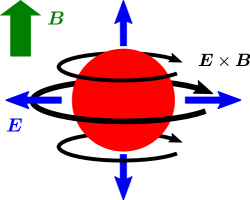
Figure 1: A charged object placed in a uniform magnetic field is surrounded by the Poynting vector $\boldsymbol{E}\times\boldsymbol{B}$ which carries an electromagnetic angular momentum contained in the conserved canonical angular momentum.

Still, the physical interpretation is quite non-trivial, we must say. Literally speaking, $J_{z}^{\rm field}$ is a purely electromagnetic contribution, and nevertheless, $\boldsymbol{E}$ extends from the charge source and in this sense we may well say that $\boldsymbol{E}$ is rather attributed to the matter property. If we are interested in the mechanical rotation as is the case in the Barnett and the Einstein–de Haas effects, however, we should count the kinetic angular momentum. Even in that case, this extra electromagnetic contribution could affect the kinetic angular momentum through the angular momentum conservation law.

5 Feynman’s angular momentum paradox and possible relevance to the relativistic nucleus-nucleus collision

Careful readers might have realized that the argument about $J_{z}^{\rm field}$ is essentially rooted in Feynman’s angular momentum paradox in classical physics. The paradox is articulated in The Feynman Lectures and the original setup is composed from a conductor disk with a solenoid that controls the magnetic strength. For detailed analysis of the original version of Feynman’s angular momentum paradox, see Ref. Fparadox for example. Here, let us discuss a simplified version of Feynman’s angular momentum paradox.

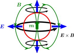
Figure 2: A charged thin sphere (red circle) and a magnetic moment at the center of the sphere. The dipolar magnetic fields and the Coulomb electric fields make circulating Poynting vectors.

We suppose that a thin sphere is uniformly charged (whose total amount is denoted by $Q$) and a finite magnetic moment $\boldsymbol{m}$ is fixed at the center of the sphere (see Fig. 2). The electric (outside of the sphere) and the magnetic profiles are, respectively,

$$\boldsymbol{E}=\frac{Q}{4\pi}\frac{\boldsymbol{x}}{r^{3}}\,,\qquad\boldsymbol{B}=\frac{1}{4\pi r^{3}}\biggl{(}\frac{3\boldsymbol{m}\cdot\boldsymbol{x}\boldsymbol{x}}{r^{2}}-\boldsymbol{m}\biggr{)}\,.$$ (38)

If $\boldsymbol{m}$ changes as a function of time, the magnetic field changes as well, which also results in an induction electric field due to Ampère’s law. Then, the charged sphere feels a moment of force under this induced electric field, $\boldsymbol{E}_{\rm ind}$, and the sphere is accelerated for rotation. The space integrated moment of force is, after some patient calculations, found to take a form of

$$\boldsymbol{N}=\int d\boldsymbol{S}\cdot\frac{\boldsymbol{x}\times Q\boldsymbol{E}_{\rm ind}}{4\pi R^{2}}=-\frac{Q\dot{\boldsymbol{m}}}{6\pi R}\,,$$ (39)

where $R$ denotes the radius of the sphere. Therefore, if $\boldsymbol{m}$ decreases, the sphere takes a positive moment of force to acquire a mechanical angular momentum. The question is; how can the angular momentum conservation law be satisfied? This phenomenon may sound similar to the Einstein–de Haas effect, but one should recall two important differences. One is that the object should be charge neutral in the Einstein–de Haas effect, and another is that in this classical example there is no magnetization at all. There are many variants of Feynman’s paradox, and they usually belong to classical physics (no spin effects).

Readers should be already aware of the resolution. As indicated in Fig. 2, the electromagnetic field generates circulating Poynting vectors. Actually, from explicit expressions of Eq. (38), we can obtain the angular momentum distribution as

$$\boldsymbol{x}\times(\boldsymbol{E}\times\boldsymbol{B})=\frac{Q}{(4\pi)^{2}r^{6}}(r^{2}\boldsymbol{m}-\boldsymbol{x}\boldsymbol{x}\cdot\boldsymbol{m})\,.$$ (40)

Therefore, the total angular momentum integrated in space outside of the sphere turns out to be,

$$\boldsymbol{J}^{\rm field}=\frac{Q\boldsymbol{m}}{6\pi R}\,.$$ (41)

It is obvious that the angular momentum in mechanical rotation originates from the loss in $\boldsymbol{J}^{\rm field}$, so that the total angular momentum is surely conserved. See Ref. doi:10.1119/1.15597 for related discussions on the Poynting vector contributions in classical electromagnetism. Interestingly this result of Eq. (41) was extended to the one-loop QED level which turned out to be free from a short-distance cutoff DAMSKI2019114828 .

In this classical example of Feynman’s paradox the essential point is that either $\boldsymbol{E}$ or $\boldsymbol{B}$ changes to make a finite difference in $\boldsymbol{x}\times(\boldsymbol{E}\times\boldsymbol{B})$ from which the mechanical rotation is induced. The novelty in the quantum mechanical example seen in the previous section is that quantum oscillations exhibit time dependence even for constant $\boldsymbol{E}$ and $\boldsymbol{B}$. In both cases the important lesson is that, as long as we prefer to use the Belinfante improved form for the EMT and the angular momenta, the covariant derivative in the matter sector makes all the expressions manifestly gauge invariant, and then we can access the kinetic angular momentum of the matter which is not necessarily conserved.

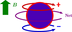
Figure 3: A net induced angular momentum with faster rotating positively and negatively charged particles. There are more positively charged particles in a plasma because of protons in the participant particles.

So far, we have been having general discussions not specifying any experimental realizations at all. Let us now consider some possible applications to the high-energy nucleus-nucleus collisions. It is known that the OAM in the non-central nucleus-nucleus collision can reach a gigantic value as large as $\sim 10^{5}\hbar$ as evaluated in the AMPT model Jiang:2016woz , supported by experimental data STAR:2017ckg . Here, we can make an order of magnitude estimate of extra angular momentum from the decay of the magnetic field using Eq. (37). Our following discussions may look different from Ref. Guo:2019mgh which addresses a possibility of the spin polarization by the induced electric fields. There are some discrepancies from spatial inhomogeneity as well as temporally decaying magnetic properties and also from hydrodynamic treatments, but we note that microscopically underlying physics is common.

The magnetic field created right after the collision is of order $eB\sim\text{GeV}^{2}$ at largest, and $\langle\rho^{2}\rangle$ in the collision geometry is around $\sim 10\,\text{fm}^{2}$. Therefore, if the magnetic field quickly decays whose time scale is $\sim 0.1\,\text{fm/c}$, this field angular momentum, $J_{z}^{\rm field}\sim 10\,\text{GeV}^{2}\!\cdot\!\text{fm}^{2}\sim 100\hbar$, is transferred to the angular momentum of single particle. The net charge is $0.1Z\sim Z$ depending on the impact parameter and the baryon stopping, where $Z\sim 100$ is the atomic number of the heavy nucleus, and so the net angular momentum is of order $10^{3}\sim 10^{4}\hbar$. Here, we would emphasize that the time scale is irrelevant. This angular momentum arises as a consequence of the conservation law and it is just there for any fast decaying $B$ (except loss by polarized photon emissions). From this simple estimate we can conclude that the net induced angular momentum is significantly smaller than the primarily produced angular momentum $\sim 10^{5}\hbar$. This is, however, not yet the end of the story. In reality of the nucleus-nucleus collision a plasma state consists of positively and negatively charged particles and the net charge is only its small fraction. Then, we can anticipate at least an order of magnitude larger angular momenta for positively and negatively charged components in the opposite directions which mostly cancel to lead to the net angular momentum (see Fig. 3). If this two-component model is a good approximation (which is dictated by the interaction strength between two components), each charged sector could carry the induced angular momentum $\sim 10^{4}\sim 10^{5}\hbar$, comparable to the primarily produced angular momentum. Interestingly, such a two-component picture with opposite rotation has been confirmed in the numerical simulation for the Einstein–de Haas effect in cold atomic systems PhysRevLett.96.080405 ; ebling2017einsteinde .

We have some more ideas [say, the global polarization should be also associated with the field angular momentum by Eq. (41) whose effect has never been studied] and have in mind applications to the local polarization measurements, but we shall stop our stories here. Such ideas as well as more detailed and quantitative calculations will be reported in a separate publication.

6 Epilogue

The interplay between the OAM and SAM is an old subject, but its entanglement with chirality in a relativistic framework is a quite new research field. The ultra-relativistic nucleus-nucleus collision experiments have been offering inspiring data and high-energy nuclear physicists have become wiser and wiser over decades. Some people, especially researchers close to but not directly in our field, might have assumed that physics of the relativistic nucleus-nucleus collision passed a peak. We must say, such an assumption is nothing but a hasty conclusion. The nucleus-nucleus collision still continues to provide us with surprises one after another.

Recent investigations on the OAM and SAM decomposition and their interactions are motivated by the $\Lambda$ and $\bar{\Lambda}$ polarization measurements, but we should emphasize that this is not a hip excitement. Theoretically speaking, this is an extremely profound subject, and there are still many things that nobody has understood. One common criticism against such kind of theory problem would be; what you call “profound” is just what I would call “academic”, or give me any measurable observable? Indeed it is not easy to make a new proposal for the nucleus-nucleus collision. Nevertheless, we can export our ideas inspired by the nucleus-nucleus collision to other physics fields such as cold atomic systems and laser optics. Still, even if exported ideas are adapted in a different shape, we can proudly say that this is a tremendous achievement from the high-energy nuclear physics!

We also emphasize that the OAM/SAM decomposition and also the EMT measurements are of central interest of the future coming electron-ion collider (EIC) physics. At least three pretty independent communities, the heavy-ion collision, the proton spin, and the laser optics have worked on the very similar physics, and now is the time to put all our wisdoms together toward the next generation breakthrough.

We would like to make acknowledgments. We thank Zebin Qiu for successful collaborations. K.F. is grateful to Kazuya Mameda for extremely useful discussions about ongoing projects on the Einstein–de Haas effect. K.F. also thanks Yoshi Hatta for interesting and critical (as always) conversations. K.F. also would like to acknowledge very useful and sometimes confusing (and so interesting) conversations with Francesco Becattini, Wojciech Florkowski, and Xu-Guang Huang.

References

- (1) K. Fukushima, S. Pu, and Z. Qiu, “Eddy magnetization from the chiral Barnett effect,” Phys. Rev. A99 (2019) 032105, arXiv:1808.08016 [hep-ph].
- (2) S. J. Barnett, “Gyromagnetic and electron-inertia effects,” Rev. Mod. Phys. 7 (1935) 129–166.
- (3) S. M. Barnett, “Relativistic electron vortices,” Phys. Rev. Lett. 118 (2017) 114802.
- (4) S. Tomonaga and T. Oka, The Story of Spin. University of Chicago Press, 1998.
- (5) E. Leader and C. Lorcé, “The angular momentum controversy: What’s it all about and does it matter?,” Phys. Rept. 541 (2014) 163–248, arXiv:1309.4235 [hep-ph].
- (6) M. Wakamatsu, “Is gauge-invariant complete decomposition of the nucleon spin possible?,” Int. J. Mod. Phys. A29 (2014) 1430012, arXiv:1402.4193 [hep-ph].
- (7) W. Florkowski, R. Ryblewski, and A. Kumar, “Relativistic hydrodynamics for spin-polarized fluids,” Prog. Part. Nucl. Phys. 108 (2019) 103709, arXiv:1811.04409 [nucl-th].
- (8) K. Hattori, M. Hongo, X.-G. Huang, M. Matsuo, and H. Taya, “Fate of spin polarization in a relativistic fluid: An entropy-current analysis,” Phys. Lett. B795 (2019) 100–106, arXiv:1901.06615 [hep-th].
- (9) F. Becattini and L. Tinti, “Thermodynamical inequivalence of quantum stress-energy and spin tensors,” Phys. Rev. D84 (2011) 025013, arXiv:1101.5251 [hep-th].
- (10) F. Becattini and L. Tinti, “Nonequilibrium thermodynamical inequivalence of quantum stress-energy and spin tensors,” Phys. Rev. D87 (2013) no. 2, 025029, arXiv:1209.6212 [hep-th].
- (11) F. Becattini, W. Florkowski, and E. Speranza, “Spin tensor and its role in non-equilibrium thermodynamics,” Phys. Lett. B789 (2019) 419–425, arXiv:1807.10994 [hep-th].
- (12) M. V. Berry, “Optical currents,” Journal of Optics A: Pure and Applied Optics 11 (2009) 094001.
- (13) X.-S. Chen, X.-F. Lu, W.-M. Sun, F. Wang, and T. Goldman, “Spin and orbital angular momentum in gauge theories: Nucleon spin structure and multipole radiation revisited,” Phys. Rev. Lett. 100 (2008) 232002, arXiv:0806.3166 [hep-ph].
- (14) R. P. Cameron, S. M. Barnett, and A. M. Yao, “Optical helicity, optical spin and related quantities in electromagnetic theory,” New Journal of Physics 14 (2012) 053050.
- (15) M. Wakamatsu, “On gauge-invariant decomposition of nucleon spin,” Phys. Rev. D81 (2010) 114010, arXiv:1004.0268 [hep-ph].
- (16) E. Leader, “The photon angular momentum controversy: Resolution of a conflict between laser optics and particle physics,” Phys. Lett. B756 (2016) 303–308, arXiv:1510.03293 [hep-ph].
- (17) Y. Hatta, “Gluon polarization in the nucleon demystified,” Phys. Rev. D84 (2011) 041701, arXiv:1101.5989 [hep-ph].
- (18) C. Lorcé, “Wilson lines and orbital angular momentum,” Phys. Lett. B719 (2013) 185–190, arXiv:1210.2581 [hep-ph].
- (19) M. Wakamatsu, Y. Kitadono, and P.-M. Zhang, “The issue of gauge choice in the Landau problem and the physics of canonical and mechanical orbital angular momenta,” Annals Phys. 392 (2018) 287–322, arXiv:1709.09766 [hep-ph].
- (20) C. R. Greenshields, R. L. Stamps, S. Franke-Arnold, and S. M. Barnett, “Is the angular momentum of an electron conserved in a uniform magnetic field?,” Phys. Rev. Lett. 113 (2014) 240404.
- (21) G. Lombardi, “Feynman’s disk paradox,” American Journal of Physics 51 (1983) 213–214.
- (22) J. Higbie, “Angular momentum in the field of an electron,” American Journal of Physics 56 (1988) 378–379.
- (23) B. Damski, “Electromagnetic angular momentum of the electron: One-loop studies,” Nucl. Phys. B949 (2019) 114828.
- (24) Y. Jiang, Z.-W. Lin, and J. Liao, “Rotating quark-gluon plasma in relativistic heavy ion collisions,” Phys. Rev. C94 (2016) 044910, arXiv:1602.06580 [hep-ph]. [Erratum: Phys. Rev.C95,no.4,049904(2017)].
- (25) STAR Collaboration, L. Adamczyk et al., “Global hyperon polarization in nuclear collisions: evidence for the most vortical fluid,” Nature 548 (2017) 62–65, arXiv:1701.06657 [nucl-ex].
- (26) X. Guo, J. Liao, and E. Wang, “Magnetic field in the charged subatomic swirl,” arXiv:1904.04704 [hep-ph].
- (27) Y. Kawaguchi, H. Saito, and M. Ueda, “Einstein–de Haas effect in dipolar Bose-Einstein condensates,” Phys. Rev. Lett. 96 (2006) 080405.
- (28) U. Ebling and M. Ueda, “Einstein-de Haas effect in a dipolar Fermi gas,” arXiv:1701.05446 [cond-mat.quant-gas].