First image then video: A two-stage network for spatiotemporal video denoising

Abstract

Video denoising is to remove noise from noise-corrupted data, thus recovering true signals via spatiotemporal processing. Existing approaches for spatiotemporal video denoising tend to suffer from motion blur artifacts, that is, the boundary of a moving object tends to appear blurry especially when the object undergoes a fast motion, causing optical flow calculation to break down. In this paper, we address this challenge by designing a first-image-then-video two-stage denoising neural network, consisting of an image denoising module for spatially reducing intra-frame noise followed by a regular spatiotemporal video denoising module. The intuition is simple yet powerful and effective: the first stage of image denoising effectively reduces the noise level and, therefore, allows the second stage of spatiotemporal denoising for better modeling and learning everywhere, including along the moving object boundaries. This two-stage network, when trained in an end-to-end fashion, yields the state-of-the-art performances on the video denoising benchmark Vimeo90K dataset in terms of both denoising quality and computation. It also enables an unsupervised approach that achieves comparable performance to existing supervised approaches.

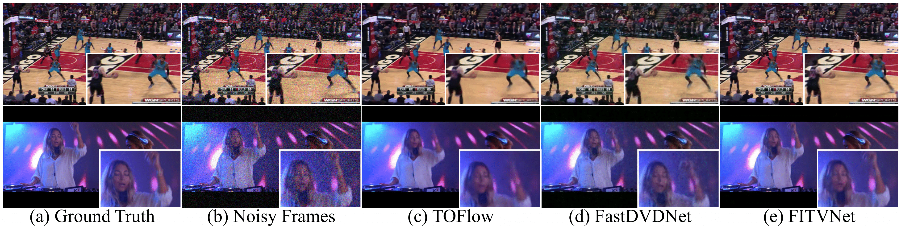
Figure 1: Samples of denoised frames of TOFlow, FastDVDNet, and our FITVNet model. In these cases, where an object undergoes a fast motion, TOFlow (c) fails to estimate motion accurately enough for effective denoising and noise-reduced frames appear blurry along object boundaries. Although FastDVDNet (d) avoids optical flow calculation, they still could not output better results as in since their spatiotemporal denoising block could hardly handle with both spatial noise and temporal deformation. In contrast, our FITV model (e) shows high performance even on these objects with a prior image denoising module for spatially reducing intra-frame noise.

1 Introduction

Image denoising is an important task to recover clean signal $I$ from noisy signal $\hat{I}=I+N$, where $N$ is some kind of noise added pixel by pixel. As an active research area for a long time, traditional methods [5] [14] have been proposed and achieved state-of-the-art results on many benchmarks. To further deal with real-world images without ground truth, unsupervised methods utilizing CNNs [2][13][16] [34] attempt to denoise only with noisy images and successfully train networks to approximate target data distribution. Although these methods always pose more assumptions and requirements on their inputs, they have achieved quite success.

As a more difficult task with the addition of temporal information, video denoising aims to recover clean signals $V=\{{I}_{1},{I}_{2},\dots,{I}_{T}\}$ from a noisy video $\hat{V}=V+\widetilde{N}$, where $\widetilde{N}=\{{N}_{1},{N}_{2},\dots,{N}_{T}\}$ and $\{{N}_{t}\}_{t=1}^{T}$ is the noise of each frame. In addition, video denoising can gain an advantage by proper modeling of inter-frame temporal deformation exists due to object motion in videos. For example, state-of-the-art TOFlow [36] approach tries to perform motion analysis and video denoising simultaneously in an end-to-end trainable network. However, we often observe blurry object boundaries in their denoised results when these objects undergo a fast motion as shown in Figure 1 (c) or when the foreground and background between these boundaries are of weak contrast due to say the low light environment. The blurry phenomenon happens because motion estimation breaks down for these objects in videos even in such a well-designed task-oriented flow estimation method.

Furthermore, the success application of convolutional neural networks (CNNs) to image denoising encourages researchers to design suitable neural models for video denoising. Although only invoking image denoising algorithm for each frame is not effective, the spatiotemporal denoising like V-BM4D[17], which extends BM3D [5] by searching similar patches in both spatial and temporal dimensions, is instructive. FastDVDNet[30], one state-of-the-art video denoising algorithm, extends flow-based DVDNet [29] by employing modified U-Net [24] architectures to realize spatiotemporal denoising with the powerful representation of CNNs. This avoids explicit estimation of objection motion, but the results shown in Figure 1(d) demonstrate that the spatiotemporal denoising block still could not handle high-speed moving objects well because spatial noise distribution and temporal deformation are very different and dealing with them together in a mixed fashion is too challenging. The limited capability of spatiotemporal denoising block brings the main motivation of our work: Can we address this challenge by separating CNN-based spatiotemporal denoising into a two-stage procedure, in which the first module tries to spatially reduce the intra-frame noise in ${N}_{t}$ and the second module, still as regular spatiotemporal inter-frame video denoising, is able to handle these cases with the help of “processed” inputs of the first stage?

In order to formulate such a first-image-then-video (FITV) two-stage denoising process in an end-to-end network, we propose our neural model, called FITVNet. We realize the first module with an image-to-image network architecture, which reduces the noise within each single image/frame via spatial processing, and the second module as a regular spatiotemporal video denoising network. These two modules are jointly supervised by a proposed loss function with a balanced learning ratio between each other in different training phases. With such a training procedure, output features of the first stage show high denoising performance for reducing intra-frame noise, especially along object boundaries where TOFlow and FastDVD fail to recover. In addition to designing such an end-to-end network for video denoising, we empirically demonstrate the effectiveness of such a two-stage denoising method via extensive comparison with state-of-the-art video denoising approaches in terms of both denoising quality and computation. We also introduce an unsupervised video denoising approach.

The main contributions of our work are as below.

• We propose a two-stage video denoising algorithm which reduces intra-frame noise spatially first and then applies spatiotemporal video denoising, which achieves high denoising performance everywhere including boundaries of fast-moving objects.

• We integrate these two stages in an end-to-end trainable network with one supervision signal for these two different modules. We also explore incorporating different types of supervision signals.

• We achieve state-of-the-art video denoising results on the benchmarking Vimeo90K dataset in terms of both denoising quality and computation. Our completely unsupervised video denoising approach achieves comparable performance to current supervised approaches.

Figure 2: The FTIV denoising framework of our model. Its simple idea of adding a single-image based denoising module before regular video denoising is proven effective.

2 Previous Works

2.1 Image denoising

Image denoising has been explored for a long time and recent methods  [3] [14] [18] [27]  [33] [37] [15]  [31] make use of the representative capability of CNNs rather than traditional methods [5] [25] [28]. These methods take pairs of noisy and clean images as inputs to train their models. Then models could learn a mapping function from noisy image distribution ${P}_{Y}={P}_{X}+{P}_{noise}$ to real image distribution ${P}_{X}$ via minimizing a loss function between their outputs and corresponding clean images, and achieve better results than traditional state-of-the-art models such as BM3D [5].

But clean images are expensive to obtain when facing with real-world scenarios. To tackle such a difficulty, Noise2Noise [16] utilizes the relationship between the ${P}_{Y}$ and ${P}_{X}$ distributions and trains its model using pairs of both noisy images of the same scene. Following the similar vein, Noise2Void [13] Noise2Self [2], and Noise-As-Clean [34] have recently been proposed, which alleviates the hard requirement used in Noise2Noise that pair images should be with the same scene and independently sampled with the same noise distribution. In this work, we will incorporate the idea of Noise2Noise into the FITVNet.

2.2 Video denoising

Although image denoising has attracted so much research interest, video denoising is still under-explored. Directly applying image denoising algorithm to each video frame fails to capture the temporal relationship between consecutive frames. To handle with the key problem of motion estimation in video denoising, traditional methods [23] [35] are used for flow calculation in video denoising. Later works [7] [10] [22] propose end-to-end networks for flow estimation. Then TOFlow [36] and DVDNet [29] further simultaneously predict optical flows and denoise frames instead of separating these two tasks as in [20], and obtain state-of-the-art results that are better than V-BM4D [17], which is similar to VNLB [1] as extensions of BM3D [5]. However, image warping between neighbouring frames using the estimated flow field is time consuming. Even worse, the flow calculation tends to be inaccurate when an object undergoes fast motion or when the image contrast between the foreground and background is weak, leading to the over-smoothness and loss of details along object boundaries in the denoised frames. Alternatively, ViDeNN [4] and FastDVDNet [30] propose one end-to-end network to realize spatiotemporal denoising as [9]  [19] [32] have done in video inpainting. Both of them feed pairs of noisy and clean videos to networks to successively reduce noise in input frames. Similarly, NLNet [6] fuses a CNN with a self-similarity search strategy in video denoising and VINet [11] successfully applies CNNs in video inpainting. Furthermore, [8] proposes a blind denoising approach based on DnCNN [37] and Noise2Noise, which motivates us to utilize unsupervised image denoising algorithm in video denoising process. In this work, we will go beyond one spatiotemporal video denoising network and propose a two-stage FITVNet for both supervised and unsupervised video noising.

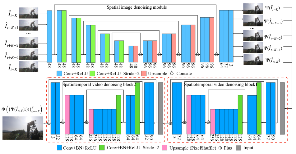
Figure 3: The whole flow chart of our model. In the first stage, we remove intra-frame noise spatially via image denoising module. Then we apply spatiotemporal denoising module in the second stage to remove the rest of noise via spatiotemporal processing.

3 Method

To describe our model clearly, we first formulate the theoretical background of FITVNet in this section. Then we show details about these two denoising stages, including network architectures, loss function employed for these two parts, different variants of our FITVNet, etc. Figure 2 visualizes the diagram of FITVNet.

3.1 Theoretical background

As mentioned before, object motion is an essential information between neighbouring frames in video denoising and optical flow is always employed to estimate the motion. Consider $2K$ neighbouring frames ${I}_{t-K}(x),{I}_{t-K+1}(x),\dots,{I}_{t+K-1}(x),{I}_{t+K}(x)$ around the reference frame ${I}_{t}(x)$ in a clean video, the relationship between each neighbouring frame and the reference frame is formulated as follows, assuming “constancy of brightness”:

$${I}_{t+k}(x)={I}_{t}(x+{\delta}_{k}x);\quad k\in\{-K,\dots,K-1,K\},$$ (1)

where ${\delta}_{k}x$ denotes the estimated optical flow field between these two frames. When the optical flow field is of small magnitude, we use the first-order Taylor approximation so that temporal deformation becomes “additive”:

$${I}_{t+k}(x)\approx{I}_{t}(x)+J_{t}(x){\delta}_{k}x,$$ (2)

where $J_{t}(x)$ is the Jacobian matrix. In real-world, we observe noisy frames:

$$\begin{split}{\hat{I}}_{t+k}(x)&={I}_{t+k}(x)+{N}_{k}(x)\\ &={I}_{t}(x+{\delta}_{k}x)+{N}_{k}(x)\\ &\approx{I}_{t}(x)+J_{t}(x){\delta}_{k}x+{N}_{k}(x),\ \end{split}$$ (3)

where ${N}_{k}(x)$ is noise added for each frame, such as additive white Gaussian noise (AWGN).

What DVDNet [29] achieves in this theoretical framework is to learn an approximate mapping function $T$. It essentially incorporates two functions: the first is to estimate optical flow ${\delta}_{k}x$ between observed neighbouring frames and reference frame, and the second is to utilize these intermediate variables to predict clean reference frame ${I}_{t}$, which can be represented in the following formula:

$${I}_{t}(x)=T\left(\{{\hat{I}}_{t+k}(x-{\delta}_{k}x)\}_{k=-K}^{K}\right).$$ (4)

While both functions are implemented using two isolated networks, TOFlow [36] takes a further step that achieves simultaneous estimation of optical flow and fusion of warped frames via end-to-end learning, thus obtaining state-of-the-art performance. However, Figure 1 shows that precise flow estimation, even for TOFlow, is hard.

An alternative method, such as FastDVDNet, applies spatiotemporal denoising, skipping these sub-optimal flow calculation. It performs the following formula:

$${I}_{t}(x)=\Phi\left(\{{\hat{I}}_{t+k}(x)\}_{t=-K}^{K}\right),$$ (5)

where $\Phi$ performs spatiotemporal processing and is approximated by CNNs. However, the failure in denoising fast-moving objects with apparent, blurry object boundaries, motivates us to sort the spatiotemporal denoising into two-stage denoising process as introduced before. More formally, what our FITVNet really does is to remove noise in ${\hat{I}}_{t+k}$ in advance via a function $\Psi$, followed by $\Phi$ :

$$\begin{split}{I}_{t}(x)=\Phi\left(\{\Psi({\hat{I}}_{t+k}(x))\}_{t=-K}^{K}\right).\end{split}$$ (6)

With our prior image denoising results as inputs, denoted by $\{\Psi({\hat{I}}_{t+k}(x))\}_{t=-K}^{K}$, regular spatiotemporal denoising function $\Phi$ deals with “cleaner” frames, which makes the task less challenging.

3.2 The spatial image denoising stage

For the first image denoising stage, we use a modified architecture of Noise2Noise [16] to approximate the above mapping function $\Psi$, which tries to spatially remove intra-frame noise in an input sequence of $2K+1=5$ frames. The module is composed of $2K+1$ networks that share the same architectures and parameters as shown in Figure 3. Each network, which processes its corresponding frame, is trained with the following ${l}_{2}$ loss function:

$${\cal L}_{pd}=\Sigma_{k=-K}^{K}\|{\Psi}_{\theta}({\hat{I}}_{t+k})-{I}_{t+k}\|_{2},$$ (7)

where $\{{\hat{I}}_{t+k}\}_{k=-K}^{K}$ are input frames, $\{{\Psi}_{\theta}\}_{k=-K}^{K}$ are mapping functions of the corresponding frames, ${\theta}$ is network parameters of this module, and $\{{I}_{t+k}\}_{k=-K}^{K}$ denote the target supervision signal of input frames.

Especially for the network architecture of this module, we replace original pooling layers with convolutional layers with a stride of two in order to capture more contexts. This helps reduce noise level, especially for boundaries of moving objects so that the following spatiotemporal module learns better everywhere with these pre-denoised frames.

To test the performance of our model with different target signals, we have implemented the following three models with different loss functions ${\cal L}_{pd}$:

• FITVNet (base): without supervision signal of ${L}_{pd}$ introduced before;

• FITVNet (+jsn): with noisy frames as the target signal in ${\cal L}_{pd}$ just like what Noise2Noise [16] has done and ${\cal L}_{pd}$ becomes:

  $${\cal L}_{pd}=\Sigma_{k=-K}^{K}\|{\Psi}_{\theta}({\hat{I}}_{t+k})-{\tilde{I}}_{t+k}\|_{2},$$ (8)

  where ${\tilde{I}}_{t+k}$ is noisy frames with Gaussian noise i.i.d to the noise of ${\hat{I}}_{t+k}$; and

• FITVNet (+jsc): with clean frames as the target signal in ${\cal L}_{pd}$.

Note that other unsupervised image denoising methods such as Noise2Void [13] Noise2Self [2], and Noise-As-Clean [34] can also be used, which we will explore in future.

Furthermore, the success of FITVNet (+jsn), which trains our first module in an unsupervised manner, unleashes the potential of our model to a completely unsupervised video denoising scenario as discussed in Section 3.4.

3.3 The spatiotemporal video denoising stage

In spatiotemporal video denoising stage, we use another network to capture temporal information between neighbouring frames, that is, it takes more frames as inputs to utilize object motion information among these frames. Concretely, the module takes $2K+1$ consecutive prior denoised frames $\{\Psi({\hat{I}}_{t-K}),\dots,\Psi({\hat{I}}_{t+K-1}),\Psi({\hat{I}}_{t+K})\}$, among which the central one is chosen as the reference frame to be denoised, as inputs and clean frame ${I}_{t}$ as ground truth. Meanwhile, the ${l}_{2}$ loss is used to supervise the learning process of the module as in (9):

$${\cal L}_{st}=\Sigma_{i}\|{\Phi}_{\gamma}\left(\{{\Psi}_{\theta}({\hat{I}}_{t+k}(x))\}_{k=-K}^{K}\right)-{I}_{t}\|_{2},$$ (9)

where ${\Phi}_{\gamma}$ is the mapping function of regular video denoising block, and ${I}_{t}$ denotes the clean reference frame. However, the output features of pre-denoising module would influence performance of the current spatiotemporal denoising module, so we add a decay coefficient $\alpha$ to balance ${\cal L}_{pd}$ with ${\cal L}_{st}$ in the jointly supervised manner, and the final loss function for our model is as follows:

$$\frac{\alpha}{e}{\cal L}_{pd}+{\cal L}_{st}.$$ (10)

where $e$ denotes the total number of epochs before this iteration.

Unlike flow-based methods, such as PWC-Net [26] and TOFlow [36], such CNN-based spatiotemporal denoising network needs to model spatial noise and temporal deformation within one module. We realize this module via the method employed in FastDVDNet [30], which uses one block to process every three consecutive frames in the totally five frames and then feed concatenated output features of the first block to the other block as shown in Figure 3. This avoids explicit flow calculation which is sub-optimal in these flow-based models and the experiments show that the representative capability of CNNs help avoid boundary blurry appearing in TOFlow with the help of prior image denoising. Furthermore, the expensive computation of warping operations in flow-based methods is also eliminated.

3.4 Unsupervised FITVNet

With the success of applying prior image denoising stage before regular video denoising stage and training the module with noisy images as in FITVNet (+jsn), we have the opportunity to design a completely unsupervised approach for video denoising. Here we modify (9) by replacing ${I}_{t}$ with ${\Psi}_{\theta}({\hat{I}}_{t})$ as follows:

$${\cal L}_{st}=\Sigma_{i}\|{\Phi}_{\gamma}\left(\{{\Psi}_{\theta}({\hat{I}}_{t+k}(x))\}_{k=-K}^{K}\right)-{\Psi}_{\theta}({\hat{I}}_{t})\|_{2}.$$ (11)

This avoids the use of ground truth as clean signal.

Meanwhile, during training we enlarge the decay coefficient $\alpha$ to ensure that there is enough iterations for the first stage to learn to map a better ${\Psi}_{\theta}({\hat{I}}_{t})$, which would provide cleaner signal for the second stage.

4 Experimental Results

Method	Vimeo-Gauss25		Vimeo-Mixed
	PSNR	SSIM	PSNR	SSIM
TOFlow	33.14	0.9119	33.40	0.9126
FITVNet (base)	33.17	0.89	32.62	0.88
FITVNet (+jsc)	34.33	0.9208	33.93	0.9168

Table 1: Quantitative results. Compared with TOFlow, our FITVNet (+jsc) model achieves consistently better results.

We utilize the large-scale, high-quality Vimeo90K dataset, which is built along with TOFlow [36], for benchmarking our video denoising model, It consists of 89,800 videos of size 256x448, which covers various real-world scenes and actions. We randomly choose 700 videos from whole test dataset, denoted as Vimeo700, for the following testing experiments as the original test dataset is too large.

4.1 Setup

In all experiments, we use two kinds of noises: AWGN of $\sigma\in[5,80]$ and mixed noise of Gaussian noise with standard deviation of 25.5 and 10% salt-and-pepper noise (Vimeo-Mixed), to train models for comparison with previous methods, including flow-based networks and end-to-end training networks. We also train two models. The first is trained with the Vimeo-Mixed noise for a fair comparison with TOFlow [36] and for demonstrating that our model is capable to deal with such kind of noise. The other is trained with the AWGN noise for a fair comparison with FastDVDNet [30] and for demonstrating the superiority of our proposed prior image denoising stage.

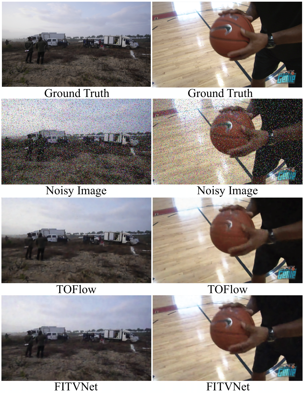
Figure 4: The denoised results of our model and TOFlow on Vimeo700 with mixed noise. Details are over-smooth in the TOFlow results while our model could recover these more clearly.

In our experiments, we randomly choose $2K+1$ frames from the original video if the total number of frames of that video exceeds $2K+1$. We do not employ any pretraining procedure used in TOFlow[36]. We use the commonly used metrics of Peak Signal-to-Noise Ratio (PSNR) and Structural SIMilariry index (SSIM) to characterize our denoising performance.

The whole network with two models is implemented in PyTorch [21] with a mini-batch of size 16. We optimize the final loss function $\alpha{\cal L}_{sd}+{\cal L}_{st}$ via ADAM [12] optimizer with default hyperparameters. In addition, the total number of epochs is by default set to 40 (unless further explained) and the learning rate is set to be 0.0001.

4.2 Comparison with flow-based network

In the following, we compare our model with TOFlow, which is a state-of-the-art flow-based video denoising network. Table 1 quantitatively reports experimental results, which demonstrate the capability of our model to deal with mixed noise in addition to commonly used Gaussian noise. The model has been trained on Vimeo-Mixed for 40 epochs with hyperparameters mentioned before. Compared with TOFlow, our FITVNet (base) model achieves comparable performance in terms of both PSNR and SSIM and our FITVNet (+jsc) model achieves consistently better results.

Also our two-stage video denoising method alleviates the over-smooth phenomenon happened in TOFlow as we can observe in Figure 4. For example, in the left column of Figure 4, clothes that these two people wear are green, which are similar to the background around them, and the denoised results by TOFlow could not recover such details in this area. Similar phenomenon has also happened even worse in the right column of results, where the basketball holder moves fast, and the logo of that basketball is too obscure in the denoised video of TOFlow. In contrast, such details are obviously clearer in our results.

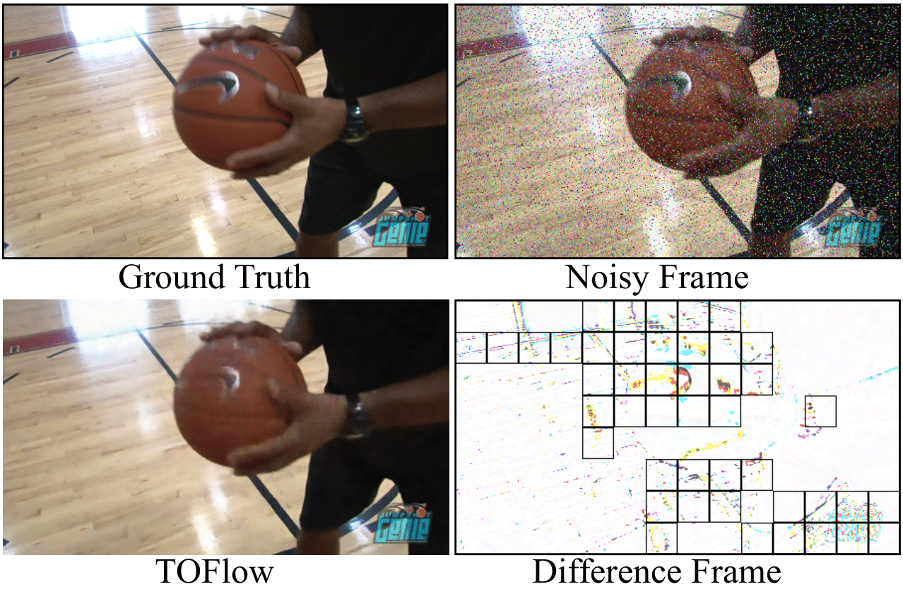
Figure 5: Here we show the difference image between a denoised frame of TOFlow and its corresponding clean frame and use black boxes to bound patches whose std is higher than the average std 0.0222. Resulted bounding boxes successfully bound the boundaries of the person, basketball, and the logo on the basketball.

Method	${AD}_{avg}$	${AD}_{max}$	#$AD$
TOFlow	0.0263	0.0617	304
FITVNet (+jsc)	0.0260	0.0585	298

Table 2: Quantitative characterization of over-smooth phenomenon. Compared with TOFlow, our FITVNet (+jsc) model is slightly advantageous.

Method	Time (s)
TOFlow	0.2460
FITVNet (+jsc)	0.0466

Table 3: Comparison of running time to denoise an RGB frame of resolution 256x448. Compared with TOFlow, our FITVNet (+jsc) model is more than 5 times faster.

Method	Vimeo-Gauss15		Vimeo-Gauss25		Vimeo-Gauss35		Vimeo-Gauss45		Vimeo-Gauss55
	PSNR	SSIM	PSNR	SSIM	PSNR	SSIM	PSNR	SSIM	PSNR	SSIM
TOFlow	31.64	0.8719	33.14	0.9195	32.70	0.8849	30.70	0.8352	28.59	0.7732
FastDVDNet	33.85	0.9114	32.13	0.8754	30.77	0.8387	29.63	0.7990	28.70	0.7589
FITVNet (base)	30.73	0.8664	35.21	0.9248	33.78	0.9118	32.64	0.8935	31.73	0.8760
FITVNet (+jsn)	36.76	0.9475	34.80	0.9270	33.41	0.9078	32.34	0.8896	31.44	0.8723
FITVNet (+jsc)	37.70	0.9552	35.45	0.9326	33.89	0.9118	32.68	0.8926	31.72	0.8744
FITVNet (unsupervised)	34.23	0.8944	32.79	0.8743	31.72	0.8557	30.83	0.8377	30.02	0.8202

Table 4: Quantitative results. Compared with TOFlow and FastDVDNet, our baseline FITVNet model is consistently better except that our base model fails with the ’Gauss15’ setting, while our other FITVNet models are robust when supervised with ${\cal L}_{pd}$.

To quantitatively characterize such a problem existing in TOFlow, we propose to compute Average Deviation (AD). Based on the difference image ${I}_{diff}$ between each predicted image $\hat{I}$ and the corresponding clean image $I$, we first divide the image ${I}_{diff}$ into $K$ nonoverlapping patches of size $32*32$ and calculate the standard deviation $\rho(k)$ for each patch $k$. Then, we select those patches whose $\rho(k)$ is larger than a threshold $\bar{\rho}$ we set as the average of $\{\rho(k);k=1:K\}$, denoted by $\bar{\rho}$. Finally, we compute the average of the selected $\rho(k)$ as the AD index.

$$AD=\frac{\sum_{k:\rho(k)>{\bar{\rho}}}\rho(k)}{\sum_{k:\rho(k)>{\bar{\rho}}}1}.$$ (12)

When the over-smooth phenomenon happens along the boundaries of fast-moving objects, the difference image has structural residuals, which contribute to high values of $\rho(k)$, such that the phenomenon are likely captured by the proposed AD index. In Figure 5, we also visually show this. Specifically, we use black boxes to bound those selected patches, Obviously, we successfully localize the boundaries of the fast moving objects such as basketball, logo and the person, which coincides with our visual perception.

In experiments, we compute the average of $AD$ (${AD}_{avg}$) and the max of $AD$ (${AD}_{max}$) of all test images on Vimeo700. We also tally the total number of test images (#$AD$) whose $AD$ is larger than ${AD}_{avg}$. The above three statistics are shown in Table 2. Although ${AD}_{avg}$ is similar for these two models, TOFlow yields higher values of ${AD}_{avg}$, ${AD}_{max}$ and #$AD$, which indicates that TOFlow likely suffers from the over-smoothing problem than FITVNet. This concides with Figure 4 too.

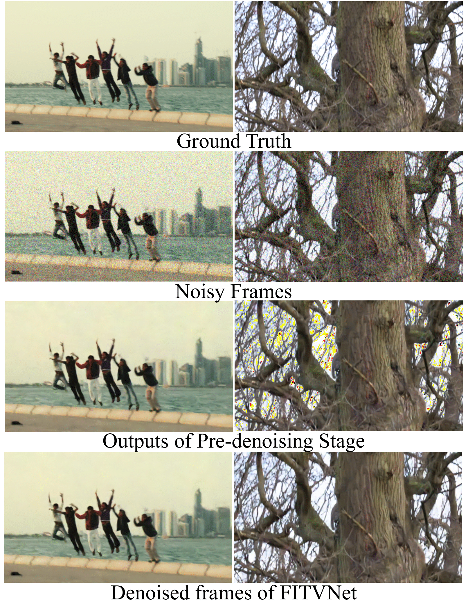
Figure 6: Output images of the prior image denoising module and the final denoised frames. The output images are clear, and spatial noise is largely reduced, fostering the following video denoising module to learn better results.

Running time. TOFlow improves traditional flow-based networks to utilize a convolutional network to predict optical flow of neighbouring frames. However, the warping operation also takes more computation in the whole process. In contrast, our FITVNet method achieves fast inference with the help of direct network implementation. As shown in Table 3, it takes only 46.6ms to denoise a 256x448 RGB frame, while TOFlow needs 246ms. The experiments are all run on the same GPU of NVIDIA 2080ti card.

4.3 Comparison with end-to-end methods

Then we compare our model with FastDVDnet [30], which is a spatiotemporal video denoising algorithm, based on Vimeo700 with AWGN of different levels. The models are all trained on Vimeo90K, and results are shown in Table 4. It is obvious that our three variants perform much better than FastDVDNet, even though our base model is only supervised with ${\cal L}_{st}$. Besides, we also test TOFlow on Vimeo700 with Gaussian noise with the TOFlow’s open checkpoint model since we have no access to TOFlow’s training process. The TOFlow results are robust, but not as good as the performance on Vimeo-Mixed. Although our FITVNet (base) model performs not very well with ‘Gauss15’, the other two variants, FITVNet (+jsc) and FITVNet (+jsn), are stable across all noise levels with the help of the ${\cal L}_{pd}$ loss.

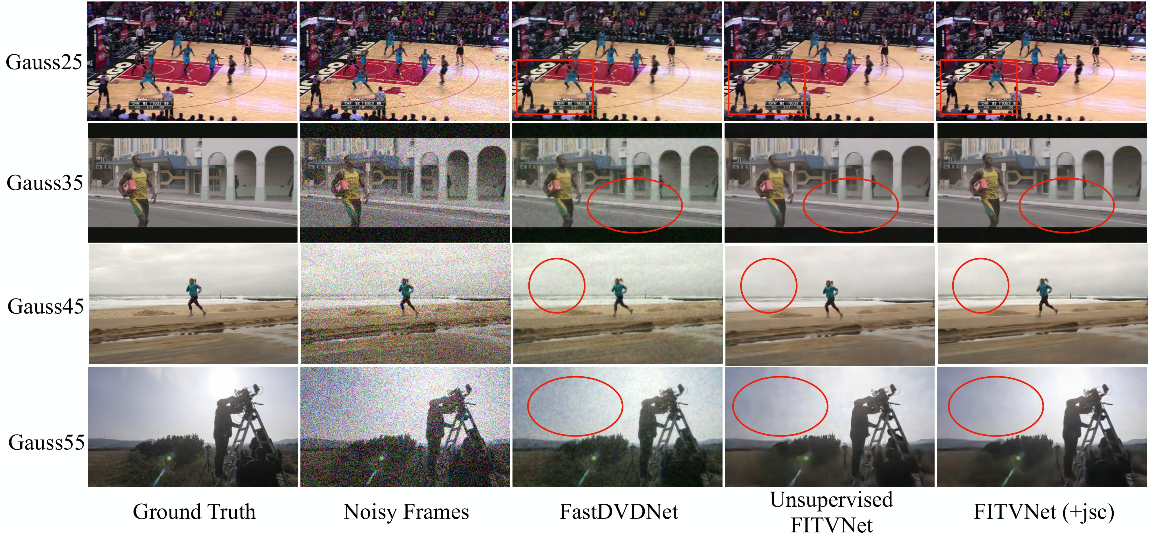
Figure 7: We qualitatively show the results of FastDVDNet, our best model FITVNet (+jsc), and our unsupervised FITVNet. FITVNet (+jsc) performs the best on all these cases, no matter with fast-moving objects or with highly noisy backgrounds. Besides, unsupervised FITVNet performs comparablely with FastDVDNet. FastDVDNet could recover more details while unsupervised FITVNet is capable of removing more spatial noise with help of prior image denoising module.

To further demonstrate the effect of prior image denoising module, we visualize the outputs of this module in Figure 6. From the left subfigure, we could observe that the output image is already clean so that the following spatiotemporal module would just learn to model object motion this time. On the other hand, in the case shown in the right subfigure, the prior image denoising module does not remove all spatial noise, and the following spatiotemporal module would learn to model both spatial noise and temporal deformation this time. These two cases characterize how the first and the second modules cooperate with each other to accomplish video denoising tasks with state-of-the-art results.

Furthermore, we qualitatively show in Figure 7 the denoised frames of our models and the FastDVDNet at different noise levels. It can be easily perceived that the FITVNet results are visually more pleasing than the FastDVDNet results. For the background regions where we bound with red boxes and circles, our results evidently possess higher visual quality. Furthermore, along the boundaries of moving objects as in the ‘Gauss25’ setting, the results appear sharper.

4.4 Unsupervised experiment

We also test our unsupervised FITVNet as introduced in Section 3.4 and the results are also shown in Table 4. Although its performance is not as good as FITVNet with clean frames as supervision, it achieves better performance than FastDVDNet across the board in terms of PSNR and comparable performance to TOFlow on Vimeo700. Note that both FastDVDNet and TOFlow are supervised with clean frames. The running time of unsupervised FITVNet is the same as that of other FITVNet models.

Besides, we also qualitatively show our denoised frames in Figure 7. It is evident that our denoised frames exhibit less spatial noise when compared with FastDVDNet, which emphasizes the importance of prior image denoising module. The success of our completely unsupervised denoising model also demonstrates the power of our simple yet effective idea for such a two-stage video denoising framework.

5 Conclusion

In this work, we propose a two-stage approach called FITVNet for video denoising task, which first reduces the noise frame by frame and then applies spatiotemporal denoising. This aims to address the challenge that the boundaries of fast moving objects in the denoised results obtained by previous models, which either estimate object motion via optical flow or directly apply spatiotemporal denoising, tend to be blurry. In addition, our model is supervised and is learned in an end-to-end manner; but it also renders the possibility of a purely unsupervised learning approach. Our extensive evaluations based on the Vimeo90K dataset demonstrate that the proposed FITVNet recovers object boundaries more clearly and achieve state-of-the-art denoising results in terms of quantitative measures such as PSNR and SSIM while running over 5 times faster than TOFlow. Furthermore, the purely unsupervised FITVNet, implemented by replacing supervision signal of the second module with the output of the first module, achieves comparable denoising performance to FastDVDNet.

The failure of our base model with the ‘Gauss15’ setting in Table 4 suggests that implicit object motion estimation with a direct spatiotemporal networks is not as stable as flow-based model. In future, we plan to explore the possibility of integrating flow calculation into our FITVNet for improved robustness and performance. We also plan to explore more along unsupervised video denoising.

6 Appendix

To make the experimental setup more clearly, we would display detailed network architectures of two modules in FITVNet. In the meanwhile, we would exhibit more denoised examples.

Name	${N}_{out}$	Description
Input	12	Three frames with noise map
Enc_Conv1a	3x30	Convolution 3x3
Enc_Conv1b	32	Convolution 3x3
Enc_Conv1c	64	Convolution 3x3 Stride 2
Enc_Conv2a	64	Convolution 3x3
Enc_Conv2b	64	Convolution 3x3
Enc_Conv2c	128	Convolution 3x3 Stride 2
Enc_Conv3a	128	Convolution 3x3
Enc_Conv3b	128	Convolution 3x3
Dec_Conv3a	128	Convolution 3x3
Dec_Conv3b	128	Convolution 3x3
Dec_Conv3c	256	Convolution 3x3
Dec_Upsample3	64	PixelShuffle
Dec_Plus3	64	Plus Output of Enc_Conv2b
Dec_Conv2a	64	Convolution 3x3
Dec_Conv2b	64	Convolution 3x3
Dec_Conv2c	128	Convolution 3x3
Dec_Upsample2	32	PixelShuffle
Dec_Plus2	32	Plus Output of Enc_Conv1b
Dec_Conv1a	32	Convolution 3x3
Dec_Conv1b	3	Convolution 3x3
Dec_Plus1	3	Plus Reference frame

Table 5: Network Architecture of spatiotemporal video denoising module.

6.1 Network Architectures

The proposed FITVNet consists of three modified U-Net [24], of which one is used for the spatial image denoising module and presented in Table 6, while the other two are for spatiotemporal video denoising module and displayed in Table 5. Note that ${N}_{out}$ denotes the number of output channels and each convolution layer is followed by a ReLU activation layer (unless further explained).

6.2 Comparison with TOFlow and FastDVDNet via Sobel operator

In Section 4.2, We have showed the performance of object boundaries recovery of FITVNet, TOFlow [36], and FastDVDNet [30] with our proposed AD index. Next, we further exhibit processed results with Sobel operator in Figure 6.2. The operator is a traditional boundary detection method, which gives the direction of the largest possible increase from light to dark and the rate of change in that direction according to calculations of the gradient of the image intensity at each point.

As results shown in Figure 6.2, FastDVDNet is the worst one since Sobel is not noise sensitive, i.e., the denoised results of FastDVDNet are still with a higher noise level. Although TOFlow and FITVNet both show high performance on denoising these videos, FITVNet deals with object boundaries of fast-moving objects, i.e. the woman in the shown video, better than TOFlow.

Ground Truth

FITVNet

FastDVDNet [30]

TOFlow [36]

Name	${N}_{out}$	Discription
input	3	One frame
Enc_Conv0	48	Convolution 3x3
Enc_Conv1a	48	Convolution 3x3
Enc_Conv1b	48	Convolution 3x3 Stride 2
Enc_Conv2a	48	Convolution 3x3
Enc_Conv2b	48	Convolution 3x3
Enc_Conv3a	48	Convolution 3x3 Stride 2
Enc_Conv3b	48	Convolution 3x3
Enc_Conv4a	48	Convolution 3x3
Enc_Conv4b	48	Convolution 3x3 Stride 2
Enc_Conv5a	48	Convolution 3x3
Enc_Conv5b	48	Convolution 3x3
Enc_Conv6	48	Convolution 3x3 Stride 2
Dec_Upsample5	48	Upsample 2x2
Dec_Concat5	96	Concatenate Output of Enc_Conv4b
Dec_Conv5a	96	Convolution 3x3
Dec_Conv5b	96	Convolution 3x3
Dec_Upsample4	96	Upsample 2x2
Dec_Concat4	144	Concatenate Output of Enc_Conv3b
Dec_Conv4a	96	Convolution 3x3
Dec_Conv4b	96	Convolution 3x3
Dec_Upsample3	96	Upsample 2x2
Dec_Concat3	144	Concatenate Output of Enc_Conv2b
Dec_Conv3a	96	Convolution 3x3
Dec_Conv3b	96	Convolution 3x3
Dec_Upsample2	96	Upsample 2x2
Dec_Concat2	144	Concatenate Output of Enc_Conv1b
Dec_Conv2a	96	Convolution 3x3
Dec_Conv2b	96	Convolution 3x3
Dec_Upsample1	96	Upsample 2x2
Dec_Concat1	96+3	Concatenate Input
Dec_Conv11	64	Convolution 3x3
Dec_Conv11	32	Convolution 3x3
Dec_Conv0	3	Convolution 3x3 LeakyReLU($\alpha$=0.1)

Table 6: Network Architecture of spatial image denoising module.

References

- [1] Pablo Arias and Jean-Michel Morel. Video denoising via empirical bayesian estimation of space-time patches. Journal of Mathematical Imaging and Vision, 60(1):70–93, 2018.
- [2] Joshua Batson and Loic Royer. Noise2self: Blind denoising by self-supervision. arXiv preprint arXiv:1901.11365, 2019.
- [3] Harold C Burger, Christian J Schuler, and Stefan Harmeling. Image denoising: Can plain neural networks compete with bm3d? In 2012 IEEE conference on computer vision and pattern recognition, pages 2392–2399. IEEE, 2012.
- [4] Michele Claus and Jan van Gemert. Videnn: Deep blind video denoising. pages 0–0, 2019.
- [5] Kostadin Dabov, Alessandro Foi, Vladimir Katkovnik, and Karen Egiazarian. Image denoising by sparse 3-d transform-domain collaborative filtering. IEEE Transactions on image processing, 16(8):2080–2095, 2007.
- [6] Axel Davy, Thibaud Ehret, Gabriele Facciolo, Jean-Michel Morel, and Pablo Arias. Non-local video denoising by cnn. arXiv preprint arXiv:1811.12758, 2018.
- [7] Alexey Dosovitskiy, Philipp Fischer, Eddy Ilg, Philip Hausser, Caner Hazirbas, Vladimir Golkov, Patrick Van Der Smagt, Daniel Cremers, and Thomas Brox. Flownet: Learning optical flow with convolutional networks. In Proceedings of the IEEE international conference on computer vision, pages 2758–2766, 2015.
- [8] Thibaud Ehret, Axel Davy, Jean-Michel Morel, Gabriele Facciolo, and Pablo Arias. Model-blind video denoising via frame-to-frame training. In Proceedings of the IEEE Conference on Computer Vision and Pattern Recognition, pages 11369–11378, 2019.
- [9] Jia-Bin Huang, Sing Bing Kang, Narendra Ahuja, and Johannes Kopf. Temporally coherent completion of dynamic video. ACM Transactions on Graphics (TOG), 35(6):196, 2016.
- [10] J Yu Jason, Adam W Harley, and Konstantinos G Derpanis. Back to basics: Unsupervised learning of optical flow via brightness constancy and motion smoothness. In European Conference on Computer Vision, pages 3–10. Springer, 2016.
- [11] Dahun Kim, Sanghyun Woo, Joon-Young Lee, and In So Kweon. Deep video inpainting. In Proceedings of the IEEE Conference on Computer Vision and Pattern Recognition, pages 5792–5801, 2019.
- [12] Diederik P Kingma and Jimmy Ba. Adam: A method for stochastic optimization. arXiv preprint arXiv:1412.6980, 2014.
- [13] Alexander Krull, Tim-Oliver Buchholz, and Florian Jug. Noise2void-learning denoising from single noisy images. In Proceedings of the IEEE Conference on Computer Vision and Pattern Recognition, pages 2129–2137, 2019.
- [14] Stamatios Lefkimmiatis. Non-local color image denoising with convolutional neural networks. In Proceedings of the IEEE Conference on Computer Vision and Pattern Recognition, pages 3587–3596, 2017.
- [15] Stamatios Lefkimmiatis. Universal denoising networks: a novel cnn architecture for image denoising. In Proceedings of the IEEE conference on computer vision and pattern recognition, pages 3204–3213, 2018.
- [16] Jaakko Lehtinen, Jacob Munkberg, Jon Hasselgren, Samuli Laine, Tero Karras, Miika Aittala, and Timo Aila. Noise2noise: Learning image restoration without clean data. arXiv preprint arXiv:1803.04189, 2018.
- [17] Matteo Maggioni, Giacomo Boracchi, Alessandro Foi, and Karen Egiazarian. Video denoising, deblocking, and enhancement through separable 4-d nonlocal spatiotemporal transforms. IEEE Transactions on image processing, 21(9):3952–3966, 2012.
- [18] Xiao-Jiao Mao, Chunhua Shen, and Yu-Bin Yang. Image restoration using convolutional auto-encoders with symmetric skip connections. arXiv preprint arXiv:1606.08921, 2016.
- [19] Alasdair Newson, Andrés Almansa, Matthieu Fradet, Yann Gousseau, and Patrick Pérez. Video inpainting of complex scenes. SIAM Journal on Imaging Sciences, 7(4):1993–2019, 2014.
- [20] Simon Niklaus and Feng Liu. Context-aware synthesis for video frame interpolation. In Proceedings of the IEEE Conference on Computer Vision and Pattern Recognition, pages 1701–1710, 2018.
- [21] Adam Paszke, Sam Gross, Soumith Chintala, Gregory Chanan, Edward Yang, Zachary DeVito, Zeming Lin, Alban Desmaison, Luca Antiga, and Adam Lerer. Automatic differentiation in pytorch. 2017.
- [22] Anurag Ranjan and Michael J Black. Optical flow estimation using a spatial pyramid network. In Proceedings of the IEEE Conference on Computer Vision and Pattern Recognition, pages 4161–4170, 2017.
- [23] Jerome Revaud, Philippe Weinzaepfel, Zaid Harchaoui, and Cordelia Schmid. Epicflow: Edge-preserving interpolation of correspondences for optical flow. In Proceedings of the IEEE conference on computer vision and pattern recognition, pages 1164–1172, 2015.
- [24] Olaf Ronneberger, Philipp Fischer, and Thomas Brox. U-net: Convolutional networks for biomedical image segmentation. In International Conference on Medical image computing and computer-assisted intervention, pages 234–241. Springer, 2015.
- [25] Stefan Roth and Michael J Black. Fields of experts: A framework for learning image priors. In 2005 IEEE Computer Society Conference on Computer Vision and Pattern Recognition (CVPR’05), volume 2, pages 860–867. Citeseer, 2005.
- [26] Deqing Sun, Xiaodong Yang, Ming-Yu Liu, and Jan Kautz. Pwc-net: Cnns for optical flow using pyramid, warping, and cost volume. In Proceedings of the IEEE Conference on Computer Vision and Pattern Recognition, pages 8934–8943, 2018.
- [27] Ying Tai, Jian Yang, Xiaoming Liu, and Chunyan Xu. Memnet: A persistent memory network for image restoration. In Proceedings of the IEEE international conference on computer vision, pages 4539–4547, 2017.
- [28] Marshall F Tappen, Ce Liu, Edward H Adelson, and William T Freeman. Learning gaussian conditional random fields for low-level vision. In 2007 IEEE Conference on Computer Vision and Pattern Recognition, pages 1–8. IEEE, 2007.
- [29] Matias Tassano, Julie Delon, and Thomas Veit. Dvdnet: A fast network for deep video denoising. 2019.
- [30] Matias Tassano, Julie Delon, and Thomas Veit. Fastdvdnet: Towards real-time video denoising without explicit motion estimation. arXiv preprint arXiv:1907.01361, 2019.
- [31] Martin Weigert, Loic Royer, Florian Jug, and Gene Myers. Isotropic reconstruction of 3d fluorescence microscopy images using convolutional neural networks. In International Conference on Medical Image Computing and Computer-Assisted Intervention, pages 126–134. Springer, 2017.
- [32] Yonatan Wexler, Eli Shechtman, and Michal Irani. Space-time video completion. In Proceedings of the 2004 IEEE Computer Society Conference on Computer Vision and Pattern Recognition, 2004. CVPR 2004., volume 1, pages I–I. IEEE, 2004.
- [33] Junyuan Xie, Linli Xu, and Enhong Chen. Image denoising and inpainting with deep neural networks. In Advances in neural information processing systems, pages 341–349, 2012.
- [34] Jun Xu, Yuan Huang, Li Liu, Fan Zhu, Xingsong Hou, and Ling Shao. Noisy-as-clean: Learning unsupervised denoising from the corrupted image. arXiv preprint arXiv:1906.06878, 2019.
- [35] Jia Xu, René Ranftl, and Vladlen Koltun. Accurate optical flow via direct cost volume processing. In Proceedings of the IEEE Conference on Computer Vision and Pattern Recognition, pages 1289–1297, 2017.
- [36] Tianfan Xue, Baian Chen, Jiajun Wu, Donglai Wei, and William T Freeman. Video enhancement with task-oriented flow. International Journal of Computer Vision, 127(8):1106–1125, 2019.
- [37] Kai Zhang, Wangmeng Zuo, Yunjin Chen, Deyu Meng, and Lei Zhang. Beyond a gaussian denoiser: Residual learning of deep cnn for image denoising. IEEE Transactions on Image Processing, 26(7):3142–3155, 2017.