Complexity and Efficient Algorithms for Data Inconsistency Evaluating and Repairing
Abstract
Data inconsistency evaluating and repairing are major concerns in data quality management. As the basic computing task, optimal subset repair is not only applied for cost estimation during the progress of database repairing, but also directly used to derive the evaluation of database inconsistency. Computing an optimal subset repair is to find a minimum tuple set from an inconsistent database whose remove results in a consistent subset left. Tight bound on the complexity and efficient algorithms are still unknown. In this paper, we improve the existing complexity and algorithmic results, together with a fast estimation on the size of optimal subset repair. We first strengthen the dichotomy for optimal subset repair computation problem, we show that it is not only APXcomplete, but also NPhard to approximate an optimal subset repair with a factor better than for most cases. We second show a -approximation whenever given functional dependencies, and a -approximation when an -portion of tuples have the -quasi-Turn property for some . We finally show a sublinear estimator on the size of optimal S-repair for subset queries, it outputs an estimation of a ratio with a high probability, thus deriving an estimation of FD-inconsistency degree of a ratio . To support a variety of subset queries for FD-inconsistency evaluation, we unify them as the -oracle which can answer membership-query, and return tuples uniformly sampled whenever given a number . Experiments are conducted on range queries as an implementation of -oracle, and results show the efficiency of our FD-inconsistency degree estimator.
1 Introduction
A database instance is said to be inconsistent if it violates some given integrity constraints, that is, contains conflicts or inconsistencies. Those database inconsistencies can occur in various scenarios due to many causes. For example, a typical scenario is information integration, where data are integrated from different sources, some of them may be low-quality or imprecise, so that conflicts or inconsistencies arise.
In the principled approach managing inconsistencies [5], the notion of repair was first introduced decades ago. A repair of an inconsistent instance is a consistent instance obtained by performing a minimal set of operations on so as to satisfy all the given integrity constraints. Repairs could be defined under different settings of operations and integrity constraints. We follow the setting of [27], where we take functional dependencies, also a most typical one, as the integrity constraints, and deletions as the operations, so that a repair of here is a subset of obtained by minimal tuple deletions, and an optimal repair of is a subset of it obtained by deleting minimum tuples. Computing an optimal subset repair with respect to functional dependencies is the major concern in this paper. It is a fundamental problem of data inconsistency management and the motivation has been partially discussed in [27]. The significance of study on computing optimal repair is twofold.
Computing optimal repairs would be the basic task in data cleaning and repairing. For data repairing, existing methods could be roughly categorized into two classes, fully automatic and semi automatic ways [14]. In fully automatic repairing methods, optimal subset repairs are always considered as optimization objectives [15, 32, 31]. Given an inconsistent database, one needs automated methods to make it consistent, i.e., find a repair that satisfies the constraints and minimally differs from the originated input, optimal subset repair is right one of the choices [27]. On the other side, optimal subset repairs are also preferred candidates picked by automatic data cleaning or repairing system when dealing with inconsistency errors. Instead of the fully automatic way, the human-in-loop semi-automatic repairing is another prevailing way [6, 7, 18, 22], and the complement of an optimal subset repair is an ideal lower bound of repairing cost which could be used as to estimate the amount of necessary effort to eliminate all the inconsistency, sometimes even enlighten them how to choose specific operations.
Besides optimal repairs, measuring inconsistency motivates the computation on the size of optimal repairs. Intuitively, for the same schema and with the same integrity constraints, given two databases instances, it is natural to know which one is more inconsistent than the other. This comparison can be accomplished by assigning a measure of inconsistency to a database. Hence, measuring database inconsistency has been revisited and generalized recently by data management community. [9] argued that both the admissible repair actions and how close we want stay to the instance at hand should be taken into account when defining such measure. To achieve this, database repairs [8] could be applied to define degrees of inconsistency. Among a series of numerical measurements proposed in [9], subset repair based inconsistency degree is the most typical one. According to [9], subset repair based inconsistency degree is defined as the ratio of minimum number of tuple deleted in order to remove all inconsistencies, i.e., the size of the complement of an optimal subset repair. Therefore, computing optimal subset repair is right the fundamental of inconsistency degree computation. Previous studies does not provide fine-grained complexity on this problem and efficient algorithm for large databases. Thus, we in this paper give a careful analysis on the computational complexity and fast computation on the size of an optimal subset repair. Contributions of this paper are detailed as follows.
We first study the data complexity of optimal subset repair problem including the lower and upper bounds in order to understand how hard the problem is and how good we could achieve. The most recent work [27] develops a simplification algorithm and establishes a dichotomy based on it to figure the complexity of this problem. Simply speaking, they show that, for the space of combinations of database schemas and functional dependency sets, (i) it is polynomial to compute an optimal subset repair, if the given FD set can be simplified into an empty set; (ii) the problem is APX-complete, otherwise.
As the computation accuracy of the size of an optimal subset is very crucial to our motivation, we strengthen the dichotomy in this paper by improving the lower bound into concrete constants. Specifically, we show that it is NPhard to obtain a -optimal subset repair for most input cases, and –optimal subset repair for all the others. We show that a simple reduction could unify most cases and improve the low bound We then consider approximate repairing. For this long standing problem, it is always treated as a vertex cover problem equivalently, and admits the upper bound of ratio . However, we take a step further, show that (i) an -approximation of an optimal subset repair could be obtained for given functional dependencies, more than that, (ii) it is also polynomial to find an -approximation, which is much better if an -portion of tuples have the -quasi-Turn property for some .
Then, we turn to the most related problem, to estimate the subset repair based FD-inconsistency degree efficiently. For an integrated database instance, it is helpful to measure the inconsistency degree of any part of it locally, in order to let users know and understand well the quality of their data. Consider an inconsistent database integrated by data from two organizations and , we need to know the main cause of the conflicts. If we know the inconsistency degree of some part is very low but that of is as high as the inconsistency degree of , then we could conclude that the cause of inconsistencies is mainly on the conflicts in between, but not in any single source. That is when we find the inconsistency degree of some local part is approximately equal to that of the global one, then it is reasonable to take this part as a primary cause of inconsistency, so that we may focus on investigating what happens in .
To this motivation, in this paper, we focus on fast estimating the subset-repair based FD-inconsistency degree. We here follow the definition of subset repair based measurement recently proposed by Bertossi [9], and develop an efficient method estimating FD-inconsistency degree of any part of the input database. Concretely, it seems a same problem as computing an optimal repair itself, so that the complexity result of optimal subset repair computing indicates it is hard to be approximated within a better ratio polynomially, not to mention linear or even a sublinear running time. However, we observe that, the value of inconsistency degree is a ratio to the size of input data, say , hence, an -fold accuracy loss of optimal subset repair size estimating is acceptable. Therefore, we develop a sample-based method to estimate the size of an optimal subset repair with a error of so as to break through the limitation of linear time complexity while achieving an approximation with an additive error . To support a variety of subset queries, especially for whose result is very large, we model those queries as the -oracle which can answer membership-query, and return tuples uniformly sampled whenever given a number .
The following parts of this paper is organized as follows. Necessary notations and definitions are formally stated in Section 2. Complexity results and LP-based approximations are shown in Section 3. Sampling-based fast FD-inconsistency degree estimation is given in Section 4. Experiment results are discussed in Section 5. At last, we conclude our study in Section 6.

2 Problem Statement
The necessary definitions, notations and problem definition are formally given in this section.
Schemas and Tables.
A -ary relation schema is represented by , where is the relation name and are distinct attributes of .
In the following part of this paper, we refer to for simplicity. We customarily use capital letters from the beginning of the English alphabet to denote individual attribute, such as “”, and use capital letters from the end of the English alphabet individual attribute to denote a set of attributes, such as “”, sometimes with subscripts.
A set of attributes are conventionally written without curly braces and commas, such as can be written as if .
We assume the domain of each attribute, , is countably infinite,
then, any instance over relation is a collection of -ary tuples ,
where each value are taken from the set .
Let refer to the value on attribute , and refer to the sequence of attribute values when .
We use to denote the set of all tuples from sharing the same value of .
The size of an instance is the number of tuples in it, denoted as .
In this paper, any instance of a relation schema is a single table corresponding to .
Functional Dependencies. Let and be two arbitrary sets of attributes in a relation schema , then is said to be functionally determined by , written as , if and only if each -value in is associated with precisely one -value in . Usually is called the determinant set and the dependent set, but in this paper, for the sake of simple, we just call them determinant and dependent respectively. A functional dependency is called trivial if is a subset of .
Given a functional dependency over , any instance corresponding to is said to satisfy , denoted as , such that for any two tuples in , if . That is, two tuples sharing the same values of will necessarily have the same values of . Otherwise, does not satisfy , denoted as . As a special case, any two-tuple subset of is called a -conflict in with respect to if .
Let be a set of functional dependencies, we usually use to refer to the number of functional dependencies in , i.e. . Given a set of functional dependency , an instance is said to be consistent with respect to if satisfies every functional dependencies in . Otherwise, is inconsistent, denoted as . As a special case, any two-tuple subset of is called a conflict in if there is some such that is a -conflict. That is, contains one or more conflicts if is inconsistent.
Example 1.
Our running example is around the schema order(id, name, AC, PR, PN, STR, CTY, CT, ST, zip). Each tuple contains information about an item sold (a unique item id, name and price PR), and the phone number (area code AC, phone number PN) and the address of the customer who purchased the item (street STR, country CTY, city CT, state ST). An instance of the schema order is shown in figure 1(a). Some functional dependencies on the order database include:
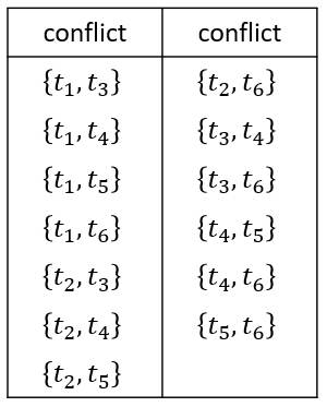
The database of figure 1(a) is inconsistent since there are 13 -conflicts in total as listed in figure 1(b). The meaning of the number assigned to each conflict will be clarified later.
Equivalence Class. Given an FD : , an instance can be partitioned horizontally into several determinant equivalence classes according to the -values, that is, tuples in each determinant equivalence class share the same value of . Moreover, any determinant equivalence class can be further partitioned into several determinant-dependent equivalence classes according to the -values, denoted as , that is, tuples in each determinant equivalence class share the same value of . It is obviously that, for an FD and any instance , two tuples and not in any -conflict in must be in different determinant equivalence classes and respectively.
Example 2.
With respect to , instance can be partitioned into one determinant equivalence class and 4 determinant-dependent equivalence classes , , and .
Repair. Let be an instance over a relation schema , a subset of is an instance obtained from by eliminating some tuples. If is a subset of , then the distance from to , denoted , is the number of tuples missing from , and it is for sure that , thus,
Let be an instance over schema , and let be a set of FDs. A consistent subset of with respect to is a subset of such that . A subset repair (s-repair, for short) is a consistent subset that is not strictly contained in any other consistent subset. An optimal subset repair of is a consistent subset of such that is minimum among all consistent subsets of . Note that, each optimal subset repair is a repair, but not necessarily vice versa. Clearly, any consistent subset can be polynomially transformed into a subset repair, with no increase of distance. Unless explicitly stated otherwise, in this paper, we do not distinguish between a subset repair and a consistent subset.
Example 3.
Both and are s-repairs of . It is easy to verify that is an optimal s-repair such that .
Now, we formally define the first problem studies in this paper as follows,
Definition 1 (OSR Computing).
Input an instance over a relation schema , a functional dependency set , OSR computing problem is to compute an optimal s-repair of with respect to .
Inconsistency Measurement. Computing an optimal s-repair helps estimating database FD-inconsistency degree. As in literature [9], given a functional dependency set , one of subset repair based measurements on the FD-inconsistency degree of input database is defined as following,
Moreover, this measurement could be also applied for any part of the input database in order to evaluate its corresponding FD-inconsistency degree as following,
The local degree does not depends on the whole of the input data, thus leads to the right equation. Our FD-inconsistency degree of any part is defined locally, hence, we use notation instead of by omitting the first parameter. Then, we here formally define the second problem studied in this paper as follows,
Definition 2 (FD-inconsistency Evaluation).
Input a relation schema , an FD set , an instance over and a subset query on , FD-inconsistency evaluation is to compute of the query result with respect to .
Example 4.
As mentioned in Example 3, is an optimal s-repair of , then . Given a range query on attribute PR in order, the result set . ia also an optimal s-repair of , then .
Approximation. We follow the convention of approximation definition, to define the approximation of optimal repairs explicitly. For a constant , a -optimal s-repair is an s-repair of such that
for all s-repairs of . In particular, an optimal s-repair is the same as a -optimal s-repair.
According to the definition of subset repair based FD-inconsistency degree, for an arbitrary and a constant , is a -approximation of such that
Complexity. The conventional measure of data complexity are adopted to perform the computational complexity analysis of optimal subset repair computing problem in this paper. That is, the relation schema and the functional dependency set are fixed in advance, and the instance data over is the only input. Therefore, an polynomial running time may have an exponential dependency on and . In such context of data complexity, each distinct setting of and indicates a distinct problem of finding an optimal repair, so that different setting may indicate different complexities. Recall that, in the measurement of combined complexity, the relation schema and the functional dependency set are considered as inputs, hence, the hardness of OSR computing problem equals to that of vertex cover problem. However, this is not the case under data complexity.
After showing the hardness, we still adopt data complexity to be the measurement on running times and approximation ratios, however, the difference is that we fix only the size of the functional dependency set , but not itself and the schema. Note that, this is reasonable in practical, the input functional dependencies may vary with time, but the number of given functional dependencies are always much smaller than the size of input data , so that we could consider it to be bounded within some constant.
3 Computing An Optimal S-Repair
In this section, we show the improved lower bound and upper bound of OSR.
3.1 The Strengthened Dichotomy for OSR
Livshits et al.gave a procedure OSRSucceed() [27] to simplify a given functional dependency set . Any functional dependency set can either be simplified polynomially into a set containing only trivial functional dependencies, or not. The procedure OSRSucceed() returns true for the former case, otherwise false. OSR is polynomially tractable for functional dependency sets that can be simplified into trivial ones. For all the other functional dependency sets, OSR computing problem is hard as in not only NPhard but also APXcomplete.
Specifically, any functional dependency set that cannot be simplified further can be classified into one of five certain classes of functional dependency sets. And OSR is shown in APXcomplete for any such functional dependency set by fact-wise reductions from one of the following four fixed schemas.
| = | ||
| = | ||
| = | ||
| = |
By showing the inapproximability of such four schemas, the following dichotomy follows immediately.
Theorem 1 (Dichotomy for OSR computing [27])
Let be a set of FDs, then
-
•
An optimal subset repair can be computed polynomially, if OSRSucceed() returns true;
-
•
Computing an optimal subset repair is APXcomplete, if OSRSucceed() returns false.
In this paper, we give a more careful analysis to show a concrete constant for each of the four schemas, thus strengthening this dichotomy.
Lemma 1
For FD sets , , and , there is no polynomial-time -approximation algorithm for computing an optimal subset repair for any , unless NP=P.
Proof.
We here show three similar gap-preserved reductions (i.e., ) from MAX NM-E3SAT to show the lower bound. Note that, (i) any variable do not occur more than once in any clause, and (ii) each clause is monotone as either (++) or (++). Each of the following reductions generates a corresponding table instance with schema .
MAX NM-E3SAT . For each clause , build three tuples. If contains a positive literal of variable , then build . If contains a negative literal of variable , then build . Intuitively, guarantees that exactly one of the three tuples survives once the corresponding clause is satisfied, and will ensure the consistent assignment of each variable.
MAX NM-E3SAT . By simply exchange the column B and C, we get the second reduction. Concretely, for each clause , build three tuples. If contains a positive literal of variable , then build . If contains a negative literal of variable , then build . Intuitively, guarantees that exactly one of the three tuples survives once the corresponding clause is satisfied, and will ensure the consistent assignment of each variable.
MAX NM-E3SAT . By slightly modify the way of tuple generation, we get the third reduction.
Concretely, (i) for each variable , build two -tuples and , (ii) for each clause , build three -tuples, if contains a positive literal of variable , then build ,if contains a negative literal of variable , then build .
Intuitively, there are tuples created, guarantees that exactly one of the three tuples survives once the corresponding clause is satisfied, and will ensure the consistent assignment of each variable.
Lower bound. We here show the proof for , and the other two are similar. For any instance of MAX NM-E3SAT problem, we denote the corresponding table built by reduction as . Let be the number of clauses satisfied by an assignment on , and be the number of clauses satisfied by an optimal assignment on .
Claim 1
Any tuple deletion should contain at least two of the three tuples having the same value on the attribute for any .
Claim 2
any tuple deletion should contain either the set of tuples or the set of tuples for any .
FD guarantees the first claim, and FD ensures that there is always an assignment can be derived from ,
Claim 3
Let be an minimum tuple deletion, then any optimal solution does not contain and simultaneously for each variable .
Proof by contradiction. Suppose if not, there must exist another solution obtained by returning tuple or from into without producing any inconsistency, thus resulting in a solution smaller than the optimal one. Based on the three claims, we have
and for any solution of ,
additionally, we have the fact that
Now, suppose is an -approximation () of such that , then
| (1) | |||||
since each clause has exactly 3 literals, we have
apply this fact in the right hand of inequality (1), it is
since , therefore we get
apply this into inequality (1), then
That is, if there is an -approximation of OSR, then MAX NM-E3SAT can be approximated within . However, if OSR can be polynomially approximated within , then there exists a polynomial approximation better than for MAX NM-E3SAT problem, but it contraries to the hardness result shown in [23].
One can verify the lower bound of and in the same way, then the lemma follows immediately. One can refer to appendix for more detail. ∎
To deal with the last case, by carefully merging the four -reductions MAX B29-3SAT 3DM [24] 3DM MAX 3SC [24] MAX 3SC Triangle [4] Triangle [27] , we have the following lemma.
Lemma 2
For FD set , there is no polynomial time -approximation algorithm for computing an optimal subset repair for any , unless NP=P.
Proof.
By merging the -reduction mentioned above, if computing an OSR for FD set can be approximated within , then there exists a polynomial approximation better than for MAX B29-3SAT problem which is contrary to the hardness result shown in [17]. ∎
Based on Lemma 1,2 and Theorem 1, a strengthened dichotomy for OSR computing can be stated as follows.
Theorem 2 (A strengthened dichotomy for OSR)
Let be a set of FDs, then
-
•
An optimal subset repair can be computed polynomially, if OSRSucceed() returns true;
-
•
There is no poly-time ()-approximation to compute an optimal subset repair, if OSRSucceed() returns false and can be classified into the class having a fact-wise reduction from to itself;
-
•
There is no poly-time ()-approximation to compute an optimal subset repair, otherwise.
For the polynomial-intractable side, one can simply verify that if the size of FD set is unbounded, then the OSR computing is as hard as classical vertex cover problem on general inputs which is NPhard to be approximate within for any . A simple approximation algorithm can provide a ratio of 2 when the input FD set is unbounded.
However, in practical, the size of FD set is usually much smaller than the size of data, so that it can be treated as fixed, especially in the context of big data. Unfortunately, it is still unclear how good we could arrive when the size of FD set is bounded. Therefore, to study the upper bound of its data complexity, we next give a carefully designed approximation to archive a ratio of when the number of given FDs is , or even better sometimes.
3.2 Approximation
To investigate the upper bound of optimal s-repair computing problem, we start from a basic linear programming to provide a ratio of , for an input instance over a given relation schema and an input FD set , where is the number of all possible determinant-dependent equivalence classes of an input instance with respect to the input FD set . Then, an improved the approximation ratio could be derived by means of triad elimination. Finally, we find another -approximation which is sometimes, but not always, better than , based on a -quasi-Turn characterization of the input inconsistent instance with respect to the input .
3.2.1 A basic approximation algorithm
We start from the basic linear programming model which is equivalent to the classical one solving minimum vertex cover problem.
Let be a 0-1 variable indicating the elimination of tuple such that, if eliminate ; otherwise. Then we formulate the OSR computing problem as followings,
| (2) | |||||
| (3) | |||||
| (4) |
It is well-known that every extreme point of this model takes value of 0 or 0.5 or 1, hence, we can relax it with condition:
thus getting
A trivial rounding derives a ratio of immediately. However, based on a partition of instance with respect to FD set , a better ratio depending on the size of partition could be obtained.
Obviously, for any FD of with a size of , each tuple belongs to one and only one distinct determinant-dependent equivalence class with respect to , say , then we have
where Hence, we observe that if any two tuples and are in some conflict, then there must be
and vice versa, since they disagree on at least one attribute in some but agree on all the attributes in .
Further more, another observation is that all the tuples in conflict with are included in the determinant equivalence classes
Because all tuples in each may be inconsistent with each other at worst, hence, every tuple in may be inconsistent with at most tuples.
Let be the numbers of tuples who are in conflict with , and be the numbers of consistent classes that could be partitioned into, such that each class is consistent. This observation implies the following claims immediately,
Claim 4
This claim implies that all the tuples in could be partitioned into at most classes such that tuples in each class are consistent with each other.
Then, we improve the ratio by using the partitions of the input instance. Based on the rounding technique similar with [29], an improved approximated algorithm could be stated as follows.
Input:
-tuple instance over schema , FD set
Output:
optimal subset repair of with respect to
Obviously, can be returned in polynomial time as shown in [33], and it is easy to see that is a s-repair. In fact, if an and not be picked into deletion , then all the tuples in conflicts with must be added into because they are not in partition , and the sum of two variables of tuples in any conflict should be no less than . Therefore, we claim that the approximation ratio is .
Lemma 3
Algorithm 1 returns a -optimal subset repair.
Proof.
Define notations , and as follows,
Then, the following holds obviously,
Second, We have that
Therefore, is a -optimal subset repair of . ∎
The number is unbounded, in the worst case, could be as large as so that it is a factor depending on the size of input.
3.2.2 Improved ratio by triad eliminating
Reducing the number of consistent partitions will improve the approximation. We introduce triad elimination in this section to decrease the partition number into a factor which is independent with the size of input but only depending on the number of input functional dependencies.
Data reduction. Let be three tuples in , then they are called a triad if any two of them are in a conflict with respect to . An important observation is that any s-repair contains at most one tuple of a triad in , especially in an optimal s-repair, hence, any triad elimination yields a -optimal s-repair of itself. Therefore, we could preform a data reduction by eliminating all the disjoint triads without the loss of an approximation ratio .
Based on the data reduction, the improved algorithm can be shown as follow.
Input:
-tuple instance over schema , FD set
Output:
optimal subset repair of with respect to
Let be the number of functional dependencies in , then we claim that TE LP-OSR will return a better approximation as the following theorem.
Theorem 3
Algorithm TE LP-OSR returns a -optimal subset repair.
Proof.
Algorithm 2 does find an s-repair, because all the triads are eliminated from , hence conflicts involving any tuples in are removed from , and all conflicts in the reduced data are removed by Baseline-LP-OSR.
Moreover, any optimal s-repair of contains at most one tuples of a triad which yields a -approximation for the subset of , formally, we have,
Additionally, consider each determinant equivalence class with respect to any single FD, no triad in it, that is, could be partitioned into 2 consistent classes with respect to this FD. It implies could be partitioned into consistent classes with respect to . Due to lemma 3, is a -optimal s-repair of .
Let be the optimal s-repair of , then,
And is an s-repair of , hence,
Without loss of generality, we have , then Algorithm 2 returns a -approximation. ∎
Remarks. Note that this ratio depends on only the size of functional dependency set other than the scale of input data. Therefore, a simple corollary implies a ratio of 1.5 for , , and , and 1.75 for , no matter how large of the input data.
A naive enumeration of triad is time wasting. In our algorithm, as in the proof of theorem 3, it is not necessary to eliminate all disjoint triads as possible. Instead, to obtain a good ratio, it needs only eliminate all disjoint triads with respect to each single functional dependency. Then, for each single functional dependency, sorting or hashing techniques could be utilized to speed up the triad eliminating, and skip the finding of triads across different functional dependencies.
3.2.3 Improved ratio by k-quasi-Turn property
Triad elimination based TE LP-OSR does not capture the characteristic of input data instance. We next give another approximation algorithm QT LP-OSR. In fact, we found that constraints could be derived to strengthen LP formula. Intuitively, for each functional dependency, each determinant equivalence class contains several determinant-dependent equivalence classes, say , hence, tuples in at least classes should be eliminated from to obtain an s-repair. Therefore, constraints could be invented to limit the lower bound of variables taking value according to the classes, so that a better ratio could be obtained for some featured cases.
Formally, consider a determinant equivalence class containing determinant-dependent equivalence classes , …, , hence,
-quasi-Turn. Given , a tuple is of -quasi-Turn property if and only if there is some functional dependency and a determinant equivalence class with respect to such that
Example 5.
As mentioned in Example 2, given the functional dependency , the determinant equivalence class is partitioned into determinant-dependent equivalence classes. It is easy to verify that is a -quasi-Turn
Then we characterize the data with parameter which is the portion of -quasi-Turn tuples in . A strengthened LP could be formulated as follows,
In this model, pick a small enough , the inequality guarantees that in any integral solution, at least variables taking value of . However, in the fractional solution, we could not limit the number of -variables, for example, a slop line cannot distinguish points , and . However, even so, we will show that this number could still be limited to improve the approximation ratio.
Claim 5
Every extreme point of any solution to the linear programming is in .
One can simply verify the correctness and prove it by contradiction, we omit the proof here.
Every solution of this strengthened linear programming still admits the half-integral property, hence, we take the basic rounding strategy such that
then, for tuples in each determinant equivalence class , at most variables will be rounded as wrongly. Formally, for each determinant equivalence class , define and as follows,
then we have the following lemma,
Lemma 4
,
Proof.
Due to the constraint
hence,
The worst case is that , then we have,
that is
Pick small such that , then this lemma follows. ∎
This lemma derives the a ratio depending on the portion of -quasi-Turn tuples where for any .
Theorem 4
QT LP-OSR returns a -optimal subset repair.
Proof.
Let be the fractional optimal solution of the strengthened LP, thus Consider the subset of all the -quasi-Turn tuples, let the solution intersecting with is . Let be the approximated s-repair, then in , the number of tuples rounded out of the approximated s-repair,
and
then we derive the ratio as follows
Then for the other part,
Therefore we have ∎
Combine the approximations based on the strengthened LP and the triad elimination, a better approximation is provided. Note that, it is polynomial-time to find a best pair to capture the data characteristic as possible, so as to improve the ratio as much as possible.
4 Fast Estimate FD-Inconsistency Degree
The hardness of OSR computing implies FD-inconsistency degree evaluation is also hard. Therefore, we take effort to find an approximation of such degree. Fortunately, an observation is that we aim to compute the ratio, but not any OSR itself, hence, to achieve a constant relative ratio, a relaxation of approximation ratio with an factor is allowed. In this section, we show a fast FD-inconsistency evaluation of subset query result. To obtain a good approximation in sublinear complexity, we allow a relative ratio and an additional additive error where , i.e., given an FD set and a subset query on an instance , the algorithm computes an estimation such that with high constant probability such that
4.1 Subset Query Oracle
As the diversity of subset queries, we model them as a -oracle, such that, query complexity of the algorithm can be analyzed in terms of operations supported by the oracle. The rest work is to find out the way of implementing the -oracle for a specific subset query. The time complexity of FD-Inconsistency evaluation for this kind of subset query then can be derived by combining query complexity and time complexity of the oracle.
Given an instance of a relation schema and a subset query , the corresponding -oracle is required to answer three queries about the result :
. Since the algorithm introduced later is sample-based, the oracle has to provide a uniform sample on the result set . But sampling after the evaluation of is incompetent to obtain a sublinear approximation, since the retrieval of will take at least linear time. A novel method of sampling is essential to implement the oracle.
. It is to check the membership of a tuple of , such that, it returns true if the input tuple belongs to , otherwise , it returns false. As we shown in the next subsection, it is mostly used to check if contains the conflict .
. Recall the definition of , the result size is in the denominator. It only returns the number of tuples in . Obviously, it is intolerable to compute the size by evaluating the query.
As an example, we next show a concrete implementation of -oracle for range queries.
An implement of -oracle. In the following, we present an indexing-based implement of -oracle for range queries. Without the loss of generality, let be the query range of attribute , hence, the corresponding query result consists of all tuples such that . Then only -tree index is sufficient to implement the -oracle.As mentioned before, the most challenge is to implement the three operations in sublinear time.
Recall the general structure of -tree, each node maintains a list of key-pointer pairs. And every node, for each key in it, say , records two counters: the number of tuples whose keys are less than , and the number of tuples whose keys are equal to . Given a range query , say , on an instance with tuples, -oracle first queries the boundary (leaf) nodes and to get the size of such that . Then -oracle could sample an integer uniformly from , then fetch the tuple in -tree by performing a binary search of where the offsets of to counters are taken as the keys. As for verifying whether a tuple is in , it is easy to make a comparison with the boundary of . At last, the size of can be easily calculated, since it is equal to the length of the integer interval. Therefore, all the three operations is tractable in a logarithmic time.
In fact, another implementation is much more straightforward. Note that tuples are arranged in specific order as a list, and the result of a range query is always a consecutive part of it. Then, for each tuple, label it with a distinct , so that each label represents its corresponding tuple. All the s are consecutive and sorted in the order induced by the selection condition. Then it is easy to verify that all the three kinds of queries can be answered in time.
Nevertheless, based on our model, one could also be free from the consideration on materialization of query result, such as we shown for range queries, the materialization of query result could be avoided.
4.2 Ranking and -Estimation
Recall that, a two-tuple subset is a conflict if and only if with respect to some FD: in . Let be the set of all conflicts in an instance , then an s-repair of can be derived in the following way: ranking all the conflicts of in an ascendant order , pick the current first conflict and remove tuples and from , then eliminate all the conflicts containing or from , repeat the pick-remove-eliminate procedure until no any conflict left in , then the left is a repair .
We claim that is a 2-optimal s-repair of . The proof is quite straightforward, observe that, any repair has to eliminate at least one tuple of the conflicts picked in such procedure, then we have
thus achieving a 2-optimal s-repair.
By applying Chernoff bound, if we uniformly sample tuples, and count the number of tuple not in , say , then with high probability
Hence we can obtain a -approximation of as defined previously. And observe each ranking decides a 2-optimal s-repair so that we could scan the ranking once, verify the membership of each tuple in , and count the number , however, in such a trivial way, it takes a linear time complexity. In the next subsection, we will give a sublinear time implementation of the verification step.
We argue that the sampling method mentioned above still works for the 2-optimal s-repair of with the same probabilistic error bound.
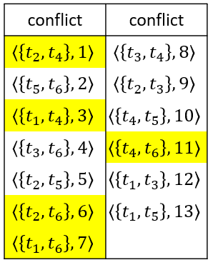
Consider a subset query on , a conflict in any is still a conflict in , and the ranking induced by any from is still ascendant. Continue with Example 4, given a range query on PR, the result set is . As shown in the figure 2, all conflicts in are yellowed faded and the ranking induced by them from is still ascendant. Let be an optimal s-repair of , then ranking could be reused to compute a -approximation of .
4.3 Fast Estimate FD-inconsistency Degree
We first settle the preprocessing method, then show an efficient implementation of the sample-and-verify method for subset queries.
4.3.1 Preprocessing
Ranking-based method mentioned above implies a pre-defined rank could be reused for the FD-inconsistency degree evaluation of every subset query result. Therefore, we discover all the conflicts in with respect to in the preprocessing step, and assign a unified rank to in advance. That is a distinct rank is assigned to each conflict as shown in figure 1(b).
Input:
An instance of a relation schema , and a set of functional dependencies
Output:
Set of conflicts in and a ascendant ranking on
Algorithm 3 illustrates the preprocessing procedure. Let be the size of . The running time of Preprocessing is at worst . Because there are at most tuple pairs of and we consider data complexity in this paper, it takes time to find out all conflicts of . And Step 7 may take time. Note that, the number of conflicts are usually not that large in practice, techniques like hash-based partition could be taken as a tool to find all possible conflicts, so that the time cost of preprocessing could be further lower, but we do not emphasis them in this paper.
4.3.2 Verification Locally
Recall the sampling-and-verification procedure, for any tuple sampled uniformly, it is to check if is in the 2-optimal s-repair of derived by given ranking . During this procedure, every conflict in eliminated in the checking procedure has a lowest rank when we turn to check it. That is, any conflict in intersecting with are either already eliminated or having a rank higher than . It is easy for the sequential implementation if we scan the ranking from its beginning. However, it is difficult without scanning the entire ranking, since the sampled tuple may not locate in the beginning.
To enable a sublinear evaluation, we need a start-from-anywhere implement method. Fortunately, the locality of a ranking can be utilized to avoid scanning the entire ranking. We employ a recursive verification starting from the conflicts involving current sampled tuple.
Basically, we begin with the sampled tuple and check the conflicts in caused by in turn from rank lowest to highest. For each conflict we currently considering, should be eliminated if one of the following conditions holds,
-
-
is lowest among all the conflicts in intersecting with it,
-
-
Every conflict in intersecting with and lower than are already known to be eliminated.
Otherwise, recursively check by the same procedure. At last, if none of conflicts in containing is decided to be eliminated, then should stay in , otherwise not, and count it into . The correctness of this method is obviously, the only concern is the running time which depends on the number of recursive calls. We next formally describe it and bound the number of recursive calls.
4.3.3 Sublinear Estimation
Algorithm 4 Fast-IncDeg performs sampling-and-verifying operations and counts the number of tuples sampled but not in by calling function NotInSR. Since is a 2-optimal s-repair of , Fast-IncDeg outcomes an -estimation of FD-inconsistency degree of .
Input:
Set of conflicts in , subset query , error
Output:
Subroutine 1 implements the verification by calling Eliminate recursively. Namely, as introduced in subsection-4.3.2, give a conflict , it considers all conflicts which include or with lower ranking. If there are no such conflicts, it returns true. Otherwise, it performs recursive calls to these conflicts in the order of their ranking. If any one-step recursion returns true, it returns false; Otherwise, it returns true. With the help of Eliminate, the subroutine 1 checks if a tuple belongs to . Concretely, it performs Eliminate on all conflicts in including in the order of their rankings, and if there exists a conflict such that Eliminate returns true, it returns true; otherwise, it returns false.
Now, we bound the number of recursive calls of Eliminate. First, we derive an important corollary from [30]. For a ranking injection of all conflicts of an instance and a tuple , let denote the number of conflicts that a call was made on in the course of the computation of . Let denote the set of all ranking injections over the conflicts of . Given a tuple , let be the number of conflicts containing . Then we define the maximum conflict number of as The average value of taken over all ranking injections and tuples is , i.e.,
| (5) |
Theorem 5
Algorithm Fast-IncDeg returns an estimate with a probability at least such that,
The average query complexity taken over all rankings , subset queries and tuples of is , where the algorithm uses only queries supported by the -oracle.
Proof.
By applying an additive Chernoff bound, suppose that it is sampled uniformly and independently tuples from , with probability more than ,
| (6) |
And with the fact that is a 2-optimal s-repair, it is obtained that,
| (7) |
For query complexity, we first bound the number of calls of . Given the result of a subset query , let be the number of tuples in , and be the number of conflicts contained in , and the maximum conflict number of . Now, consider the ranking induced by from , then equation 5 implies,
Notice that since the conflicts in is a subset of the conflicts in , for each , there are number of can produce the same ranking on the conflicts of . Group into groups , and for each and a fixed , has the same value. So we have,
The we could derive the query complexity. Let be the space of queries, then for any , we have , so that the average query complexity is that
Obviously, there are calls to sample a tuple from the result set. For each sampled tuple , the average number of calls to is . So the number of calls to is . ∎
In addition, inspired by the methodology proposed in [30], a pre-defined ranking in the preprocessing can be saved by ranking on the fly, that is, we only need to discover all conflicts in the preprocessing step and ranking whenever it is required. Since the basic idea is similar with our method, we omit the detail here, instead, we compare the two different implements in our experiments to show the efficiency of our method.
5 Experiments
This section experimentally evaluates the performace of our algorithms for OSR computing and FD-inconsistency evaluation.
5.1 Experimental Settings
All experiments are conducted on a machine with eight 16-core Intel Xeon processors and 3072GB of memory.
Dataset. We used two datasets to evaluate the performance of algorithms for OSR computing and FD-Inconsistency evaluaction experimentally.
Dataset 1: order data is an instance of the schema order shown in Example 1. Our set consists of 4 FDs taken from Example 1. To populate the relation we scraped product informations from amazon and collected real-life data: the zip and area codes for major cities and twons for all US states111http://www.geonames.org/ and street informations for all the United States222http://results.openaddresses.io/. We generated datasets of various size, ranging from 10M to 100M tuples.
Dataset 2: dblp data was extracted from dblp Bibliography333https://dblp.org/xml/. It consists of 40M tuples and the format is as follows:
Each dblp tuple contains the title of an article, the authors and the information of publication (year, publication venue, pages, electronic edition and, url) We designed 4 FDs for dblp.
To add noise to a dataset, we randomly selected an attribute of a ”correct” tuple and changed it either to a close value or to an existing value taken from another tuple. We appended such ”dirty” tuples which violate at least one or more functional dependencies to the dataset. We set a parameter ranging from to to control the noise rate.
Methods. We implemented the following algorithms: (a) the basic approximation algorithm BL LP-OSR and the improved approximation algorithm by triad elimination TE LP-OSR for OSR computing; (b) the sublinear estimation algorithm Fast-IncDeg based on two implements of -oracle for range query with and time complexity respectively, and its variation mentioned in the subsection-4.3.3 Fast-IncDeg_ol for FD-Inconsistency evaluation. Hence, there are totally 4 implements of Algorithm 4 for range query denoted by , , and respectively.
Metrics. Since a dataset with tuples is polluted by appending dirty tuples, where is noise rate, the number of tuples in the optimal repair must be larger than , i.e., . Hence, we calculate of BL LP-OSR and TE LP-OSR and use to evaluate the approximation ratio of them. What’s more, according to the definition of FD-inconsistency degree, we treat as the upper bound of FD-inconsistency degree to ensure the correctness of the Algorithm 4. To evaluate the efficiency of Algorithm 4, we issue 300 queries for each algorithm and each parameter set, and record the average of the query time.
5.2 Experimental Results
We report our findings concerning about the accuracy and efficiency of our algorithms.
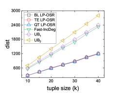
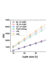
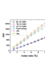
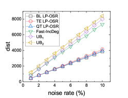
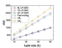
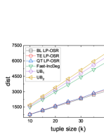
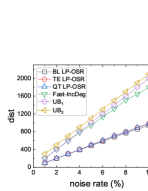
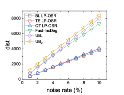
Accuracy. We first show the accuracy of BL LP-OSR, TE LP-OSR and QT LP-OSR. In figure 3, we ran them on datasets consisting of 10K to 40K tuples with noise rate ranging from to and calculated . The of BL LP-OSR, TE LP-OSR and QT LP-OSR are much less than . Because the approximation ratio only bounds the relation between worst case output of an algorithm and the optimal solution, BL LP-OSR sometimes performs better than the other two improved algorithm. What’s more, it is discovered that, after triad elimination, the ratio of 0.5 solution becomes much less since they only appear when some conflicts form a cycle with odd length.
We also evaluate the accuracy of Fast-IncDeg. We ran with parameter on the same datasets and calculated . As shown in figure 3 the value return by is less than even less than mostly since the upper bound is loose. And it is greater than the values of BL LP-OSR, TE LP-OSR and QT LP-OSR since it returns an estimate with an additive error.
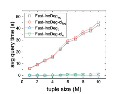
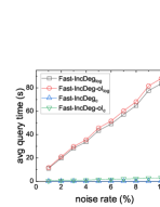
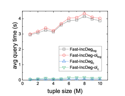
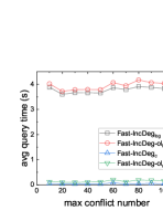
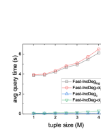
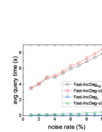
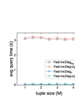
Efficiency. We evaluate the efficiency of our algorithms for FD-inconsistency evaluation. We first ran , , and on datasets with various size, noise rate ranging from to and . 300 large queries were issued per dataset and the average query time was recorded.
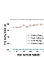
Figure 4(a), 4(b), 4(e), and 4(f) indicate that the average query time increase with the number of tuples and noise rate since both of them influence the maximum conflicts number in . Further experiments were performed to evaluate the impact of the maximum conflict number on the average query time. Since queries were generated randomly, we only bounded the maximum conflict number of the dataset . Therefore, the average query time shown in figures 4(d) and 4(h) remain basically the same with the increasing . As shown in figures 4(c) and 4(g), the average query time of and change slightly due to the impact of the number of tuples on . And the average query time of and grow with the number of tuples.
Figure 4 also illustrates that no matter how the -oracle is implemented, Fast-IncDeg performs better then Fast-IncDeg-ol. It is because that in Fast-IncDeg-ol the ranking is assigned on-the-fly when a conflict is queried and it is expensive to keep the ranking consistent in every tuple which the conflict concerned about. In addition, an efficient -oracle indeed makes the average query time drop a lot.
6 Related Work
As a principled approach managing inconsistency, Arenas et al. [5] introduced the notions of repairs to define consistent query answering. The definitions of repair differ in settings of integrity constraints and operation gain [3]. The most general form of integrity constraints are denial constraints [21], they are able to express the classic functional dependencies [1], inclusion dependencies [25], and so on. Data complexities of computing optimal repairs are widely studied in the past. The complexity of tuple-level deletion based subset repair [13, 27] is studied respectively in the past. And the complexity of cell-level update based v-repair is also studied in [27, 26]. APXcompleteness of both optimal subset repair and v-repair computation has been shown for in these works.
For the upper bound, the best approximation on subset repair is still 2 obtained by solving the corresponding vertex cover problem [27] without the limitation on the number of given FDs. For the setting of fixed number of FDs, there are still no existing algorithmic result.
For the data repairing frameworks [2], there are two kinds of works which are based on FDs, they both aim to directly resolve the inconsistency of database. One kind of methods is to repair data based on minimizing the repair cost, e.g., [5, 11, 16, 28, 34].
Given the data edit operations (including tuple-level and cell-level), minimum cost repair will output repaired data with minimizing the difference between it and the original one. But these work also do not provide us tight lower and upper bounds for data repairing. There are some other type of repairs not related with this paper, such as “minimum description length” [12], “relative trust” [10] and so on.
For inconsistency detection, there exists some detection techniques which are able to detect errors efficiently. SQL techniques for detecting FD violations were given in [13], practical algorithms for detecting violations of FDs in fragmented and distributed relations were provided in [19], and a incremental detection algorithm were proposed by [20]. In contrast to inconsistency detection, inconsistency evaluation need to compute the quantized dirtiness value of the data, rather than finding all violations.
7 Conclusions
We revisit computing an optimal s-repair problem and fast estimate of s-repair based FD-inconsistency degree of subset query results. For the lower bound, we improve the inapproximability of optimal s-repair computing problem over most cases of FDs and schemas. For the upper bound, we developed two LP-based algorithms to compute a near optimal s-repair based on different characterization of input FDs and schemas respectively. Complexity results implies it is hard to obtain a good approximation polynomially, not to mention sublinear time for large data. For the FD-inconsistency degree, we present a fast -estimation with an average sublinear query complexity, and achieve a sublinear time complexity whenever incorporating a sublinear implementation of the subset query oracle. This results give a way to estimate FD-inconsistency degree efficiently with theoretical guarantee.
References
- [1] S. Abiteboul, R. Hull, and V. Vianu. Foundations of Databases: The Logical Level. Addison-Wesley Longman Publishing Co., Inc., Boston, MA, USA, 1995.
- [2] F. N. Afrati and K. P. G. Repair checking in inconsistent databases: Algorithms and complexity. 2009.
- [3] F. N. Afrati and P. G. Kolaitis. Repair checking in inconsistent databases: Algorithms and complexity. In Proceedings of the 12th International Conference on Database Theory, ICDT 09, pages 31–41, New York, NY, USA, 2009. ACM.
- [4] O. Amini, S. Pérennes, and I. Sau. Hardness and approximation of traffic grooming. Theoretical Computer Science, 410(38-40):3751–3760, 2009.
- [5] M. Arenas, L. Bertossi, and J. Chomicki. Consistent query answers in inconsistent databases. In Proceedings of the 18th ACM Symposium on Principles of Database Systems, pages 68–79. ACM, 1999.
- [6] A. Assadi, T. Milo, and S. Novgorodov. Dance: data cleaning with constraints and experts. In 2017 IEEE 33rd International Conference on Data Engineering (ICDE), pages 1409–1410. IEEE, 2017.
- [7] M. Bergman, T. Milo, S. Novgorodov, and W.-C. Tan. Qoco: A query oriented data cleaning system with oracles. Proceedings of the VLDB Endowment, 8(12):1900–1903, 2015.
- [8] L. Bertossi. Database Repairing and Consistent Query Answering. Morgan Claypool Publishers, 2011.
- [9] L. Bertossi. Repair-based degrees of database inconsistency. In Logic Programming and Nonmonotonic Reasoning, pages 195–209. Springer, Cham, 2019.
- [10] G. Beskales, I. F. Ilyas, L. Golab, and A. Galiullin. On the relative trust between inconsistent data and inaccurate constraints. arXiv preprint arXiv:1207.5226, 2012.
- [11] P. Bohannon, W. Fan, M. Flaster, and R. Rastogi. A cost-based model and effective heuristic for repairing constraints by value modification. In Proceedings of the 2005 ACM SIGMOD international conference on Management of data, pages 143–154. ACM, 2005.
- [12] F. Chiang and R. J. Miller. A unified model for data and constraint repair. In ICDE, 2011.
- [13] J. Chomicki and J. Marcinkowski. Minimal-change integrity maintenance using tuple deletions. Inf. Comput., 197(1-2), 2005.
- [14] X. Chu, I. F. Ilyas, S. Krishnan, and J. Wang. Data cleaning: Overview and emerging challenges. In Proceedings of the 2016 International Conference on Management of Data, SIGMOD ’16, page 2201–2206, New York, NY, USA, 2016. Association for Computing Machinery.
- [15] G. Cong, W. Fan, F. Geerts, X. Jia, and S. Ma. Improving data quality: Consistency and accuracy. In Proceedings of the 33rd International Conference on Very Large Data Bases, VLDB ’07, page 315–326. VLDB Endowment, 2007.
- [16] G. Cong, W. Fan, F. Geerts, X. Jia, and S. Ma. Improving data quality: Consistency and accuracy. In Proceedings of the 33rd international conference on Very large data bases, pages 315–326. VLDB Endowment, 2007.
- [17] P. Crescenzi. A short guide to approximation preserving reductions. In Proceedings of Computational Complexity. Twelfth Annual IEEE Conference, pages 262–273. IEEE, 1997.
- [18] M. Dallachiesa, A. Ebaid, A. Eldawy, A. Elmagarmid, I. F. Ilyas, M. Ouzzani, and N. Tang. Nadeef: a commodity data cleaning system. In Proceedings of the 2013 ACM SIGMOD International Conference on Management of Data, pages 541–552. ACM, 2013.
- [19] W. Fan, F. Geerts, S. Ma, and H. Müller. Detecting inconsistencies in distributed data. 2010.
- [20] W. Fan, J. Li, N. Tang, and W. Y. qa. Incremental detection of inconsistencies in distributed data. IEEE Trans. on Knowl. and Data Eng., 26(6), 2014.
- [21] T. Gaasterland, P. Godfrey, and J. Minker. An overview of cooperative answering. Journal of Intelligent Information Systems, 1(2):123–157, 1992.
- [22] F. Geerts, G. Mecca, P. Papotti, and D. Santoro. The llunatic data-cleaning framework. Proceedings of the VLDB Endowment, 6(9):625–636, 2013.
- [23] V. Guruswami and S. Khot. Hardness of max 3sat with no mixed clauses. In Proceedings of the 20th Annual IEEE Conference on Computational Complexity, pages 154–162. IEEE Computer Society, 2005.
- [24] V. Kann. Maximum bounded 3-dimensional matching is max snp-complete. Information Processing Letters, 37(1):27–35, 1991.
- [25] H. Koehler and S. Link. Inclusion dependencies and their interaction with functional dependencies in sql. J. Comput. Syst. Sci., 85(C):104–131, 2017.
- [26] S. Kolahi and L. V. S. Lakshmanan. On approximating optimum repairs for functional dependency violations. ICDT, 2009.
- [27] E. Livshits, B. Kimelfeld, and S. Roy. Computing optimal repairs for functional dependencies. In Proceedings of the 37th ACM Symposium on Principles of Database Systems, pages 225–237. ACM, 2018.
- [28] A. Lopatenko and L. Bravo. Efficient approximation algorithms for repairing inconsistent databases. In 2007 IEEE 23rd international conference on data engineering, pages 216–225. IEEE, 2007.
- [29] G. L. Nemhauser and L. E. Trotter. Vertex packings: Structural properties and algorithms. Mathematical Programming, 8(4):232–248, 1975.
- [30] K. Onak, D. Ron, M. Rosen, and R. Rubinfeld. A near-optimal sublinear-time algorithm for approximating the minimum vertex cover size. In Proceedings of the twenty-third annual ACM-SIAM symposium on Discrete Algorithms, pages 1123–1131. Society for Industrial and Applied Mathematics, 2012.
- [31] C. D. Sa, I. F. Ilyas, B. Kimelfeld, C. Ré, and T. Rekatsinas. A formal framework for probabilistic unclean databases. In 22nd International Conference on Database Theory, ICDT 2019, March 26-28, 2019, Lisbon, Portugal, pages 6:1–6:18, 2019.
- [32] B. Salimi, L. Rodriguez, B. Howe, and D. Suciu. Interventional fairness: Causal database repair for algorithmic fairness. In Proceedings of the 2019 International Conference on Management of Data, SIGMOD ’19, page 793–810, New York, NY, USA, 2019. Association for Computing Machinery.
- [33] D. P. Williamson and D. B. Shmoys. The design of approximation algorithms. Cambridge University Press, Cambridge, England, 2011.
- [34] W. E. Winkler. Methods for evaluating and creating data quality. Information Systems, 29(7):531–550, 2004.