ZeroQ: A Novel Zero Shot Quantization Framework

Abstract

Quantization is a promising approach for reducing the inference time and memory footprint of neural networks. However, most existing quantization methods require access to the original training dataset for retraining during quantization. This is often not possible for applications with sensitive or proprietary data, e.g., due to privacy and security concerns. Existing zero-shot quantization methods use different heuristics to address this, but they result in poor performance, especially when quantizing to ultra-low precision. Here, we propose ZeroQ, a novel zero-shot quantization framework to address this. ZeroQ enables mixed-precision quantization without any access to the training or validation data. This is achieved by optimizing for a Distilled Dataset, which is engineered to match the statistics of batch normalization across different layers of the network. ZeroQ supports both uniform and mixed-precision quantization. For the latter, we introduce a novel Pareto frontier based method to automatically determine the mixed-precision bit setting for all layers, with no manual search involved. We extensively test our proposed method on a diverse set of models, including ResNet18/50/152, MobileNetV2, ShuffleNet, SqueezeNext, and InceptionV3 on ImageNet, as well as RetinaNet-ResNet50 on the Microsoft COCO dataset. In particular, we show that ZeroQ can achieve 1.71% higher accuracy on MobileNetV2, as compared to the recently proposed DFQ [32] method. Importantly, ZeroQ has a very low computational overhead, and it can finish the entire quantization process in less than 30s (0.5% of one epoch training time of ResNet50 on ImageNet). We have open-sourced the ZeroQ framework.

I Introduction

Despite the great success of deep Neural Network (NN) models in various domains, the deployment of modern NN models at the edge has been challenging due to their prohibitive memory footprint, inference time, and/or energy consumption. With the current hardware support for low-precision computations, quantization has become a popular procedure to address these challenges. By quantizing the floating point values of weights and/or activations in a NN to integers, the model size can be shrunk significantly, without any modification to the architecture. This also allows one to use reduced-precision Arithmetic Logic Units (ALUs) which are faster and more power-efficient, as compared to floating point ALUs. More importantly, quantization reduces memory traffic volume, which is a significant source of energy consumption [15].

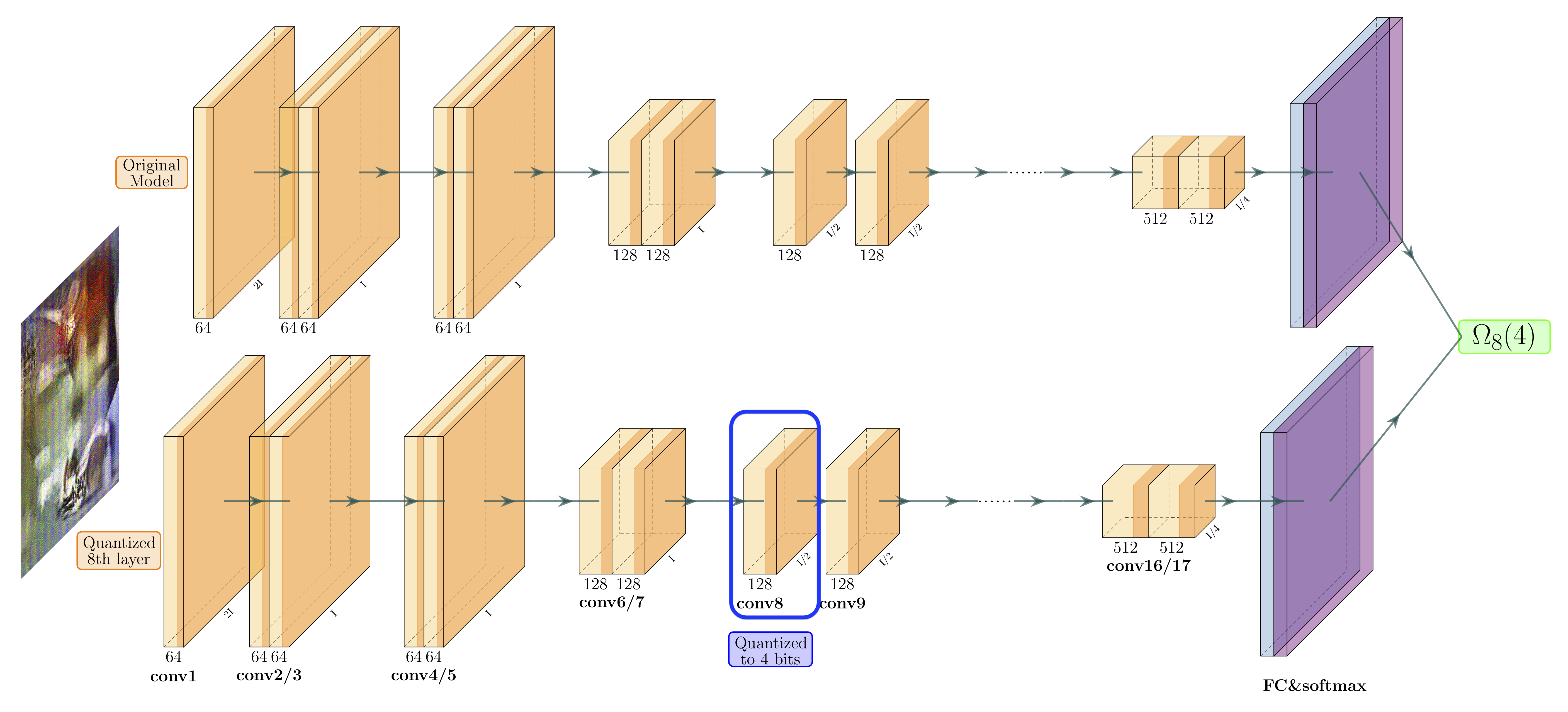
Figure 1: Illustration of sensitivity computation for ResNet18 on ImageNet. The figure shows how we compute the sensitivity of the 8-th layer when quantized to 4-bit ($\Omega_{8}(4)$) according to Eq. 2. We feed Distilled Data into the full-precision ResNet18 (top), and the same model except quantizing the 8-th layer to 4-bit (bottom) receptively. The sensitivity of the 8-th layer when quantized to 4-bit $\Omega_{8}(4)$ is defined as the KL-divergence between the output of these two models. For simplicity, we omit the residual connections here, although the same analysis is applied to the residual connections in ZeroQ.

However, quantizing a model from single precision to low-precision often results in significant accuracy degradation. One way to alleviate this is to perform the so-called quantization-aware fine-tuning [46, 34, 5, 42, 45, 18] to reduce the performance gap between the original model and the quantized model. Basically, this is a retraining procedure that is performed for a few epochs to adjust the NN parameters to reduce accuracy drop. However, quantization-aware fine-tuning can be computationally expensive and time-consuming. For example, in online learning situations, where a model needs to be constantly updated on new data and deployed every few hours, there may not be enough time for the fine-tuning procedure to finish. More importantly, in many real-world scenarios, the training dataset is sensitive or proprietary, meaning that it is not possible to access the dataset that was used to train the model. Good examples are medical data, bio-metric data, or user data used in recommendation systems.

To address this, recent work has proposed post-training quantization [19, 32, 44, 3], which directly quantizes NN models without fine-tuning. However, as mentioned above, these methods result in non-trivial performance degradation, especially for low-precision quantization. Furthermore, previous post-training quantization methods usually require limited (unlabeled) data to assist the post-training quantization. However, for cases such as MLaaS (e.g., Amazon AWS and Google Cloud), it may not be possible to access any of the training data from users. An example application case is health care information which cannot be uploaded to the cloud due to various privacy issues and/or regulatory constraints. Another shortcoming is that often post-quantization methods [30, 44, 3] only focus on standard NNs such as ResNet [13] and InceptionV3 [38] for image classification, and they do not consider more demanding tasks such as object detection.

In this work, we propose ZeroQ, a novel zero-shot quantization scheme to overcome the issues mentioned above. In particular, ZeroQ allows quantization of NN models, without any access to any training/validation data. It uses a novel approach to automatically compute a mixed-precision configuration without any expensive search. In particular, our contributions are as follows.

• We propose an optimization formulation to generate Distilled Data, i.e., synthetic data engineered to match the statistics of batch normalization layers. This reconstruction has a small computational overhead. For example, it only takes 3s (0.05% of one epoch training time) to generate 32 images for ResNet50 on ImageNet on an 8-V100 system.

• We use the above reconstruction framework to perform sensitivity analysis between the quantized and the original model. We show that the Distilled Data matches the sensitivity of the original training data (see Figure 1 and Table IV for details). We then use the Distilled Data, instead of original/real data, to perform post-training quantization. The entire sensitivity computation here only costs 12s (0.2% of one epoch training time) in total for ResNet50. Importantly, we never use any training/validation data for the entire process.

• Our framework supports both uniform and mixed-precision quantization. For the latter, we propose a novel automatic precision selection method based on a Pareto frontier optimization (see Figure 4 for illustration). This is achieved by computing the quantization sensitivity based on the Distilled Data with small computational overhead. For example, we are able to determine automatically the mixed-precision setting in under 14s for ResNet50.

We extensively test our proposed ZeroQ framework on a wide range of NNs for image classification and object detection tasks, achieving state-of-the-art quantization results in all tests. In particular, we present quantization results for both standard models (e.g., ResNet18/50/152 and InceptionV3) and efficient/compact models (e.g., MobileNetV2, ShuffleNet, and SqueezeNext) for image classification task. Importantly, we also test ZeroQ for object detection on Microsoft COCO dataset [28] with RetinaNet [27]. Among other things, we show that ZeroQ achieves 1.71% higher accuracy on MobileNetV2 as compared to the recently proposed DFQ [32] method.

II Related work

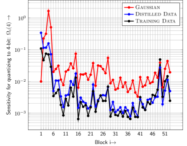
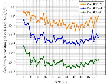
Figure 2: (Left) Sensitivity of each layer in ResNet50 when quantized to 4-bit weights, measured with different kinds of data (red for Gaussian, blue for Distilled Data, and black for training data). (Right) Sensitivity of ResNet50 when quantized to 2/4/8-bit weight precision (measured with Distilled Data).

Here we provide a brief (and by no means extensive) review of the related work in literature. There is a wide range of methods besides quantization which have been proposed to address the prohibitive memory footprint and inference latency/power of modern NN architectures. These methods are typically orthogonal to quantization, and they include efficient neural architecture design [17, 9, 16, 36, 43], knowledge distillation [14, 35], model pruning [11, 29, 24], and hardware and NN co-design [9, 21]. Here we focus on quantization [2, 6, 34, 41, 23, 48, 45, 46, 5, 8, 42], which compresses the model by reducing the bit precision used to represent parameters and/or activations. An important challenge with quantization is that it can lead to significant performance degradation, especially in ultra-low bit precision settings. To address this, existing methods propose quantization-aware fine-tuning to recover lost performance [20, 18, 4]. Importantly, this requires access to the full dataset that was used to train the original model. Not only can this be very time-consuming, but often access to training data is not possible.

To address this, several papers focused on developing post-training quantization methods (also referred to as post-quantization), without any fine-tuning/training. In particular, [19] proposes the OMSE method to optimize the $L_{2}$ distance between the quantized tensor and the original tensor. Moreover, [3] proposed the so-called ACIQ method to analytically compute the clipping range, as well as the per-channel bit allocation for NNs, and it achieves relatively good testing performance. However, they use per-channel quantization for activations, which is difficult for efficient hardware implementation in practice. In addition, [44] proposes an outlier channel splitting (OCS) method to solve the outlier channel problem. However, these methods require access to limited data to reduce the performance drop [19, 3, 44, 30, 22].

The recent work of [32] proposed Data Free Quantization (DFQ). It further pushes post-quantization to zero-shot scenarios, where neither training nor testing data are accessible during quantization. The work of [32] uses a weight equalization scheme [30] to remove outliers in both weights and activations, and they achieve similar results with layer-wise quantization, as compared to previous post-quantization work with channel-wise quantization [20]. However, [32] their performance significantly degrades when NNs are quantized to 6-bit or lower.

A recent concurrent paper to ours independently proposed to use Batch Normalization statistics to reconstruct input data [12]. They propose a knowledge-distillation based method to boost the accuracy further, by generating input data that is similar to the original training dataset, using the so-called Inceptionism [31]. However, it is not clear how the latter approach can be used for tasks such as object detection or image segmentation. Furthermore, this knowledge-distillation process adds to the computational time required for zero-shot quantization. As we will show in our work, it is possible to use batch norm statistics combined with mixed-precision quantization to achieve state-of-the-art accuracy, and importantly this approach is not limited to image classification task. In particular, we will present results on object detection using RetinaNet-ResNet50, besides testing ZeroQ on a wide range of models for image classification (using ResNet18/50/152, MobileNetV2, ShuffleNet, SqueezeNext, and InceptionV3), We show that for all of these cases ZeroQ exceeds state-of-the-art quantization performance. Importantly, our approach has a very small computational overhead. For example, we can finish ResNet50 quantization in under 30 seconds on an 8 V-100 system (corresponding to 0.5% of one epoch training time of ResNet50 on ImageNet).

Directly quantizing all NN layers to low precision can lead to significant accuracy degradation. A promising approach to address this is to perform mixed-precision quantization [8, 7, 40, 47, 39], where different bit-precision is used for different layers. The key idea behind mixed-precision quantization is that not all layers of a convolutional network are equally “sensitive” to quantization. A naïve mixed-precision quantization method can be computationally expensive, as the search space for determining the precision of each layer is exponential in the number of layers. To address this, [39] uses NAS/RL-based search algorithm to explore the configuration space. However, these searching methods can be expensive and are often sensitive to the hyper-parameters and the initialization of the RL based algorithm. Alternatively, the recent work of [8, 37, 7] introduces a Hessian based method, where the bit precision setting is based on the second-order sensitivity of each layer. However, this approach does require access to the original training set, a limitation which we address in ZeroQ.

III Methodology

For a typical supervised computer vision task, we seek to minimize the empirical risk loss, i.e.,

$$\min_{\theta}\mathcal{L}(\theta)=\frac{1}{N}\sum_{i=1}^{N}f(\mathcal{M}(\theta;x_{i}),y_{i}),$$ (1)

where $\theta\in{\mathbb{R}}^{n}$ is the learnable parameter, $f(\cdot,\cdot)$ is the loss function (typically cross-entropy loss), $(x_{i},y_{i})$ is the training input/label pair, $\mathcal{M}$ is the NN model with $L$ layers, and $N$ is the total number of training data points. Here, we assume that the input data goes through standard preprocessing normalization of zero mean ($\mu_{0}=0$) and unit variance ($\sigma_{0}=1$). Moreover, we assume that the model has $L$ BN layers denoted as $BN_{1}$, $BN_{2}$, …, $BN_{L}$. We denote the activations before the i-th BN layer with $z_{i}$ (in other words $z_{i}$ is the output of the i-th convolutional layer). During inference, $z_{i}$ is normalized by the running mean ($\mu_{i}$) and variance ($\sigma_{i}^{2}$) of parameters in the i-th BN layer ($BN_{i}$), which is pre-computed during the training process. Typically BN layers also include scaling and bias correction, which we denote as $\gamma_{i}$ and $\beta_{i}$, respectively.

We assume that before quantization, all the NN parameters and activations are stored in 32-bit precision and that we have no access to the training/validation datasets. To quantize a tensor (either weights or activations), we clip the parameters to a range of $[a,b]$ ($a,b\in{\mathbb{R}}$), and we uniformly discretize the space to $2^{k}-1$ even intervals using asymmetric quantization. That is, the length of each interval will be $\Delta=\frac{b-a}{2^{k}-1}$. As a result, the original 32-bit single-precision values are mapped to unsigned integers within the range of $[0,2^{k}-1]$. Some work has proposed non-uniform quantization schemes which can capture finer details of weight/activation distribution [33, 10, 42]. However, we only use asymmetric uniform quantization, as the non-uniform methods are typically not suitable for efficient hardware execution.

The ZeroQ framework supports both fixed-precision and mixed-precision quantization. In the latter scheme, different layers of the model could have different bit precisions (different $k$). The main idea behind mixed-precision quantization is to keep more sensitive layers at higher precision, and more aggressively quantize less sensitive layers, without increasing overall model size. As we will show later, this mixed-precision quantization is key to achieving high accuracy for ultra-low precision settings such as 4-bit quantization. Typical choices for $k$ for each layer are $\{2,4,8\}$ bit. Note that this mixed-precision quantization leads to exponentially large search space, as every layer could have one of these bit precision settings. It is possible to avoid this prohibitive search space if we could measure the sensitivity of the model to the quantization of each layer [8, 37, 7]. For the case of post-training quantization (i.e. without fine-tuning), a good sensitivity metric is to use Kullback–Leibler (KL) divergence between the original model and the quantized model, defined as:

$$\Omega_{i}(k)=\frac{1}{N}\sum_{j=1}^{N_{dist}}\textsc{KL}(\mathcal{M}(\theta;x_{j}),\mathcal{M}(\tilde{\theta}_{i}(\textit{k-bit});x_{j})).$$ (2)

where $\Omega_{i}(k)$ measures how sensitive the $i$-th layer is when quantized to k-bit, and $\tilde{\theta}_{i}(\textit{k-bit})$ refers to quantized model parameters in the $i$-th layer with $k$-bit precision. If $\Omega_{i}(k)$ is small, the output of the quantized model will not significantly deviate from the output of the full precision model when quantizing the $i$-th layer to $k$-bits, and thus the $i$-th layer is relatively insensitive to k-bit quantization, and vice versa. This process is schematically shown in Figure 1 for ResNet18. However, an important problem is that for zero-shot quantization we do not have access to the original training dataset $x_{j}$ in Eq. 2. We address this by “distilling” a synthetic input data to match the statistics of the original training dataset, which we refer to as Distilled Data. We obtain the Distilled Data by solely analyzing the trained model itself, as described below.

III-A Distilled Data

For zero-shot quantization, we do not have access to any of the training/validation data. This poses two challenges. First, we need to know the range of values for activations of each layer so that we can clip the range for quantization (the $[a,b]$ range mentioned above). However, we cannot determine this range without access to the training dataset. This is a problem for both uniform and mixed-precision quantization. Second, another challenge is that for mixed-precision quantization, we need to compute $\Omega_{i}$ in Eq. 2, but we do not have access to training data $x_{j}$. A very naïve method to address these challenges is to create a random input data drawn from a Gaussian distribution with zero mean and unit variance and feed it into the model. However, this approach cannot capture the correct statistics of the activation data corresponding to the original training dataset. This is illustrated in Figure 2 (left), where we plot the sensitivity of each layer of ResNet50 on ImageNet measured with the original training dataset (shown in black) and Gaussian based input data (shown in red). As one can see, the Gaussian data clearly does not capture the correct sensitivity of the model. For instance, for the first three layers, the sensitivity order of the red line is actually the opposite of the original training data.

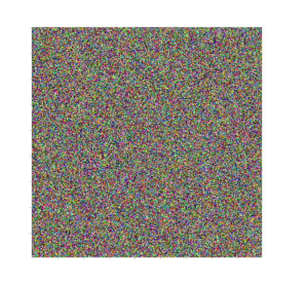
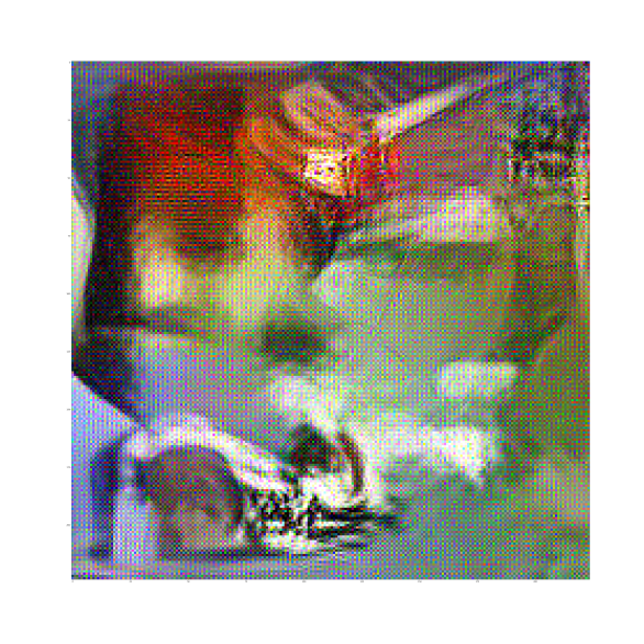
Figure 3: Visualization of Gaussian data (left) and Distilled Data (right). More local structure can be seen in our Distilled Data that is generated according to Algorithm 1.

To address this problem, we propose a novel method to “distill” input data from the NN model itself, i.e., to generate synthetic data carefully engineered based on the properties of the NN. In particular, we solve a distillation optimization problem, in order to learn an input data distribution that best matches the statistics encoded in the BN layer of the model. In more detail, we solve the following optimization problem:

$$\min_{x^{r}}\sum_{i=0}^{L}\|\tilde{\mu}_{i}^{r}-\mu_{i}\|_{2}^{2}+\|\tilde{\sigma}_{i}^{r}-\sigma_{i}\|_{2}^{2},$$ (3)

where $x^{r}$ is the reconstructed (distilled) input data, and $\mu_{i}^{r}$/$\sigma_{i}^{r}$ are the mean/standard deviation of the Distilled Data’s distribution at layer $i$, and $\mu_{i}$/$\sigma_{i}$ are the corresponding mean/standard deviation parameters stored in the BN layer at layer $i$. In other words, after solving this optimization problem, we can distill an input data which, when fed into the network, can have a statistical distribution that closely matches the original model. Please see Algorithm 1 for a description. This Distilled Data can then be used to address the two challenges described earlier. First, we can use the Distilled Data’s activation range to determine quantization clipping parameters (the $[a,b]$ range mentioned above). Note that some prior work [3, 22, 44] address this by using limited (unlabeled) data to determine the activation range. However, this contradicts the assumptions of zero-shot quantization, and may not be applicable for certain applications. Second, we can use the Distilled Data and feed it in Eq. 2 to determine the quantization sensitivity ($\Omega_{i}$). The latter is plotted for ResNet50 in Figure 2 (left) shown in solid blue color. As one can see, the Distilled Data closely matches the sensitivity of the model as compared to using Gaussian input data (shown in red). We show a visualization of the random Gaussian data as well as the Distilled Data for ResNet50 in Figure 3. We can see that the Distilled Data can capture fine-grained local structures.

Input: Model: $\mathcal{M}$ with $L$ Batch Normalization layers

Output: A batch of distilled data: $x^{r}$

Generate random data from Gaussian: $x^{r}$

Get $\mu_{i},\sigma_{i}$ from Batch Normalization layers of $\mathcal{M}$, $i\in{0,~{}1,~{}\dots,~{}L}$

  // Note that $\mu_{0}=0,~{}\sigma_{0}=1$

for j $=1,2,\ldots$ do

       Forward propagate $\mathcal{M}(x^{r})$ and gather intermediate activations

      Get $\tilde{\mu}_{i}$ and $\tilde{\sigma}_{i}$ from intermediate activations, $i\in{1,~{}\dots,~{}n}$

      Compute $\tilde{\mu}_{0}$ and $\tilde{\sigma}_{0}$ of $x^{r}$

      Compute the loss based on Eq. 3

      Backward propagate and update $x^{r}$

Algorithm 1 Generation of Distilled Data

III-B Pareto Frontier

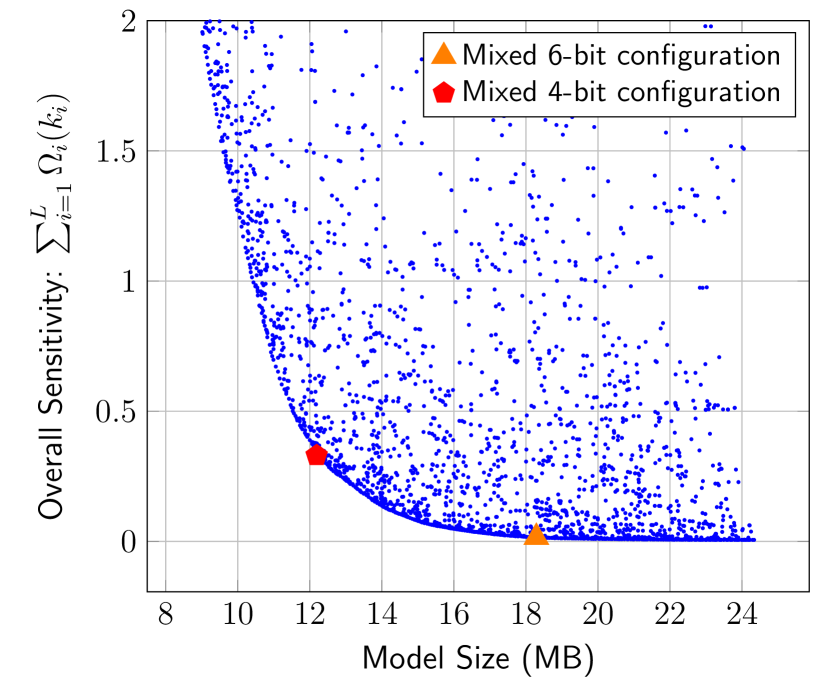
Figure 4: The Pareto frontier of ResNet50 on ImageNet. Each point shows a mixed-precision bit setting. The x-axis shows the resulting model size for each configuration, and the y-axis shows the resulting sensitivity. In practice, a constraint for model size is set. Then the Pareto frontier method chooses a bit-precision configuration that results in minimal perturbation. We show two examples for 4 and 6-bit mixed precision configuration shown in red and orange. The corresponding results are presented in Table Ia.

As mentioned before, the main challenge for mixed-precision quantization is to determine the exact bit precision configuration for the entire NN. For an L-layer model with $m$ possible precision options, the mixed-precision search space, denoted as $\mathcal{S}$, has an exponential size of $m^{L}$. For example for ResNet50 with just three bit precision of $\{2,4,8\}$ (i.e., $m=3$), the search space contains $7.2\times 10^{23}$ configurations. However, we can use the sensitivity metric in Eq. 2 to reduce this search space. The main idea is to use higher bit precision for layers that are more sensitive, and lower bit precision for layers that are less sensitive. This gives us a relative ordering on the number of bits. To compute the precise bit precision setting, we propose a Pareto frontier approach similar to the method used in [7].

The Pareto frontier method works as follows. For a target quantized model size of $S_{target}$, we measure the overall sensitivity of the model for each bit precision configuration that results in the $S_{target}$ model size. We choose the bit-precision setting that corresponds to the minimum overall sensitivity. In more detail, we solve the following optimization problem:

$$\min_{\{k_{i}\}_{i=1}^{L}}\Omega_{sum}=\sum_{i=1}^{L}\Omega_{i}(k_{i})~{}~{}s.t.~{}\sum_{i=1}^{L}P_{i}*k_{i}\leq S_{target},$$ (4)

where $k_{i}$ is the quantization precision of the i-th layer, and $P_{i}$ is the parameter size for the $i$-th layer. Note that here we make the simplifying assumption that the sensitivity of different layers are independent of the choice of bits for other layers (hence $\Omega_{i}$ only depends on the bit precision for the $i$-th layer). Using a dynamic programming method we can solve the best setting with different $S_{target}$ together, and then we plot the Pareto frontier. An example is shown in Figure 4 for ResNet50 model, where the x-axis is the model size for each bit precision configuration, and the y-axis is the overall model perturbation/sensitivity. Each blue dot in the figure represents a mixed-precision configuration. In ZeroQ, we choose the bit precision setting that has the smallest perturbation with a specific model size constraint.

Importantly, note that the computational overhead of computing the Pareto frontier is $\mathcal{O}(mL)$. This is because we compute the sensitivity of each layer separately from other layers. That is, we compute sensitivity $\Omega_{i}$ ($i=1,2,...,L$) with respect to all $m$ different precision options, which leads to the $\mathcal{O}(mL)$ computational complexity. We should note that this Pareto Frontier approach (including the Dynamic Programming optimizer), is not theoretically guaranteed to result in the best possible configuration, out of all possibilities in the exponentially large search space. However, our results show that the final mixed-precision configuration achieves state-of-the-art accuracy with small performance loss, as compared to the original model in single precision.

TABLE I: Quantization results of ResNet50, MobileNetV2, and ShuffleNet on ImageNet. We abbreviate quantization bits used for weights as “W-bit” (for activations as “A-bit”), top-1 test accuracy as “Top-1.” Here, “MP” refers to mixed-precision quantization, “No D” means that none of the data is used to assist quantization, and “No FT” stands for no fine-tuning (re-training). Compared to post-quantization methods OCS [44], OMSE [19], and DFQ [32], ZeroQ achieves better accuracy. $\text{{ZeroQ}}^{\dagger}$ means using percentile for quantization.

Method	No D	No FT	W-bit	A-bit	Size (MB)	Top-1
Baseline	–	–	32	32	97.49	77.72
OMSE [19]	✓	✓	4	32	12.28	70.06
OMSE [19]	✗	✓	4	32	12.28	74.98
PACT [5]	✗	✗	4	4	12.19	76.50
ZeroQ	✓	✓	MP	8	12.17	75.80
$\text{{ZeroQ}}^{\dagger}$	✓	✓	MP	8	12.17	76.08
OCS [44]	✗	✓	6	6	18.46	74.80
ZeroQ	✓	✓	MP	6	18.27	77.43
ZeroQ	✓	✓	8	8	24.37	77.67

(a) ResNet50

Method	No D	No FT	W-bit	A-bit	Size (MB)	Top-1
Baseline	–	–	32	32	13.37	73.03
ZeroQ	✓	✓	MP	8	1.67	68.83
$\text{{ZeroQ}}^{\dagger}$	✓	✓	MP	8	1.67	69.44
Integer-Only [18]	✗	✗	6	6	2.50	70.90
ZeroQ	✓	✓	MP	6	2.50	72.85
RVQuant [33]	✗	✗	8	8	3.34	70.29
DFQ [32]	✓	✓	8	8	3.34	71.20
ZeroQ	✓	✓	8	8	3.34	72.91

(b) MobileNetV2

Method	No D	No FT	W-bit	A-bit	Size (MB)	Top-1
Baseline	–	–	32	32	5.94	65.07
ZeroQ	✓	✓	MP	8	0.74	58.96
ZeroQ	✓	✓	MP	6	1.11	62.90
ZeroQ	✓	✓	8	8	1.49	64.94

(c) ShuffleNet

IV Results

In this section, we extensively test ZeroQ on a wide range of models and datasets. We first start by discussing the zero-shot quantization of ResNet18/50, MobileNet-V2, and ShuffleNet on ImageNet in Section IV-A. Additional results for quantizing ResNet152, InceptionV3, and SqueezeNext on ImageNet, as well as ResNet20 on Cifar10 are provided in Appendix -C. We also present results for object detection using RetinaNet tested on Microsoft COCO dataset in Section IV-B. We emphasize that all of the results achieved by ZeroQ are 100% zero-shot without any need for fine-tuning.

We also emphasize that we used exactly the same hyper-parameters (e.g., the number of iterations to generate Distilled Data) for all experiments, including the results on Microsoft COCO dataset.

IV-A ImageNet

We start by discussing the results on the ImageNet dataset. For each model, after generating Distilled Data based on Eq. 3, we compute the sensitivity of each layer using Eq. 2 for different bit precision. Next, we use Eq. 4 and the Pareto frontier introduced in Section III-B to get the best bit-precision configuration based on the overall sensitivity for a given model size constraint. We denote the quantized results as WwAh where w and h denote the bit precision used for weights and activations of the NN model.

We present zero-shot quantization results for ResNet50 in Table Ia. As one can see, for W8A8 (i.e., 8-bit quantization for both weights and activations), ZeroQ results in only 0.05% accuracy degradation. Further quantizing the model to W6A6, ZeroQ achieves 77.43% accuracy, which is 2.63% higher than OCS [44], even though our model is slightly smaller (18.27MB as compared to 18.46MB for OCS). We show that we can further quantize ResNet50 down to just 12.17MB with mixed precision quantization, and we obtain 75.80% accuracy. Note that this is 0.82% higher than OMSE [19] with access to training data and 5.74% higher than zero-shot version of OMSE. Importantly, note that OMSE keeps activation bits at 32-bits, while for this comparison our results use 8-bits for the activation (i.e., $4\times$ smaller activation memory footprint than OMSE). For comparison, we include results for PACT [5], a standard quantization method that requires access to training data and also requires fine-tuning.

An important feature of the ZeroQ framework is that it can perform the quantization with very low computational overhead. For example, the end-to-end quantization of ResNet50 takes less than 30 seconds on an 8 Tesla V100 GPUs (one epoch training time on this system takes 100 minutes). In terms of timing breakdown, it takes 3s to generate the Distilled Data, 12s to compute the sensitivity for all layers of ResNet50, and 14s to perform Pareto Frontier optimization.

We also show ZeroQ results on MobileNetV2 and compare it with both DFQ [32] and fine-tuning based methods [33, 18], as shown in Table Ib. For W8A8, ZeroQ has less than 0.12% accuracy drop as compared to baseline, and it achieves 1.71% higher accuracy as compared to DFQ method.

Further compressing the model to W6A6 with mixed-precision quantization for weights, ZeroQ can still outperform Integer-Only [18] by 1.95% accuracy, even though ZeroQ does not use any data or fine-tuning. ZeroQ can achieve 68.83% accuracy even when the weight compression is 8$\times$, which corresponds to using 4-bit quantization for weights on average.

We also experimented with percentile based clipping to determine the quantization range [25] (please see Section -D for details). The results corresponding to percentile based clipping are denoted as $ZeroQ^{\dagger}$ and reported in Table I. We found that using percentile based clipping is helpful for low precision quantization. Other choices for clipping methods have been proposed in the literature. Here we note that our approach is orthogonal to these improvements and that ZeroQ could be combined with these methods.

We also apply ZeroQ to quantize efficient and highly compact models such as ShuffleNet, whose model size is only 5.94MB. To the best of our knowledge, there exists no prior zero-shot quantization results for this model. ZeroQ achieves a small accuracy drop of 0.13% for W8A8. We can further quantize the model down to an average of 4-bits for weights, which achieves a model size of only 0.73MB, with an accuracy of 58.96%.

TABLE II: Object detection on Microsoft COCO using RetinaNet. By keeping activations to be 8-bit, our 4-bit weight result is comparable with recently proposed method FQN [25], which relies on fine-tuning. (Note that FQN uses 4-bit activations and the baseline used in [25] is 35.6 mAP).

Method	No D	No FT	W-bit	A-bit	Size (MB)	mAP
Baseline	✓	✓	32	32	145.10	36.4
FQN [25]	✗	✗	4	4	18.13	32.5
ZeroQ	✓	✓	MP	8	18.13	33.7
ZeroQ	✓	✓	MP	6	24.17	35.9
ZeroQ	✓	✓	8	8	36.25	36.4

We also compare with the recent Data-Free Compression (DFC) [12] method. There are two main differences between ZeroQ and DFC. First, DFC proposes a fine-tuning method to recover accuracy for ultra-low precision cases. This can be time-consuming and as we show it is not necessary. In particular, we show that with mixed-precision quantization one can actually achieve higher accuracy without any need for fine-tuning. This is shown in Table III for ResNet18 quantization on ImageNet. In particular, note the results for W4A4, where the DFC method without fine-tuning results in more than 15% accuracy drop with a final accuracy of 55.49%. For this reason, the authors propose a method with post quantization training, which can boost the accuracy to 68.05% using W4A4 for intermediate layers, and 8-bits for the first and last layers. In contrast, ZeroQ achieves a higher accuracy of 69.05% without any need for fine-tuning. Furthermore, the end-to-end zero-shot quantization of ResNet18 takes only 12s on an 8-V100 system (equivalent to $0.4\%$ of the 45 minutes time for one epoch training of ResNet18 on ImageNet). Secondly, DFC method uses Inceptionism [31] to facilitate the generation of data with random labels, but it is hard to extend this for object detection and image segmentation tasks.

TABLE III: Uniform post-quantization on ImageNet with ResNet18. We use percentile clipping for W4A4 and W4A8 settings. $\text{{ZeroQ}}^{\dagger}$ means using percentile for quantization.

Method	No D	No FT	W-bit	A-bit	Size (MB)	Top-1
Baseline	–	–	32	32	44.59	71.47
PACT [5]	✗	✗	4	4	5.57	69.20
DFC [12]	✓	✓	4	4	5.58	55.49
DFC [12]	✓	✗	4	4	5.58	68.06
ZeroQ	✓	✓	MP	4	5.57	–
$\text{{ZeroQ}}^{\dagger}$	✓	✓	MP	4	5.57	69.05
Integer-Only[18]	✗	✗	6	6	8.36	67.30
DFQ [32]	✓	✓	6	6	8.36	66.30
ZeroQ	✓	✓	MP	6	8.35	71.30
RVQuant [33]	✗	✗	8	8	11.15	70.01
DFQ [32]	✓	✓	8	8	11.15	69.70
DFC [12]	✓	✗	8	8	11.15	69.57
ZeroQ	✓	✓	8	8	11.15	71.43

We include additional results of quantized ResNet152, InceptionV3, and SqueezeNext on ImageNet, as well as ResNet20 on Cifar10, in Appendix -C.

IV-B Microsoft COCO

Object detection is often much more complicated than ImageNet classification. To demonstrate the flexibility of our approach we also test ZeroQ on an object detection task on Microsoft COCO dataset. RetinaNet [27] is a state-of-the-art single-stage detector, and we use the pretrained model with ResNet50 as the backbone, which can achieve 36.4 mAP.

One of the main difference of RetinaNet with previous NNs we tested on ImageNet is that some convolutional layers in RetinaNet are not followed by BN layers. This is because of the presence of a feature pyramid network (FPN) [26], and it means that the number of BN layers is slightly smaller than that of convolutional layers. However, this is not a limitation and the ZeroQ framework still works well. Specifically, we extract the backbone of RetinaNet and create Distilled Data. Afterwards, we feed the Distilled Data into RetinaNet to measure the sensitivity as well as to determine the activation range for the entire NN. This is followed by optimizing for the Pareto Frontier, discussed earlier.

The results are presented in Table II. We can see that for W8A8 ZeroQ has no performance degradation. For W6A6, ZeroQ achieves 35.9 mAP. Further quantizing the model to an average of 4-bits for the weights, ZeroQ achieves 33.7 mAP. Our results are comparable to the recent results of FQN [25], even though it is not a zero-shot quantization method (i.e., it uses the full training dataset and requires fine-tuning). However, it should be mentioned that ZeroQ keeps the activations to be 8-bits, while FQN uses 4-bit activations.

V Ablation Study

Here, we present an ablation study for the two components of ZeroQ: (i) the Distilled Data generated by Eq. 3 to help sensitivity analysis and determine activation clipping range; and (ii) the Pareto frontier method for automatic bit-precision assignment. Below we discuss the ablation study for each part separately.

V-A Distilled Data

In this work, all the sensitivity analysis and the activation range are computed on the Distilled Data. Here, we perform an ablation study on the effectiveness of Distilled Data as compared to using just Gaussian data. We use three different types of data sources, (i) Gaussian data with mean “0” and variance “1”, (ii) data from training dataset, (iii) our Distilled Data, as the input data to measure the sensitivity and to determine the activation range. We quantize ResNet50 and MobileNetV2 to an average of 4-bit for weights and 8-bit for activations, and we report results in Table IV.

For ResNet50, using training data results in 75.95% testing accuracy. With Gaussian data, the performance degrades to 75.44%. ZeroQ can alleviate the gap between Gaussian data and training data and achieves 75.80%. For more compact/efficient models such as MobileNetV2, the gap between using Gaussian data and using training data increases to 2.33%. ZeroQ can still achieve 68.83%, which is only 0.23% lower than using training data. Additional results for ResNet18, ShuffleNet and SqueezeNext are shown in Table VIII.

TABLE IV: Ablation study for Distilled Data on ResNet50 and MobileNetv2. We show the performance of ZeroQ with different data to compute the sensitivity and to determine the activation range. All quantized models have the same size as models with 4-bit weights and 8-bit activations.

Method	W-bit	A-bit	ResNet50	MobileNetV2
Baseline	32	32	77.72	73.03
Gaussian	MP	8	75.44	66.73
Training Data	MP	8	75.95	69.06
Distilled Data	MP	8	75.80	68.83

V-B Sensitivity Analysis

Here, we perform an ablation study to show that the bit precision of the Pareto frontier method works well. To test this, we compare ZeroQ with two cases, one where we choose a bit-configuration that corresponds to maximizing $\Omega_{sum}$ (which is opposite to the minimization that we do in ZeroQ), and one case where we use random bit precision for different layers. We denote these two methods as Inverse and Random. The results for quantizing weights to an average of 4-bit and activations to 8-bit are shown in Table V. We report the best and worst testing accuracy as well as the mean and variance in the results out of 20 tests. It can be seen that ZeroQ results in significantly better testing performance as compared to Inverse and Random. Another noticeable point is that the best configuration (i.e., minimum $\Omega_{sum}$) can outperform 0.18% than the worst case among the top-20 configurations from ZeroQ, which reflects the advantage of the Pareto frontier method. Also, notice the small variance of all configurations generated by ZeroQ.

TABLE V: Ablation study for sensitivity analysis on ImageNet (W4A8) with ResNet50. Top-20 configurations are selected based on different sensitivity metric types. We report the best, mean, and worst accuracy among 20 configurations. “ZeroQ” and “Inverse” mean selecting the bit configurations to minimize and maximize the overall sensitivity, respectively, under the average 4-bit weight constraint. “Random” means randomly selecting the bit for each layer and making the total size equivalent to 4-bit weight quantization.

	Top-1 Accuracy
Baseline	77.72
Uniform	66.59
	Best	Worst	Mean	Var
Random	38.98	0.10	6.86	105.8
Inverse	0.11	0.06	0.07	3.0$\times 10^{-4}$
ZeroQ	75.80	75.62	75.73	2.4$\bf{\times 10^{-3}}$

VI Conclusions

We have introduced ZeroQ, a novel post-training quantization method that does not require any access to the training/validation data. Our approach uses a novel method to distill an input data distribution to match the statistics in the batch normalization layers of the model. We show that this Distilled Data is very effective in capturing the sensitivity of different layers of the network. Furthermore, we present a Pareto frontier method to select automatically the bit-precision configuration for mixed-precision settings. An important aspect of ZeroQ is its low computational overhead. For example, the end-to-end zero-shot quantization time of ResNet50 is less than 30 seconds on an 8-V100 GPU system. We extensively test ZeroQ on various datasets and models. This includes various ResNets, InceptionV3, MobileNetV2, ShuffleNet, and SqueezeNext on ImageNet, ResNet20 on Cifar10, and even RetinaNet for object detection on Microsoft COCO dataset. We consistently achieve higher accuracy with the same or smaller model size compared to previous post-training quantization methods. All results show that ZeroQ could exceed previous zero-shot quantization methods. We have open sourced ZeroQ framework [1].

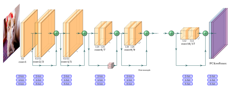
Figure 5: Mixed precision illustration of ResNet18 on ImageNet.

-A Pareto Frontier

In Section III-B, we presented how we compute the overall sensitivity incurred by performing mixed-precision quantization. In particular, in Eq. 4 we made the simplifying assumption that the sensitivity of each layer to quantization is independent to sensitivity of other layers (we refer to this as independence assumption). This is clearly not the case in practice. One can instead directly compute the sensitivity for each possible bit-precision computation without any approximation but this is not possible as there are $m^{L}$ possible bit-precision configurations. Here we discuss our approach which falls in between these two extremes. Instead of computing the sensitivity of the entire network at once, we break the network into $L/a$ groups, with each group containing $a$ layers. Furthermore, we break the x-axis (model size) of the Pareto frontier plot into $b$ intervals in every steps mentioned below.

We start with the first $a$ layers of the network. We compute the sensitivity of these layers with the independence assumption. This means we only have to compute $m\times a$ sensitivities. Afterwards, for each interval on the x-axis, we choose top $\tilde{t}$ configurations that have the lowest overall sensitivity when the first $a$ layers are quantized. We then relax the independence assumption for these $\tilde{t}$ configurations and recompute the overall sensitivity, $\Omega_{sum}$, without any approximation. This leads to a cost of $\tilde{t}$ of computing Eq. 4. We then select the top $t$ configurations out of these. We conduct this process for all the $b$ intervals for the model size. Therefore, the total cost will be $\tilde{t}\times b$.

The next step is to consider the next set of $a$ layers. This is similar to the algorithm for the first step, except that now we need to consider the top $t\times b$ configurations selected for the first $a$ layers. We first make the independence assumption for the second $a$ layers. Then we choose top $\tilde{t}\times b$ configurations out of all $t\times b\times m^{a}$ possible bit configurations for the first $2a$ layers (this number is obtained by combining the top $t\times b$ configurations of the first $a$ layers and $m^{a}$ possible configurations in the second $a$ layers). Similar to before, we then relax the independence assumption and compute the correct sensitivity, $\Omega_{sum}$, without any approximation. We then select the final top $t\times b$ configurations for the first $2a$ layers based on this.

This process needs to be performed for all the $L/a$ groups. As a result, the total computational cost becomes $(L/a)\times\tilde{t}\times b+m\times L$. We find that this approach gives a good trade-off between the two extremes. Our experiments show that the accuracy is not sensitive to the hyperparameters, and we typically set $\tilde{t}$, $t$, $b$, $a$ to be 10, 5, 200, 5, respectively. It should be noted that this approach has a small computational overhead but can automatically lead to bit precision settings with good empirical results.

-B Results on CIFAR-10

In this section, we show the results of our ZeroQ on CIFAR-10 dataset with ResNet20. See Table VI.

TABLE VI: ResNet20 on CIFAR-10

Method	No Data	No FT	W-bit	A-bit	Size (MB)	Top-1
Baseline	–	–	32	32	1.04	94.03
ZeroQ	✓	✓	MP	8	0.13	93.16
ZeroQ	✓	✓	MP	6	0.20	93.87
ZeroQ	✓	✓	8	8	0.26	93.94

-C Extra Results on ImageNet

In this section, we show extra results for our ZeroQ on ImageNet with ResNet152, InceptionV3, and SqueezeNext in Table VII. We also show more results to illustrate the effect of Distilled Data compared with Gaussian noise in Table VIII.

TABLE VII: Additional results on ImageNet

Method	No D	No FT	w-bit	a-bit	Size (MB)	Top-1
Baseline	–	–	32	32	229.62	80.08
ZeroQ	✓	✓	MP	8	28.70	78.00
ZeroQ	✓	✓	MP	6	43.05	77.88
RVQuant [33]	✗	✗	8	8	57.41	78.35
ZeroQ	✓	✓	8	8	57.41	78.94

(a) ResNet152

Method	No D	No FT	W-bit	A-bit	Size (MB)	Top-1
Baseline	–	–	32	32	90.92	78.88
ZeroQ	✓	✓	MP	8	11.35	77.57
OCS[44]	✗	✓	6	6	17.22	71.30
ZeroQ	✓	✓	MP	6	17.02	78.76
RVQuant [33]	✗	✗	8	8	22.47	74.22
ZeroQ	✓	✓	8	8	22.47	78.81

(b) InceptionV3

Method	No D	No FT	W-bit	A-bit	Size (MB)	Top-1
Baseline	–	–	32	32	9.86	69.38
ZeroQ	✓	✓	MP	8	1.23	59.23
ZeroQ	✓	✓	MP	6	1.85	68.17
ZeroQ	✓	✓	8	8	2.47	69.17

(c) SqueezeNext

TABLE VIII: Ablation study for Distilled Data on ResNet18, ShuffleNet and SqueezeNext. We show the performance of ZeroQ with different sources of data to compute the sensitivity and determine the activation range. All quantized models have the same size as quantized models with 4-bit weights.

Method	W-bit	A-bit	ResNet18	ShuffleNet	SqueezeNext
Baseline	32	32	71.47	65.07	69.38
Gaussian	MP	8	67.87	56.23	48.41
Training Data	MP	8	68.61	58.90	62.55
Distilled Data	MP	8	68.45	57.50	59.23

-D Clipping

Quantization maps a single-precision tensor $z$ to a low-precision tensor $Q(z)$. This includes two steps: 1) clipping the original tensor to range $[a,~{}b]$, and then 2) mapping this range to integer range $[0,~{}2^{k}-1]$. A simple way is to set $[a,~{}b]=[\min(z),~{}\max(z)]$ for conventional quantization methods. Recently, more effort has been spent on choosing the “optimal” range of $[a,~{}b]$ [19, 5, 3, 25], which are the so-called clipping methods.

In all of our experiments above, we use the simplest way, i.e., $[a,~{}b]=[\min(z),~{}\max(z)]$, to conduct the quantization. The main reason behind this is two-fold: (i) we want to show the efficacy of ZeroQ without the assistance of any other technique; (ii) some of proposed methods [3, 5] need hyper-parameter tuning to get the optimal $a$ and $b$ which can be costly. However, we show that performance of ZeroQ can be further boosted by the weight clipping method, if the slightly higher computational overhead could be afforded. In particular, we use the “percentile” method proposed in [25]. This method directly clips a single-precision weight tensor to $\gamma$-th and $(1-\gamma)$-th percentiles (we refer the reader to [25] for more details). As shown in Table I and Table III, ZeroQ can be further improved by weight clipping.

References

- [1] https://github.com/amirgholami/zeroq.git, Dec. 2019.
- [2] Krste Asanovic and Nelson Morgan. Experimental determination of precision requirements for back-propagation training of artificial neural networks. International Computer Science Institute, 1991.
- [3] Ron Banner, Yury Nahshan, Elad Hoffer, and Daniel Soudry. Post training 4-bit quantization of convolution networks for rapid-deployment. CoRR, abs/1810.05723, 1(2), 2018.
- [4] Chaim Baskin, Brian Chmiel, Evgenii Zheltonozhskii, Ron Banner, Alex M Bronstein, and Avi Mendelson. Cat: Compression-aware training for bandwidth reduction. arXiv preprint arXiv:1909.11481, 2019.
- [5] Jungwook Choi, Zhuo Wang, Swagath Venkataramani, Pierce I-Jen Chuang, Vijayalakshmi Srinivasan, and Kailash Gopalakrishnan. Pact: Parameterized clipping activation for quantized neural networks. arXiv preprint arXiv:1805.06085, 2018.
- [6] Matthieu Courbariaux, Yoshua Bengio, and Jean-Pierre David. Binaryconnect: Training deep neural networks with binary weights during propagations. In Advances in neural information processing systems, pages 3123–3131, 2015.
- [7] Zhen Dong, Zhewei Yao, Yaohui Cai, Daiyaan Arfeen, Amir Gholami, Michael W Mahoney, and Kurt Keutzer. Hawq-v2: Hessian aware trace-weighted quantization of neural networks. arXiv preprint arXiv:1911.03852, 2019.
- [8] Zhen Dong, Zhewei Yao, Amir Gholami, Michael Mahoney, and Kurt Keutzer. Hawq: Hessian aware quantization of neural networks with mixed-precision. ICCV, 2019.
- [9] Amir Gholami, Kiseok Kwon, Bichen Wu, Zizheng Tai, Xiangyu Yue, Peter Jin, Sicheng Zhao, and Kurt Keutzer. Squeezenext: Hardware-aware neural network design. Workshop paper in CVPR, 2018.
- [10] Song Han, Huizi Mao, and William J Dally. Deep compression: Compressing deep neural networks with pruning, trained quantization and huffman coding. International Conference on Learning Representations, 2016.
- [11] Song Han, Jeff Pool, John Tran, and William Dally. Learning both weights and connections for efficient neural network. In Advances in neural information processing systems, pages 1135–1143, 2015.
- [12] Matan Haroush, Itay Hubara, Elad Hoffer, and Daniel Soudry. The knowledge within: Methods for data-free model compression. arXiv preprint arXiv: 1912.01274, 2019.
- [13] Kaiming He, Xiangyu Zhang, Shaoqing Ren, and Jian Sun. Deep residual learning for image recognition. In Proceedings of the IEEE conference on computer vision and pattern recognition, pages 770–778, 2016.
- [14] Geoffrey Hinton, Oriol Vinyals, and Jeff Dean. Distilling the knowledge in a neural network. Workshop paper in NIPS, 2014.
- [15] Mark Horowitz. Computing’s energy problem (and what we can do about it). In 2014 IEEE International Solid-State Circuits Conference Digest of Technical Papers (ISSCC), pages 10–14. IEEE, 2014.
- [16] Andrew G Howard, Menglong Zhu, Bo Chen, Dmitry Kalenichenko, Weijun Wang, Tobias Weyand, Marco Andreetto, and Hartwig Adam. Mobilenets: Efficient convolutional neural networks for mobile vision applications. arXiv preprint arXiv:1704.04861, 2017.
- [17] Forrest N Iandola, Song Han, Matthew W Moskewicz, Khalid Ashraf, William J Dally, and Kurt Keutzer. Squeezenet: Alexnet-level accuracy with 50x fewer parameters and 0.5 MB model size. arXiv preprint arXiv:1602.07360, 2016.
- [18] Benoit Jacob, Skirmantas Kligys, Bo Chen, Menglong Zhu, Matthew Tang, Andrew Howard, Hartwig Adam, and Dmitry Kalenichenko. Quantization and training of neural networks for efficient integer-arithmetic-only inference. In Proceedings of the IEEE Conference on Computer Vision and Pattern Recognition, pages 2704–2713, 2018.
- [19] Eli Kravchik, Fan Yang, Pavel Kisilev, and Yoni Choukroun. Low-bit quantization of neural networks for efficient inference. In The IEEE International Conference on Computer Vision (ICCV) Workshops, Oct 2019.
- [20] Raghuraman Krishnamoorthi. Quantizing deep convolutional networks for efficient inference: A whitepaper. arXiv preprint arXiv:1806.08342, 2018.
- [21] Kiseok Kwon, Alon Amid, Amir Gholami, Bichen Wu, Krste Asanovic, and Kurt Keutzer. Co-design of deep neural nets and neural net accelerators for embedded vision applications. In 2018 55th ACM/ESDA/IEEE Design Automation Conference (DAC), pages 1–6. IEEE, 2018.
- [22] Jun Haeng Lee, Sangwon Ha, Saerom Choi, Won-Jo Lee, and Seungwon Lee. Quantization for rapid deployment of deep neural networks. arXiv preprint arXiv:1810.05488, 2018.
- [23] Fengfu Li, Bo Zhang, and Bin Liu. Ternary weight networks. arXiv preprint arXiv:1605.04711, 2016.
- [24] Hao Li, Asim Kadav, Igor Durdanovic, Hanan Samet, and Hans Peter Graf. Pruning filters for efficient convnets. arXiv preprint arXiv:1608.08710, 2016.
- [25] Rundong Li, Yan Wang, Feng Liang, Hongwei Qin, Junjie Yan, and Rui Fan. Fully quantized network for object detection. In Proceedings of the IEEE Conference on Computer Vision and Pattern Recognition, pages 2810–2819, 2019.
- [26] Tsung-Yi Lin, Piotr Dollár, Ross B. Girshick, Kaiming He, Bharath Hariharan, and Serge J. Belongie. Feature pyramid networks for object detection. CoRR, abs/1612.03144, 2016.
- [27] Tsung-Yi Lin, Priya Goyal, Ross Girshick, Kaiming He, and Piotr Dollár. Focal loss for dense object detection. In Proceedings of the IEEE international conference on computer vision, pages 2980–2988, 2017.
- [28] Tsung-Yi Lin, Michael Maire, Serge Belongie, James Hays, Pietro Perona, Deva Ramanan, Piotr Dollár, and C Lawrence Zitnick. Microsoft coco: Common objects in context. In European conference on computer vision, pages 740–755. Springer, 2014.
- [29] Huizi Mao, Song Han, Jeff Pool, Wenshuo Li, Xingyu Liu, Yu Wang, and William J Dally. Exploring the regularity of sparse structure in convolutional neural networks. Workshop paper in CVPR, 2017.
- [30] Eldad Meller, Alexander Finkelstein, Uri Almog, and Mark Grobman. Same, same but different-recovering neural network quantization error through weight factorization. arXiv preprint arXiv:1902.01917, 2019.
- [31] Alexander Mordvintsev, Christopher Olah, and Mike Tyka. Inceptionism: Going deeper into neural networks. 2015.
- [32] Markus Nagel, Mart van Baalen, Tijmen Blankevoort, and Max Welling. Data-free quantization through weight equalization and bias correction. ICCV, 2019.
- [33] Eunhyeok Park, Sungjoo Yoo, and Peter Vajda. Value-aware quantization for training and inference of neural networks. In Proceedings of the European Conference on Computer Vision (ECCV), pages 580–595, 2018.
- [34] Mohammad Rastegari, Vicente Ordonez, Joseph Redmon, and Ali Farhadi. Xnor-net: Imagenet classification using binary convolutional neural networks. In European Conference on Computer Vision, pages 525–542. Springer, 2016.
- [35] Adriana Romero, Nicolas Ballas, Samira Ebrahimi Kahou, Antoine Chassang, Carlo Gatta, and Yoshua Bengio. Fitnets: Hints for thin deep nets. arXiv preprint arXiv:1412.6550, 2014.
- [36] Mark Sandler, Andrew Howard, Menglong Zhu, Andrey Zhmoginov, and Liang-Chieh Chen. Mobilenetv2: Inverted residuals and linear bottlenecks. In Proceedings of the IEEE Conference on Computer Vision and Pattern Recognition, pages 4510–4520, 2018.
- [37] Sheng Shen, Zhen Dong, Jiayu Ye, Linjian Ma, Zhewei Yao, Amir Gholami, Michael W Mahoney, and Kurt Keutzer. Q-bert: Hessian based ultra low precision quantization of bert. arXiv preprint arXiv:1909.05840, 2019.
- [38] Christian Szegedy, Vincent Vanhoucke, Sergey Ioffe, Jon Shlens, and Zbigniew Wojna. Rethinking the inception architecture for computer vision. In Proceedings of the IEEE conference on computer vision and pattern recognition, pages 2818–2826, 2016.
- [39] Kuan Wang, Zhijian Liu, Yujun Lin, Ji Lin, and Song Han. HAQ: Hardware-aware automated quantization. In Proceedings of the IEEE conference on computer vision and pattern recognition, 2019.
- [40] Bichen Wu, Yanghan Wang, Peizhao Zhang, Yuandong Tian, Peter Vajda, and Kurt Keutzer. Mixed precision quantization of convnets via differentiable neural architecture search. arXiv preprint arXiv:1812.00090, 2018.
- [41] Jiaxiang Wu, Cong Leng, Yuhang Wang, Qinghao Hu, and Jian Cheng. Quantized convolutional neural networks for mobile devices. In Proceedings of the IEEE Conference on Computer Vision and Pattern Recognition, pages 4820–4828, 2016.
- [42] Dongqing Zhang, Jiaolong Yang, Dongqiangzi Ye, and Gang Hua. LQ-Nets: Learned quantization for highly accurate and compact deep neural networks. In The European Conference on Computer Vision (ECCV), September 2018.
- [43] Xiangyu Zhang, Xinyu Zhou, Mengxiao Lin, and Jian Sun. Shufflenet: An extremely efficient convolutional neural network for mobile devices. In Proceedings of the IEEE Conference on Computer Vision and Pattern Recognition, pages 6848–6856, 2018.
- [44] Ritchie Zhao, Yuwei Hu, Jordan Dotzel, Chris De Sa, and Zhiru Zhang. Improving neural network quantization without retraining using outlier channel splitting. In Proceedings of the 36th International Conference on Machine Learning, pages 7543–7552, 2019.
- [45] Aojun Zhou, Anbang Yao, Yiwen Guo, Lin Xu, and Yurong Chen. Incremental network quantization: Towards lossless cnns with low-precision weights. International Conference on Learning Representations, 2017.
- [46] Shuchang Zhou, Yuxin Wu, Zekun Ni, Xinyu Zhou, He Wen, and Yuheng Zou. Dorefa-net: Training low bitwidth convolutional neural networks with low bitwidth gradients. arXiv preprint arXiv:1606.06160, 2016.
- [47] Yiren Zhou, Seyed-Mohsen Moosavi-Dezfooli, Ngai-Man Cheung, and Pascal Frossard. Adaptive quantization for deep neural network. In Thirty-Second AAAI Conference on Artificial Intelligence, 2018.
- [48] Chenzhuo Zhu, Song Han, Huizi Mao, and William J Dally. Trained ternary quantization. International Conference on Learning Representations (ICLR), 2017.