Multi-Graph Convolution Collaborative Filtering

Abstract

Personalized recommendation is ubiquitous, playing an important role in many online services. Substantial research has been dedicated to learning vector representations of users and items with the goal of predicting a user’s preference for an item based on the similarity of the representations. Techniques range from classic matrix factorization to more recent deep learning based methods. However, we argue that existing methods do not make full use of the information that is available from user-item interaction data and the similarities between user pairs and item pairs. In this work, we develop a graph convolution-based recommendation framework, named Multi-Graph Convolution Collaborative Filtering (Multi-GCCF), which explicitly incorporates multiple graphs in the embedding learning process. Multi-GCCF not only expressively models the high-order information via a bipartite user-item interaction graph, but also integrates the proximal information by building and processing user-user and item-item graphs. Furthermore, we consider the intrinsic difference between user nodes and item nodes when performing graph convolution on the bipartite graph. We conduct extensive experiments on four publicly accessible benchmarks, showing significant improvements relative to several state-of-the-art collaborative filtering and graph neural network-based recommendation models. Further experiments quantitatively verify the effectiveness of each component of our proposed model and demonstrate that the learned embeddings capture the important relationship structure.

I Introduction

Rapid and accurate prediction of users’ preferences is the ultimate goal of today’s recommender systems [1]. Accurate personalized recommender systems benefit both demand-side and supply-side, including the content publisher and platform. Therefore, recommender systems not only attract great interest in academia [2, 3, 4], but also are widely developed in industry [5, 6]. The core method behind recommender systems is collaborative filtering (CF) [7, 8]. The basic assumptions underpinning collaborative filtering are that similar users tend to like the same item and items with similar audiences tend to receive similar ratings from an individual.

One of the most successful methods for performing collaborative filtering is matrix factorization (MF) [8, 9, 10]. MF models characterize both items and users by vectors in the same space, inferred from the observed entries of the user-item historical interaction. More recently, deep learning models have been introduced to boost the performance of traditional MF models. However, as observed in [11], deep learning-based recommendation models are not sufficient to yield optimal embeddings because they consider only user and item features. There is no explicit incorporation of user-item interactions when developing embeddings; the interactions are only used to define the learning objectives for the model training. A second limitation of the deep learning models is the reliance on the explicit feedback from users, which is usually relatively sparse.

Bearing these limitations in mind, a natural strategy is to develop mechanisms to directly involve the user-item interactions in the embedding construction. Recent works by Ying et al. [12] and Wang et al. [11] have demonstrated the effectiveness of processing the bipartite graph, reporting improvements over the state-of-the-art models.

Despite their effectiveness, we perceive two important limitations. First, these models ignore the intrinsic difference between the two types of nodes in the bipartite graph (users and items). When aggregating information from neighboring nodes in the graph during the embedding construction procedure, the architectures in [12, 11] combine the information in the same way, using a function that has no dependence on the nature of the node. However, there is an important intrinsic difference between users and items in a real environment. This suggests that the aggregation and transformation functions should be dependent on the type of entity. Second, user-user and item-item relationships are also very important signals. Although two-hop neighborhoods in the bipartite graph capture these to some extent, it is reasonable to assume that we can improve the recommendation quality by constructing and learning from graphs that directly model user-user and item-item relationships.

In this paper, we propose a novel graph convolutional neural network (GCNN)-based recommender system framework, Multi-GCCF, with two key innovations:

• Capturing the intrinsic difference between users and items: we apply separate aggregation and transformation functions to process user nodes and item nodes when learning with a graph neural network.

  We find that the user and item embeddings are learned more precisely and the recommendation performance is improved.

• Modeling user-user and item-item relationships explicitly: we construct separate user-user and item-item graphs. Multi-GCCF conducts learning simultaneously on all three graphs and employs a multi-graph encoding layer to integrate the information provided by the user-item, user-user, and item-item graphs.

We conduct empirical studies on four real-world datasets, which comprise more than one million user-item interactions. Extensive results demonstrate the superiority of Multi-GCCF over the strongest state-of-the-art models.

II Related Work

II-A Model-based Collaborative Filtering methods

Model-based CF methods learn the similarities between items and users by fitting a model to the user-item interaction data. Latent factor models are common, such as probabilistic Latent Semantic Analysis (pLAS [9]) and the most widely used approach, Matrix Factorization (MF [8]). Koren proposed SVD++ [10], which combines information about a user’s “neighbors”, i.e. items she has previously interacted with, and matrix factorization for prediction. Factorization machines [2, 4] provide a mechanism to incorporate side information such as user demographics and item attributes.

MF-based methods are limited because they are confined to the inner-product as a mechanism for measuring the similarity between embeddings of users and items. Recently, neural networks have been incorporated into collaborative filtering architectures [13, 14, 15, 16, 17]. These use a combination of fully-connected layers, convolution, inner-products and sub-nets to capture complex similarity relationships.

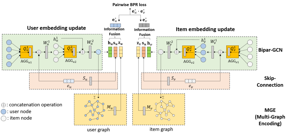
Figure 1: The overall architecture of Multi-GCCF.

II-B Graph-based recommendation

Graphs are a natural tool for representing rich pairwise relationship information in recommendation systems. Early works [18, 19, 20] used label propagation and random walks on the user-item interaction graph to derive similarity scores for user-item pairs. With the emerging field in Graph Neural Networks (GNNs) [21, 22, 23, 24], more recent works have started to apply graph neural networks [25, 12, 11]. Graph Convolutional Matrix Completion (GCMC) [25] treats the recommendation problem as a matrix completion task and employs a graph convolution autoencoder. PinSAGE [12] applies a graph neural network on the item-item graph formed by modeling the similarity between items. Neural Graph Collaborative Filtering (NGCF) [11] processes the bipartite user-item interaction graph to learn user and item embeddings.

III Methodology

In this section, we explain the three key components of our method. First, we develop a Bipartite Graph Convolutional Neural Network (Bipar-GCN) that acts as an encoder to generate user and item embeddings, by processing the user-item interaction bipartite graph. Second, a Multi-Graph Encoding layer (MGE) encodes latent information by constructing and processing multiple graphs: besides the user-item bipartite graph, another two graphs represent user-user similarities and item-item similarities respectively. Third, a skip connection structure between the initial node feature and final embedding allows us to exploit any residual information in the raw feature that has not been captured by the graph processing. The overall framework of Multi-GCCF is depicted in Figure 1.

III-A Bipartite Graph Convolutional Neural Networks

In a recommendation scenario, the user-item interaction can be readily formulated as a bipartite graph with two types of nodes. We apply a Bipartite Graph Convolutional Neural Network (Bipar-GCN) with one side representing user nodes and the other side representing item nodes, as shown in Figure 2. The Bipar-GCN layer consists of two phases: forward sampling and backward aggregating. The forward sampling phase is designed to deal with the long-tailed nature of the degree distributions in the bipartite graph. For example, popular items may attract many interactions from users while other items may attract very few.

After sampling the neighbors from layers $1$ to $K$, Bipar-GCN encodes the user and item nodes by iteratively aggregating $k$-hop neighborhood information via graph convolution. There are initial embeddings $\mathbf{e}_{u}$ and $\mathbf{e}_{v}$ that are learned for each user $u$ and item $v$. These embeddings are learned at the same time as the parameters of the GCNs. If there are informative input features $\mathbf{x}_{u}$ or $\mathbf{x}_{v}$, then the initial embedding can be a function of the features (e.g., the output of an MLP applied to $\mathbf{x}_{u}$). The layer-$k$ embeddings of the target user $u$ can be represented as:

$$\mathbf{h}^{k}_{u}=\sigma\Big{(}\mathbf{W}_{u}^{k}\cdot\textbf{[}\mathbf{h}_{u}^{k-1};\mathbf{h}_{\mathcal{N}(u)}^{k-1}\textbf{]}\Big{)},\hskip 5.69046pt{\mathbf{h}}^{0}_{u}={\mathbf{e}}_{u}\,,$$ (1)

where $\mathbf{e}_{u}$ are the initial user embeddings, $[\,\,;\,]$ represents concatenation, $\sigma(\cdot)$ is the $\mathrm{tanh}$ activation function, $\mathbf{W}_{u}^{k}$ is the layer-$k$ (user) transformation weight matrix shared across all user nodes. $\mathbf{h}_{\mathcal{N}(u)}^{k-1}$ is the learned neighborhood embedding. To achieve permutation invariance in the neighborhood, we apply an element-wise weighted mean aggregator:

$$\mathbf{h}_{\mathcal{N}(u)}^{k-1}=\mathrm{AGGREGATOR_{u}}\Big{(}\left\{\mathbf{h}^{k-1}_{v},v\in\mathcal{N}(u)\right\}\Big{)}\,,$$ (2)

$$\mathrm{AGGREGATOR_{u}}=\sigma\left(\mathrm{MEAN}\left(\left\{\mathbf{h}_{v}^{k-1}\cdot\mathbf{Q}_{u}^{k},v\in\mathcal{N}(u)\right\}\right)\right).$$

Here $\mathbf{Q}_{u}^{k}$ is the layer-$k$ (user) aggregator weight matrix, which is shared across all user nodes at layer $k$, and $\mathrm{MEAN}$ denotes the mean of the vectors in the argument set.

Similarly, the embedding of target item node $v$ can be generated using another set of (item) transformation and aggregator weight matrices:

$$\mathbf{h}^{k}_{v}=\sigma\Big{(}\mathbf{W}_{v}^{k}\cdot\textbf{[}\mathbf{h}_{v}^{k-1};\mathbf{h}_{\mathcal{N}(v)}^{k-1}\textbf{]}\Big{)},\hskip 5.69046pt{\mathbf{h}}^{0}_{v}={\mathbf{e}}_{v}\,,$$

$$\mathbf{h}_{\mathcal{N}(v)}^{k-1}=\mathrm{AGGREGATOR_{v}}\Big{(}\left\{\mathbf{h}^{k-1}_{u},u\in\mathcal{N}(v)\right\}\Big{)}\,,$$ (3)

$$\mathrm{AGGREGATOR_{v}}=\sigma\left(\mathrm{MEAN}\left(\left\{\mathbf{h}_{u}^{k-1}\cdot\mathbf{Q}_{v}^{k},u\in\mathcal{N}(v)\right\}\right)\right)\,.$$

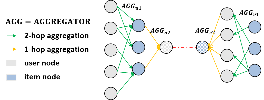
Figure 2: The accumulation of information in the bipartite user-item interaction graph.

III-B Multi-Graph Encoding Layer

To alleviate the data sparsity problem in CF, we propose a Multi-Graph Encoding (MGE) layer, which generates an additional embedding for a target user or item node by constructing two additional graphs and applying graph convolutional learning on them.

In particular, in addition to the user-item bipartite graph, we construct a user-user graph and an item-item graph to capture the proximity information among users and items. This proximity information can make up for the very sparse user-item interaction bipartite graph. The graphs are constructed by computing pairwise cosine similarities on the rows or columns of the rating/click matrix.

In the MGE layer, we generate embeddings for target nodes by aggregating the neighborhood features using a one-hop graph convolution layer and a sum aggregator:

Here $\mathcal{N}^{\prime}(u)$ denotes the one-hop neighbourhood of user $u$ in the user-user graph and $\mathcal{N}^{\prime}(v)$ denotes the one-hop neighbourhood of item $v$ in the item-item graph. $\mathbf{M}_{u}$ and $\mathbf{M}_{v}$ are the learnable user and item aggregation weight matrices, respectively.

In contrast to the Bipar-GCN layer, no additional neighbour sampling is performed in the MGE layer. We select thresholds based on the cosine similarity that lead to an average degree of 10 for each graph.

By merging the outputs of the Bipar-GCN and MGE layers together, we can take advantage of the different dependency relationships encoded by the three graphs. All three graphs can be easily constructed from historical interaction data alone, with very limited additional computation cost.

III-C Skip-connection with Original Node Features

We further refine the embedding with information passed directly from the original node features. The intuition behind this is that both Bipar-GCN and MGE focus on extracting latent information based on relationships. As a result, the impact of the initial node features becomes less dominant. The skip connections allows the architecture to re-emphasize these features.

We pass the original features through a single fully-connected layer to generate skip-connection embeddings.

III-D Information Fusion

The bipartite-GCN, MGE layer and skip connections reveal latent information from three perspectives. It is important to determine how to merge these different embeddings effectively. In this work we investigate three methods to summarize the individual embeddings into a single embedding vector:  element-wise sum,  concatenate, and attention mechanism. The exact operation of these three methods is described in Table I. We experimentally compare them in Section IV.

TABLE I: Comparison of different message fusion methods.

	Formula
Element-wise sum	$\mathbf{e}^{*}_{u}=\mathbf{h}_{u}^{K}+\mathbf{z}_{u}+\mathbf{s}_{u}$
Concatenation	$\mathbf{e}^{*}_{u}=[\mathbf{h}_{u}^{K};\mathbf{z}_{u};\mathbf{s}_{u}]$
Attention	$\mathbf{A}_{u}=Softmax\Big{(}W_{a_{s}}\cdot\sigma\big{(}W_{a_{1}}\cdot\mathbf{h}^{K}_{u}+W_{a_{2}}\cdot\mathbf{z}_{u}+W_{a_{3}}\cdot\mathbf{s}_{u}\big{)}\Big{)}$
	$\mathbf{e}^{*}_{u}=\textbf{\big{[}}\mathbf{h}^{K}_{u};\mathbf{z}_{u};\mathbf{s}_{u}\textbf{\big{]}}\cdot\mathbf{A}_{u}$

III-E Model Training

We adapt our model to allow forward and backward propagation for mini-batches of triplet pairs $\{u,i,j\}$. To be more specific, we select unique user and item nodes $u$ and $v=\{i,j\}$ from mini-batch pairs, then obtain low-dimensional embeddings $\{\mathbf{e}_{u},\mathbf{e}_{i},\mathbf{e}_{j}\}$ after information fusion, with stochastic gradient descent on the widely-used Bayesian Personalized Recommendation (BPR) [26] loss for optimizing recommendation models. The objective function is as follows:

where $\mathcal{O}=\{(u,i,j)|(u,i)\in\mathcal{R^{+}},(u,j)\in\mathcal{R^{-}})\}$ denotes the training batch. $\mathcal{R^{+}}$ indicates observed positive interactions. $\mathcal{R^{-}}$ indicates sampled unobserved negative interactions. $\Theta$ is the model parameter set and $\mathbf{e}^{*}_{u}$, $\mathbf{e}^{*}_{i}$, and $\mathbf{e}^{*}_{j}$ are the learned embeddings. We conduct regularization on both model parameters and generated embeddings to prevent overfitting (regularization coefficients $\lambda$ and $\beta$).

TABLE II: The overall performance comparison. Underline indicates the second best model performance. Asterisks denote scenarios where a Wilcoxon signed rank test indicates a statistically significant difference between the scores of the best and second-best algorithms.

	Gowalla		Amazon-Books		Amazon-CDs		Yelp2018
	Recall@20	NDCG@20	Recall@20	NDCG@20	Recall@20	NDCG@20	Recall@20	NDCG@20
BPRMF	0.1291	0.1878	0.0250	0.0518	0.0865	0.0849	0.0494	0.0662
NeuMF	0.1326	0.1985	0.0253	0.0535	0.0913	0.1043	0.0513	0.0719
GC-MC	0.1395	0.1960	0.0288	0.0551	0.1245	0.1158	0.0597	0.0741
PinSage	0.1380	0.1947	0.0283	0.0545	0.1236	0.1118	0.0612	0.0750
NGCF	0.1547	0.2237	0.0344	0.0630	0.1239	0.1138	0.0581	0.0719
Multi-GCCF ($d$=64)	∗0.1595	∗0.2126	∗0.0363	∗0.0656	∗0.1390	∗0.1271	∗0.0667	∗0.0810
Multi-GCCF ($d$=128)	∗0.1649	∗0.2208	∗0.0391	∗0.0705	∗0.1543	∗0.1350	∗0.0686	∗0.0835

IV Experimental Evaluation

We perform experiments on four real-world datasets to evaluate our model. Further, we conduct extensive ablation studies on each proposed component (Bipar-GCN, MGE and skip connect). We also provide a visualization of the learned representation.

IV-A Datasets and Evaluation Metrics

To evaluate the effectiveness of our method, we conduct extensive experiments on four benchmark datasets: Gowalla, Amazon-Books, Amazon-CDs and Yelp2018 . These datasets are publicly accessible, real-world data with various domains, sizes, and sparsity. For all datasets, we filter out users and items with fewer than 10 interactions. Table III summarizes their statistics.

For all experiments, we evaluate our model and baselines in terms of Recall@k and NDCG@k (we report Recall@20 and NDCG@20). Recall@k indicates the coverage of true (preferred) items as a result of top-$k$ recommendation. NDCG@k (normalized discounted cumulative gain) is a measure of ranking quality.

TABLE III: Statistics of evaluation datasets.

Dataset	#User	#Items	#Interactions	Density
Gowalla	29,858	40,981	1,027,370	0.084%
Yelp2018	45,919	45,538	1,185,065	0.056%
Amazon-Books	52,643	91,599	2,984,108	0.062%
Amazon-CD	43,169	35,648	777,426	0.051%

IV-B Baseline Algorithms

We studied the performance of the following models.
Classical collaborative filtering methods: BPRMF [26]. NeuMF [13]. Graph neural network-based collaborative filtering methods: GC-MC[25]. PinSage [17]. NGCF [11].

Our proposed method: Multi-GCCF, which contains two graph convolution layers on the user-item bipartite graph (2-hop aggregation), and one graph convolution layer on top of both the user-user graph and the item-item graph to model the similarities between user-pairs and item-pairs.

IV-C Parameter Settings

We optimize all models using the Adam optimizer with the xavier initialization. The embedding size is fixed to 64 and the batch size to 1024, for all baseline models. Grid search is applied to choose the learning rate and the coefficient of $L_{2}$ normalization over the ranges {0.0001, 0.001, 0.01, 0.1} and {$10^{-5}$, $10^{-4}$, …, $10^{-1}$}, respectively. As in [11], for GC-MC and NGCF, we also tune the dropout rate and network structure. Pre-training [13] is used in NGCF and GC-MC to improve performance. We implement our Multi-GCCF model in PyTorch and use two Bipar-GCN layers with neighborhood sampling sizes $S_{1}=15$ and $S_{2}=10$. The output dimension of the first layer is fixed to 128; the final output dimension is selected from $\{64,128\}$ for different experiments. We set the input node embedding dimension to $512$. The neighborhood dropout ratio is set to $0.2$. The regularization parameters in the objective function are set to $\lambda=0.01$ and $\beta=0.02$.

IV-D Comparison with Baselines

Table II reports the overall performance compared with baselines. Each result is the average performance from 5 runs with random weight initializations.

We make the following observations:

• Multi-GCCF consistently yields the best performance for all datasets. More precisely, Multi-GCCF improves over the strongest baselines with respect to recall@20 by $9.01$%, $12.19$%, $5.52$%, and $3.10$% for Yelp2018, Amazon-CDs, Amazon-Books and Gowalla, respectively. Multi-GCCF further outperforms the strongest baselines by $12.41$%, $15.43$%, $24.54$% and $6.39$% on recall@20 for Yelp2018, Amazon-CDs, Amazon-Books and Gowalla, respectively, when increasing the latent dimension. For the NDCG@20 metric, Multi-GCCF outperforms the next best method by $5$% to $25$% on three dataset. Further, This suggests that, exploiting the latent information by utilizing multiple graphs and efficiently integrating different embeddings, Multi-GCCF ranks relevant items higher in the recommendation list.

TABLE IV: Ablation studies.

Architecture	Yelp2018
	Recall@20	NDCG@20
Best baseline ($d$=64)	0.0612	0.0744
Best baseline ($d$=128)	0.0527	0.0641
1-hop Bipar-GCN	0.0650	0.0791
2-hop Bipar-GCN	0.0661	0.0804
2-hop Bipar-GCN + skip connect	0.0675	0.0821
2-hop Bipar-GCN + MGE	0.0672	0.0818
Multi-GCCF ($d$=128)	0.0686	0.0835

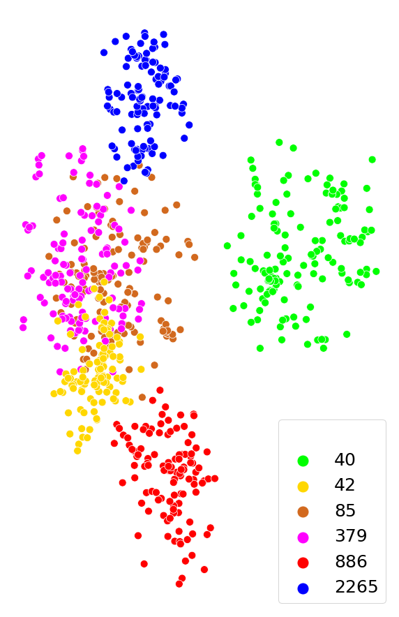
(a) BPRMF

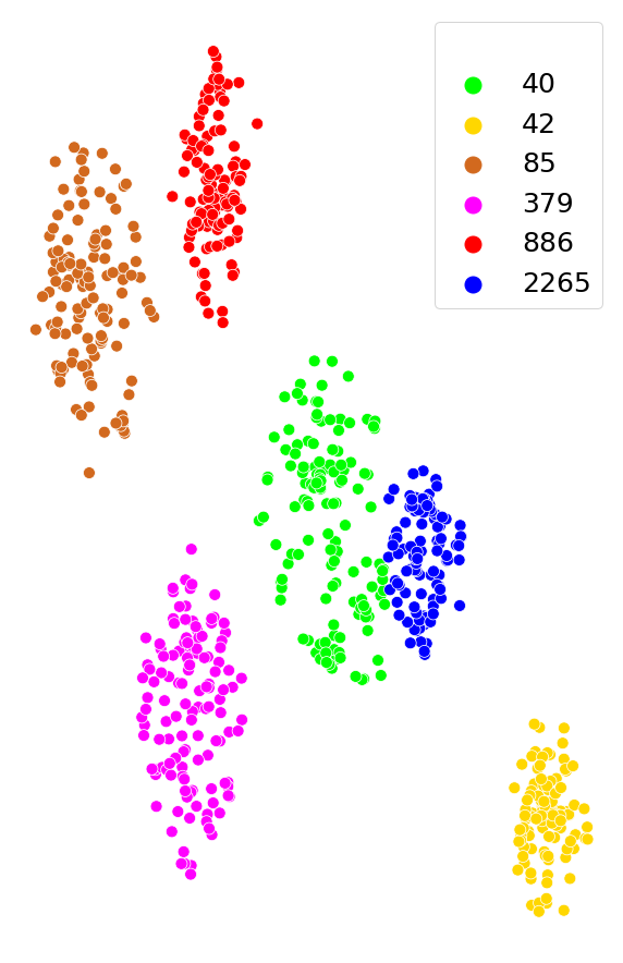
(b) Multi-GCCF

Figure 3: Visualization of the t-SNE transformed representations derived between BPRMF and Multi-GCCF on Amazon-CDs. Numbers in the legend are user IDs.

IV-E Ablation Analysis

To assess and verify the effectiveness of the individual components of our proposed Multi-GCCF model, we conduct an ablation analysis on Gowalla and Yelp2018 in Table IV. The table illustrates the performance contribution of each component. The output embedding size is 128 for all ablation experiments. We compare to $d=64$ baselines because they outperform the $d=128$ versions.

We make the following observations:

• All three main components of our proposed model, Bipar-GCN layer, MGE layer, and skip connection, are demonstrated to be effective.

• Our designed Bipar-GCN can greatly boost the performance with even one graph convolution layer on both the user side and the item side. Increasing the number of graph convolution layers can slightly improve the performance.

• Both MGE layer and skip connections lead to significant performance improvement.

• Combining all three components leads to further improvement, indicating that the different embeddings are effectively capturing different information about users, items, and user-item relationships.

TABLE V: Comparison of different information fusion methods when $d=128$.

	Gowalla		Amazon-CDs
	Recall@20	NDCG@20	Recall@20	NDCG@20
element-wise sum	0.1649	0.2208	0.1543	0.1350
concatenation	0.1575	0.2179	0.1432	0.1253
attention	0.1615	0.2162	0.1426	0.1248

IV-F Effect of Different Information Fusion Methods

As we obtain three embeddings from different perspectives, we compare different methods to summarize them into one vector: element-wise sum, concatenation, and attention. Table V shows the experimental results for Gowalla and Amazon-CDs. We make the following observations: Summation performs much better than concatenation and attention. Summation generates an embedding of the same dimension as the component embeddings and does not involve any additional learnable parameters. The additional flexibility of attention and concatenation may harm the generalization capability of the model.

IV-G Embedding Visualization

Figure 3 provides a visualization of the representations derived from BPRMF and Multi-GCCF. Nodes with the same color represent all the item embeddings from one user’s clicked/visited history, including test items that remain unobserved during training. We find that both BPRMF and our proposed model have the tendency to encode the items that are preferred by the same user close to one another. However, Multi-GCCF generates tighter clusters, achieving a strong grouping effect for items that have been preferred by the same user.

V Conclusion

In this paper we have presented a novel collaborative filtering procedure that incorporates multiple graphs to explicitly represent user-item, user-user and item-item relationships. The proposed model, Multi-GCCF, constructs three embeddings learned from different perspectives on the available data. Extensive experiments on four real-world datasets demonstrate the effectiveness of our approach, and an ablation study quantitatively verifies that each component makes an important contribution. Our proposed Multi-GCCF approach is well supported under the user-friendly and efficient GNN library developed in MindSpore, a unified training and inference Huawei AI framework.

References

- [1] F. Ricci, L. Rokach, B. Shapira, and P. B. Kantor, Recommender Systems Handbook, 1st ed. Berlin, Heidelberg: Springer-Verlag, 2010.
- [2] S. Rendle, “Factorization machines,” in Proc. IEEE Int. Conf. Data Mining, 2010.
- [3] Y. Hu, Y. Koren, and C. Volinsky, “Collaborative filtering for implicit feedback datasets,” in Proc. IEEE Int. Conf. Data Mining, 2008.
- [4] Y. Juan, Y. Zhuang, W. Chin, and C. Lin, “Field-aware factorization machines for CTR prediction,” in Proc. ACM Conf. Recommender Systems, 2016.
- [5] H. Cheng, L. Koc, J. Harmsen et al., “Wide & deep learning for recommender systems,” in Proc. Workshop Deep Learning for Recommender Systems, 2016.
- [6] P. Covington, J. Adams, and E. Sargin, “Deep neural networks for youtube recommendations,” in Proc. ACM Conf. Recommender Systems, 2016.
- [7] J. B. Schafer, D. Frankowski, J. L. Herlocker, and S. Sen, “Collaborative filtering recommender systems,” in The Adaptive Web, Methods and Strategies of Web Personalization, 2007.
- [8] Y. Koren, R. M. Bell, and C. Volinsky, “Matrix factorization techniques for recommender systems,” IEEE Computer, vol. 42, no. 8, pp. 30–37, 2009.
- [9] T. Hofmann, “Latent semantic models for collaborative filtering,” ACM Trans. Inf. Syst., vol. 22, pp. 89–115, 2004.
- [10] Y. Koren, “Factorization meets the neighborhood: a multifaceted collaborative filtering model,” in Proc. ACM SIGKDD Int. Conf. Knowledge Discovery and Data Mining, 2008.
- [11] X. Wang, X. He, M. Wang, F. Feng, and T.-S. Chua, “Neural graph collaborative filtering,” in Proc. ACM Int. Conf. Research and Development in Information Retrieval, 2019.
- [12] R. Ying, R. He, K. Chen, P. Eksombatchai, W. L. Hamilton, and J. Leskovec, “Graph convolutional neural networks for web-scale recommender systems,” in Proc. ACM Int. Conf. Knowledge Discovery & Data Mining, 2018.
- [13] X. He, L. Liao, H. Zhang, L. Nie, X. Hu, and T. Chua, “Neural collaborative filtering,” in Proc. Int. Conf. World Wide Web, 2017.
- [14] B. Liu, R. Tang, Y. Chen, J. Yu, H. Guo, and Y. Zhang, “Feature generation by convolutional neural network for click-through rate prediction,” in Proc. World Wide Web Conference, 2019.
- [15] J. Lian, X. Zhou, F. Zhang, Z. Chen, X. Xie, and G. Sun, “xDeepFM: Combining explicit and implicit feature interactions for recommender systems,” in Proc. ACM SIGKDD Int. Conf. Knowledge Discovery & Data Mining, 2018.
- [16] H. Guo, R. Tang, Y. Ye, Z. Li, and X. He, “Deepfm: A factorization-machine based neural network for CTR prediction,” in Proc. Int. Joint Conf. Artificial Intelligence, 2017.
- [17] Y. Qu, B. Fang, W. Zhang, R. Tang, M. Niu, H. Guo, Y. Yu, and X. He, “Product-based neural networks for user response prediction over multi-field categorical data,” ACM Trans. Inf. Syst., vol. 37, no. 1, pp. 5:1–5:35, 2019.
- [18] M. Gori and A. Pucci, “Itemrank: A random-walk based scoring algorithm for recommender engines,” in Proc. Int. Joint Conf. Artificial Intelligence, Hyderabad, India, 2007.
- [19] X. He, M. Gao, M. Kan, and D. Wang, “Birank: Towards ranking on bipartite graphs,” CoRR, vol. abs/1708.04396, 2017. [Online]. Available: http://arxiv.org/abs/1708.04396
- [20] J. Yang, C. Chen, C. Wang, and M. Tsai, “Hop-rec: high-order proximity for implicit recommendation,” in Proc ACM Conf. Recommender Systems, 2018.
- [21] T. N. Kipf and M. Welling, “Semi-supervised classification with graph convolutional networks,” in Proc. Int. Conf. Learning Representations, 2017.
- [22] W. L. Hamilton, Z. Ying, and J. Leskovec, “Inductive representation learning on large graphs,” in Proc. Adv. Neural Inf. Proc. Systems, 2017.
- [23] Y. Zhang and M. Rabbat, “A graph-CNN for 3D point cloud classification,” in Proc. IEEE Int. Conf. Acoustics, Speech and Signal Processing, 2018.
- [24] Y. Zhang, S. Pal, M. Coates, and D. Üstebay, “Bayesian graph convolutional neural networks for semi-supervised classification,” in Proc. AAAI Int. Conf. Artificial Intelligence, 2019.
- [25] R. van den Berg, T. N. Kipf, and M. Welling, “Graph convolutional matrix completion,” in Proc. ACM SIGKDD Int. Conf. Knowledge Discovery and Data Mining, 2018.
- [26] S. Rendle, C. Freudenthaler, Z. Gantner, and L. Schmidt-Thieme, “BPR: Bayesian personalized ranking from implicit feedback,” in Proc. Conf. Uncertainty in Artificial Intelligence, 2009.