Patterns, localized structures and fronts in a reduced model of clonal plant growth

Abstract

A simplified model of clonal plant growth is formulated, motivated by observations of spatial structures in Posidonia oceanica meadows in the Mediterranean Sea. Two levels of approximation are considered for the scale-dependent feedback terms. Both take into account mortality and clonal, or vegetative, growth as well as competition and facilitation, but the first version is nonlocal in space while the second is local. Study of the two versions of the model in the one-dimensional case reveals that both cases exhibit qualitatively similar behavior (but quantitative differences) and describe the competition between three spatially extended states, the bare soil state, the populated state, and a pattern state, and the associated spatially localized structures. The latter are of two types, holes in the populated state and vegetation patches on bare ground, and are organized within distinct snaking bifurcation diagrams. Fronts between the three extended states are studied and a transition between pushed and pulled fronts identified. Numerical simulations in one spatial dimension are used to determine front speeds and confront the predictions from the marginal stability condition for pulled fronts.

I Introduction

Vegetation distribution in space is often found to be spatially inhomogeneous even in quite homogeneous terrains, a factor that has been recognized as very relevant to understanding ecosystem resilience, functioning and health Meron (2015); Rietkerk et al. (2004); Barbier et al. (2006); Watt (1947). Spatial self-organization of different types of plants has been reported and modeled in a wide range of habitats, from arid or semiarid environments to wetlands Rietkerk et al. (2004); Barbier et al. (2006); Rietkerk and van de Koppel (2008); Meron (2012) and, more recently, in submerged seagrass meadows Ruiz-Reynés et al. (2017). Detailed models of the competition of plants for scarce water have been set up to understand pattern formation in dry ecosystems von Hardenberg et al. (2001); Gilad et al. (2007a, b); Gandhi et al. (2018). In other approaches, water is not explicitly modeled but a generic approach using an integral kernel, which takes into account nonlocal competition processes with typical interaction ranges, is used Lefever and Lejeune (1997); Martínez-García et al. (2013, 2014); Fernandez-Oto et al. (2014); Cisternas et al. (2020). This last approach is more easily generalizable to situations in which water is not the limiting resource driving competitive interactions, as in the case of marine plants Ruiz-Reynés et al. (2017).

In most of the previous models, propagation of vegetation over a landscape is assumed to occur by seed dispersal, modeled as an isotropic diffusion. Clonal growth by rhizome elongation, however, has directional characteristics, a fact that has been modeled at various levels of detail Ruiz-Reynés et al. (2017); Ruiz-Reynés and Gomila (2019); Ruiz-Reynés et al. (2020). In Ruiz-Reynés et al. (2017) the so-called advection-branching-death (ABD) model, describing the growth of clonal plants at a landscape level, was introduced. This model consists of two partial integro-differential equations for the evolution of the density of shoots and apices of the plant. This model was derived directly from the microscopic mechanisms involved in clonal plant growth, namely rhizome elongation (which appears in the model as an advection term), branching, and death, and its parameters can be directly linked to rates and quantities directly measured in underwater seagrass meadows Ruiz-Reynés et al. (2017). Plant interactions were modeled in terms of a nonlocal competition kernel. Although the model describes vegetation distribution in two-dimensional space, the need to include the direction of growth of the apices introduces a new (angular) variable that makes this model effectively three-dimensional and so carries a high computational cost. Fortunately, this angular coordinate does not appear to play a crucial role in most of the observed phenomenology Ruiz-Reynés and Gomila (2019). For this reason, in Ruiz-Reynés et al. (2020) a single equation for the total density of shoots that captures all the dynamical regimes of the ABD model was proposed, the clonal-growth model. Under certain approximations this equation can be derived from the full model, establishing a connection between the effective parameters of the simple description and the biologically relevant parameters of the full model.

Vegetation patterns can be extended, in the sense that the same type of biomass organization extends over a large area (for example, homogeneous or periodic distributions) or localized. Examples of the later are a patch or several patches of vegetation surrounded by bare soil, or a bare gap or set of gaps on an otherwise vegetated area. Different extended states can occur in different regions of a landscape, giving rise to fronts between them where they meet. Such fronts can remain static or move, describing the invasion of one type of biomass configuration by another or its retreat. In this work we study in detail the spatially extended, localized, and front solutions of two versions of the clonal-growth model Ruiz-Reynés et al. (2020), obtained by keeping the nonlocal character of the interactions or replacing them by an effective local description. In contrast to Ruiz-Reynés et al. (2020) we restrict the present study to one spatial dimension, which allows a more detailed analysis and comparison between the two levels of approximation.

The models considered are described in Sec. II. The stationary solutions of the resulting equations are presented and compared in Sec. III. The dynamics of fronts between different states, both stable and unstable, are analyzed in Sec. IV and in some cases the predicted front speeds are compared with those determined via direct numerical simulation.

II Model

In Ref. Ruiz-Reynés et al. (2020) we proposed a sequence of approximations that lead from the full ABD model to a single differential equation describing the evolution of the shoot density of a plant undergoing vegetative or clonal growth, the clonal-growth model. In one spatial dimension, the model reads:

$$\partial_{t}n=(\omega_{b}-\omega_{d}[n])n+d_{0}\partial_{x}^{2}n+d_{1}n\partial_{x}^{2}n+d_{1}\left|\partial_{x}n\right|^{2},$$ (1)

where $n(x,t)$ is the plant shoot density, $\omega_{b}>0$ is the branching rate of the plant, i.e., the birth term, and $\omega_{d}[n]>0$ is the mortality rate, which depends on the density. The terms involving derivatives with coefficients $d_{0}$ and $d_{1}$ arise from rhizome elongation and branching in the original model, and implement the peculiarities of clonal growth. These coefficients may depend on environmental conditions and hence on space, but we take both to be constant. Note that the same coefficient $d_{1}$ appears in the last two terms.

II.1 Version I: full nonlocal interaction

As a first level of description, hereafter version I, we take Eq. (1) and retain the original nonlocal terms accounting for the interaction between plants Ruiz-Reynés et al. (2017):

$$\omega_{d}[n]=\omega_{d0}+\int\int\mathcal{K}(\vec{r}-\vec{r}^{\prime})(1-e^{-an(\vec{r}^{\prime})})d\vec{r}^{\prime}+bn^{2}.$$ (2)

The first term $\omega_{d0}$ in (2) is the intrinsic mortality (mortality in the absence of other plants). The second term accounts for interactions across space in such a way that the density of shoots at a given position can affect the growth in a neighborhood weighted by the kernel $\mathcal{K}(\vec{r}-\vec{r}^{\prime})$. To better control the growth of the solutions and prevent potential blow-up, we also incorporate a local nonlinear term $bn^{2}$, where the parameter $b$ determines the maximum value of the density even in cases where nonlinear effects in the integral kernel might be destabilizing. From the biological point of view this term models local mechanisms of competition (at the level of single shoots, for example) which are different from the non-local ones modeled by the integral kernel.

The kernel $\mathcal{K}$ is taken to be the difference of two normalized Gaussian functions $\mathcal{G}$, both with zero mean but with different magnitudes ($\kappa$, $\mu>0$) and widths ($\sigma_{\kappa}$, $\sigma_{0}$):

$$\mathcal{K}(\vec{r})=\kappa\mathcal{G}(\sigma_{\kappa},\vec{r})-\mu\mathcal{G}(\sigma_{0},\vec{r}).$$ (3)

The first term on the rhs of (3) accounts for all the competitive effects, since it increases the mortality rate, while the second accounts for facilitative effects. Facilitation is taken here to reduce the external factors increasing mortality only; the term $\omega_{d0}$, which is independent of density, encodes these external effects. Hence, the integrated facilitation needs to satisfy $\mu\leq\omega_{d0}$ to ensure positive mortality and avoid unrealistic creation of plants by this term. Here we choose $\mu=\omega_{d0}$ for simplicity. The range of the competitive and facilitative interaction is given by $\sigma_{\kappa}$ and $\sigma_{0}$, respectively. We assume that $\sigma_{k}>\sigma_{0}$, as appropriate for the observations in marine plants Ruiz-Reynés et al. (2017).

The location in parameter space of the different spatially uniform states of this version of the reduced model is summarized in Fig. 1 together with their stability properties and is the same in both one and two dimensions. In addition to qualitative agreement with the dynamical regimes of the full ABD model Ruiz-Reynés et al. (2017), version I of the reduced model reproduces to a high degree of accuracy the position in parameter space of the modulational instability (MI) of the homogeneously populated solution. This description thus provides quantitatively accurate results, while providing a simplified model of clonal plant growth.

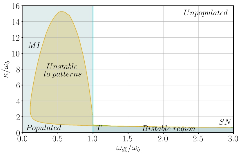
Figure 1: Phase diagram for version I of the model. The regions where the populated (P) and unpopulated (U) states are stable are shown in bright blue and white, respectively, while the coexistence region between these two states is shown in darker blue. The region where P is unstable to patterns is shown in yellow. The symbol $T$ refers to a transcritical bifurcation at $\omega_{d0}/\omega_{b}=1$, while $SN$ refers to a saddle-node bifurcation where P undergoes a fold. The curve labeled $MI$ corresponds to the onset of modulational (or Turing) instability that is responsible for the appearance of spatial patterns in the model. The parameters are $\omega_{b}=0.06$ $year^{-1}$, $b=1.25$ $cm^{4}year^{-1}$, $\sigma_{\kappa}=$ $2851.4$ $cm$, $a=27.38$ $cm^{2}$, $\sigma_{0}=203.7$ $cm$, $d_{0}=631.2$ $cm^{2}year^{-1}$, $d_{1}=4842.1$ $cm^{4}year^{-1}$. These parameters are appropriate for the marine plant Posidonia oceanica Ruiz-Reynés et al. (2017, 2020).

II.2 Version II: effective local description

A second level of approximation, version II, results from performing a moment expansion of the integral term $\omega_{d}[n]$ and truncating at the lowest possible order. Specifically, we first expand the exponential inside the integral and then truncate the moment expansion of the kernel at fourth order. The approximation yields qualitative agreement with the behavior of version I (and thus of the ABD model in Ruiz-Reynés et al. (2017)) in terms of the observed dynamical regimes (compare Fig. 2 with Fig. 1). In particular, the general ordering of the different phases in parameter space and the nature of the bifurcations (saddle-node, transcritical, and the MI) bounding them is the same. But there is lack quantitative agreement. The inclusion of higher order terms in the expansion may improve accuracy but implies loss of simplicity. We therefore choose the parameters in version II to preserve as much as possible the behavior of version I while keeping its simple form. The mortality now reads

$$\omega_{d}(n)=\omega_{d0}+a^{\prime}(\kappa-\omega_{b})n+b^{\prime}n^{2}-\alpha\partial_{x}^{2}n-\beta\partial_{x}^{4}n,$$ (4)

with the intrinsic mortality $\omega_{d0}$ the same as before. The second coefficient $a^{\prime}(\kappa-\omega_{b})$ controls the degree of bistability. We write this coefficient in this way to facilitate a comparison with version I. The coefficient $b^{\prime}$ determines the saturation level, while $\alpha$ and $\beta$ come from the expansion of the nonlocal term and are responsible for the presence or absence of spatial patterns. The parameters $a^{\prime}$ and $b^{\prime}$ are chosen to generate a bifurcation diagram similar to that of version I. The conditions imposed are: (i) having the same density of shoots at $\omega_{d0}=\omega_{b}$ and (ii) having the saddle-node bifurcation of the homogeneous populated state at the same value of the mortality rate $\omega_{d0}$. These conditions are imposed at the value $\kappa=0.048year^{-1}$ which will be used throughout the paper. The parameters $\alpha$ and $\beta$ are chosen to generate the modulational or Turing instability at a similar mortality rate as in version I for the same chosen value of $\kappa$, and with a similar critical wavelength.

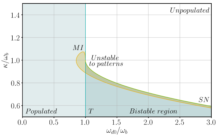
Figure 2: Phase diagram for version II of the model. The color code is as in Fig. 1. The parameters are $\omega_{b}=0.06$ $year^{-1}$, $b^{\prime}=12.5$ $cm^{4}year^{-1}$, $a^{\prime}=100.41$ $cm^{2}year^{-1}$, $\kappa=0.048$ $year^{-1}$, $\alpha=-8.642\cdot 10^{7}$ $cm^{6}year^{-1}$, $\beta=-3.585\cdot 10^{13}$ $cm^{8}year^{-1}$, $d_{0}=508.1$ $cm^{2}year^{-1}$, $d_{1}=6560.6$ $cm^{4}year^{-1}$.

The equation for this version II of the model, resulting from combining Eqs. (1) and (4), was originally derived in Ruiz-Reynés et al. (2020), and some of its properties studied in two dimensions. It has several terms in common with previously studied models. In particular the effect of the nonvariational terms $\left|\partial_{x}n\right|^{2}$ and $n\partial_{x}^{2}n$ on front motion was considered in Alvarez-Socorro et al. (2017) in a model of an optical system. In the context of vegetation patterns, the model discussed in Fernandez-Oto et al. (2019); Parra-Rivas and Fernandez-Oto (2020) is very similar to our version II, although it misses the $\left|\partial_{x}n\right|^{2}$ term, which is characteristic of clonal growth.

III Stationary patterns and localized structures

In this section we discuss the different stationary solutions supported by versions I and II of the model in one dimension. We first show the results for version I with the full nonlocal interaction term, and then for version II based on the truncated moment expansion, highlighting the main differences between them. Throughout we use the mortality rate $\omega_{d0}$ as the main control parameter. In order to follow stationary solutions we use a pseudo-arclength continuation method Keller (1986); Mittelmann (1986) where the Jacobian is calculated in Fourier space. Starting with an initial condition obtained using numerical simulations we continue the stable and unstable branches changing $\omega_{d0}$ as a control parameter.

III.1 Version I: patterns and localized structures

Different solutions are observed when the mortality $\omega_{d0}$ changes as summarized in the bifurcation diagram shown in Fig. 3. When mortality is large the branching rate $\omega_{b}$ is insufficient to sustain growth and the only stable solution is bare soil, the unpopulated state (U). In contrast, when the death rate is small compared to the branching rate the homogeneous populated state (P) prevails. In between one finds a region of coexistence between P and U; this region terminates in a saddle-node bifurcation labeled $SN$. Both the populated and unpopulated states are shown in red in the figure. When the branching and mortality rates are comparable the upper P state may become unstable to spatial modulations that develop into a periodic pattern that we call a stripe pattern (S), shown in green in Fig. 3. The emerging stripe pattern bifurcates subcritically but undergoes a fold, thereby generating a region of coexistence between stable stripes and the stable upper P state for mortalities below MI. The stripe pattern turns out to be rather robust and stable stripes are found far beyond the region of existence of the homogeneous state, coexisting with the bare soil state U over a broad range of values of $\omega_{d0}$ above the transcritical bifurcation $T$ of U. With increasing mortality rate the stable stripes eventually terminate in a fold bifurcation. The unstable S states that result in turn terminate at a second MI or Turing bifurcation located on the unstable (middle) branch of P, very close to zero density (Fig. 3b). We mention that between these two Turing bifurcations there are other pairs of Turing bifurcations that also give rise to spatially periodic stripes but with wavelengths different (smaller and larger) from the critical wavelength corresponding to the MI of the P state, which is the one displayed here. Thus, the S state is by no means unique.

Figure 3 shows that in addition to the S branch, the MI or Turing bifurcation on the upper P branch generates a pair of branches of spatially localized structures (LS) that also emerge subcritically, creating a window in the mortality rate, called a snaking region Woods and Champneys (1999); Coullet et al. (2000); Burke and Knobloch (2006), within which one finds stable stationary states consisting of segments of the periodic S state of arbitrarily large length, embedded in the background P state. The purple lines in Figs. 3 and 4 show the resulting snaking bifurcation diagram revealing the presence of two intertwined LS branches consisting of states with odd and even numbers of close-packed troughs. A single-trough state corresponds to a single region of nearly bare soil embedded in P, i.e., a hole in an otherwise homogeneous state, analogous to fairy circles in two spatial dimensions. Based on the general theory developed for the prototypical Swift-Hohenberg equation we expect that opposing folds on the odd and even branches are connected by (unstable) branches of asymmetric states. Owing to the nonvariational structure of the present problem we expect that these states drift, cf. Mercader et al. (2013). In this work we do not follow unstable states of this type. We also note that the region of existence of LS extends beyond the left fold of the S branch shown in the figure. This is possible when the wavenumber selected by the LS in the snaking region differs sufficiently from the critical wavenumber at MI to force the LS branches to terminate on a different S branch (see Fig. 4). In the present case the resulting snaking region extends almost to the fold of this second S branch indicating that the chosen parameter values are very close to a transition that breaks up the snaking scenario. This transition occurs when the left LS folds touch the left fold of the corresponding pattern state Champneys et al. (2012).

For mortalities larger than the branching rate, $\omega_{d0}>\omega_{b}$, a different type of stable spatially localized structure is found, consisting of isolated vegetation patches on bare soil (see orange lines in Figs. 3 and 5). The bifurcation structure of these LS differs from the previous case, and they do not lie on a standard snaking branch. Instead these states bifurcate from the unstable P branch close to zero density and below the MI bifurcation at which the S state terminates (see inset in Fig. 5). This bifurcation corresponds to a long wavelength instability, and generates a state with wavelength equal to the system size. The low-amplitude one-patch solution that arises is unstable and grows in amplitude with increasing mortality until it reaches a fold where it acquires stability and becomes a high amplitude stable single patch solution. Beyond the fold the patch state continues to grow in amplitude but now for decreasing mortality until it reaches a second fold. Near this second fold the solution starts to change shape, the central part of the patch developing a relative minimum that continues to decrease along the subsequent branch. Thus, the patch starts to divide into two patches until, after a third fold, two low-amplitude LS are present and these gradually decrease in amplitude with decreasing mortality until the branch terminates back on the unstable P branch. Very close to this bifurcation both peaks become very shallow and their maxima move rapidly apart until they are separated by $L/2$, i.e., half the system size. Thus, the termination point corresponds to a pattern-forming bifurcation of the unstable P state to a two-peak state much like the long-wave bifurcation to the single peak state that occurs at a lower value of the density. The bifurcation to the two-peak state is in fact a pitchfork bifurcation, one fork of which corresponds to the termination of the two-peak state generated from the single peak state via peak-splitting as just described, while the other takes part in a similar scenario but based on a two-peak state. This scenario results, again via peak-splitting, in a four-peak state that terminates on P at yet higher (but still small) density (Fig. 5). Once again, close to this termination point the four peaks become equidistant, i.e., separated by $L/4$, allowing this branch to terminate in a pattern-forming bifurcation from a periodic state. In fact this behavior is observed for any number of equispaced identical peaks, even or odd, generated in corresponding bifurcations along the unstable P branch. Similar bifurcation structures have been found in other systems Yochelis et al. (2008); Parra-Rivas et al. (2018a). We conjecture that in the limit of an infinite domain the wavelength along the unstable S branch increases by wavelength doubling that occurs via the same process as that occurring for the one-peak and two-peak states, i.e., via repeated peak-splitting Yochelis et al. (2008); Parra-Rivas et al. (2018a), ultimately reaching the transcritical bifurcation T and zero wavenumber, much as occurs in the Gray-Scott model Doelman et al. (1998, 2012). This scenario is supported by the fact that in all cases the folds on the right align at $\omega_{d0}/\omega_{b}\approx 3.538$, a value that is close to that of the fold on the S branch, while the folds on the left align at $\omega_{d0}/\omega_{b}\approx 2.207$; the intermediate folds are also aligned (at $\omega_{d0}/\omega_{b}\approx 3.044$). Ref. Zelnik et al. (2018) describes a scenario whereby the single peak state may reconnect with or turn into a pattern state.

The stationary solutions shown have been computed using different discretizations $\Delta x$. Periodic solutions have been computed using a domain size equal to one wavelength and have been represented showing multiple wavelengths to emphasize the extended nature of the pattern. For the stripes with critical wavenumber shown in Figs. 3, 4 and 5, the number of grid points is $N=128$ and $\Delta x=0.533$ $m$. For stripes with wavelength selected by the localized structure shown in Figs. 4 $N=128$ and $\Delta x=0.703$ $m$. For all LS $N=1024$. Those with odd and even number of holes shown in Figs. 3 and 4 use $\Delta x=0.615$ $m$ and $\Delta x=0.703$ $m$, respectively. For patches shown in Figs. 3 and 5, $\Delta x=0.509$ $m$.

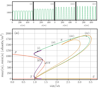
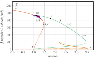
Figure 3: Bifurcation diagram for version I of the model as a function of the ratio $\omega_{d0}/\omega_{b}$. Panel (a) shows the maximum and minimum values of the density $n$ corresponding to the different stationary states while (b) shows the average density. Continuous (dashed) lines represent stable (unstable) solutions. The P and U states are shown in red, while the spatially periodic stripe state S is shown in green (sample S states are shown in the panels above (a)). Spatially localized states (LS) corresponding to holes embedded in the P state are shown in purple while the orange curves show localized structures consisting of patches of vegetation on bare soil, i.e., embedded in the U state. Here $\kappa=0.048$ $year^{-1}$ and the remaining parameters are as in Fig. 1.

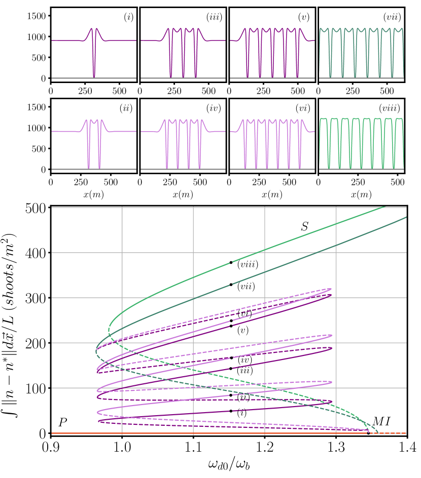
Figure 4: Close-up of the snaking region of version I of the model, emerging from the modulational instability of the P state in Fig. 3 using the norm of the difference between this state and P to reveal details of the snaking bifurcation diagram. The dark purple curve represents LS with an odd number of holes, while the bright purple curve represents LS with an even number. The green curves correspond to stripe patterns S with two different wavenumbers, one with the critical wavenumber and the other with the wavenumber selected by a stationary front between the homogeneous and pattern states, which determines the wavelength within the LS. The upper panels show the solution profiles corresponding to the labeled locations in the bifurcation diagram (lower panel). The parameters are as in Fig. 3.

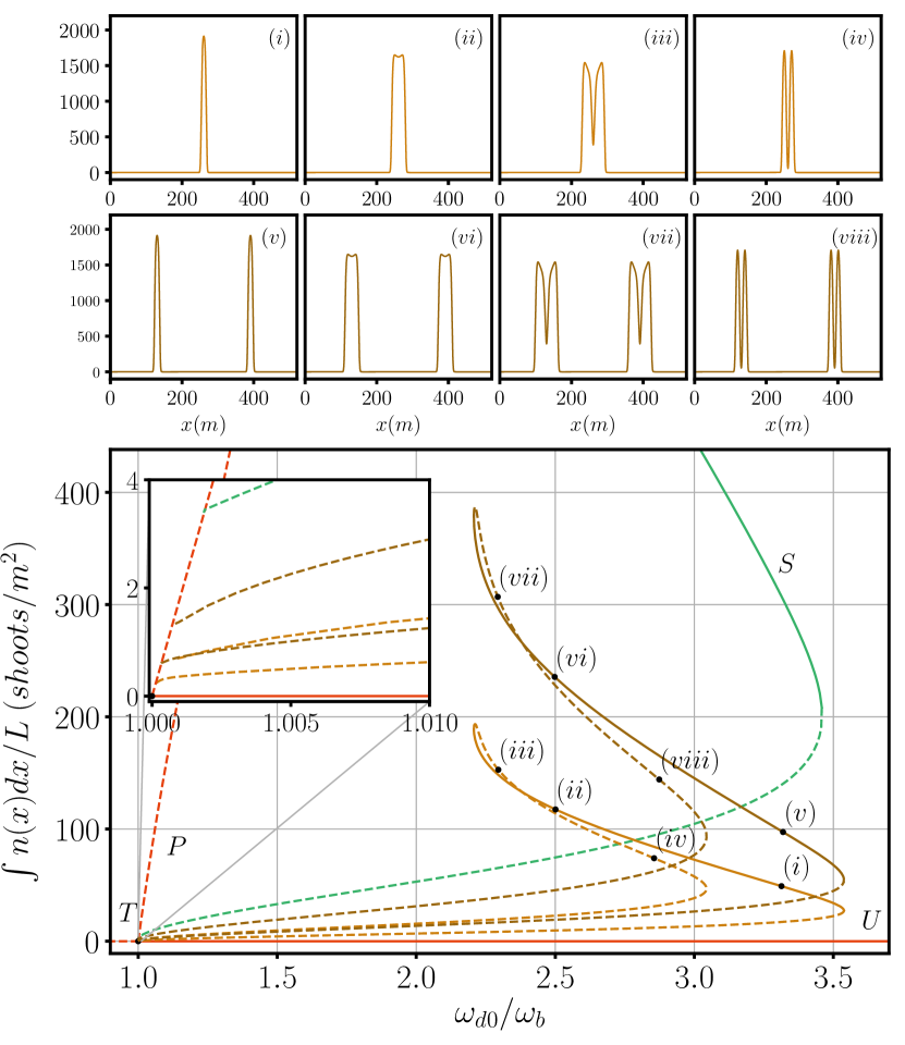
Figure 5: Close-up of the region of vegetation spots on bare soil from version I of the model. Light orange curve represents LS with one peak, while dark orange represents LS with two peaks separated by half the system size. The stripe pattern S with the critical wavenumber is shown in green. The upper panel shows the solution profiles corresponding to the labeled locations in the bifurcation diagram (lower panel). The parameters are as in Fig. 3.

III.2 Version II: patterns and localized structures

Figure 6 shows the corresponding bifurcation diagram for the P, U, S and LS states in version II of the model. The bifurcation scenario is qualitatively similar to that observed in version I (compare Fig. 6 with Fig. 3), confirming the fact that this simpler version of the model captures all the basic mechanisms. However, substantial quantitative differences are observed. For instance, the mortality ranges in which each solution exists are reduced, while the solution profile becomes more triangular. As a result the bare soil minima in the S state are much narrower.

These solutions have been computed following the same procedure as for version I of the model. For the stripes $N=128$, while for all localized structures $N=2048$, with $\Delta x=0.448$ $m$ in all cases.

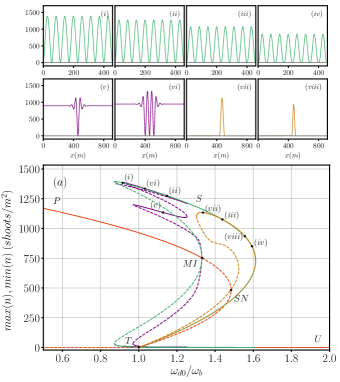
Figure 6: Bifurcation diagram and sample stationary solutions of version II as a function of the ratio $\omega_{d0}/\omega_{b}$. The color scheme, labels and line types are as in Fig. 3; $\kappa=0.048$ $year^{-1}$ and the remaining parameters are as in Fig. 2.

IV Fronts

Figure 3 for version I and Fig. 6 for version II reveal the existence of several different regions of coexistence between the U, P and S states owing to the presence of multiple stable solutions, raising the possibility of a number of different fronts connecting these states. As many as three stable spatially extended states can coexist simultaneously, a situation that also arises in other vegetation pattern-forming models Zelnik et al. (2018). Here we study the fronts connecting the populated state with the unpopulated state (P-U fronts), the stripe pattern with the populated state (S-P fronts) and the stripe pattern with the unpopulated state (S-U fronts). We note that our one-dimensional study is also relevant for flat fronts in two dimensions advancing in the normal direction.

However, flat fronts may experience transversal instabilities in two dimensions changing the front profile (see e.g. Fernandez-Oto et al. (2019)). From this perspective, a dedicated investigation is needed to achieve a complete description of front propagation in two dimensions. Nevertheless, the propagation of fronts is strongly influenced by the stability range of LS, where the one- and two-dimensional cases show general agreement Ruiz-Reynés et al. (2020).

Front dynamics depend strongly on the stability of the states that are involved. The speed of moving fronts connecting two linearly stable states necessarily depends on nonlinear processes, i.e. processes occurring beyond the immediate vicinity of the front. Such fronts are called pushed van Saarloos (2003). In contrast, fronts of constant form describing the invasion of a linearly unstable state by a stable one may travel with a speed determined via a linear mechanism that requires that perturbations ahead of the front grow at just such a rate that a front of constant form is maintained van Saarloos (2003). These fronts are thus pulled by the linear instability ahead of them. It should be mentioned, however, that the existence of pulled fronts does not imply that such fronts are selected. Pushed fronts can exist in the same parameter regime and these would travel with a different speed. In the case of coexistence between pulled and pushed fronts, the front with the larger velocity is usually the one that is observed Hari and Nepomnyashchy (2000); Archer et al. (2014).

The speed $v$ of a pulled front can be obtained by considering infinitesimal perturbations, of the form $e^{ikx+\lambda\left(k\right)t}$ or equivalently $e^{ikx^{\prime}+\Lambda(k)t}$ with $\Lambda(k)=ikv+\lambda(k)$, to the unstable state in the comoving reference frame $x^{\prime}=x-vt$ van Saarloos (2003); van Saarloos and Hohenberg (1992). Applying the condition of marginal stability, i.e., that in the frame moving at speed $v$ perturbations neither grow nor decay, leads to the requirement that the (complex) group speed and the growth rate of the perturbation both vanish, yielding three conditions that are solved for the unknown speed $v$ of the front and the real and imaginary wavenumbers at the leading edge of the front. Specifically, the conditions are $\textrm{Re}\left[\Lambda(k)\right]$=0 and $d\Lambda(k)/dk=0$, where $k=k_{r}+ik_{i}$, the real and imaginary parts of $k$ representing the wavenumber ahead of the front and the spatial decay of its envelope. These equations can be written as $v=\textrm{Re}\left[\lambda(k)\right]/k_{i}$, $\textrm{Re}\left[d\lambda(k)/dk\right]=0$ and $v=-\textrm{Im}\left[d\lambda(k)/dk\right]$. This calculation is further developed in the Appendix, and applied to specific fronts in our model systems as described in the following sections.

IV.1 Fronts in version I of the model

In this section we show the results obtained with version I, using the bare mortality $\omega_{d0}$ as the main control parameter and keeping the other parameters as in Fig. 3. Our numerical simulations use a pseudospectral method with periodic boundary conditions and $\Delta t=1.667\cdot 10^{-3}$ $years$, $\Delta x=0.255$ $m$ and $N=4096$, $8192$ and $16384$ grid points starting with a homogeneous initial condition, the U or P state, with a very narrow step function at $x=0$ to excite a competing solution. In the cases in which two distinct fronts are possible (tristability) we use the profile of the desired front obtained for other values of the mortality as initial condition.

We study first the P-U fronts between the two homogeneous solutions. We can distinguish two cases. When $\omega_{d0}/\omega_{b}>1$ (but below a value at which the state P behind the front destabilizes, see below) the front is a pushed front as both P and U are stable. The front speed as well as the direction of advance is thus determined by nonlinearities. We observe numerically that P always invades U. Figure 7 shows an example of this type of front. On general grounds, one would expect to find a sufficiently large value of the mortality, a Maxwell point, beyond which the direction of the front reverses and the bare soil invades the populated solution. However, it turns out that this occurs beyond the mortality rate for the instability of the P solution to pattern formation (MI), and we never observe this type of desertification front.

For $\omega_{d0}/\omega_{b}<1$ the U state is unstable and a pulled front whereby P advances into U exists. Its speed can be computed from the marginal stability approach. In Fig. 8 we show, as a function of $\omega_{d0}/\omega_{b}$, the speed $v$ of the pulled front computed analytically (red line, see Appendix) and from numerical simulations (red dots). It is clear that the marginal stability prediction of the speed fails. The front speed for $\omega_{d0}/\omega_{b}<1$ appears to be a continuation of the pushed front speed for $\omega_{d0}/\omega_{b}>1$. We have investigated the discrepancy between the linear marginal stability prediction and numerics by performing numerical simulations in which the nonlinear terms that do not appear in the linear calculation are removed. First we removed the term $d_{1}\left|\partial_{x}n\right|^{2}$ but the resulting change in the speed of the front is small (blue dot in Fig. 8 for $\omega_{d0}/\omega_{b}=0.4$). We then removed the nonlocal competition term as well by setting $\sigma_{\kappa}=0$ (black dot in Fig. 8). In this second case the velocity changes dramatically and coincides with the linear marginal stability prediction. This result points to the nonlocal interaction term as the source of discrepancy between the linear marginal stability prediction and the speed of the front in the full system. We ascribe this effect to an inhibiting effect of existing plants at the edge of the front on the growth of plants a certain distance ahead of the front, thereby decreasing the speed of propagation. This interpretation is supported by the presence of a density maximum in the front profile located at the front edge and generated by long range interactions (Fig. 7). We note that in systems of reaction-diffusion equations the speed selection problem is more complex (the fastest front is not always the one selected) than in single species problems and nonlocal systems such as that studied here are, somewhat loosely, equivalent to a higher-dimensional system Holzer and Scheel (2014). Other effects of nonlocal terms on the speed of fronts have been studied in Gelens et al. (2010); Fernandez-Oto et al. (2013, 2014).

The P-U front is observed for $\omega_{d0}/\omega_{b}$ below a critical value $1.325\pm 0.008$ (which is close to but below the MI occurring at $\omega_{d0}/\omega_{b}\approx 1.345$). In this region P always invades U and no Maxwell point (i.e., a value of $\omega_{d0}$ at which propagation direction reverses) is found. When $\omega_{d0}/\omega_{b}\gtrsim 1.325\pm 0.008$, the P state behind the front destabilizes so that the front generates a stripe pattern in its wake, i.e., it becomes a S-U front. We note, however, that there is a small region ($1.277\pm 0.014\lesssim\omega_{d0}/\omega_{b}\lesssim 1.325\pm 0.008$) of coexistence between the two fronts (yellow dots in Fig. 8).

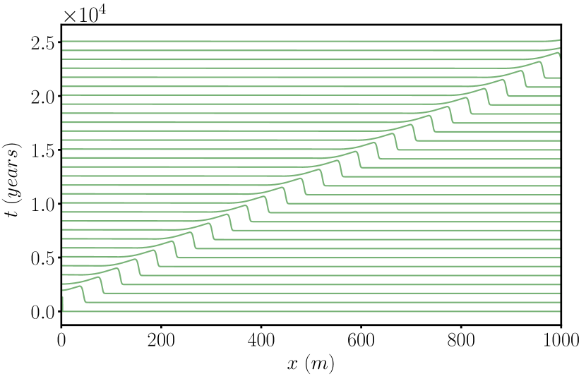
Figure 7: Space-time representation of a pushed P-U front whereby a stable P state invades a stable U state in version I of the model. The figure shows $n(x,t)$ along the vertical axis at successive times $t$, displaced in the vertical by $t$. The front travels with speed $v\approx$ $0.044$ $m/year$. Here $\omega_{d0}=0.0679$ $year^{-1}$ ($\omega_{d0}/\omega_{b}=1.132$) and the remaining parameters are as in Fig. 3.

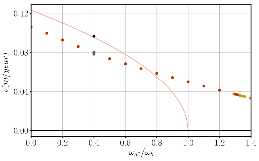
Figure 8: Speed $v$ of the P-U (red dots) and S-U (yellow dots) fronts in version I of the model as a function of $\omega_{d0}/\omega_{b}$. Solid line represents the linear marginal stability prediction for a pulled P-U front. The blue dot corresponds to a numerical simulation without the term $\left|\partial_{x}n\right|^{2}$, while the black dot corresponds to removing in addition all nonlocal competition ($\sigma_{\kappa}=0$). Parameters are as in Fig. 3.

Figure 9 shows a space-time representation of an S-U front at $\omega_{d0}/\omega_{b}=1.395$. This front, whereby S invades U, is pushed since both S and U are stable at this mortality rate. The front’s leading edge is very steep, and is followed by a sloping plateau that leads to the formation of a deep hole that is characteristic of the S state at this mortality rate. Once the hole forms the plateau relaxes, reproducing the S profile near its maxima. Note that in the reference frame moving with the front the deposition of successive holes is an oscillatory process with a well-defined temporal period and we conjecture that, in that reference frame, the S-U front forms via a (subcritical) Hopf bifurcation of the P-U front. For this reason the leading edge of the S-U front at, say, $\omega_{d0}/\omega_{b}\sim 1.395$ closely resembles that of the corresponding P-U front (Fig. 10), a fact that is likely responsible for the similar speeds of these two fronts (Figs. 8 and 11). Indeed, Figs. 10(a,c) show the profiles of the S-U and P-U fronts at equispaced times, with (a) showing the initiation of the deep hole associated with the S state. No such hole is generated behind a P-U front. Panels (b,d) show that these fronts can be viewed, respectively, as heteroclinic connections between a limit cycle (the S state) and the trivial or zero state (the U state), and between two equilibria, one corresponding to the P state and the other to the U state, indicated by the black spots in the figure. Note the similarity of the trajectory leaving the zero state. In both cases the density profile has a pronounced maximum just behind the leading edge of the front, which we ascribe to the absence of competition ahead of the front. Such overshoots are characteristic of fairy circles in arid ecosystems as well.

The S-U front is observed for $\omega_{d0}/\omega_{b}\gtrsim 1.277\pm 0.014$ and travels with a speed that decreases monotonically with $\omega_{d0}$ until $\omega_{d0}/\omega_{b}\approx 2.205\pm 0.005$ where its speed vanishes (Fig. 11). In this interval of mortalities the S-U front selects a well-defined and nonzero wavenumber $q$ in its wake, with values shown in Fig. 11. Beyond $\omega_{d0}/\omega_{b}\approx 2.205$ no new holes are generated and a stationary state consisting of equispaced, widely separated stripes is observed. The stopping of the front is not the result of conventional front pinning Coullet et al. (2000), since the spatial eigenvalues of U cannot be complex owing to the requirement that the density $n(x)$ is everywhere non-negative. We have been unable to determine whether the selected wavenumber $q$ remains nonzero at $\omega_{d0}/\omega_{b}\approx 2.205$ but we mention that the region $\omega_{d0}/\omega_{b}\gtrsim 2.205$ is in any case populated by a number of stable stationary equispaced-patch states resembling the 1-peak, 2-peak localized structures described in Sec. III.1; only one of these would be selected by the moving front as $\omega_{d0}/\omega_{b}\to 2.205$, most likely corresponding to $q=2\pi/L$ or the 1-peak state. Thus, the transition at $\omega_{d0}/\omega_{b}\approx 2.205$ would correspond to a transition from a state with an intrinsic wavelength $2\pi/q$ to one where the wavelength is determined by the domain size $L$.

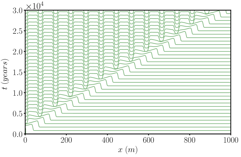
Figure 9: Space-time representation of a pushed S-U front connecting a stable stripe pattern S with the unpopulated state U in version I of the model. The front travels with speed $v\approx 0.033$ $m/year$; $\omega_{d0}=0.0837$ $year^{-1}$ ($\omega_{d0}/\omega_{b}=1.395$) and the remaining parameters are as in Fig. 3.

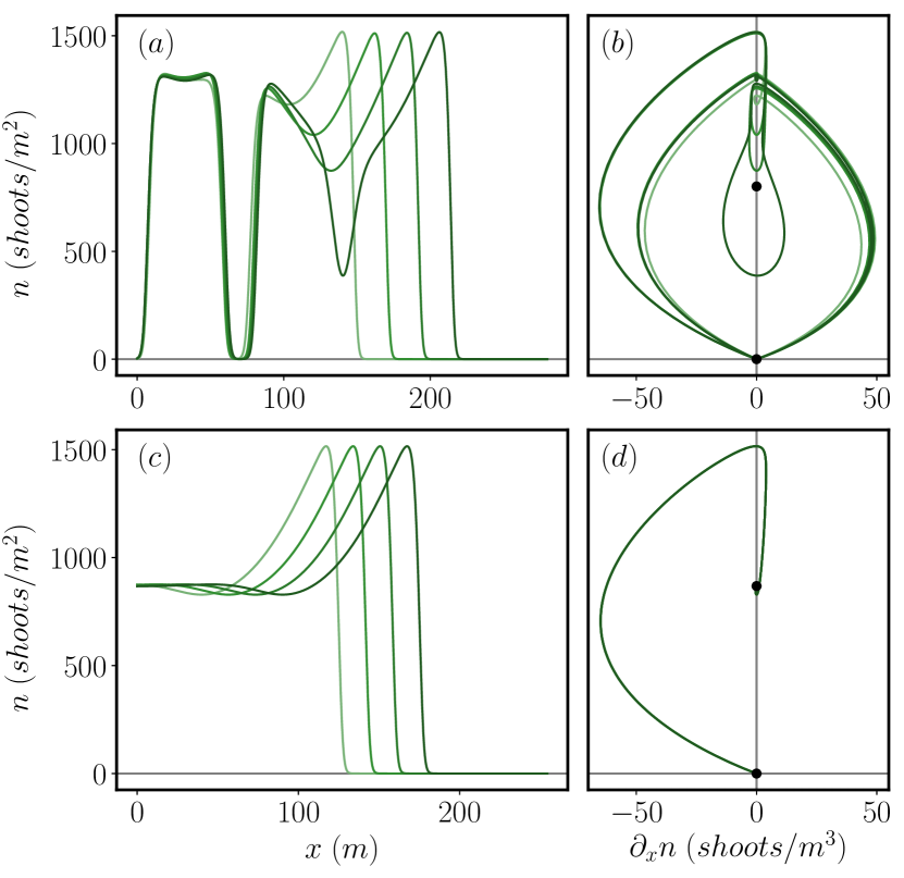
Figure 10: Spatial profiles of S-U and P-U fronts at equispaced times. Panel (a) shows the spatial profile of the density $n(x)$ across an S-U front and (b) its appearance in a $(\partial_{x}n,n)$ plot, both for $\omega_{d0}=0.0837$ $year^{-1}$ ($\omega_{d0}/\omega_{b}=1.395$). The black dots in panels (b) indicate the bare soil state U and the homogeneous populated state P. Panels (c) and (d) show the corresponding quantities for a P-U front at $\omega_{d0}=0.0758$ $year^{-1}$ ($\omega_{d0}/\omega_{b}=1.263$). The remaining parameters are as in Fig. 3.

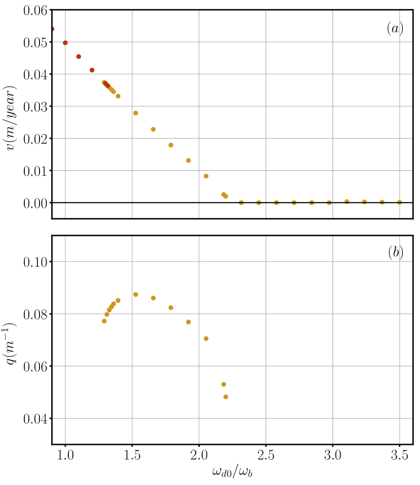
Figure 11: Speed $v$ and wavenumber $q$ of the S-U (yellow dots) front and speed $v$ of the P-U (red dots) front as a function of $\omega_{d0}/\omega_{b}$ in version I of the model. In panel (a) the speeds of the two fronts fall on the same curve, although hysteresis is present in the interval $1.277\pm 0.014\lesssim\omega_{d0}/\omega_{b}\lesssim 1.325\pm 0.008$. In panel (b) a nonzero wavenumber is selected in the interval $1.291\lesssim\omega_{d0}/\omega_{b}\lesssim 2.207$, i.e., in the interval within which the S-U front travels and is stable. Parameters as in Fig. 3.

The last front we consider is an S-P front between the stripe pattern S and the populated state P. The stability of the P state changes at the MI instability (occurring at mortality $\omega_{d0,c}$, with $\omega_{d0,c}/\omega_{b}=1.345$), whereas S is always stable in the region of coexistence with P. For $\omega_{d0}<\omega_{d0,c}$) the only possible front is pushed since both S and P are stable. As $\omega_{d0,c}/\omega_{b}$ decreases from 1.345 the speed of the pushed front also decreases and falls to zero at the right boundary of a pinning region which extends from $\omega_{d0}/\omega_{b}=1.294$ to the saddle-node bifurcation at which the S state selected by the front is created (see Fig. 3). For mortalities above MI ($\omega_{d0}/\omega_{b}>1.345$) the pushed front continues to be selected over the pulled front that now exists, until the speed of the latter exceeds that of the pushed front; thereafter the pulled front prevails (Fig. 13(a)). An example of this pulled front advancing into the P state is shown in Fig. 12. The transition from pushed to pulled takes place around $\omega_{d0,c}/\omega_{b}\approx 1.375$ where an abrupt change in the dependence of the front speed on the mortality is clearly visible. This change in the behavior of the front speed is associated with a similar change in the wavenumber of the S state deposited behind the front and the wavenumber measured at the leading edge (Fig. 13(b)). The pulled S-P front that prevails at sufficiently high mortalities remains stable until the saddle-node bifurcation $SN$ of the P state; its speed is well predicted by the linear marginal stability calculation throughout this range as is the wavenumber measured at the leading edge. Similar results have been found in other systems Hari and Nepomnyashchy (2000); Archer et al. (2014).

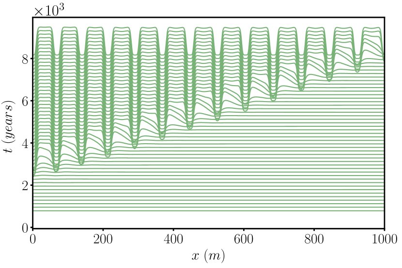
Figure 12: Space-time representation of a pulled S-P front in version I of the model. Here stable stripes S invade an unstable homogeneous state P with speed $v\approx 0.169$ $m/year$, which is well reproduced by the marginal stability calculation corresponding to a pulled front. The transient responsible for the initial thinner stripes decays rapidly leaving a well-defined stripe wavelength. Here $\omega_{d0}=0.0846$ $year^{-1}$ ($\omega_{d0}/\omega_{b}=1.41$) and the remaining parameters are as in Fig. 3.

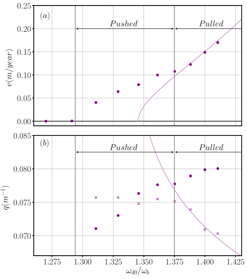
Figure 13: Speed $v$ and wavenumber $q$ of an S-P front in version I of the model as a function of $\omega_{d0}/\omega_{b}$. Dots and crosses correspond to numerical simulations while the solid line represents the linear marginal stability prediction for a pulled front. In panel (b), dots correspond to the wavenumber of the S state deposited behind the front while crosses correspond to the wavenumber measured at the leading edge. The prominent change in slope, identified by a vertical line, is associated with the transition from a pushed front to a pulled front. Parameters are as in Fig. 3.

IV.2 Fronts in version II of the model

In this section we study briefly the same fronts as in Section IV.1 but for version II of the model. The simulations are again done with a pseudospectral method, employing $\Delta t=0.167$ $years$, $\Delta x=0.025$ $m$, $N=1024$ and periodic boundary conditions. Initial fronts are formed by connecting smoothly the two desired spatially extended states. The following figures summarize the results. As before, we take $\omega_{d0}$ as the control parameter, with the other parameters as in Fig. 6.

Figure 14 shows an example of a P-U front at $\omega_{d0}/\omega_{b}=1.15$, i.e., a pushed front connecting the two homogeneous states P and U, which are both stable at this mortality value. The figure shows that P invades U. For the parameter values used the front has a constant but nonmonotonic profile and travels at constant speed $v\approx 1.091\cdot 10^{-3}$ $m/year$.

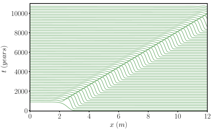
Figure 14: Space-time representation of a pushed P-U front in version II of the model, in which a stable P state invades a stable U state with speed $v\approx$ $1.091\cdot 10^{-3}$ $m/year$. Here $\omega_{d0}=0.069$ $year^{-1}$ ($\omega_{d0}/\omega_{b}=1.15$) and the remaining parameters are as in Fig. 6.

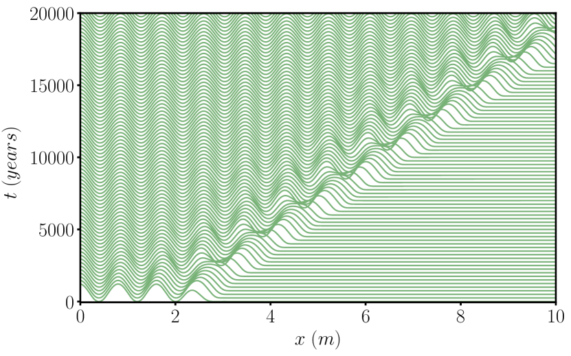
Figure 15: Space-time representation of an S-U front in version II of the model. The front travels with speed $v\approx$ $4.330\cdot 10^{-4}$ $m/year$ in the direction of S invading U. Here $\omega_{d0}=0.075$ $year^{-1}$ ($\omega_{d0}/\omega_{b}=1.25$) and the remaining parameters are as in Fig. 6.

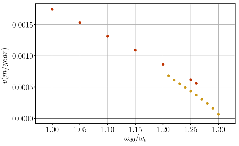
Figure 16: Speed $v$ of P-U (red symbols) and S-U (yellow symbols) fronts in version II of the model as functions of $\omega_{d0}/\omega_{b}$. Parameters are as in Fig. 6.

Figure 15 shows a space-time representation of a S-U front at $\omega_{d0}/\omega_{b}=1.25$, i.e., a front connecting the stable stripe state S to the stable bare ground state U. This is a pushed front whereby the stripe state colonizes bare ground via a time-dependent precursor that evolves into a stationary stripe pattern. For our parameter values the invasion speed $v\approx 4.330\cdot 10^{-4}$ $m/year$.

Figure 16 shows the speed of S-U fronts as a function of $\omega_{d0}/\omega_{b}$ and compares it with the speed of P-U fronts. We see that for fixed parameter values the latter travel faster, an effect we attribute to the absence of pinning.

Figure 17 shows a space-time representation of the third type of front, an S-P front connecting the stripe state S to the homogeneous populated state P at $\omega_{d0}/\omega_{b}=1.3$. Both states are stable so this is a pushed front. In contrast to version I of the model here the front invasion does not proceed with a clearly defined temporal period between successive nucleations of new stripes, which leads to a non-constant velocity. We are unsure of the reason for this. Nevertheless a mean invasion speed can be estimated and we find that $v\approx 4.419\cdot 10^{-3}$ $m/year$.

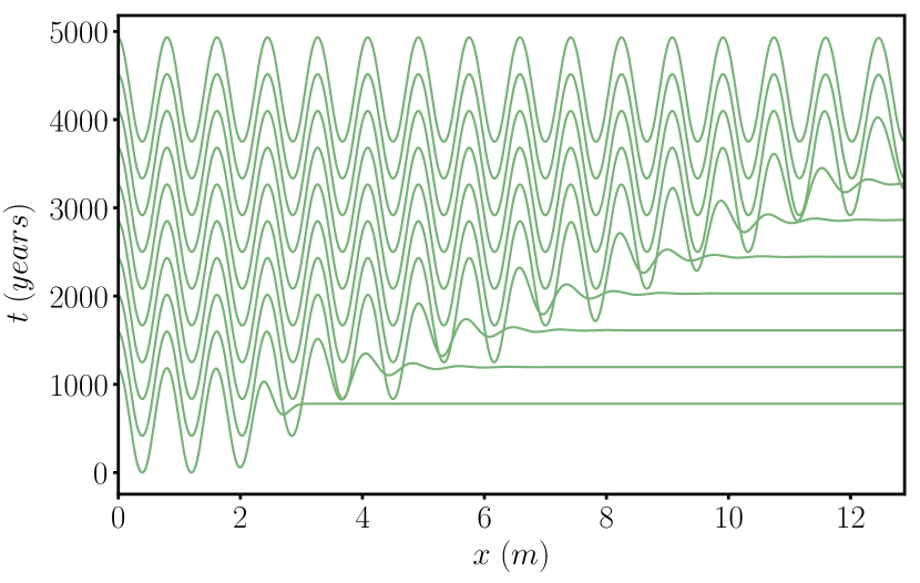
Figure 17: Space-time representation of an S-P front in version II of the model. The front travels with speed $v\approx$ $4.419\cdot 10^{-3}$ $m/year$. Here $\omega_{d0}=0.078$ $year^{-1}$ ($\omega_{d0}/\omega_{b}=1.3$) and the remaining parameters are as in Fig. 6.

Finally, Fig. 18 shows a classic example of a pinning-depinning transition associated with S-P fronts Burke and Knobloch (2006). The speed $v$ of the front decreases as one approaches the edge of the pinning region containing stationary spatially localized structures; sufficiently close to the edge the speed is expected to vary as the square root of the distance from the edge. Within the pinning region the front is self-pinned, i.e., it is pinned to the pattern state behind it, and in the depinned regime ($|v|>0$) the front is pushed until it is superseded at $\omega_{d0}/\omega_{b}\approx 1.355$ by the pulled front created in the MI.

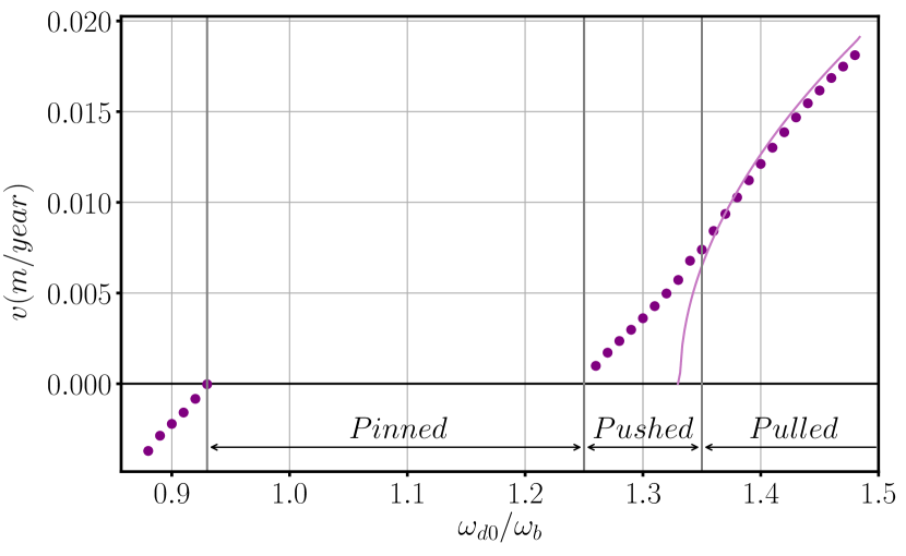
Figure 18: Speed $v$ of an S-P front in version II of the model as a function of $\omega_{d0}/\omega_{b}$, showing the pinning region in which the front is stationary. The dots correspond to numerical simulations while the solid line represents the linear marginal stability prediction for a pulled front. Parameters are as in Fig. 6.

Conclusions

We have explored two versions of a simplified model for clonal plant growth Ruiz-Reynés et al. (2020), motivated by undersea patterns observed in Posidonia oceanica meadows Ruiz-Reynés et al. (2017). The first version takes into account nonlocal competition and facilitation through appropriately formulated, albeit phenomenological kernels. The second simplifies these kernels via a gradient expansion and, after truncation, leads to a nonlinear but local evolution equation. In both cases we have taken the mortality parameter $\omega_{d0}$ as the bifurcation parameter and explored the behavior of each version as the mortality varies. In both cases we have made every effort to employ realistic values of the remaining parameters.

The key findings of our work are:

(i) There is a qualitative agreement between the nonlocal and local models in that both exhibit the same sequence of transitions between the three spatially extended states, the populated state P, the unpopulated state U and the pattern state S, as $\omega_{d0}$ varies. Nevertheless, substantial quantitative differences are seen. The nonlocal version is believed to provide more accurate predictions for the real vegetation dynamics, whereas the local approximation, because of its simpler structure, can be used as a qualitative tool to understand the transitions between different regimes.

(ii) In addition to spatially extended states both systems also exhibit two types of spatially localized structures, one resembling holes in the homogeneously populated state and the other resembling vegetation patches on bare ground, i.e., embedded in the U state. These states are organized within distinct bifurcation structures of snaking type, qualitatively similar to those arising in related local Parra-Rivas and Fernandez-Oto (2020) and nonlocal Cisternas et al. (2020) vegetation models.

(iii) Both systems exhibit a variety of fronts connecting extended states, and these may be either pushed or pulled. In the former case the speed of the front is determined by nonlinear processes while in the latter the front speed can be computed from a marginal stability criterion as described in van Saarloos (2003). In many systems, pulled fronts with marginal stability velocities are good descriptions of fronts describing stable states invading unstable states. Here we have found situations in which this is the case, but also cases in which pushed fronts prevail. The characteristic front speeds are in all cases very slow, of the order of centimeters per year, a result that is consistent with the observed slow evolution of Posidonia oceanica meadows, the case to which model parameters were fitted.

We emphasize that the results obtained here for the one-dimensional case are also relevant to the spreading of vegetation in two dimensions, since stable localized structures in one dimension block front propagation in two dimensions. However, our understanding of the dynamics of vegetation fronts based on the results of a one-dimensional analysis is necessarily limited since transverse instabilities, if present, may change both the front profile and its speed. Moreover, the presence of multiple patterns, their different orientations with respect to the front, and their different stability ranges make the analysis of fronts between patterned states in two dimensions much more challenging.

The spatial period-doubling we observe at small amplitude near the transcritical bifurcation of the U state appears to be characteristic of many vegetation models. In the present case it takes place via peak-splitting as the mortality parameter $\omega_{d0}$ increases, a process that occurs in related systems as well Yochelis et al. (2008); Zelnik et al. (2018). This process requires that near their termination the peaks that result adjust their mutual position to generate a periodic state, since only periodic states can terminate in a Turing bifurcation. Other systems exhibit spatial period division organized within a foliated snaking structure which does not require the localized structures to adjust their location Lloyd and O’Farrell (2013); Verschueren and Champneys (2017); Zelnik et al. (2017); Parra-Rivas et al. (2018b); Verschueren and Champneys (2019). Related wavelength division is found in other systems Parra-Rivas et al. (2018a). The fact that the region of stability of periodically spaced vegetation patches appears to extend all the way down to zero wavenumber (in an infinite domain) allows sensitive wavelength adaptation when parameters are varied Siteur et al. (2014).

Appendix A Marginal stability predictions for pulled P-U and S-P fronts

In this Appendix we give details of the marginal stability predictions for the velocity, and real and imaginary parts of the wavenumber of pulled P-U and S-P fronts in the two versions of the model.

A.1 Version I

We use the notation $A^{*}\equiv an^{*}e^{-an^{*}}$, $e_{\kappa}\equiv e^{-(k_{r}^{2}-k_{i}^{2})\sigma_{\kappa}^{2}/2}$ and $e_{0}\equiv e^{-(k_{r}^{2}-k_{i}^{2})\sigma_{0}^{2}/2}$, where $n^{*}$ is the constant density of a populated state P given by the solution of the equation $\omega_{b}-\omega_{d}(n^{*})=0$. The dispersion relation obtained from the linearization of version I of the model around the state $n=n^{*}$ can be used to write the condition $vk_{i}=Re[\lambda(k)]$ in the form

$$vk_{i} = -2bn^{*2}-(d_{0}+d_{1}n^{*})(k_{r}^{2}-k_{i}^{2})$$

$$-A^{*}\bigg{(}\kappa e_{\kappa}\cos(k_{r}k_{i}\sigma_{\kappa}^{2})-\omega_{d0}e_{0}\cos(k_{r}k_{i}\sigma_{0}^{2})\bigg{)}.$$

Similarly the condition $Re\left[\frac{d\lambda(k)}{dk}\right]=0$ becomes

$$0 = \bigg{(}-(d_{0}+d_{1}n^{*})$$

$$+ A^{*}\bigg{(}\kappa e_{\kappa}\cos(k_{r}k_{i}\sigma_{\kappa}^{2})\frac{\sigma_{\kappa}^{2}}{2}-\omega_{d0}e_{0}\cos(k_{r}k_{i}\sigma_{0}^{2})\frac{\sigma_{0}^{2}}{2}\bigg{)}\bigg{)}2k_{r}$$

$$+ A^{*}\bigg{(}\kappa e_{\kappa}\sin(k_{r}k_{i}\sigma_{\kappa}^{2})\frac{\sigma_{\kappa}^{2}}{2}-\omega_{d0}e_{0}\sin(k_{r}k_{i}\sigma_{0}^{2})\frac{\sigma_{0}^{2}}{2}\bigg{)}2k_{i},$$

while condition $v=-Im\left[\frac{d\lambda(k)}{dk}\right]$ takes the form

$$v = \bigg{(}+(d_{0}+d_{1}n^{*})$$

$$- A^{*}\bigg{(}\kappa e_{\kappa}\cos(k_{r}k_{i}\sigma_{\kappa}^{2})\frac{\sigma_{\kappa}^{2}}{2}-\omega_{d0}e_{0}\cos(k_{r}k_{i}\sigma_{0}^{2})\frac{\sigma_{0}^{2}}{2}\bigg{)}\bigg{)}2k_{i}$$

$$+ A^{*}\bigg{(}\kappa e_{\kappa}\sin(k_{r}k_{i}\sigma_{\kappa}^{2})\frac{\sigma_{\kappa}^{2}}{2}-\omega_{d0}e_{0}\sin(k_{r}k_{i}\sigma_{0}^{2})\frac{\sigma_{0}^{2}}{2}\bigg{)}2k_{r}.$$

These three equations are solved numerically for the unknowns $v$, $k_{r}$ and $k_{i}$ characterizing the speed and leading edge profile of a pulled front, specifically a pulled S-P front as illustrated in Fig. 13 (solid line). The same procedure around $n^{*}=0$ leads to the analytical solution $v=2\sqrt{d_{0}(\omega_{b}-\omega_{d0})}$, $k_{r}=0$ and $k_{i}=\sqrt{(\omega_{b}-\omega_{d0})/d_{0}}$ for a pulled P-U front, as illustrated in Fig. 8 (solid line).

A.2 Version II

Following the same procedure for version II the dispersion relation obtained from the linearization around $n=n^{*}$ can be written as

$$\lambda=p_{1}+p_{2}k^{2}+p_{3}k^{4},$$ (8)

where $p_{1}=\omega_{b}-\omega_{d0}-2a^{\prime}(\kappa-\omega_{b})n^{*}-3bn^{*2}$, $p_{2}=-((\alpha+d_{1})n^{*}+d_{0})$, and $p_{3}=\beta n^{*}$. Thus, the condition $vk_{i}=Re[\lambda(k)]$ can be written in the form

$$vk_{i}=p_{1}+p_{2}(k_{r}^{2}-k_{i}^{2})+p_{3}(k_{r}^{4}+k_{i}^{4}-6k_{r}^{2}k_{i}^{2}).$$ (9)

The second condition $Re\left[\frac{d\lambda(k)}{dk}\right]=0$ becomes

$$0=2k_{r}(p_{2}+2p_{3}(k_{r}^{2}-k_{i}^{2})-4p_{3}k_{i}^{2}),$$ (10)

and the last condition $v=-Im\left[\frac{d\lambda(k)}{dk}\right]$ takes the form

$$v=-2k_{i}(p_{2}+2p_{3}(k_{r}^{2}-k_{i}^{2})+4p_{3}k_{i}^{2}).$$ (11)

The velocity of a front between stripes and the homogeneous solution can be computed in the case where $k_{r}\neq 0$, where

$$k_{r}=\pm\sqrt{\frac{-3p_{2}\pm\sqrt{7p_{2}^{2}-24p_{1}p_{3}}}{8p_{3}}}.$$ (12)

The imaginary part $k_{i}$ can be computed using the expression

$$k_{i}=\pm\sqrt{\frac{p_{2}+2p_{3}k_{r}^{2}}{6p_{3}}}.$$ (13)

In terms of these quantities the speed $v$ is given by

$$v=-8k_{i}p_{3}(k_{r}^{2}+k_{i}^{2}).$$ (14)

The last expression is used to compute the velocity of a pulled S-P front, which is represented in Fig. 18. The velocity of a P-U front can be obtained from a linearization around $n^{*}=0$, which leads to the same expressions as in version I of the model.

References

- Meron (2015) E. Meron, Nonlinear Physics of Ecosystems (CRC Press, Boca Raton, 2015).
- Rietkerk et al. (2004) M. Rietkerk, S. C. Dekker, P. C. de Ruiter, and J. van de Koppel, Science 305, 1926 (2004).
- Barbier et al. (2006) N. Barbier, P. Couteron, J. Lejoly, V. Deblauwe, and O. Lejeune, Journal of Ecology 94, 537 (2006).
- Watt (1947) A. S. Watt, Journal of Ecology 35, 1 (1947).
- Rietkerk and van de Koppel (2008) M. Rietkerk and J. van de Koppel, Trends in Ecology & Evolution 23, 169 (2008).
- Meron (2012) E. Meron, Ecological Modelling 234, 70 (2012).
- Ruiz-Reynés et al. (2017) D. Ruiz-Reynés, D. Gomila, T. Sintes, E. Hernández-García, N. Marbà, and C. M. Duarte, Science Advances 3, e1603262 (2017), arXiv:1709.01072 .
- von Hardenberg et al. (2001) J. von Hardenberg, E. Meron, M. Shachak, and Y. Zarmi, Phys. Rev. Lett. 87, 198101 (2001).
- Gilad et al. (2007a) E. Gilad, J. von Hardenberg, A. Provenzale, M. Shachak, and E. Meron, Journal of Theoretical Biology 244, 680 (2007a).
- Gilad et al. (2007b) E. Gilad, M. Shachak, and E. Meron, Theoretical Population Biology 72, 214 (2007b).
- Gandhi et al. (2018) P. Gandhi, L. Werner, S. Iams, K. Gowda, and M. Silber, Journal of the Royal Society, Interface 15, 20180508 (2018).
- Lefever and Lejeune (1997) R. Lefever and O. Lejeune, Bulletin of Mathematical Biology 59, 263 (1997).
- Martínez-García et al. (2013) R. Martínez-García, J. M. Calabrese, E. Hernández-García, and C. López, Geophysical Research Letters 40, 6143 (2013), arXiv:1308.1810 .
- Martínez-García et al. (2014) R. Martínez-García, J. M. Calabrese, E. Hernández-García, and C. López, Philosophical Transactions of the Royal Society A: Mathematical, Physical and Engineering Sciences 372, 20140068 (2014).
- Fernandez-Oto et al. (2014) C. Fernandez-Oto, M. Tlidi, D. Escaff, and M. G. Clerc, Philosophical Transactions of the Royal Society A: Mathematical, Physical and Engineering Sciences 372, 20140009 (2014), arXiv:1306.4848 .
- Cisternas et al. (2020) J. Cisternas, D. Escaff, M. G. Clerc, R. Lefever, and M. Tlidi, Chaos, Solitons & Fractals 133, 109617 (2020).
- Ruiz-Reynés and Gomila (2019) D. Ruiz-Reynés and D. Gomila, Phys. Rev. E 100, 1 (2019).
- Ruiz-Reynés et al. (2020) D. Ruiz-Reynés, F. Schönsberg, E. Hernández-García, and D. Gomila, Physical Review Research 2, 023402 (2020).
- Alvarez-Socorro et al. (2017) A. J. Alvarez-Socorro, M. G. Clerc, G. González-Cortés, and M. Wilson, Phys. Rev. E 95, 010202 (2017).
- Fernandez-Oto et al. (2019) C. Fernandez-Oto, O. Tzuk, and E. Meron, Phys. Rev. Lett. 122, 048101 (2019).
- Parra-Rivas and Fernandez-Oto (2020) P. Parra-Rivas and C. Fernandez-Oto, Phys. Rev. E 101, 052214 (2020).
- Keller (1986) H. B. Keller, SIAM Review (Springer-Verlag, 1986).
- Mittelmann (1986) H. D. Mittelmann, SIAM Journal on Numerical Analysis 23, 1007 (1986).
- Woods and Champneys (1999) P. D. Woods and A. R. Champneys, Physica D 129, 147 (1999).
- Coullet et al. (2000) P. Coullet, C. Riera, and C. Tresser, Phys. Rev. Lett. 84, 3069 (2000).
- Burke and Knobloch (2006) J. Burke and E. Knobloch, Phys. Rev. E 73, 56211 (2006).
- Mercader et al. (2013) I. Mercader, O. Batiste, A. Alonso, and E. Knobloch, Journal of Fluid Mechanics 722, 240 (2013).
- Champneys et al. (2012) A. R. Champneys, E. Knobloch, Y.-P. Ma, and T. Wagenknecht, SIAM Journal on Applied Dynamical Systems 11, 1583 (2012).
- Yochelis et al. (2008) A. Yochelis, Y. Tintut, L. L. Demer, and A. Garfinkel, New Journal of Physics 10, 055002 (2008).
- Parra-Rivas et al. (2018a) P. Parra-Rivas, D. Gomila, L. Gelens, and E. Knobloch, Phys. Rev. E 98, 042212 (2018a), arXiv:1805.02555 .
- Doelman et al. (1998) A. Doelman, R. A. Gardner, and T. J. Kaper, Physica D 122, 1 (1998).
- Doelman et al. (2012) A. Doelman, J. D. M. Rademacher, and S. Van Der Stelt, Discrete and Continuous Dynamical Systems - Series S 5, 61 (2012).
- Zelnik et al. (2018) Y. R. Zelnik, P. Gandhi, E. Knobloch, and E. Meron, Chaos: An Interdisciplinary Journal of Nonlinear Science 28, 033609 (2018).
- van Saarloos (2003) W. van Saarloos, Physics Reports 386, 29 (2003), arXiv:0308540 [cond-mat] .
- Hari and Nepomnyashchy (2000) A. Hari and A. A. Nepomnyashchy, Phys. Rev. E 61, 4835 (2000).
- Archer et al. (2014) A. J. Archer, M. C. Walters, U. Thiele, and E. Knobloch, Phys. Rev. E 90, 042404 (2014).
- van Saarloos and Hohenberg (1992) W. van Saarloos and P. C. Hohenberg, Physica D 56, 303 (1992).
- Holzer and Scheel (2014) M. Holzer and A. Scheel, SIAM Journal on Mathematical Analysis 46, 397 (2014).
- Gelens et al. (2010) L. Gelens, D. Gomila, G. Van Der Sande, M. A. Matías, and P. Colet, Phys. Rev. Lett. 104, 1 (2010).
- Fernandez-Oto et al. (2013) C. Fernandez-Oto, M. G. Clerc, D. Escaff, and M. Tlidi, Phys. Rev. Lett. 110, 174101 (2013).
- Lloyd and O’Farrell (2013) D. J. Lloyd and H. O’Farrell, Physica D 253, 23 (2013).
- Verschueren and Champneys (2017) N. Verschueren and A. Champneys, SIAM Journal on Applied Dynamical Systems 16, 1797 (2017).
- Zelnik et al. (2017) Y. R. Zelnik, H. Uecker, U. Feudel, and E. Meron, Journal of Theoretical Biology 418, 27 (2017).
- Parra-Rivas et al. (2018b) P. Parra-Rivas, D. Gomila, L. Gelens, and E. Knobloch, Phys. Rev. E 97, 042204 (2018b), arXiv:1801.04796 .
- Verschueren and Champneys (2019) N. Verschueren and A. Champneys, preprint arXiv:1809.07847 (2019).
- Siteur et al. (2014) K. Siteur, E. Siero, M. B. Eppinga, J. D. M. Rademacher, A. Doelman, and M. Rietkerk, Ecological Complexity 20, 81 (2014).