Ernest Henley and the shape of baryons

Abstract

Calculations of pion-baryon couplings, baryon quadrupole and octupole moments, baryon spin and orbital angular momentum done in collaboration with Ernest Henley are reviewed. A common theme of this work is the shape of baryons. Also, a personal account of my work with Ernest Henley during the period 1999-2013 is given.

I Introduction

Before reviewing the work I did with Ernest Henley, I would like to recount some personal memories of how I came to know him and how it came about that we worked together on baryon properties for over a decade.

During the academic year 1980/1981, I and two fellow students from the University of Mainz were exchange students at the University of Washington in Seattle. One of them told me that with the credits transfered from our German home University we could get a Bachelor’s degree from the University of Washington within one year. Both of us managed to obtain the required additional credits. In August 1981 we received the desired Bachelor of Science diploma signed by the Dean of the Faculty of Arts and Sciences, Ernest Henley. At that time, he was not lecturing and I did not come to know him personally.

After returning to the University of Mainz, I took my Master’s exams, and in the following semester, started to work on my Master’s thesis on meson exchange currents with Hartmuth Arenhövel. The textbook ”Subatomic Physics” by Frauenfelder and Henley Fra74 was an invaluable guide during my thesis work and beyond and became one of my favorite textbooks.

In 1984 Prof. Henley was awarded the prestigious Humboldt prize that allowed him to travel and teach at various German universities. It so happened that in September 1984 he gave a series of lectures on electroweak interactions at the Students’ Workshop held in the small town of Bosen near Mainz. One afternoon, while walking together around the Bostal lake, I told him about my Master’s thesis on meson exchange current operators that had to be constructed so as to satisfy the continuity equation consistently with the nucleon-nucleon interaction potential Buc85 . Ernest was very encouraging and said that focusing on the continuity equation was very important to obtain reliable results.

One evening during the Bosen workshop, there was a performance of a fire artist spitting flames and juggling with fiery rings. I happened to be standing next to Ernest and made a snobbish remark saying something like ”…if he only would apply his skills to something more useful…”. Ernest looked at me and said: ”Why, he is entertaining people. That is allright.” This was only one of several occasions, where I noticed that he treated everybody with respect.

Another story characteristic of Ernest’s modesty was related to me by Lothar Tiator, who was coorganizer of the Bosen workshop. At the time Humboldt prize winners were provided with a BMW car free of charge during their stay in Germany. Ernest’s first reaction was: ”I would have prefered a bicycle”.

Figure 1: Participants of the Students’ Workshop in Bosen in 1984. The author is holding a notebook.
Courtesy of Dr. Lothar Tiator.

As a Humboldt fellow, Ernest Henley often visited the University of Tübingen during the period 1984-2000. I was working on my PhD thesis there and as a postdoc with Amand Fäßler. That is when I learned that Ernest was born in Frankfurt, close to Mainz where I was born. When he spoke German, you could hear traces of the regional accent typical for this area. During his visits in the late nineties, we had some discussions on relations between baryon charge radii and quadrupole moments that Eliecer Hernández, Amand Fäßler, and myself had obtained in a quark model including two-body exchange currents Buc97 . Early in 1999, G. Dillon and G. Morpurgo had rederived the relation between proton, neutron and $\Delta^{+}$ charge radii using a model-independent QCD parameterization technique Dil99a .

Ernest immediatedly realized the virtue of the Morpurgo method Mor89 ; Mor92 and its potential applicability to baryon quadrupole moments and other observables. So it came about that Ernest invited me to the University of Washington in the fall of 1999 for a month. There we laid the ground work for several papershen00a ; hen00b ; Hen02 ; Hen08 ; Hen11 ; Hen14 which were published between 2000 and 2014. Ernest noticed that pion-baryon couplings had not yet been calculated with this method and suggested that we do this first hen00a . During my stay, Ernest generously shared his office with me, invited me over for dinner, and on the last day he insisted that he drive me to the airport very early in the morning.

Thereafter we continued our collaboration by email and by visiting each other either in Seattle or Tübingen. During my visit to Seattle in 2005, we started our work on baryon magnetic octupole moments Hen08 , a topic which Ernest was particularly fond of.

In the spring of 2010, while staying in Munich he called me, and we managed to meet and discuss physics for several hours in the DB lounge at the Munich Central train station. That is when we started our last collaboration on the proton spin problem Hen11 ; Hen14 at his suggestion. Back in 1999, when we first began working together, he had already mentioned that the nucleon shape issue was closely related with the proton spin problem. During the meeting in Munich, we realized how to apply Morpurgo’s method to calculate quark spin and quark orbital angular momentum.

Without Ernest’s profound knowledge, creativity, and persistence, the following results would not have been possible.

II Morpurgo’s general parameterization method

In 1989 Morpurgo Mor89 ; Mor92 introduced a general parameterization (GP) method for the properties of baryons, which expresses masses, magnetic moments, transition amplitudes, and other properties of the baryon octet and decuplet in terms of a few parameters. The method uses only general features of QCD and baryon descriptions in terms of quarks. Later, Dillon and Morpurgo showed that the method is independent of the choice of the quark mass renormalization point in the QCD Lagrangian Dil96 . Dillon and Morpurgo also extended the method to nucleon charge radii Dil99a and electromagnetic form factors Dil99b .

The Morpurgo method is based on the following considerations. For the observable at hand one formally writes a QCD operator $\Omega$ and QCD eigenstates expressed explicitly in terms of quarks and gluons. This matrix element can, with the help of the unitary operator $V$, be expressed in the basis of auxiliary (model) three-quark states $\Phi_{B}$

$$\left\langle B|\Omega|B\right\rangle=\left\langle\Phi_{B}|V^{\dagger}\Omega V|\Phi_{B}\right\rangle=\left\langle W_{B}|{\cal O}|W_{B}\right\rangle\,.$$ (1)

Both the unitary operator $V$ and the model states $\Phi_{B}$ are defined in Ref.Mor89 . The $\Phi_{B}$ are pure $L=0$ three-quark states excluding any quark-antiquark or gluon components. $W_{B}$ stands for the standard three-quark $SU(6)$ spin-flavor wave functions Clo . The operator $V$ dresses the auxiliary states $\Phi_{B}$ with $q\bar{q}$ components and gluons and thereby generates the exact QCD eigenstate $|B\rangle$ as in

$$|B\rangle = \alpha|qqq\rangle+\beta_{1}|qqq\,(q\overline{q})\rangle+\beta_{2}|qqq\,(q\overline{q})^{2}\rangle+$$ (2)

$$\ldots+\gamma_{1}|qqq\,g\rangle+\gamma_{2}|qqq\,gg\rangle+\ldots$$

On the right hand side of the last equality in Eq.(1) the integration over spatial and color degrees of freedom has been performed. As a result only a matrix element of a spin-flavor operator $\mathcal{O}$ between spin-flavor states $|W_{B}\rangle$ remains. The $q{\bar{q}}$ and gluon degrees of freedom of the exact QCD eigenstates now appear as many-quark operators, constrained by Lorentz and inner QCD symmetries. Although non-covariant in appearance, the operator basis of this method involves a complete set of spin-flavor invariants that are allowed by Lorentz invariance and flavor symmetry.

One then writes the most general expression for ${\cal O}$ compatible with the space-time and inner QCD symmetries. Generally, this is a sum of one-, two-, and three-quark operators in spin-flavor space multiplied by a priori unknown constants $A_{1}$, $A_{2}$, and $A_{3}$ which parametrize the orbital and color space matrix elements. Empirically, a hierarchy in the importance of one-, two-, and three-quark operators is found. This fact can be understood in the $1/N_{c}$ expansion Das94 where two- and three-quark operators describing second and third order SU(6) symmetry breaking are usually suppressed by powers of $1/N_{c}$ and $1/N_{c}^{2}$ respectively, compared to one-quark operators associated with first order symmetry breaking Leb00 ; Leb02 .

III Pion-baryon couplings

For the strong pion-baryon couplings one-, two-, and three-quark axial vector operators are defined as hen00a ; mos13

$${\mathcal{O}}_{1} = A_{1}\,\sum_{i=1}^{3}\tau_{3}^{i}\sigma_{z}^{i},$$

$${\mathcal{O}}_{2} = A_{2}\,\sum_{i\neq j=1}^{3}\tau_{3}^{i}\sigma_{z}^{j}$$

$${\mathcal{O}_{3}} = A_{3}\,\sum_{i\neq j\neq k=1}^{3}\,\tau_{3}^{i}\,\sigma_{z}^{i}\,{\mbox{\boldmath$\sigma$}}^{j}\cdot{\mbox{\boldmath$\sigma$}}^{k},$$ (3)

and the total operator reads

$${\mathcal{O}}={\mathcal{O}}_{1}+{\mathcal{O}}_{2}+{\mathcal{O}}_{3}.$$ (4)

Here, ${\mbox{\boldmath$\sigma$}}^{i}$ and ${\mbox{\boldmath$\tau$}}^{i}$ are the spin and isospin operators of quark $i$.

These operators are evaluated using completely symmetric symmetric spin-isospin states $|W_{B}\rangle$ Clo . We obtained the quark model matrix elements up to second order corrections (two-body terms) listed in Table 1, where $r=\frac{m_{u}}{m_{s}}$, is a flavor symmetry breaking parameter included in the two-body term, with $m_{u}=m_{d}$ and $m_{s}$ being the masses of non-strange and strange quarks.

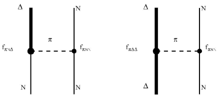
Figure 2: Strong coupling of the pion to the nucleon ($N$) and $\Delta$-isobar ($\Delta$). The $\pi NN$, $\pi N\Delta$, and $\pi\Delta\Delta$ coupling constants are denoted as $f_{\pi NN}$, $f_{\pi N\Delta}$, and $f_{\pi\Delta\Delta}$. The corresponding interaction vertices are represented as black dots.

Table 1: Quark model matrix elements of the operator in Eq.(4) to first order (${\mathcal{O}}_{1}$) and second order corrections (${\mathcal{O}}_{2}$).

Baryon	First order	Second order
p	$\frac{5}{3}A_{1}$	-$\frac{2}{3}A_{2}$
$\Sigma^{+}$	$\frac{4}{3}A_{1}$	$\frac{2(2-r)}{3}A_{2}$
$\Sigma^{0}\rightarrow\Lambda^{0}$	$-\frac{2\sqrt{3}}{3}A_{1}$	$\frac{2\sqrt{3}}{3}A_{2}$
$\Xi^{0}$	$-\frac{1}{3}A_{1}$	$\frac{4\,r}{3}A_{2}$
$\Delta^{+}\rightarrow p$	$\frac{4\sqrt{2}}{3}A_{1}$	- $\frac{4\sqrt{2}}{3}A_{2}$
$\Sigma^{*+}\rightarrow\Sigma^{+}$	$\frac{2\sqrt{2}}{3}A_{1}$	$\frac{2\sqrt{2}(1-2r)}{3}A_{2}$
$\Sigma^{*0}\rightarrow\Lambda^{0}$	$\frac{2\sqrt{6}}{3}A_{1}$	$-\frac{2\sqrt{6}}{3}A_{2}$
$\Xi^{*0}\rightarrow\Xi^{0}$	$\frac{2\sqrt{2}}{3}A_{1}$	$-\frac{2\sqrt{2}\,r}{3}A_{2}$
$\Delta^{+}$	$A_{1}$	$2A_{2}$
$\Sigma^{*+}$	$2A_{1}$	$2(1+r)A_{2}$
$\Xi^{*0}$	$A_{1}$	$2rA_{2}$

To derive from the quark level matrix elements in Table 1 the conventional pion-baryon couplings Bro75 , as depicted in Fig. 2 for the nucleon (N) and $\Delta$ the quark level matrix elements must be divided by baryon level spin and isospin Clebsch-Gordan coefficients hen00a ; mos13 . Table 2 lists the various couplings in terms of $\,f\,$, the $\pi^{0}p$ coupling constant, to first order and to second order with and without the inclusion of the SU(3) flavor symmetry breaking parameter $r=m_{u}/m_{s}$.

Table 2: Coupling constants of the pion to various members of the baryon octet and decuplet, and the decuplet-octet transitions in terms of $f=f_{\pi^{0}pp}$. The * indicates an input. The ratio $r=m_{u}/m_{s}$ of non-strange and strange quark masses indicates the degree of flavor symmetry breaking.

Baryon	First order	Total	Total
	($A_{2}=0$)	r=1	r=0.6
p	1	1	1
$\Sigma^{+}$	0.80	0.59	0.54
$\Sigma^{0}\rightarrow\Lambda^{0}$	-0.69	-0.82	-0.82
$\Xi^{0}$	-0.20	-0.42	-0.32
$\Delta^{+}\rightarrow p$	1.70	2*	2*
$\Sigma^{*+}\rightarrow\Sigma^{+}$	0.98	1.16	0.92
$\Sigma^{*0}\rightarrow\Lambda^{0}$	-1.20	-1.42	-1.42
$\Xi^{*0}\rightarrow\Xi^{0}$	-1.20	-1.42	-1.28
$\Delta^{+}$	0.80	0.23	0.23
$\Sigma^{*+}$	0.80	0.23	0.32
$\Xi^{*0}$	0.80	0.23	0.42

Our results satisfy the following relation in the SU(3) symmetric case

$$f_{\pi^{0}pp}+f_{\pi^{0}\Xi^{0}\Xi^{0}} = f_{\pi^{0}\Sigma^{+}\Sigma^{+}}\;.$$ (5)

Furthermore, the $\pi\Sigma\Lambda$ and the $\pi\Sigma^{*}\Lambda$ couplings remain unaffected by SU(3) symmetry breaking. Irrespective of the value of $r$ the octet-decuplet transition couplings satisfy the sum rule

$$\sqrt{2}f_{\Delta^{+}p}=f_{\Xi^{*0}\Xi^{0}}+\sqrt{6}f_{\Sigma^{*+}\Sigma^{+}}-f_{\Sigma^{*0}\Lambda^{0}}.$$ (6)

This relation is not new. It has been derived before Bec64 using SU(3) symmetry and its breaking to first order.

In addition, by taking ratios of two transition couplings for $\pi^{+}$ emission we got for the case $r=1$

$$\frac{f_{{\Delta^{++}p}}}{f_{\Sigma^{*+}\Sigma^{0}}}=-\sqrt{6}\,(-3.06),\quad\frac{f_{\Sigma^{*+}\Sigma^{0}}}{f_{\Sigma^{*+}\Lambda^{0}}}=-\frac{1}{\sqrt{3}}\,(-0.46)$$ (7)

The numbers in parentheses include SU(3) symmetry breaking in the two-quark term $(r=0.6)$. These results are in agreement with those obtained in the large $N_{c}$ approach Das94 , including the next-to-leading order corrections, which is undoubtedly more than a numerical coincidence.

Finally, we found certain analytical relations between octet and decuplet baryon couplings to pions (neglecting three-quark terms)

$$f_{\pi^{0}p}-\frac{1}{4}f_{\pi^{0}\Delta^{+}\Delta^{+}} = \frac{\sqrt{2}}{3}f_{\pi^{0}p\Delta^{+}}$$

$$f_{\pi^{0}\Sigma^{+}}-\frac{1}{2}f_{\pi^{0}\Sigma^{*+}\Sigma^{*+}} = \frac{1}{\sqrt{6}}f_{\pi^{0}\Sigma^{*+}\Sigma^{+}}$$

$$f_{\pi^{0}\Xi^{0}}-\frac{1}{4}f_{\pi^{0}\Xi^{*0}\Xi^{*0}} = \frac{1}{3}f_{\pi^{0}\Xi^{*0}\Xi^{0}}.$$ (8)

They are a consequence of the underlying unitary symmetry, and are valid for all values of the strange quark mass. Eq.(III) can be used to predict the elusive decuplet couplings from the experimentally better known octet and decuplet-octet transition couplings. As far as we know, these relations are new.

Including the three-body term for the nucleon and $\Delta$, Steve Moszkowski and myself later found that the first relation in Eq.(III) is modified. It turned out that three-quark terms have a major effect on the $\pi\Delta\Delta$ coupling and the reduction of the $\pi\Delta\Delta$ coupling obtained in second order is more than compensated by the inclusion of third order symmetry breaking term mos13 . We also found an interesting connection between the $\pi NN$, $\pi N\Delta$ and $\pi\Delta\Delta$ couplings and the shape of the $N$ and $\Delta$.

IV Intrinsic quadrupole moment of the nucleon

To learn something about the shape of a spatially extended particle one has to determine its intrinsic quadrupole moment Boh75

$$Q_{0}=\int d^{3}r\rho({\bf r})(3z^{2}-r^{2}),$$ (9)

which is defined with respect to the body-fixed frame and thus defines the shape of the particle. If $Q_{0}>0$ the particle is prolate (cigar-shaped), if $Q_{0}<0$ the particle is oblate (pancake-shaped).

The intrinsic quadrupole moment $Q_{0}$ must be distinguished from the spectroscopic quadrupole moment $Q$ measured in the laboratory frame. Due to angular momentum selection rules, a spin $J=1/2$ nucleus, such as the nucleon, does not have a spectroscopic quadrupole moment. This is analogous to a deformed $J=1/2$ or $J=0$ nucleus. For example, all orientations of a deformed $J=0$ nucleus are equally probable, which results in a spherical charge distribution in the ground state and a vanishing quadrupole moment $Q$ in the laboratory.

The intrinsic quadrupole moment $Q_{0}$ of a spin $J=1/2$ can then only be obtained by measuring electromagnetic quadrupole transitions between the ground and excited states, or by measuring the quadrupole moment of an excited state with $J>1/2$ of that nucleus.

During my stay in Seattle in 1999, Ernest and I discussed how to extract from the measured $N\to\Delta$ transition quadrupole moment the proton’s intrinsic quadrupole moment, which contains the relevant information on the proton shape. We had noticed that most work that addressed the issue of nucleon deformation Gia79 ; Ven81 ; Ma83 ; Cle84 ; Mig87 did not clearly distinguish between intrinsic (body-fixed frame) and the measured spectroscopic (laboratory) quadrupole moment as qualitatively shown in Fig. 3.

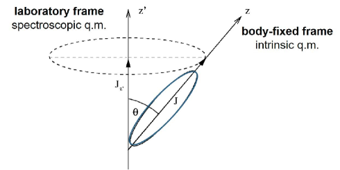
Figure 3: Precession of a semiclassical deformed charge distribution with intrinsic symmetry axis $z$ and spin $J$ around the laboratory frame $z^{\prime}$ axis. The transformation from the body-fixed to the laboratory frame gives rise to a projection factor $P_{2}(\cos(\Theta))=(3\,\cos^{2}(\Theta)-1)/2$ relating the spectroscopic quadrupole moment $Q$ (laboratory frame) and the intrinsic quadrupole moment $Q_{0}$ (body-fixed frame) as $Q=[(3J_{z}^{\prime 2}-J(J+1))/(2J(J+1))]Q_{0}$, where $J$ is the total angular momentum, and $J_{z}^{\prime}$ its projection on the $z^{\prime}$ axis. For $J=0$ and $J=1/2$ systems, $Q=0$ even if $Q_{0}\neq 0$. It is $Q_{0}$ and not $Q$ that pertains to the shape of the system.

IV.1 Quark model

In standard notation the $SU(6)$ spin-flavor wave function of the proton is composed of a spin-singlet and a spin-triplet term for the coupling of the first two quarks

$$|p\rangle = {1\over\sqrt{2}}\biggl{\{}{1\over\sqrt{6}}|\left(2uud-udu-duu\right)\rangle$$ (10)

$$\times {1\over\sqrt{6}}\left(2\uparrow\uparrow\downarrow-\uparrow\downarrow\uparrow-\downarrow\uparrow\uparrow\right)\rangle$$

$$+{1\over\sqrt{2}}|\left(udu-duu\right)\rangle|{1\over\sqrt{2}}\left(\uparrow\downarrow\uparrow-\downarrow\uparrow\uparrow\right)\rangle\biggr{\}}.$$

The angular momentum coupling factors $2$, $-1$, $-1$ in front of the three terms in the spin triplet part express (i) the coupling of the first two quarks to an $S=1$ diquark, and (ii) the coupling of the $S=1$ diquark with the third quark to total $J=1/2$.

In leading order, the quadrupole moment is a two-quark operator in spin-flavor space

$${\hat{Q}}_{[2]}=B\sum_{i\neq j=1}^{3}e_{i}\left(3\sigma_{i\,z}\sigma_{j\,z}-{\hbox{$\sigma$}\hbox to0.0pt{\hss\hbox{$\sigma$}\hskip 0.39993pt}\hbox to0.0pt{\hss\lower 0.17218pt\hbox{\hbox{$\sigma$}\hbox to0.0pt{\hss\hbox{$\sigma$}\hskip 0.39993pt}}}}_{i}\cdot{\hbox{$\sigma$}\hbox to0.0pt{\hss\hbox{$\sigma$}\hskip 0.39993pt}\hbox to0.0pt{\hss\lower 0.17218pt\hbox{\hbox{$\sigma$}\hbox to0.0pt{\hss\hbox{$\sigma$}\hskip 0.39993pt}}}}_{j}\right),$$ (11)

where $e_{i}=(1+3\tau_{i\,z})/6$ is the charge of the i-th quark, and the $z$-component of the Pauli spin (isospin) matrix $\hbox{$\sigma$}\hbox to0.0pt{\hss\hbox{$\sigma$}\hskip 0.39993pt}\hbox to0.0pt{\hss\lower 0.17218pt\hbox{\hbox{$\sigma$}\hbox to0.0pt{\hss\hbox{$\sigma$}\hskip 0.39993pt}}}_{i}$ ($\hbox{$\tau$}\hbox to0.0pt{\hss\hbox{$\tau$}\hskip 0.39993pt}\hbox to0.0pt{\hss\lower 0.17218pt\hbox{\hbox{$\tau$}\hbox to0.0pt{\hss\hbox{$\tau$}\hskip 0.39993pt}}}_{i}$) is denoted by $\sigma_{i\,z}$ ($\tau_{i\,z}$). The constant $B$ with dimension fm² contains the orbital and color matrix elements. There is no one-quark operator, because one cannot construct a spin tensor of rank 2 from a single Pauli matrix.

Sandwiching the quadrupole operator ${\hat{Q}}_{[2]}$ between the proton’s spin-flavor wave function yields a vanishing spectroscopic quadrupole moment. The reason is clear. The spin tensor ${\hat{Q}}_{[2]}$ applied to the spin-singlet wave function gives zero, and when acting on the proton’s spin-triplet wave function it gives

$$\left(3\sigma_{1\,z}\sigma_{2\,z}-\hbox{$\sigma$}\hbox to0.0pt{\hss\hbox{$\sigma$}\hskip 0.39993pt}\hbox to0.0pt{\hss\lower 0.17218pt\hbox{\hbox{$\sigma$}\hbox to0.0pt{\hss\hbox{$\sigma$}\hskip 0.39993pt}}}_{1}\cdot\hbox{$\sigma$}\hbox to0.0pt{\hss\hbox{$\sigma$}\hskip 0.39993pt}\hbox to0.0pt{\hss\lower 0.17218pt\hbox{\hbox{$\sigma$}\hbox to0.0pt{\hss\hbox{$\sigma$}\hskip 0.39993pt}}}_{2}\right){1\over\sqrt{6}}\left|\left(2\uparrow\uparrow\downarrow-\uparrow\downarrow\uparrow-\downarrow\uparrow\uparrow\right)\right\rangle$$ (12)

$$= {4\over\sqrt{6}}|\left(\uparrow\uparrow\downarrow+\uparrow\downarrow\uparrow+\downarrow\uparrow\uparrow\right)\rangle,$$

where the right-hand side is a spin 3/2 wave function, which has zero overlap with the spin 1/2 wave function of the proton in the final state. Consequently, the spectroscopic quadrupole moment

$$Q_{p}=\langle p|\hat{Q}_{[2]}|p\rangle=B\left(2-1-1\right)=0$$ (13)

vanishes due to the spin coupling coefficients in $|p\rangle$.

Although the spin $S=1$ diquarks ($uu$ and $ud$) in the proton have nonvanishing quadrupole moments, the angular momentum coupling of the diquark spin to the spin of the third quark prevents this quadrupole moment from being observed.

Ernest came up with the idea to renormalize the Clebsch-Gordan coefficients in spin space that guarantee that the proton spectroscopic quadrupole moment is zero hen00b . Setting “by hand” all Clebsch-Gordan coefficients in the spin part of the proton wave function of Eq.(10) equal to 1, while preserving the normalization, one obtains a modified “proton” wave function $|{\tilde{p}}\rangle$

$$|{\tilde{p}}\rangle = {1\over\sqrt{2}}\biggl{\{}\biggl{[}|{1\over\sqrt{6}}\left(2uud-udu-duu\right)\rangle$$ (14)

$$+ {1\over\sqrt{2}}|\left(udu-duu\right)\rangle\biggr{]}$$

$$\times {1\over\sqrt{3}}|\left(\uparrow\uparrow\downarrow+\uparrow\downarrow\uparrow+\downarrow\uparrow\uparrow\right)\rangle\biggr{\}}.$$

The renormalization of the Clebsch-Gordan coefficients is undoing the averaging over all spin directions, which renders the intrinsic quadrupole moment unobservable. We did not modify the flavor part of the wave function in order to ensure that we deal with a proton.

We considered the expectation value of the two-body quadrupole operator ${\hat{Q}}_{[2]}$ in the state of the spin-renormalized proton wave function $|\tilde{p}\rangle$ as an estimate of the intrinsic quadrupole moment of the proton $Q_{0}^{p}$

$$Q_{0}^{p}=\langle{\tilde{p}}|Q_{[2]}|{\tilde{p}}\rangle=2B\left(\frac{2}{3}-\frac{8}{3}\right)=-4B=-r_{n}^{2}.$$ (15)

The two terms in Eq.(15) arise from the spin 1 diquark with projection $M=1$ and $M=0$. The latter dominates. The last equality came from a comparison with the quark model relation Buc97 that was rederived with fewer assumptions hen00b

$$\sqrt{2}Q_{p\to\Delta^{+}}=Q_{\Delta^{+}}=r_{n}^{2}=4B.$$ (16)

This relation is in good agreement with experimental data Bla01 ; Tia03 . Thus, we found that the intrinsic quadrupole moment of the proton, $Q_{0}^{p}$ is equal to the negative of the neutron charge radius $r_{n}^{2}$ and is therefore positive.

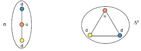
Figure 4: Left: In the neutron, both down quarks are in a spin 1 state, and are repelled more strongly than an up-down pair. This results in an elongated (prolate) charge distribution, a negative neutron charge radius $r_{n}^{2}$, and a positive intrinsic quadrupole moment $Q_{0}^{n}=-r_{n}^{2}$. Right: In the $\Delta^{0}$, all quark pairs have spin 1 resulting in an equal distance between down-down and up-down pairs. This in turn leads to a planar (oblate) charge distribution, a vanishing $r_{\Delta^{0}}^{2}=0$ charge radius, and a negative intrinsic quadrupole moment $Q_{0}^{\Delta^{0}}=r_{n}^{2}$.

Similarly, with the $\Delta^{+}$ wave function with maximal spin projection $M_{J}=3/2$

$$|\Delta^{+}\rangle={1\over\sqrt{3}}|\left(uud+udu+duu\right)\rangle|\uparrow\uparrow\uparrow\rangle,$$ (17)

we found for the intrinsic quadrupole moment of the $\Delta^{+}$

$$Q^{\Delta^{+}}_{0}=Q_{\Delta^{+}}=r_{n}^{2}.$$ (18)

In the case of the $\Delta$, there are no Clebsch-Gordan coefficients that could be ”renormalized,” and there is no difference between the intrinsic $Q_{0}^{\Delta^{+}}$ and the spectroscopic quadrupole moment $Q_{\Delta^{+}}$. The same results where obtained for the neutron and the $\Delta^{0}$.

Summarizing, in the quark model, the intrinsic quadrupole moments of the proton and the $\Delta^{+}$ are equal in magnitude but opposite in sign

$$Q_{0}^{p}=-Q_{0}^{\Delta^{+}}.$$ (19)

We concluded that in the quark model, the proton is a prolate and the $\Delta^{+}$ an oblate spheroid. In Fig. 4 an attempt is made to interpret these results geometrically Buc05 .

IV.2 Pion cloud model

The same conclusion was also obtained in a pion cloud model. In this model, the nucleon consists of a spherically symmetric bare nucleon (quark core) surrounded by a pion moving with orbital angular momentum $l=1$ (p-wave). For example, the physical proton with spin up, denoted by $|p\uparrow\rangle$, is a coherent superposition of three different terms Hen62 :

• spherical quark core contribution with spin 1/2, called a bare proton $p^{\prime}$,

• bare $p^{\prime}$ surrounded by a neutral pion cloud,

• bare neutron $n^{\prime}$ surrounded by a positively charged pion cloud.

In each term involving pions, the spin(isospin) of the bare proton and of the pion cloud are coupled to total spin and isospin of the physical proton.

Similarly, the physical $\Delta^{+}$ is described as a superposition of a spherical quark core term with spin 3/2, called a bare $\Delta^{+\,^{\prime}}$, a bare $p^{\prime}$ surrounded by a $\pi^{0}$ cloud, and a bare $n^{\prime}$ surrounded by a $\pi^{+}$ cloud. Again, the spin (isospin) of the quark core and pion cloud are coupled to the total spin and isospin of the physical $\Delta^{+}$.

The pion cloud wave functions of the proton and $\Delta^{+}$ for spin projections $J_{z}=1/2$ are:

$$|p\uparrow\rangle = \alpha|p^{\prime}\uparrow\rangle+\beta\frac{1}{3}\Bigl{(}|p^{\prime}\uparrow\pi^{0}Y^{1}_{0}\rangle-\sqrt{2}|p^{\prime}\downarrow\pi^{0}Y^{1}_{1}\rangle$$

$$- \sqrt{2}|n^{\prime}\uparrow\pi^{+}Y^{1}_{0}\rangle+2|n^{\prime}\downarrow\pi^{+}Y^{1}_{1}\rangle\Bigr{)},$$

$$|\Delta^{+}\uparrow\rangle = \alpha^{\prime}|\Delta^{+^{\prime}}\uparrow\rangle+\beta^{\prime}\frac{1}{3}\Bigl{(}2|p^{\prime}\uparrow\pi^{0}Y^{1}_{0}\rangle+\sqrt{2}|p^{\prime}\downarrow\pi^{0}Y^{1}_{1}\rangle$$ (20)

$$+ \sqrt{2}|n^{\prime}\uparrow\pi^{+}Y^{1}_{0}\rangle+|n^{\prime}\downarrow\pi^{+}Y^{1}_{1}\rangle\Bigr{)},$$

where $\beta$ and $\beta^{\prime}$ describe the amount of pion admixture in the $N$ and $\Delta$ wave functions. These amplitudes satisfy the normalization conditions $\alpha^{2}+\beta^{2}=\alpha^{{}^{\prime}2}+\beta^{{}^{\prime}2}=1$, so that we have only two unknowns $\beta$ and $\beta^{\prime}$. The corresponding wave functions for the neutron and $\Delta^{0}$ are obtained by isospin rotation Hen62 . Here, $Y^{1}_{0}({\bf{\hat{r}}}_{\pi})$ and $Y^{1}_{1}({\bf{\hat{r}}}_{\pi})$ are spherical harmonics of rank 1 describing the orbital angular momentum wave functions of the pion. Because the pion moves predominantly in a $p$-wave, the charge distributions of the nucleon and $\Delta$ deviate from spherical symmetry, even if the bare nucleon and bare $\Delta$ wave functions are spherical.

The quadrupole operator to be used in connection with these states is

$${\hat{Q}}={\hat{Q}_{\pi}}=e_{\pi}\sqrt{16\pi\over 5}r_{\pi}^{2}Y^{2}_{0}({\bf{\hat{r}}}_{\pi}),$$ (21)

where $e_{\pi}$ is the pion charge operator divided by the charge unit $e$, and $r_{\pi}$ is the distance between the center of the quark core and the pion. Our choice of ${\hat{Q}}={\hat{Q}_{\pi}}$ implies that the quark core is spherical and that the entire quadrupole moment comes from the pion p-wave orbital motion. The $\pi^{0}$ terms do not contribute when evaluating the operator ${\hat{Q}}_{\pi}$ between the wave functions of Eq.(IV.2). We then obtain, e.g., for the spectroscopic $\Delta^{+}$ and $p\to\Delta^{+}$ quadrupole moments

$$Q_{\Delta^{+}}=-{2\over 15}\,{\beta^{\prime}}^{2}\,r_{\pi}^{2},\qquad Q_{p\to\Delta^{+}}={4\over 15}\,{\beta^{\prime}}\beta\,r_{\pi}^{2}.$$ (22)

Figure 5: Intrinsic quadrupole deformation of the nucleon (left) and $\Delta$ (right) in the pion cloud model. In the $N$ the $p$-wave pion cloud is concentrated along the polar (symmetry) axis, with maximum probability of finding the pion at the poles. This leads to a prolate deformation. In the $\Delta$, the pion cloud is concentrated in the equatorial plane producing an oblate intrinsic deformation. Depicted here are the angular ($p$-wave) parts of the pion wave functions, i.e. $Y^{1}_{0}$ in the case of $N$ and $Y^{1}_{1}$ in the case of $\Delta$ surrounding an almost spherical quark core (from Ref. hen00b ).

To fix the three parameters $\beta$, $\beta^{\prime}$, and $r_{\pi}$ we used the $N\to\Delta$ quadrupole transition moment, $Q_{p\to\Delta^{+}}^{exp}\approx r_{n}^{2}$ Bla01 . In addition, we calculated the nucleon and $\Delta$ charge radii in the pion cloud model and found

$$r_{p}^{2}-r_{\Delta^{+}}^{2}=(r_{p^{\prime}}^{2}-r_{\pi}^{2})\left(\frac{1}{3}{\beta^{\prime}}^{2}-\frac{2}{3}{\beta}^{2}\right)=r_{n}^{2},$$ (23)

where $r_{p^{\prime}}^{2}$ is the charge radius of the bare proton.

We knew from the work of Dillon and Morpurgo Dil99a , and Lebed and myself Leb00 that the last equality holds in good approximation. In the pion model, this could be achieved by chosing $\beta^{\prime}=-2\beta$. When the latter condition is used in Eq.(22), we found that the $\Delta^{+}$ and the $p\to\Delta^{+}$ transition quadrupole moment are equal and with the experimental input $Q_{p\to\Delta^{+}}^{exp}\approx r_{n}^{2}$ we obtained from Eq.(22)

$$Q_{\Delta^{+}}=Q_{p\to\Delta^{+}}\approx r_{n}^{2}.$$ (24)

This was in the same ballpark as the quark model prediction of Eq.(16). From the experimental nucleon charge radii we could determine the remaining parameters $\beta$ and $r_{\pi}$ (see Ref. hen00b ).

Furthermore, for the spectroscopic quadrupole moment of the proton we obtained the following expression

$$Q_{p} = {4\over 3}\beta^{2}r_{\pi}^{2}\,\left(\frac{1}{3}\,\langle Y^{1}_{0}|P_{2}|Y^{1}_{0}\rangle+\frac{2}{3}\,\langle Y^{1}_{1}|P_{2}|Y^{1}_{1}\rangle\right)$$ (25)

$$= {4\over 3}\beta^{2}r_{\pi}^{2}\,\left({1\over 3}\ \left({2\over 5}\right)+{2\over 3}\ \left(-{1\over 5}\right)\right)=0.$$

The factors $1/3$ and $2/3$ are the squares of the Clebsch-Gordan coefficients that describe the angular momentum coupling of the bare neutron spin 1/2 with the pion orbital angular momentum $l=1$ to total spin $J=1/2$ of the proton. They ensure that the spectroscopic quadrupole moment of the proton is zero. The factors $2/5$ and $-1/5$ are the expectation values of the Legendre polynomial $P_{2}(\cos\theta)$ evaluated between the pion wave function $Y^{1}_{0}({\bf{\hat{r}}}_{\pi})$ (pion cloud aligned along z-axis) and $Y^{1}_{1}({\bf{\hat{r}}}_{\pi})$ (pion cloud aligned along an axis in the x-y plane).

To obtain an estimate for the intrinsic quadrupole moment we set by hand each of the coupling coefficients in front of $<Y^{1}_{0}|P_{2}|Y^{1}_{0}>$ and $<Y^{1}_{1}|P_{2}|Y^{1}_{1}>$ equal to 1/2, thereby preserving the sum of coupling coefficients. The cancellation between the two orientations of the cloud then disappears. After renormalization, the dominant first term in Eq.(25) is equal to the negative of the spectroscopic $\Delta^{+}$ quadrupole moment in Eq.(22). This term was then identified with the intrinsic quadrupole moment of the proton and we obtained

$$Q^{p}_{0}=-Q_{\Delta^{+}}={8\over 15}\beta^{2}r_{\pi}^{2}=-r_{n}^{2},\qquad Q^{\Delta^{+}}_{0}=r_{n}^{2}.$$ (26)

The positive sign of the intrinsic proton quadrupole moment has a simple geometrical interpretation in this model. It arises because the pion is preferably emitted along the spin (z-axis) of the nucleon (see Fig. 5). Thus, the proton assumes a prolate shape. Previous investigations in a quark model with pion exchange Ven81 concluded that the nucleon assumes an oblate shape under the pressure of the surrounding pion cloud, which is strongest along the polar axis. However, in these studies the deformed shape of the pion cloud itself was ignored. Inclusion of the latter leads to a prolate deformation that exceeds the small oblate quark bag deformation by a large factor.

IV.3 Collective model

In the collective nuclear model Boh75 , the relation between the observable spectroscopic quadrupole moment $Q$ and the intrinsic quadrupole moment $Q_{0}$ is

$$Q={3K^{2}-J(J+1)\over(J+1)(2J+3)}Q_{0},$$ (27)

where $J$ is the total spin of the nucleus, and $K$ is the projection of $J$ onto the $z$-axis in the body fixed frame (symmetry axis of the nucleus) as shown in Fig. 6. The intrinsic quadrupole moment $Q_{0}$ characterizes the deformation of the charge distribution in the ground state. The ratio between $Q_{0}$ and $Q$ is the expectation value of the Legendre polynomial $P_{2}(\cos\Theta)$ in the substate with maximal projection $M=J$. This factor represents the averaging of the nonspherical charge distribtion due to its rotational motion as seen in the laboratory frame.

Inserting the quark model relation for the spectroscopic quadrupole moment $Q_{\Delta^{+}}=r_{n}^{2}$ on the left-hand side we found for the intrinsic quadrupole moment of the proton

$$Q_{0}^{p}=-5\,r_{n}^{2}.$$ (28)

Figure 6: Representation of the $\Delta$-isobar as a collective rotation of a prolate nucleon with intrinsic spin $K=1/2$. The collective orbital angular momentum is denoted by $R$. As a result of the collective rotation with angular momentum $R=1$ of a cigar-shaped object ($N$) with intrinsic spin $K=1/2$ one obtains a pancake-shaped object ($\Delta$) with total angular momentum $J=3/2$. The lengths of the major half-axis $a$ and the minor half-axis $b$ can be calculated in the model of a homogeneously charged spheroid. For the nucleon we obtained $a/b=1.11$.

The large value for $Q_{0}^{p}$ is certainly due to the crudeness of the rigid rotor model for the nucleon which underlies Eq.(27). A more realistic description would treat nucleon rotation as being partly irrotational, e.g., only the peripheral parts of the nucleon participate in the collective rotation. This results in smaller intrinsic quadrupole momentsBoh75 . However, we speculated that the sign of the intrinsic quadrupole moment given by Eq.(28) is correct and concluded that the nucleon is a prolate spheroid.

We also applied the collective model to estimate $Q_{0}^{\Delta}$. For this purpose one regards the $\Delta^{+}$ as the $K=J=3/2$ ground state of a rotational band. We then obtain from Eq.(27) a negative intrinsic quadrupole moment for the $\Delta^{+}$

$$Q_{0}^{\Delta^{+}}=5\,r_{n}^{2}=-Q_{0}^{p}.$$ (29)

Obviously, the intrinsic quadrupole moments of the proton and the $\Delta^{+}$ have the same magnitude but different sign, a result that was also obtained in the quark model and the pion cloud model. In the collective model, the sign change between $Q_{0}^{p}$ and $Q_{0}^{\Delta^{+}}$ can be explained by imagining a cigar-shaped ellipsoid ($N$) collectively rotating around the $x$ axis. This leads to a pancake-shaped ellipsoid ($\Delta$).

Summarizing, the collective model leads in combination with the experimental information to a positive intrinsic quadrupole moment of the nucleon and a negative intrinsic quadrupole moment for the $\Delta^{+}$. Although the magnitude of the deformation is uncertain, we are confident that our assignment of a prolate deformation for the nucleon and an oblate deformation for the $\Delta$ is correct.

V Quadrupole moments of baryons

When Ernest visited Tübingen in July 2000, we finsished the intrinsic quadrupole moment paper hen00b and started to systematically calculate the directly measurable spectroscopic quadrupole moments of decuplet baryons as well as decuplet-octet transition quadrupole moments Hen02 .

The charge quadrupole operator is composed of a two- and three-body term in spin-flavor space

$${{\cal Q}} = B\sum_{i\neq j}^{3}e_{i}\left(3\sigma_{i\,z}\sigma_{j\,z}-\hbox{$\sigma$}\hbox to0.0pt{\hss\hbox{$\sigma$}\hskip 0.39993pt}\hbox to0.0pt{\hss\lower 0.17218pt\hbox{\hbox{$\sigma$}\hbox to0.0pt{\hss\hbox{$\sigma$}\hskip 0.39993pt}}}_{i}\cdot\hbox{$\sigma$}\hbox to0.0pt{\hss\hbox{$\sigma$}\hskip 0.39993pt}\hbox to0.0pt{\hss\lower 0.17218pt\hbox{\hbox{$\sigma$}\hbox to0.0pt{\hss\hbox{$\sigma$}\hskip 0.39993pt}}}_{j}\right)$$ (30)

$$+ C\sum_{i\neq j\neq k}^{3}e_{k}\left(3\sigma_{i\,z}\sigma_{j\,z}-\hbox{$\sigma$}\hbox to0.0pt{\hss\hbox{$\sigma$}\hskip 0.39993pt}\hbox to0.0pt{\hss\lower 0.17218pt\hbox{\hbox{$\sigma$}\hbox to0.0pt{\hss\hbox{$\sigma$}\hskip 0.39993pt}}}_{i}\cdot\hbox{$\sigma$}\hbox to0.0pt{\hss\hbox{$\sigma$}\hskip 0.39993pt}\hbox to0.0pt{\hss\lower 0.17218pt\hbox{\hbox{$\sigma$}\hbox to0.0pt{\hss\hbox{$\sigma$}\hskip 0.39993pt}}}_{j}\right),$$

where $e_{i}=(1+3\tau_{i\,z})/6$ is the charge of the i-th quark. More general operators containing second and third powers of the quark charge are conceivable Leb00 but are not considered here. Their contribution is suppressed by factors of $e^{2}/4\pi=1/137$. The $z$-component of the Pauli spin (isospin) matrix $\hbox{$\sigma$}\hbox to0.0pt{\hss\hbox{$\sigma$}\hskip 0.39993pt}\hbox to0.0pt{\hss\lower 0.17218pt\hbox{\hbox{$\sigma$}\hbox to0.0pt{\hss\hbox{$\sigma$}\hskip 0.39993pt}}}_{i}$ ($\hbox{$\tau$}\hbox to0.0pt{\hss\hbox{$\tau$}\hskip 0.39993pt}\hbox to0.0pt{\hss\lower 0.17218pt\hbox{\hbox{$\tau$}\hbox to0.0pt{\hss\hbox{$\tau$}\hskip 0.39993pt}}}_{i}$) is denoted by $\sigma_{i\,z}$ ($\tau_{i\,z}$). We recall that there is no one-quark operator, because one cannot construct a spin tensor of rank 2 with a single Pauli matrix.

Decuplet quadrupole moments $Q_{B^{*}}$ and octet-decuplet transition quadrupole moments $Q_{B\to B^{*}}$ are obtained by calculating the matrix elements of the quadrupole operator in Eq.(30) between the three-quark spin-flavor wave functions $|W_{B}\rangle$

$$Q_{B^{*}} = \left\langle W_{B^{*}}|{{\cal Q}}|W_{B^{*}}\right\rangle,$$

$$Q_{B\to B^{*}} = \left\langle W_{B^{*}}|{{\cal Q}}|W_{B}\right\rangle,$$ (31)

where $B$ denotes a spin 1/2 octet baryon and $B^{*}$ a member of the spin 3/2 baryon decuplet. Although the two- and three-body operators in Eq.(30) formally act on valence quark states, they are mainly a reflection of the $q\bar{q}$ and gluon degrees of freedom that have been eliminated from the Hilbert space, and which reappear as quadrupole tensors in spin-flavor space hen00b ; Buc97 . As spin tensors of rank 2, they can induce spin $1/2\to 3/2$ and $3/2\to 3/2$ quadrupole transitions.

V.1 SU(6) spin-flavor symmetry breaking

If the spin-flavor symmetry was exact, octet and decuplet masses would be equal, the charge radii of neutral baryons would be zero, and the spectroscopic quadrupole moments of decuplet baryons would vanish. In particular, we would have $M_{\Delta^{+}}=M_{p}$, $r_{\Delta^{0}}^{2}=r_{n}^{2}=0$, and $Q_{\Delta^{+}}=Q_{p\to\Delta^{+}}=0$. But SU(6) symmetry is only approximately realized in nature. It is broken by spin-dependent terms in the strong interaction Hamiltonian. The spin-dependent interaction terms explain why decuplet baryons are heavier than their octet member counterparts with the same strangeness. Spin-flavor symmetry is also broken by the spin-dependent operators in the electromagnetic interaction, in particular by the charge quadrupole operators in Eq.(30). These have different matrix elements for spin 1/2 octet and spin 3/2 decuplet baryons, and give rise to nonzero quadrupole moments for decuplet baryons.

In Tables 3 and  4 we show our results for the decuplet quadrupole moments and the decuplet-octet transition quadrupole moments in terms of the GP constants $B$ and $C$ describing the contribution of two- and three-quark operators, assuming that SU(3) flavor symmetry is exact $(r=1)$ and with approximate treatment of SU(3) flavor symmetry breaking $(r\neq 1)$. We observed that the spectroscopic decuplet quadrupole moments are proportional to their charge, and that the octet-decuplet transition moments between the negatively charged baryons are zero. The latter result follows from $U$-spin conservation, which forbids such transitions if flavor symmetry is exact Lip73 . Furthermore, the sum of all decuplet quadrupole moments is zero in this limit.

V.2 SU(3) flavor symmetry breaking

To get an idea of the degree of SU(3) flavor symmetry breaking induced by the electromagnetic transition operator, we replaced the spin-spin terms in Eq.(30) by expressions with a cubic quark mass dependence

$$\sigma_{i}\sigma_{j} \rightarrow \sigma_{i}\sigma_{j}m_{u}^{3}/(m_{i}^{2}m_{j}),$$ (32)

as obtained from the two-body gluon exchange charge density shown in Fig. 7.

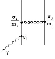
Figure 7: The two-quark gluon exchange current gives rise to a two-quark quadrupole operator as in Eq.(30) and a cubic quark mass dependence of SU(3) flavor symmetry breaking as in Eq.(32). The additional factor $1/m_{i}$ in Eq.(32) is due to the intermediate quark propagator between the photon-quark and gluon-quark vertices.

Flavor symmetry breaking is then characterized by the ratio $r=m_{u}/m_{s}$ of $u$ and $s$ quark masses, which is a known number. We use the same mass for $u$ and $d$ quarks to preserve the SU(2) isospin symmetry of the strong interaction, that is known to hold to a very good accuracy.

We emphasize that this treatment of SU(3) symmetry breaking is not exact. The GP method of including SU(3) symmetry breaking is to introduce additional operators and parameters, which guarantees that flavor symmetry breaking is incorporated to all orders Mor99a . There are then so many undetermined constants that the theory can no longer make predictions. We expect that our approximate treatment includes the most important physical effect.

Table 3: Two-quark ($B$) and three-quark ($C$) contributions to quadrupole moments of decuplet baryons in the SU(3) symmetry limit ($r=1$) and with broken flavor symmetry ($r\neq 1$). SU(3) flavor symmetry breaking is characterized by the ratio of u-quark and s-quark masses $r=m_{u}/m_{s}$.

	$Q(r=1)$	$Q(r\neq 1$
$\Delta^{-}$	$-4B-4C$	$-4B-4C$
$\Delta^{0}$	$0$	$0$
$\Delta^{+}$	$4B+4C$	$4B+4C$
$\Delta^{++}$	$8B+8C$	$8B+8C$
$\Sigma^{\ast-}$	$-4B-4C$	$-(4B+4C)(1+r+r^{2})/3$
$\Sigma^{\ast 0}$	$0$	$[2B(1+r-2r^{2})-2C(2-r-r^{2})]/3$
$\Sigma^{\ast+}$	$4B+4C$	$[4B(2+2r-r^{2})-4C(1-2r-2r^{2})]/3$
$\Xi^{\ast-}$	$-4B-4C$	$-(4B+4C)(r+r^{2}+r^{3})/3$
$\Xi^{\ast 0}$	$0$	$[4B(2r-r^{2}-r^{3})-4C(r+r^{2}-2r^{3})]/3$
$\Omega^{-}$	$-4B-4C$	$-(4B+4C)r^{3}$

Table 4: Two-quark ($B$) and three-quark ($C$) contributions to the octet-decuplet transition quadrupole moments in the SU(3) symmetry limit ($r=1$) and with broken flavor symmetry ($r\neq 1$). SU(3) flavor symmetry breaking is characterized by the ratio of u-quark and s-quark masses $r=m_{u}/m_{s}$.

	$Q(r=1)$	$Q(r\neq 1)$
$p\to\Delta^{+}$	$2\sqrt{2}(B-2C)$	$2\sqrt{2}\,(B-2C)$
$n\to\Delta^{0}$	$2\sqrt{2}(B-2C)$	$2\sqrt{2}\,(B-2C)$
$\Sigma^{-}\to\Sigma^{\ast-}$	$0$	$-\sqrt{2}\,(2B+2C)\,(2-r-r^{2})/3$
$\Sigma^{0}\to\Sigma^{\ast 0}$	$\sqrt{2}(B-2C)$	$\sqrt{2}[2B(2-r+2r^{2})-2C(4+r+r^{2})]/6$
$\Lambda^{0}\to\Sigma^{\ast 0}$	$\sqrt{6}(B-2C)$	$\sqrt{6}[2Br-2C(r+r^{2})]/2$
$\Sigma^{+}\to\Sigma^{\ast+}$	$2\sqrt{2}(B-2C)$	$2\sqrt{2}\,[B\,(4-2r+r^{2})-2C\,(1+r+r^{2})]/3$
$\Xi^{-}\to\Xi^{\ast-}$	$0$	$-\sqrt{2}\,(2B+2C)\,(r+r^{2}-2r^{3})/3$
$\Xi^{0}\to\Xi^{\ast 0}$	$2\sqrt{2}(B-2C)$	$\sqrt{2}[2B(2r-r^{2}+2r^{3})-2C(r+r^{2}+4r^{3})]/3$

V.3 Relations among quadrupole moments

Even though the SU(6) and SU(3) symmetries are broken, there exist –as a consequence of the underlying unitary symmetries— certain relations among the quadrupole moments. A relation is the stronger the weaker the assumptions required for its derivation. We were therefore interested in those relations that hold even when SU(3) symmetry breaking is included in the charge quadrupole operator. These are the ones, which are most likely satisfied in nature. The 18 quadrupole moments (10 diagonal decuplet and 8 decuplet-octet transition quadrupole moments) are expressed in terms of only two constants $B$ and $C$. Therefore, there must be 16 relations between them. Given the analytical expressions in Tables 3 and 4, it is straightforward to verify that the following relations hold

$$0 = Q_{\Delta^{-}}+Q_{\Delta^{+}},$$ (33a)

$$0 = Q_{\Delta^{0}},$$ (33b)

$$0 = 2\,Q_{\Delta^{-}}+Q_{\Delta^{++}},$$ (33c)

$$0 = Q_{\Sigma^{*-}}-2\,Q_{\Sigma^{*0}}+Q_{\Sigma^{*+}},$$ (33d)

$$0 = 3(Q_{\Xi^{*-}}-Q_{\Sigma^{*-}})-(Q_{\Omega^{-}}-Q_{\Delta^{-}}),$$ (33e)

$$0 = Q_{p\to\Delta^{+}}-\,Q_{n\to\Delta^{0}},$$ (33f)

$$0 = Q_{\Sigma^{-}\to\Sigma^{*-}}-2\,Q_{\Sigma^{0}\to\Sigma^{*0}}+Q_{\Sigma^{+}\to\Sigma^{*+}},$$ (33g)

$$0 = Q_{\Delta^{-}}-Q_{\Sigma^{*-}}-\sqrt{2}\,Q_{\Sigma^{-}\to\Sigma^{*-}},$$ (33h)

$$0 = Q_{\Delta^{+}}\!-\!Q_{\Sigma^{*+}}\!+\!\sqrt{2}Q_{p\to\Delta^{+}}\!-\!\sqrt{2}Q_{\Sigma^{+}\to\Sigma^{*+}},$$ (33i)

$$0 = Q_{\Sigma^{*0}}+Q_{\Xi^{*0}}$$ (33j)

$$- \!\!\!\frac{1}{\sqrt{2}}\left(Q_{\Sigma^{0}\to\Sigma^{*0}}\!-\!Q_{\Xi^{0}\to\Xi^{*0}}\!+\!\frac{1}{\sqrt{6}}Q_{\Lambda^{0}\to\Sigma^{*0}}\right)\!\!,$$

$$0 \!\!=\!\! Q_{\Sigma^{*-}}\!\!-\!Q_{\Xi^{*-}}\!\!-\!\!\frac{1}{\sqrt{2}}Q_{\Xi^{-}\!\to\!\Xi^{*-}}\!\!-\!\!\frac{1}{\sqrt{2}}Q_{\Sigma^{-}\!\to\!\Sigma^{*-}}\!.$$ (33k)

These eleven combinations of quadrupole moments do not depend on the flavor symmetry breaking parameter $r$. In fact, Eqs.(33a-33d) are already a consequence of the assumed SU(2) isospin symmetry of the strong interaction, and hold irrespective of the order of SU(3) symmetry breaking. Eq.(33e) is the quadrupole moment counterpart of the “equal spacing rule” for decuplet masses.

There are also five $r$-dependent relations which can be chosen as

$$0 = \frac{1}{3}(1+r+r^{2})Q_{\Delta^{+}}+Q_{\Sigma^{*-}},$$ (34a)

$$0 = (r-r^{2})\,Q_{\Delta^{+}}-\sqrt{2}(2+r^{2})Q_{p\to\Delta^{+}}$$ (34b)

$$+ 6\sqrt{2}Q_{\Sigma^{0}\to\Sigma^{*0}},$$

$$0 = r\,Q_{\Sigma^{*-}}-Q_{\Xi^{*-}},$$ (34c)

$$0 = (r-r^{2})Q_{\Delta^{+}}+\sqrt{2}(r+2r^{3})\,Q_{p\to\Delta^{+}}$$ (34d)

$$- 3\sqrt{2}\,Q_{\Xi^{0}\to\Xi^{*0}},$$

$$0 = r^{3}\,Q_{\Delta^{-}}-Q_{\Omega^{-}}.$$ (34e)

Other combinations of the expressions in Tables 3 and 4 can be written down if desirable. With the help of these relations the experimentally inaccessible quadrupole moments can be obtained from those that can be measured. Quadrupole moments of decuplet baryons are difficult to measure due to their short lifetime with the exception of the $\Omega^{-}$. It is planned to measure the quadrupole moment of the relatively long-lived $\Omega^{-}$ baryon at FAIR in Darmstadt Poc17 .

Table 5: Numerical values for the quadrupole moments of decuplet baryons in units of [fm²] according to the analytic expressions in Table 3 with $B=r_{n}^{2}/4$ and $C=0$. The experimental neutron charge radius Kop95 , $r_{n}^{2}=-0.113(3)$ fm², and the SU(3) symmetry breaking parameter hen00a , $r=0.6$, are used as input values.

	${Q}(r=1)$	$Q(r=0.6)$
$\Delta^{-}$	$0.113$	0.113
$\Delta^{0}$	0	0
$\Delta^{+}$	$-0.113$	-0.113
$\Delta^{++}$	$-0.226$	-0.226
$\Sigma^{\ast-}$	$0.113$	0.074
$\Sigma^{\ast 0}$	0	-0.017
$\Sigma^{\ast+}$	$-0.113$	-0.107
$\Xi^{\ast-}$	$0.113$	0.044
$\Xi^{\ast 0}$	0	-0.023
$\Omega^{-}$	$0.113$	0.024

Table 6: Numerical values for the octet-decuplet transition quadrupole moments in units of [fm²] according to the analytic expressions in Table 4.

	${Q}(r=1)$	$Q(r=0.6)$
$p\rightarrow\Delta^{+}$	$-0.080$	-0.080
$n\rightarrow\Delta^{0}$	$-0.080$	-0.080
$\Sigma^{-}\rightarrow\Sigma^{\ast-}$	$0$	0.028
$\Sigma^{0}\rightarrow\Sigma^{\ast 0}$	$-0.040$	-0.028
$\Lambda^{0}\rightarrow\Sigma^{\ast 0}$	$-0.069$	-0.042
$\Sigma^{+}\rightarrow\Sigma^{\ast+}$	$-0.080$	-0.084
$\Xi^{-}\rightarrow\Xi^{\ast-}$	0	0.014
$\Xi^{0}\rightarrow\Xi^{\ast 0}$	$-0.080$	-0.034

V.4 Numerical results

Numerical values are listed in Tables 5 and 6 for the cases without ($r=1$) and with ($r=0.6$) flavor symmetry breaking. The electric quadrupole moments of the charged baryons are of the same order of magnitude as $r_{n}^{2}$, while those of the neutral baryons are considerably smaller. Updated numerical results including the three-quark terms have been given in Ref. Buc07 .

Electric quadrupole moments and their generalization to quadrupole form factors have been the focus of numerous works But94 ; Leb95 ; Oh95 ; Dah13 ; Kri91 ; Buc04 ; Pas07a ; Ram16 and several reviews Pas07 ; Ber07 ; Tia07 ; Tia11 ; Azn11 .

VI Magnetic octupole moments of baryons

While there is a large body of literature on baryon magnetic dipole moments, there are only few works that deal with the next higher multipole moments, that is the magnetic octupole moments $\Omega$ of decuplet baryons Gia90 ; Hen08 ; Ram09 ; Ali09 . Presently, relatively little is known concerning the sign and the size of these moments. This information is needed to reveal further details of the current distribution in baryons beyond those available from the magnetic dipole moment kot02 .

The magnetic octupole moment operator $\Omega$ usually given in units $[{\rm fm}^{2}\,\mu_{N}]$ and normalized as in Ref. Don84 can be written as

$$\Omega_{0} = \frac{3}{8}\int\!dr^{3}(3z^{2}-r^{2})\,({\bf r}\times{\bf J}({\bf r}))_{z},$$ (35)

where ${\bf J}({\bf r})$ is the spatial current density and $\mu_{N}$ the nuclear magneton. This definition is analogous to the one for the charge quadrupole moment hen00b if the magnetic moment density $({\bf r}\times{\bf J}({\bf r}))_{z}$ is replaced by the charge density $\rho({\bf r})$. Again, one has to distinguish between the spectroscopic (laboratory frame) and intrinsic (body-fixed frame). Thus, the magnetic octupole moment measures the deviation of the spatial magnetic moment distribution from spherical symmetry. More specifically, for a prolate (cigar-shaped) magnetic moment distribution $\Omega_{0}>0$, while for an oblate (pancake-shaped) magnetic moment distribution $\Omega_{0}<0$. We also see from Eq.(35) that the typical size of a magnetic octupole moment is

$$\Omega_{0}\simeq r^{2}\,\mu$$ (36)

where $\mu$ is the magnetic moment and $r^{2}$ a size parameter related to the quadrupole moment of the system. Although the nucleon cannot have a spectroscopic octupole moment, due to angular momentum selection rules, it may have an intrinsic octupole moment, if its magnetic moment distribution deviates from spherical symmetry Buc18 .

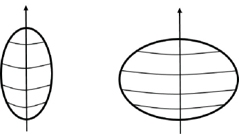
Figure 8: Magnetic octupole moment of the current distribution. Left: Prolate current distribution with an intrinsic octupole moment $\Omega_{0}>0$. Right: Oblate current distribution with an intrinsic octupole moment $\Omega_{0}<0$. For further details see Buc18 ).

To calculate the spectroscopic octupole moments of decuplet baryons we had to construct an octupole moment operator ${\tilde{\Omega}}$ in spin-flavor space. We knew that we needed a tensor of rank 3 in spin space, which must involve the Pauli spin matrices of three different quarks comment0 . This could be done by considering a three-body quadrupole moment operator multiplied by the spin of the third quark,

$${\tilde{\Omega}}_{[3]} = C\sum_{i\neq j\neq k}^{3}e_{k}\left(3\sigma_{i\,z}\sigma_{j\,z}-\mbox{\boldmath$\sigma$}_{i}\cdot\mbox{\boldmath$\sigma$}_{j}\right)\mbox{\boldmath$\sigma$}_{k},$$ (37)

where $C$ is a constant and $e_{k}=(1+3\tau_{k\,z})/6$ is the charge of the k-th quark. The $z$-component of the Pauli spin (isospin) matrix $\mbox{\boldmath$\sigma$}_{i}$ ($\mbox{\boldmath$\tau$}_{i}$) is denoted by $\sigma_{i\,z}$ ($\tau_{i\,z}$). Alternatively, it could be built by replacing $e_{k}$ in Eq.(refpara2) by $e_{i}$, i.e. from a two-quark quadrupole operator. We soon realized that both operator structures lead to the same results. In addition, we found that from the point of view of broken SU(6) spin-flavor symmetry Gur64 , there is a unique octupole moment operator comment22 .

The spectroscopic magnetic octupole moments $\Omega_{B^{*}}$ were then obtained by sandwiching the operator in Eq.(37)between the three-quark spin-flavor wave functions $|W_{B^{*}}\rangle$. For example, for $\Delta(1232)$ baryons we obtained

$$\Omega_{\Delta} = \langle W_{\Delta}|{\tilde{\Omega}}_{[3]}|W_{\Delta}\rangle=4\,C\,q_{\Delta},$$ (38)

where $q_{\Delta}$ is the $\Delta$ charge. Similarly, the magnetic octupole moments for the other decuplet baryons were calculated. In this way Morpurgo’s method yields an efficient parameterization of baryon octupole moments in terms of just one unknown parameter $C$.

In the second column of Table 7 we show our results for the decuplet octupole moments expressed in terms of the GP constant $C$ assuming that SU(3) flavor symmetry is only broken by the electric charge operator as in Eq.(37). We observe that in this limit the spectroscopic magnetic octupole moments are proportional to the baryon charge.

Table 7: Magnetic octupole moments of decuplet baryons. Second column: SU(3) flavor symmetry limit ($r=1$). Third column: with flavor symmetry breaking ($r\neq 1$).

	$\Omega_{B^{*}}(r=1)$	$\Omega_{B^{*}}(r\neq 1)$
$\Delta^{-}$	$-4C$	$-4C$
$\Delta^{0}$	0	0
$\Delta^{+}$	$4C$	$4C$
$\Delta^{++}$	$8C$	$8C$
$\Sigma^{\ast-}$	$-4C$	$-4C\,(1+r+r^{2})/3$
$\Sigma^{\ast 0}$	$0$	$-2C\,(2-r-r^{2})/3$
$\Sigma^{\ast+}$	$4C$	$-4C\,(1-2r-2r^{2})/3$
$\Xi^{\ast-}$	$-4C$	$-4C\,(r+r^{2}+r^{3})/3$
$\Xi^{\ast 0}$	$0$	$-4C\,(r+r^{2}-2r^{3})/3$
$\Omega^{-}$	$-4C$	$-4C\,r^{3}$

To estimate the degree of SU(3) flavor symmetry breaking beyond first order, we replaced the spin-spin terms in Eq.(37) by expressions with a cubic quark mass dependence as in Eq.(32). This leads to analytic expressions for the magnetic octupole moments $\Omega_{B^{*}}$ containing terms up to third order in $r$ as shown in the third column of Table 7.

Because the 10 diagonal octupole moments can be expressed in terms of only one constant $C$, there must be 9 relations between them. Given the analytical expressions in Table 7 it is straightforward to verify that the following relations hold

$$0 = \Omega_{\Delta^{-}}+\Omega_{\Delta^{+}},$$ (39a)

$$0 = \Omega_{\Delta^{0}},$$ (39b)

$$0 = 2\,\Omega_{\Delta^{-}}+\Omega_{\Delta^{++}},$$ (39c)

$$0 = \Omega_{\Sigma^{*-}}-2\,\Omega_{\Sigma^{*0}}+\Omega_{\Sigma^{*+}},$$ (39d)

$$0 = 3(\Omega_{\Xi^{*-}}-\Omega_{\Sigma^{*-}})-(\Omega_{\Omega^{-}}-\Omega_{\Delta^{-}})$$ (39e)

$$0 = (\Omega_{\Xi^{*0}}+2\,\Omega_{\Xi^{*-}})+(\Omega_{\Sigma^{*+}}-\Omega_{\Sigma^{*-}})$$ (39f)

$$0 = \frac{1}{3}(1+r+r^{2})\Omega_{\Delta^{+}}+\Omega_{\Sigma^{*-}},$$ (39g)

$$0 = r\,\Omega_{\Sigma^{*-}}-\Omega_{\Xi^{*-}},$$ (39h)

$$0 = r^{3}\,\Omega_{\Delta^{-}}-\Omega_{\Omega^{-}}.$$ (39i)

The first six relations do not depend on the flavor symmetry breaking parameter $r$. In fact, Eqs.(39a-39d) are already a consequence of the assumed SU(2) isospin symmetry of strong interactions. Eq.(39e) is the octupole moment counterpart of the “equal spacing rule” for decuplet masses. Other combinations of the expressions in Table 7 can be written down if desirable.

To obtain an estimate for $\Omega_{\Delta^{+}}$ we use the pion cloud model hen00b where the $\Delta^{+}$ wave function without bare $\Delta$ and for maximal spin projection $J_{z}=1/2$ is writtten as

$$|\Delta^{+}J_{z}=\frac{3}{2}\rangle=\beta^{\prime}\,\Bigl{(}\sqrt{\frac{1}{3}}\,|n^{\prime}\,\pi^{+}\rangle+\sqrt{\frac{2}{3}}\,|p^{\prime}\,\pi^{0}\rangle\Bigr{)}|\uparrow\,Y^{1}_{1}\rangle.$$ (40)

In this model the magnetic octupole moment operator is a product of a quadrupole operator in pion variables and a magnetic moment operator in nucleon variables

$$\Omega_{\pi N}=\sqrt{\frac{16\pi}{5}}\,r_{\pi}^{2}\,Y^{2}_{0}({\bf r}_{\pi})\,\,\mu_{N}\,\tau_{z}^{N}\,\sigma_{z}^{N}.$$ (41)

Here, the spin-isospin structure of $\Omega_{\pi N}$ is infered from the $\gamma\pi N$ and $\gamma\pi$ currents of the static pion-nucleon model Hen62 .

With Eq.(40) and Eq.(41) the $\Delta^{+}$ magnetic octupole moment was readily calculated Hen08

$$\Omega_{\Delta^{+}}=-{2\over 15}\,{\beta^{\prime}}^{2}\,r_{\pi}^{2}\ \mu_{N}=Q_{\Delta^{+}}\,\mu_{N}=r_{n}^{2}\,\mu_{N},$$ (42)

where $Q_{\Delta^{+}}$ is the $\Delta^{+}$ quadrupole moment and $r_{n}^{2}$ the neutron charge radius. With the experimental value of the latter and $\mu_{N}$ expressed in $[{\rm fm}]$ we obtained $\Omega_{\Delta^{+}}=-0.012\,\,{\rm fm^{3}}$. The negative value of $\Omega$ implies that the magnetic moment distribution in the $\Delta^{+}$ is oblate and hence has the same geometric shape as the charge distribution. Numerical values for other baryon octupole moments can now be obtained using Eq.(38) and the expressions in Table 7. These are listed in Table 8.

Table 8: Numerical values for magnetic octupole moments of decuplet baryons in units [fm³] using Table 7 with $C=-0.003$. Second column: SU(3) flavor symmetry limit ($r=1$). Third column: with SU(3) flavor symmetry breaking ($r=0.6$).

	$\Omega_{B^{*}}(r=1)$	$\Omega_{B^{*}}(r=0.6)$
$\Delta^{-}$	0.012	0.012
$\Delta^{0}$	0	0
$\Delta^{+}$	-0.012	-0.012
$\Delta^{++}$	-0.024	-0.024
$\Sigma^{\ast-}$	0.012	0.008
$\Sigma^{\ast 0}$	0	0.002
$\Sigma^{\ast+}$	-0.012	-0.004
$\Xi^{\ast-}$	0.012	0.005
$\Xi^{\ast 0}$	0	0.002
$\Omega^{-}$	0.012	0.003

To draw a first conclusion concerning the spatial shape of the magnetic moment distribution in baryons we estimated the spectroscopic magnetic octupole moment of the $\Delta^{+}$ in the pion cloud model. We found that the latter can be expressed as the product of the $\Delta^{+}$ quadrupole moment and the nuclear magneton. This means that the magnetic moment distribution in the $\Delta^{+}$ is oblate and hence has the same geometric shape as the charge distribution. Recently, an attempt has been made to extract the intrinsic octupole moment of the proton from these results Buc18 .

VII Spin and orbital angular momentum of ground state baryons

The question how the proton spin is made up from the quark spin $\Sigma$, quark orbital angular momentum $L_{q}$, gluon spin $S_{g}$, and gluon orbital angular momentum $L_{g}$

$$J=\frac{1}{2}\Sigma+L_{q}+S_{g}+L_{g}$$ (43)

is one of the central issues in nucleon structure physics seh74 ; ji97 . In the constituent quark model with only one-quark operators, also called additive quark model, one obtains $J=\Sigma/2=1/2$, i.e., the proton spin is the sum of the constituent quark spins and nothing else. However, experimentally it is known that only about 1/3 of the proton spin comes from quarks aid12 . The disagreement between the additive quark model result and experiment came as a surprise because the same model accurately described the related proton and neutron magnetic moments. We showed that the failure of the additive quark model to describe the quark contribution to proton spin correctly is due to its neglect of three-quark terms in the axial current Hen11 .

The first step is to realize Gur64 that a general SU(6) spin-flavor operator ${\tilde{\Omega}}^{R}$ acting on the ${\bf 56}$ dimensional baryon ground state supermultiplet must transform according to one of the irreducible representations $R$ contained in the direct product $\bar{{\bf 56}}\times{\bf 56}={\bf 1}+{\bf 35}+{\bf 405}+{\bf 2695}.$ The ${\bf 1}$ dimensional representation (rep) corresponds to an SU(6) symmetric operator, while the ${\bf 35}$, ${\bf 405}$, and ${\bf 2695}$ dimensional reps characterize respectively, first, second, and third order SU(6) symmetry breaking. Therefore, a general SU(6) symmetry breaking operator for ground state baryons has the form

$${\tilde{\Omega}}={\tilde{\Omega}}^{\bf 35}+{\tilde{\Omega}}^{\bf 405}+{\tilde{\Omega}}^{\bf 2695}.$$ (44)

The second step is to decompose each SU(6) tensor ${\tilde{\Omega}}^{R}$ in Eq.(44) into SU(3)${}_{F}\times$SU(2)_J subtensors ${\tilde{\Omega}}^{R}_{(F,2J+1)}$, where $F$ and $2J+1$ are the dimensionalities of the flavor and spin reps. One finds  Hen11 ; Beg64a that a flavor singlet $(F=1)$ axial vector $(J=1)$ operator ${\tilde{\Omega}}^{R}_{({\bf 1},{\bf 3})}$ needed to describe baryon spin, is contained only in the $R={\bf 35}$ and $R={\bf 2695}$ dimensional reps of SU(6).

The third step is to construct quark operators transforming as the SU(6) tensor ${\tilde{\Omega}}^{R}_{({\bf 1},{\bf 3})}$. In terms of quarks, the SU(6) tensors on the right-hand side of Eq.(44) are represented respectively by one-, two-, and three-quark operators Leb95 . We found the following uniquely determined one-quark ${\bf A}_{[1]}$ and three-quark ${\bf A}_{[3]}$ flavor singlet axial currents Hen11

$${\tilde{\Omega}}^{\bf 35}_{({\bf 1},{\bf 3})} = {\bf A}_{[1]}=A\,\sum_{i=1}^{3}\ {\hbox{$\sigma$}\hbox to0.0pt{\hss\hbox{$\sigma$}\hskip 0.39993pt}\hbox to0.0pt{\hss\lower 0.17218pt\hbox{\hbox{$\sigma$}\hbox to0.0pt{\hss\hbox{$\sigma$}\hskip 0.39993pt}}}}_{i},$$

$${\tilde{\Omega}}^{\bf 2695}_{({\bf 1},{\bf 3})} = {\bf A}_{[3]}=C\,\sum_{i\neq j\neq k}^{3}\ {\hbox{$\sigma$}\hbox to0.0pt{\hss\hbox{$\sigma$}\hskip 0.39993pt}\hbox to0.0pt{\hss\lower 0.17218pt\hbox{\hbox{$\sigma$}\hbox to0.0pt{\hss\hbox{$\sigma$}\hskip 0.39993pt}}}}_{i}\cdot{\hbox{$\sigma$}\hbox to0.0pt{\hss\hbox{$\sigma$}\hskip 0.39993pt}\hbox to0.0pt{\hss\lower 0.17218pt\hbox{\hbox{$\sigma$}\hbox to0.0pt{\hss\hbox{$\sigma$}\hskip 0.39993pt}}}}_{j}\ {\hbox{$\sigma$}\hbox to0.0pt{\hss\hbox{$\sigma$}\hskip 0.39993pt}\hbox to0.0pt{\hss\lower 0.17218pt\hbox{\hbox{$\sigma$}\hbox to0.0pt{\hss\hbox{$\sigma$}\hskip 0.39993pt}}}}_{k},$$ (45)

where $\hbox{$\sigma$}\hbox to0.0pt{\hss\hbox{$\sigma$}\hskip 0.39993pt}\hbox to0.0pt{\hss\lower 0.17218pt\hbox{\hbox{$\sigma$}\hbox to0.0pt{\hss\hbox{$\sigma$}\hskip 0.39993pt}}}_{i}$ is the Pauli spin matrix of quark $i$. The constants $A$ and $C$ are to be determined from experiment. The most general flavor singlet axial current compatible with broken SU(6) symmetry is then

$${\bf A}={\bf{A}}_{[1]}+{\bf{A}}_{[3]}=A\,\sum_{i=1}^{3}\ {\hbox{$\sigma$}\hbox to0.0pt{\hss\hbox{$\sigma$}\hskip 0.39993pt}\hbox to0.0pt{\hss\lower 0.17218pt\hbox{\hbox{$\sigma$}\hbox to0.0pt{\hss\hbox{$\sigma$}\hskip 0.39993pt}}}}_{i}+C\,\sum_{i\neq j\neq k}^{3}\ {\hbox{$\sigma$}\hbox to0.0pt{\hss\hbox{$\sigma$}\hskip 0.39993pt}\hbox to0.0pt{\hss\lower 0.17218pt\hbox{\hbox{$\sigma$}\hbox to0.0pt{\hss\hbox{$\sigma$}\hskip 0.39993pt}}}}_{i}\cdot{\hbox{$\sigma$}\hbox to0.0pt{\hss\hbox{$\sigma$}\hskip 0.39993pt}\hbox to0.0pt{\hss\lower 0.17218pt\hbox{\hbox{$\sigma$}\hbox to0.0pt{\hss\hbox{$\sigma$}\hskip 0.39993pt}}}}_{j}\ {\hbox{$\sigma$}\hbox to0.0pt{\hss\hbox{$\sigma$}\hskip 0.39993pt}\hbox to0.0pt{\hss\lower 0.17218pt\hbox{\hbox{$\sigma$}\hbox to0.0pt{\hss\hbox{$\sigma$}\hskip 0.39993pt}}}}_{k}.$$ (46)

The additive quark model corresponds to $C=0$ and $A=1$. The three-quark operators are an effective description of quark-antiquark and gluon degrees of freedom. Prior to our investigation, the role of two-body gluon exchange currents was studied in the nucleon spin problem Bar06 ; tho09 in more elaborate models but with similar results for the nucleon. The relation between these approaches has not yet been clarified.

VII.1 Quark spin contribution to baryon spin

By sandwiching the flavor singlet axial current ${\bf A}$ of Eq.(46) between standard SU(6) baryon wave functions Clo we obtained for the quark spin contribution to the spin of octet and decuplet baryons Hen11

$$\Sigma_{1}: = \langle B_{8}\uparrow|{\bf A}_{z}|B_{8}\uparrow\rangle=A-10\,C,$$

$$\Sigma_{3}: = \langle B_{10}\uparrow|{\bf A}_{z}|B_{10}\uparrow\rangle=3\,A+6\,C,$$ (47)

where $B_{8}$ ($B_{10}$) stands for any member of the baryon flavor octet (decuplet). Here, $\Sigma_{1}$ ($\Sigma_{3}$) is twice the quark spin contribution to octet (decuplet) baryon spin. Our theory predicts the same quark contribution to baryon spin for all members of a given flavor multiplet, because the operator in Eq.(46) is by construction a flavor singlet that does not break SU(3) flavor symmetry. On the other hand, SU(6) spin-flavor symmetry is broken as reflected by the different expressions for flavor octet and decuplet baryons.

We then constructed from the operators in Eq.(46) one-body ${\bf A}^{q}_{[1]\,z}$ and three-body ${\bf A}^{q}_{[3]\,z}$ operators of flavor $q$ acting only on $u$ quarks and $d$ quarks Hen11

$${\bf A}_{z}^{u} = A\sum_{i=1}^{3}\hbox{$\sigma$}\hbox to0.0pt{\hss\hbox{$\sigma$}\hskip 0.39993pt}\hbox to0.0pt{\hss\lower 0.17218pt\hbox{\hbox{$\sigma$}\hbox to0.0pt{\hss\hbox{$\sigma$}\hskip 0.39993pt}}}^{u}_{i\,z}+2C\sum_{i\neq j\neq k}^{3}{\hbox{$\sigma$}\hbox to0.0pt{\hss\hbox{$\sigma$}\hskip 0.39993pt}\hbox to0.0pt{\hss\lower 0.17218pt\hbox{\hbox{$\sigma$}\hbox to0.0pt{\hss\hbox{$\sigma$}\hskip 0.39993pt}}}}^{u}_{i}\cdot{\hbox{$\sigma$}\hbox to0.0pt{\hss\hbox{$\sigma$}\hskip 0.39993pt}\hbox to0.0pt{\hss\lower 0.17218pt\hbox{\hbox{$\sigma$}\hbox to0.0pt{\hss\hbox{$\sigma$}\hskip 0.39993pt}}}}^{d}_{j}\ {\hbox{$\sigma$}\hbox to0.0pt{\hss\hbox{$\sigma$}\hskip 0.39993pt}\hbox to0.0pt{\hss\lower 0.17218pt\hbox{\hbox{$\sigma$}\hbox to0.0pt{\hss\hbox{$\sigma$}\hskip 0.39993pt}}}}^{u}_{k\,z},$$

$${\bf A}_{z}^{d} = A\sum_{i=1}^{3}\hbox{$\sigma$}\hbox to0.0pt{\hss\hbox{$\sigma$}\hskip 0.39993pt}\hbox to0.0pt{\hss\lower 0.17218pt\hbox{\hbox{$\sigma$}\hbox to0.0pt{\hss\hbox{$\sigma$}\hskip 0.39993pt}}}^{d}_{i\,z}+C\sum_{i\neq j\neq k}^{3}{\hbox{$\sigma$}\hbox to0.0pt{\hss\hbox{$\sigma$}\hskip 0.39993pt}\hbox to0.0pt{\hss\lower 0.17218pt\hbox{\hbox{$\sigma$}\hbox to0.0pt{\hss\hbox{$\sigma$}\hskip 0.39993pt}}}}^{u}_{i}\cdot{\hbox{$\sigma$}\hbox to0.0pt{\hss\hbox{$\sigma$}\hskip 0.39993pt}\hbox to0.0pt{\hss\lower 0.17218pt\hbox{\hbox{$\sigma$}\hbox to0.0pt{\hss\hbox{$\sigma$}\hskip 0.39993pt}}}}^{u}_{j}\ {\hbox{$\sigma$}\hbox to0.0pt{\hss\hbox{$\sigma$}\hskip 0.39993pt}\hbox to0.0pt{\hss\lower 0.17218pt\hbox{\hbox{$\sigma$}\hbox to0.0pt{\hss\hbox{$\sigma$}\hskip 0.39993pt}}}}^{d}_{k\,z}.$$ (48)

For the $u$ and $d$ quark contributions to the spin of the proton we obtained

$$\Delta u = \langle p\uparrow|\,{\bf A}_{[1]\,z}^{u}+{\bf A}_{[3]\,z}^{u}|p\uparrow\rangle=\phantom{-}\frac{4}{3}\,A-\frac{28}{3}\,C,$$

$$\Delta d = \langle p\uparrow|\,{\bf A}_{[1]\,z}^{d}+{\bf A}_{[3]\,z}^{d}|p\uparrow\rangle=-\frac{1}{3}\,A-\frac{2}{3}\,C.$$ (49)

These theoretical results were compared with the combined deep inelastic scattering and hyperon $\beta$-decay experimental data, from which the following quark spin contributions to the proton spin were extracted aid12 $\Delta u=\hskip 9.95863pt0.84\pm 0.03,\hskip 14.22636pt\Delta d=-0.43\pm 0.03,\hskip 14.22636pt\Delta s=-0.08\pm 0.03.$ The sum of these spin fractions $\Sigma_{1_{exp}}=\Delta u+\Delta d+\Delta s=0.33(08)$ is considerably smaller than expected from the additive quark model, which gives $\Sigma_{1}=1$.

Solving Eq.(VII.1) for $A$ and $C$ fixes the constants $A$ and $C$ as

$$A=\phantom{-}\frac{1}{6}\,\,\Delta u-\frac{7}{3}\,\Delta d,\qquad C=-\frac{1}{12}\,\Delta u-\frac{1}{3}\,\Delta d.$$ (50)

Inserting the experimental results for $\Delta u$ and $\Delta d$ we obtain $A=1.143(70)$ and $C=0.073(10)$ and from Eq.(VII.1)

$$\Sigma_{1} = A-10\,C=1.14-0.73=0.41(12),$$

$$\Sigma_{3} = 3\,A+6\,C=3.42+0.45=3.87(22)$$ (51)

compared to the experimental result $\Sigma_{1_{exp}}=0.33(08)$. For octet baryons, the three-quark term is of the same importance as the one-quark term because of the factor 10 multiplying $C$. It is interesting that for decuplet baryons, quark spins add up to 1.3 times the additive quark model value $\Sigma_{3}=3$.

VII.2 Quark orbital angular momentum contribution to baryon spin

We then applied Hen14 the spin-flavor operator analysis of Sect. VII.1 to quark orbital angular momentum $L_{z}$ using the general operator of Eq.(46) for $L_{z}$ with new constants $A^{\prime}$ and $C^{\prime}$

$$L_{z}(8) = \langle B_{8}\uparrow|{L}_{z}|B_{8}\uparrow\rangle=\frac{1}{2}\left(A^{\prime}-10\,C^{\prime}\right),$$

$$L_{z}(10) = \langle B_{10}\uparrow|{L}_{z}|B_{10}\uparrow\rangle=\frac{1}{2}\left(3\,A^{\prime}+6\,C^{\prime}\right).$$ (52)

Assuming that the gluon total angular momentum $S_{g}+L_{g}\approx 0$ is small aid12 we obtained from Eq.(43)

$$L_{z}(8) = \frac{1}{2}-\frac{1}{2}\Sigma_{1}=0.30,$$

$$L_{z}(10) = \frac{3}{2}-\frac{1}{2}\Sigma_{3}=-0.44.$$ (53)

Eq.(VII.2) and Eq.(VII.2) yielded for the parameters $A^{\prime}=1-A=-0.143$ and $C^{\prime}=-C=-0.073$.

Next, we calculated the orbital angular momentum carried by $u$ and $d$ quarks in the proton in analogy to Eq.(VII.1)

$$L_{z}^{u}(p) = \frac{1}{2}\left(\frac{4}{3}\,A^{\prime}-\frac{28}{3}\,C^{\prime}\right)=0.25,$$

$$L_{z}^{d}(p) = \frac{1}{2}\left(-\frac{1}{3}\,A^{\prime}-\frac{2}{3}\,C^{\prime}\right)=0.05.$$ (54)

For the total angular momentum carried by quarks we got $J^{u}(p)=\frac{1}{2}\Delta u+L_{z}^{u}(p)=0.42+0.25=0.67$ and $J^{d}(p)=\frac{1}{2}\Delta d+L_{z}^{d}(p)=-0.22+0.05=-0.17$. Our results for $J^{u}(p)$ and $J^{d}(p)$ are consistent with those of Thomas tho09 who finds $J^{u}(p)=0.67$ and $J^{d}(p)=-0.17$ at the low energy (model) scale. Applying the $u$ and $d$ quark operators in Eq.(VII.1) to the $\Delta^{+}$ state we obtain

$$L_{z}^{u}(\Delta^{+}) = \frac{1}{2}\left(2\,A^{\prime}+4\,C^{\prime}\right)=-0.29,$$

$$L_{z}^{d}(\Delta^{+}) = \frac{1}{2}\left(A^{\prime}+2\,C^{\prime}\right)=-0.15.$$ (55)

We suggested an interpretation of Eq.(VII.2) and Eq.(VII.2) in terms of the geometric shapes of these baryons as depicted in Fig. 9. Previously, by studying the electromagnetic $p\to\Delta^{+}$ transition in various baryon structure models, we have found that the proton has a positive intrinsic quadrupole moment $Q_{0}(p)$ corresponding to a prolate intrinsic charge distribution whereas the $\Delta^{+}$ has a negative intrinsic quadrupole moment of similar magnitude $Q_{0}(\Delta^{+})\approx-Q_{0}(p)$ corresponding to an oblate charge distribution hen00b . This appears to be consistent with our findings for the quark orbital angular momenta $L^{u}_{z}$ and $L^{d}_{z}$ in both systems as qualitatively shown in Fig. 9.

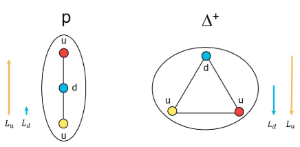
Figure 9: Qualitative picture of the $u$ and $d$ quark distributions in the proton (left) and $\Delta^{+}$ (right). In the proton, most of the quark orbital angular momentum is carried by the $u$ quarks and relatively little by the $d$ quarks. This is consistent with a linear (prolate or cigar-shaped) quark distribution with the $u$ quarks at the periphery and the $d$ quark near the origin. In contrast, in the $\Delta^{+}$, the $u$ quark orbital angular momentum is just twice that of the $d$ quark. This is consistent with a planar (oblate or pancake-shaped) quark distribution, in which each quark has the same distance from the origin.

In summary, using a broken spin-flavor symmetry based parametrization of QCD, we calculated the quark spin and orbital angular momentum contributions to total baryon spin for the octet and for the first time also for the decuplet. For flavor octet baryons, we demonstrated that three-quark operators reduce the standard quark model prediction based on one-quark operators from $\Sigma_{1}=1$ to $\Sigma_{1}=0.41(12)$ in agreement with the experimental result. On the other hand, in the case of flavor decuplet baryons, three-quark operators enhance the contribution of one quark operators from $\Sigma_{3}=3$ to $\Sigma_{3}=3.87(22)$.

Assuming that the gluon contribution to baryon spin is small, we suggested a qualitative interpretation of the positive and large $u$ quark and small $d$ quark orbital angular momenta in the proton in terms of a prolate quark distribution corresponding to a positive intrinsic quadrupole moment. In the case of the $\Delta^{+}$, $u$ and $d$ quarks have negative orbital angular momenta of the same magnitude corresponding to an oblate quark distribution giving rise to a negative intrinsic quadrupole moment.

Figure 10: Ernest Mark Henley (1924-2017).

VIII Epilogue

The last time I saw Ernest was in Seattle in the summer of 2013. We discussed the connection between quark orbital angular momentum and the nonsphericity of the nucleon within the context of a harmonic oscillator quark model. Ernest was in good health and he told me that he was still commuting to his office by bike but that his wife did not approve.

Looking back, I am very proud to have had the honour of working with Ernest Henley. He was a very good scientist with a unique gift for cutting through formalism and getting to the heart of the matter. His textbooks ”Subatomic physics” Fra74 and the more advanced ”Nuclear and particle physics” Fra75 are masterpieces of clarity and pedagogy. Ernest Henley will always be a role model, not only as an ingenious physicist but also as a human being. He will be missed very much by everybody who had the good fortune to know him.

References

- (1) H. Frauenfelder and E. M. Henley, Subatomic Physics (Prentice-Hall, Englewood Cliffs, 1974).
- (2) A. Buchmann, W. Leidemann, and H. Arenhövel, Nucl. Phys. A443, 726 (1985).
- (3) A. J. Buchmann, E. Hernández, and A. Faessler, Phys. Rev. C55, 448 (1997); A. J. Buchmann, E. Hernández, U. Meyer, and A. Faessler, Phys. Rev. C58, 2478 (1998).
- (4) G. Dillon and G. Morpurgo, Phys. Lett. B448, 107 (1999).
- (5) G. Morpurgo, Phys. Rev. D40, 2997 (1989); Phys. Rev. D40, 3111 (1989).
- (6) G. Morpurgo, Phys. Rev. Lett. 68, 139 (1992); Phys. Rev. D46, 4068 (1992).
- (7) A. J. Buchmann and E. M. Henley, Phys. Lett. B484, 255 (2000), AIP Conference Proceedings 539, 148 (2000).
- (8) A. J. Buchmann and E. M. Henley, Phys. Rev. C63, 015202, (2000).
- (9) A.J. Buchmann and E.M. Henley, Phys. Rev. D65, 073017 (2002).
- (10) A. J. Buchmann, E. M. Henley, Eur. Phys. J. A35, 267 (2008).
- (11) A. J. Buchmann, E. M. Henley, Phys. Rev. D83, 096011 (2011).
- (12) A. J. Buchmann, E. M. Henley, Few-Body Syst. 55, 749 (2014).
- (13) G. Dillon and G. Morpurgo, Phys. Rev. D53, 3754 (1996).
- (14) G. Dillon and G. Morpurgo, Phys. Lett. B459, 321 (1999); Z. Phys. C73, 547 (1997).
- (15) D. B. Lichtenberg, Unitary Symmetry and Elementary Particles, Academic Press, New York, 1978; F. E. Close, An introduction to Quarks and Partons, Academic Press, London, 1979.
- (16) R. Dashen, E. Jenkins, and A. V. Manohar, Phys. Rev. D49, 4713 (1994).
- (17) A. J. Buchmann and R. F. Lebed, Phys. Rev. D62, 096005 (2000), Phys. Rev. D67, 016002 (2003).
- (18) A. J. Buchmann, J. A. Hester, and R. F. Lebed, Phys. Rev. D66, 056002 (2002)
- (19) A. J. Buchmann and S. Moszkowski, Phys. Rev. C87,028203 (2013).
- (20) G. E. Brown and W. Weise, Phys. Rep. C22, 279 (1975).
- (21) V. Gupta and V. Singh, Phys. Rev. 135, B1442 (1964); C. Becchi, E. Eberle, and G. Morpurgo, Phys. Rev. 136, B808 (1964).
- (22) A. Bohr and B. Mottelson, Nuclear Structure II, W. A. Benjamin, Reading (1975); J. M. Eisenberg and W. Greiner, Nuclear Models, North Holland, Amsterdam (1970), see also P. Brix, Z. Naturforsch. 41a, 3 (1986); P. Brix und H. Kopfermann, Z. Phys. 126, 344 (1949).
- (23) M. M. Giannini, D. Drechsel, H. Arenhövel, and V. Tornow, Phys. Lett. B88, 13 (1979).
- (24) V. Vento, G. Baym, and A. D. Jackson, Phys. Lett. B102, 97 (1981).
- (25) Z. Y. Ma and J. Wambach, Phys. Lett. B132, 1 (1983).
- (26) G. Clément and M. Maamache, Ann. of Physics (N.Y.) 165, 1 (1984).
- (27) A. B. Migdal, JETP Lett. 46, 322 (1987).
- (28) G. Blanpied et al., Phys. Rev. C64, 025203 (2001).
- (29) L. Tiator, D. Drechsel, S. S. Kamalov, and S. N. Yang, Eur. Phys. J. A17, 357 (2003).
- (30) A. J. Buchmann, Can. J. Phys. 83, 455 (2005).
- (31) E. M. Henley and W. Thirring, Elementary Quantum Field Theory, McGraw-Hill, New-York, 1962.
- (32) H. J. Lipkin, Phys. Rev. D 7, 846 (1973).
- (33) G. Morpurgo, La Revista del Nuovo Cimento 22, 1 (1999).
- (34) J. Pochodzalla, JPS Conf. Proc. 17, 091002 (2017), arXiv:1609.01916[nucl-ex].
- (35) S. Kopecky et al., Phys. Rev. Lett. 74, 2427 (1995).
- (36) A. J. Buchmann, in Proc. IX International Conference of Hypernuclear and Strange Particle Physics, eds. J. Pochodzalla and Th. Walcher (Springer, Berlin, 2007).
- (37) M. N. Butler, M. J. Savage, R. P. Springer, Phys. Rev. D49, 3459 (1994).
- (38) R. F. Lebed, Phys. Rev. D51, 5039 (1995).
- (39) Y. Oh, Mod. Phys. Lett. A10, 1027 (1995).
- (40) N. Sharma and H. Dahiya, arXiv:1302.4167v1 [hep-ph]
- (41) M. Krivoruchenko and M. M. Giannini, Phys. Rev. D43, 3763 (1991).
- (42) A. J. Buchmann, Phys. Rev. Lett. 93, 212301 (2004).
- (43) V. Pascalutsa and M. Vanderhaeghen, Phys. Rev. D76, 111501(R) (2007).
- (44) G. Ramalho, Phys. Rev. D94, 114001 (2016), arXiv:1710.10527 [hep-ph]
- (45) V. Pascalutsa and M. Vanderhaeghen, S.N. Yang, Phys. Rep. 437, 125 (2007).
- (46) A. M. Bernstein and C. N. Papanicolas, AIP Conf. Proc. 904, 1 (2007); arXiv:0708.0008v1 [hep-ph].
- (47) D. Drechsel, S. S. Kamalov, L. Tiator, Eur. Phys. J. A34, 69 (2007).
- (48) L. Tiator, D. Drechsel, S. S. Kamalov, M. Vanderhaeghen, Eur. Phys. J. Spec. Top. 198, 141 (2011).
- (49) I. G. Aznauryan, V. D. Burkert, Prog. Part. Nucl. Phys. 67, 1 (2012).
- (50) M. M. Giannini, Rep. Prog. Phys. 54, 453 (1990).
- (51) G. Ramalho, M. T. Pena, and F. Gross, Phys. Lett. B678, 355 (2009).
- (52) T. M. Aliev, K. Azizi, M. Savcı, Phys. Lett. B681, 240 (2009).
- (53) M. Kotulla et al., Phys. Rev. Lett. 89, 272001 (2002).
- (54) T. W. Donnelly, I. Sick, Rev. Mod. Phys. 56, (1984) 461.
- (55) A. J. Buchmann, Few-Body Syst. 59, 145 (2018).
- (56) If two of these had the same particle index, spin commutation relations would reduce them to a single Pauli matrix.
- (57) F. Gürsey and L. A. Radicati, Phys. Rev. Lett. 13, 173 (1964); B. Sakita, Phys. Rev. Lett. 13, 643 (1964).
- (58) For ground state baryons an allowed operator must transform according to one of the irreducible representations found in the product Here, the 1, , , and dimensional representations, are respectively connected with zero-, one-, two-, and three-body operators. Because the 2695 occurs only once, and because in the flavor-spin decomposition of , the representation pertaining to a rank 3 spin tensor occurs only once, there is a unique three-quark magnetic octupole operator.
- (59) L. M. Sehgal, Phys. Rev. D10, 1663 (1974).
- (60) Xiangdong Ji, Phys. Rev. Lett. 78, 610 (1997).
- (61) C. A. Aidala, S. D. Bass, D. Hasch, G. K. Mallot, Rev. Mod. Phys. 85, 655 (2013), arXiv:1209.2903v2 [hep-ph].
- (62) M. A. B. Beg, V. Singh, Phys. Rev. Lett. 13, 418 (1964).
- (63) D. Barquilla-Cano, A. J. Buchmann, and E. Hernández, Eur. Phys. J. 27, 365 (2006).
- (64) A. W. Thomas, Phys. Rev. Lett. 101, 102003 (2008).
- (65) H. Frauenfelder and E. M. Henley, Nuclear and Particle Physics (W. A. Benjamin, Inc., Reading, 1975).