A fully discrete local discontinuous Galerkin method with the generalized numerical flux to solve the tempered fractional reaction-diffusion equation

Abstract: The tempered fractional diffusion equation could be recognized as the generalization of the classic fractional diffusion equation that the truncation effects are included in the bounded domains. This paper focuses on designing the high order fully discrete local discontinuous Galerkin (LDG) method based on the generalized alternating numerical fluxes for the tempered fractional diffusion equation. From a practical point of view, the generalized alternating numerical flux which is different from the purely alternating numerical flux has a broader range of applications. We first design an efficient finite difference scheme to approximate the tempered fractional derivatives and then a fully discrete LDG method for the tempered fractional diffusion equation. We prove that the scheme is unconditionally stable and convergent with the order $O(h^{k+1}+\tau^{2-\alpha})$, where $h,\tau$ and $k$ are the step size in space, time and the degree of piecewise polynomials, respectively. Finally numerical experimets are performed to show the effectiveness and testify the accuracy of the method.

Keywords: Tempered fractional diffusion equations; Local discontinuous Galerkin method; Stability; Error estimates.

1 Introduction

Anomalous diffusion models which better describe transport processes in complex heterogeneous systems are the fluid limit of a time random walk with a probability distribution function for the displacements and the waiting times. In fact, from a view of practice, upper bounds are existed on the waiting times between the displacements that a particle could do or on these displacements. Thus one should consider these upper bounds in the model. In order to recover finite moments, truncating waiting time probability distribution function and the displacements is a feasible method. Mantegna and Stanley [2] and Koponen [14] applied truncated Lévy processes to get rid of large displacements. Rosiński [28] replaced the sharp cutoff by a smooth exponential damping of the tails of the probability distribution function. In the fluid limits, exponentially tempered Lévy processes result in a tempered fractional diffusion equation [1]. If the waiting times be tempered, a fractional diffusion equation with a tempered time derivative will be modeled [3].

In recent years, many numerical methods are presented to solve fractional subdiffusion and superdiffusion equations, for example, finite difference methods [6, 9, 16, 17, 26, 30, 25, 23, 29], finite element methods[8, 31, 18, 38, 13, 15], spectral methods[5, 20, 22], discontinuous Gakerkin methods [32]. Other numerical methods such as homotopy perturbation method and the variational method also works very efficiently, for details the readers can refer to [21, 24]. However, compared with a lot of papers on numerical methods of fractional partial differential equations, the literature about the tempered fractional differential equations is limited. Li and Deng [19] proposed some high-order schemes based on the weighted and shifted Grünwald difference operators to solve the space tempered fractional diffusion equations. In [36], Yu et al. analyzed the third order difference schemes for the space tempered fractional diffusion equations. In [1], Baeumera and Meerschaert developed a finite difference scheme to solve the tempered fractional diffusion equation, and discussed the stability and convergence of the method. Cartea and delCastillo-Negrete [4] considered a finite difference method for the tempered fractional Black-Merton-Scholes equation. Hanert and Piret [10] developed a pseudo-spectral method based on a Chebyshev expansion in space and time to discretize the space-time fractional diffusion equation with exponential tempering in both space and time, and proved that the proposed scheme yields an exponential convergence when the solution is smooth. Zhang et al. [37] discussed a high-order finite difference scheme for the tempered fractional Black-Scholes equation. Hao et al. [11] discussed a second-order difference scheme for the time tempered fractional diffusion equation, and analyzed its stability and convergence.

In order to broaden the applicable range of tempered fractional diffusion models, it is meaningful and challenging to construct high-order numerical schemes for the model equation. The discontinuous Galerkin (DG) methods is naturally formulated for any order of accuracy in each element, and is flexibility and efficiency in terms of mesh and shape functions [40]. In this paper, we will present a fully discrete local discontinuous Galerkin (LDG) method based on generalized alternating numerical fluxes to solve the tempered fractional diffusion equation

$$_{0}^{\rm C}D_{t}^{\alpha,\gamma}u(x,t)+\rho u(x,t)-\frac{\partial^{2}u(x,t)}{\partial x^{2}}=f(x,t),\quad(x,t)\in(a,b)\times(0,T],$$ (1.1)

with the initial solution $u(x,0)=u_{0}(x)$, where $f$ and $u_{0}$ are given smooth functions, and $\rho>0$ is the constant reaction rate. Here

$${}_{0}^{\rm C}\mathcal{D}_{t}^{\alpha,\gamma}u(x,t)=e^{-\gamma t}~{}~{}_{0}^{C}D_{t}^{\alpha}\left[e^{\gamma t}u(x,t)\right]=\frac{e^{-\gamma t}}{\Gamma(1-\alpha)}\int_{0}^{t}\frac{\partial}{\partial s}\left[e^{\gamma s}u(x,s)\right]\frac{ds}{(t-s)^{\alpha}},$$ (1.2)

is the tempered fractional derivative of order $0<\alpha<1$, with $\Gamma(\cdot)$ being the Gamma function. In this paper we do not pay attention to boundary condition, hence the solution is considered to be either periodic.

The outline of the paper is as follows. We first introduce some basic notations and preliminaries which will be used later. Then in Sec. 3 a fully discrete LDG method for the tempered fractional equation (1.1), and also discuss its stability and convergence. Numerical examples are provided to show the accuracy and capability of the scheme in Sect. 4. Some concluding remarks are given in the final section.

2 Fully-discrete LDG scheme

As the usual treatment in LDG method, we rewrite equation (1.1) as the equivalent first-order system:

$$p=u_{x},\quad_{0}^{C}D_{t}^{\alpha,\gamma}u(x,t)+\rho u(x,t)-p_{x}=f.$$ (2.1)

Let $M$ be a positive integer, and denote $\tau=T/M$ be the time step and $t_{n}=n\tau$ be mesh point, with $n=0,1,\ldots,M$. Namely, we would like to seek the approximation solutions $u_{h}^{n}$ and $p_{h}^{n}$ in the discontinuous finite element space.

Firstly consider the discretization of tempered fractional derivative ${}_{0}^{C}D_{t}^{\alpha,\gamma}u(x,t)$. At any time level $t_{n}$, it is approximated as follows

$${}_{0}^{C}D_{t}^{\alpha,\gamma}u(x,t_{n})= \;\frac{e^{-\gamma t_{n}}}{\Gamma(1-\alpha)}\sum\limits_{i=0}^{n-1}\int_{t_{i}}^{t_{i+1}}\frac{\partial}{\partial s}[e^{\gamma s}u(x,s)]\frac{ds}{(t_{n}-s)^{\alpha}}=\Phi^{n}(x)+\mu^{n}(x),$$ (2.2)

where

$$\Phi^{n}(x)\begin{aligned} =&\;\frac{e^{-\gamma t_{n}}}{\Gamma(1-\alpha)}\sum\limits_{i=0}^{n-1}\int_{t_{i}}^{t_{i+1}}\frac{e^{\gamma t_{i+1}}u(x,t_{i+1})-e^{\gamma t_{i}}u(x,t_{i})}{\tau}\frac{ds}{(t_{n}-s)^{\alpha}},\end{aligned}$$ (2.3)

and $\mu^{n}(x)$ is the truncation error in time direction. Similar to the proof in [22], we can know that

$$\|\mu^{n}(x)\|\leq C\tau^{2-\alpha},$$ (2.4)

where the bounding constant $C>0$ depends on $T,\alpha$ and $u$. Further manipulation yields

$$\Phi^{n}(x)= \;\frac{\tau^{1-\alpha}}{\Gamma(2-\alpha)}\sum\limits_{i=0}^{n-1}b_{n-i-1}\frac{e^{-\gamma\tau(n-i-1)}u(x,t_{i+1})-e^{-\gamma\tau(n-i)}u(x,t_{i})}{\tau}$$ (2.5)

$$= \;\frac{\tau^{1-\alpha}}{\Gamma(2-\alpha)}\sum\limits_{i=0}^{n-1}b_{i}\frac{e^{-i\gamma\tau}u(x,t_{n-i})-e^{-(i+1)\gamma\tau}u(x,t_{n-i-1})}{\tau}$$

$$= \;\frac{(\Delta t)^{-\alpha}}{\Gamma(2-\alpha)}(u(x,t_{n})+\sum\limits_{i=1}^{n-1}(b_{i}-b_{i-1})e^{-i\gamma\tau}u(x,t_{n-i})-b_{n-1}e^{-n\gamma\tau}u(x,t_{0})),$$

where $b_{i}=(i+1)^{1-\alpha}-i^{1-\alpha}$.

Let $a=x_{\frac{1}{2}}<x_{\frac{3}{2}}<\cdots<x_{N+\frac{1}{2}}=b$, where $N$ is an integer. Define $I_{j}=[x_{j-\frac{1}{2}},x_{j+\frac{1}{2}}]$ with the cell length $h_{j}=x_{j+\frac{1}{2}}-x_{j-\frac{1}{2}}$, for $j=1,\ldots N$, and denote $h=\max\limits_{1\leq j\leq N}h_{j}$. We assume the partition is quasi-uniform mesh, that is, there exists a positive constant $\kappa$ independent of $h$ such that $h_{j}\geq\kappa h$. The associated discontinuous Galerkin space $V_{h}^{k}$ is defined as

$$V_{h}^{k}=\{v:v\in P^{k}(I_{j}),x\in I_{j},j=1,2,\cdots N\}.$$

As usual, at each cell interfaces $x_{j+\frac{1}{2}}$, we use $v_{j+\frac{1}{2}}^{+}$ and $v_{j+\frac{1}{2}}^{-}$, respectively, to denote the values from the right cell $I_{j+1}$ and from the left cell $I_{j}$. Furthermore, the jump and the weighted average are denoted by

$$[v]_{j+\frac{1}{2}}=u_{j+\frac{1}{2}}^{+}-u_{j+\frac{1}{2}}^{-},\quad v_{j-\frac{1}{2}}^{(\delta)}=\delta v_{j+\frac{1}{2}}^{+}+(1-\delta)v_{j+\frac{1}{2}}^{-},$$ (2.6)

where $\delta$ is the given weight.

Now we are ready to define the fully-discrete LDG scheme. The numerical solutions satisfy

$$\;\left(\rho+\frac{\tau^{-\alpha}}{\Gamma(2-\alpha)}\right)\int_{\Omega}u_{h}^{n}vdx+\int_{\Omega}p_{h}^{n}v_{x}dx-\sum\limits_{j=1}^{N}\left((\widehat{p_{h}^{n}}v^{-})_{j+\frac{1}{2}}-(\widehat{p_{h}^{n}}v^{+})_{j-\frac{1}{2}}\right)$$

$$= \;\frac{\tau^{-\alpha}}{\Gamma(2-\alpha)}\left(\sum\limits_{i=1}^{n-1}(b_{i-1}-b_{i})e^{-i\gamma\tau}\int_{\Omega}u_{h}^{n-i}vdx+b_{n-1}e^{-n\gamma\tau}\int_{\Omega}u_{h}^{0}vdx\right)+\int_{\Omega}f^{n}vdx,$$ (2.7a)

$$\;\int_{\Omega}p_{h}^{n}wdx+\int_{\Omega}u_{h}^{n}w_{x}dx-\sum\limits_{j=1}^{N}((\widehat{u_{h}^{n}}w^{-})_{j+\frac{1}{2}}-(\widehat{u_{h}^{n}}w^{+})_{j-\frac{1}{2}})=0,$$ (2.7b)

for all test functions $v$ and $w\in V_{h}^{k}$. The hat terms in (2.7) in the cell boundary terms from integration by parts are the so-called numerical fluxes. Instead of using the purely alternating numerical fluxes as [33, 35, 34, 39], the novelty of this paper is taking the following generalized alternating numerical fluxes

$$\widehat{u_{h}^{n}}=(u_{h}^{n})^{(\delta)},\quad\widehat{p_{h}^{n}}=(p_{h}^{n})^{(1-\delta)},$$ (2.8)

with a given parameter $\delta\neq\frac{1}{2}$. If taking $\delta=0$ or $1$, it will be purely alternating numerical fluxes.

For the convenience of the notations and analysis, we would like to introduce a compact form of the above scheme. Adding up two equations in (2.7), we have

$$\begin{split}&\;\left(\rho+\frac{\tau^{-\alpha}}{\Gamma(2-\alpha)}\right)\int_{\Omega}u_{h}^{n}vdx+\int_{\Omega}p_{h}^{n}wdx+\mathcal{F}_{\Omega}(u_{h}^{n},p_{h}^{n};w,v)\\ =&\;\frac{(\tau^{-\alpha}}{\Gamma(2-\alpha)}\left(\sum\limits_{i=1}^{n-1}(b_{i-1}-b_{i})e^{-i\gamma\tau}\int_{\Omega}u_{h}^{n-i}vdx+b_{n-1}e^{-n\gamma\tau}\int_{\Omega}u_{h}^{0}vdx\right)+\int_{\Omega}f^{n}vdx,\end{split}$$ (2.9)

where

$$\begin{split}\mathcal{F}_{\Omega}(u_{h}^{n},p_{h}^{n};w,v)=&\int_{\Omega}u_{h}^{n}w_{x}dx-\sum\limits_{j=1}^{N}(((u_{h}^{n})^{(\delta)}w^{-})_{j+\frac{1}{2}}-((u_{h}^{n})^{(\delta)}w^{+})_{j-\frac{1}{2}})\\ &+\int_{\Omega}p_{h}^{n}v_{x}dx-\sum\limits_{j=1}^{N}(((p_{h}^{n})^{(1-\delta)}v^{-})_{j+\frac{1}{2}}-((p_{h}^{n})^{(1-\delta)}v^{+})_{j-\frac{1}{2}}).\end{split}$$ (2.10)

3 Stability analysis

For the sake simplifying the notations and without lose of generality, we take $f=0$ in its numerical analysis. For the stability for the scheme (2.7), we have the following result.

Theorem 3.1.

For periodic or compactly supported boundary conditions, the fully-discrete LDG scheme (2.7) is unconditionally stable, and the numerical solution $u_{h}^{n}$ satisfies

$$\begin{split}&\|u_{h}^{n}\|\leq\|u_{h}^{0}\|,~{}~{}n=1,2\cdots,M.\end{split}$$ (3.1)

Proof.

Taking the test functions $v=u^{n}_{h},w=p^{n}_{h}$ in (2.9), we obtain

$$\begin{split}&\;\left(\rho+\frac{\tau^{-\alpha}}{\Gamma(2-\alpha)}\right)\|u_{h}^{n}\|^{2}+\|p_{h}^{n}\|^{2}+\mathcal{F}_{\Omega}(u_{h}^{n},p_{h}^{n};p^{n}_{h},u^{n}_{h})\\ =&\;\frac{\tau^{-\alpha}}{\Gamma(2-\alpha)}\left(\sum\limits_{i=1}^{n-1}(b_{i-1}-b_{i})e^{-i\gamma\tau}\int_{\Omega}u_{h}^{n-i}u^{n}_{h}dx+b_{n-1}e^{-n\gamma\tau}\int_{\Omega}u_{h}^{0}u^{n}_{h}dx\right).\end{split}$$ (3.2)

In each cell $I_{j}=[x_{j-\frac{1}{2}},x_{j+\frac{1}{2}}]$, we have

$$\begin{split}\mathcal{F}_{I_{j}}(u_{h}^{n},p_{h}^{n};p^{n}_{h},u^{n}_{h})=&\int_{I_{j}}u_{h}^{n}(p^{n}_{h})_{x}dx-((u_{h}^{n})^{(\delta)}(p^{n}_{h})^{-})_{j+\frac{1}{2}}+((u_{h}^{n})^{(\delta)}(p^{n}_{h})^{+})_{j-\frac{1}{2}}\\ &+\int_{I_{j}}p_{h}^{n}(u^{n}_{h})_{x}dx-((p_{h}^{n})^{(1-\delta)}(u^{n}_{h})^{-})_{j+\frac{1}{2}}+((p_{h}^{n})^{(1-\delta)}(u^{n}_{h})^{+})_{j-\frac{1}{2}}\\ =&((u_{h}^{n})^{-}(p^{n}_{h})^{-})_{j+\frac{1}{2}}-((u_{h}^{n})^{+}(p^{n}_{h})^{+})_{j-\frac{1}{2}}-((u_{h}^{n})^{(\delta)}(p^{n}_{h})^{-})_{j+\frac{1}{2}}\\ &+((u_{h}^{n})^{(\delta)}(p^{n}_{h})^{+})_{j-\frac{1}{2}}-((p_{h}^{n})^{(1-\delta)}(u^{n}_{h})^{-})_{j+\frac{1}{2}}+((p_{h}^{n})^{(1-\delta)}(u^{n}_{h})^{+})_{j-\frac{1}{2}}.\end{split}$$ (3.3)

After some detailed analysis, and sum (3.3) from $1$ to $N$ over $j$, we can get the following identity

$$\mathcal{F}_{\Omega}(u_{h}^{n},p_{h}^{n};p^{n}_{h},u^{n}_{h})=0.$$ (3.4)

Next, we prove Theorem 3.1 by mathematical introduction.

Notice the fact that $e^{-i\gamma\tau}\leq 1$ for any $i\geq 0$. Let $n=1$ in (3.2), we can obtain

$$\begin{split}\left(\rho+\frac{\tau^{-\alpha}}{\Gamma(2-\alpha)}\right)\|u_{h}^{1}\|^{2}+\|p_{h}^{1}\|^{2}=&\;\frac{\tau^{-\alpha}}{\Gamma(2-\alpha)}b_{0}e^{-\gamma\tau}\int_{\Omega}u_{h}^{0}u^{1}_{h}dx\\ \leq&\;\frac{\tau^{-\alpha}}{\Gamma(2-\alpha)}b_{0}\|u_{h}^{0}\|\|u^{1}_{h}\|.\end{split}$$

Since $b_{0}=1$, we have $\|u_{h}^{1}\|\leq\|u_{h}^{0}\|$.

Suppose that we have proved for the given integer $P$ the following inequalities

$$\|u_{h}^{m}\|\leq\|u_{h}^{0}\|,\quad m=1,2,\cdots,P.$$

Letting $n=P+1$ and taking the test functions $v=u_{h}^{P+1}$ and $w=p_{h}^{P+1}$ in (3.2), we can obtain

$$\begin{split}&\;\left(\rho+\frac{\tau^{-\alpha}}{\Gamma(2-\alpha)}\right)\|u_{h}^{P+1}\|^{2}+\|p_{h}^{P+1}\|^{2}\\ \leq&\;\frac{\tau^{-\alpha}}{\Gamma(2-\alpha)}\left(\sum\limits_{i=1}^{n-1}(b_{i-1}-b_{i})\|u_{h}^{P+1-i}\|\|u^{P+1}_{h}\|+b_{P}\|u_{h}^{0}\|\|u^{P+1}_{h}\|\right)\\ \leq&\;\frac{\tau^{-\alpha}}{\Gamma(2-\alpha)}\left(\sum\limits_{i=1}^{P}(b_{i-1}-b_{i})+b_{P}\right)\|u_{h}^{0}\|\|u_{h}^{P+1}\|\\ =&\;\frac{\tau^{-\alpha}}{\Gamma(2-\alpha)}b_{0}\|u_{h}^{0}\|\|u_{h}^{P+1}\|.\end{split}$$

Hence, we can get the following inequality easily

$$\|u_{h}^{P+1}\|\leq\|u_{h}^{0}\|,$$

which implies the conclusion of this theorem. ∎

4 Error estimate

In this section we present the error estiamte. To do that, let us firstly recall some important results.

For any periodic function $\omega$ defined on $[a,b]$, the generalized Gauss-Radau projection [27, 7], denoted by $\mathcal{P_{\delta}\omega}$, is the unique element in $V_{h}$. Let $\omega^{e}=\mathcal{P_{\delta}}\omega-\omega$ be the projection error. When $\delta\neq\frac{1}{2}$, it satisfies for $j=1,2,\ldots,N$, that

$$\int_{I_{j}}\omega^{e}vdx=0,\quad\forall v\in P^{k-1}(I_{j}),\quad\mbox{and }(\omega^{e})^{(\delta)}_{j+\frac{1}{2}}=0.$$ (4.1)

We have the following conclusion [7].

 Lemma 4.1.

Let $\delta\neq\frac{1}{2}$. If $\omega\in H^{s+1}[a,b]$, there holds

$$\|\omega^{e}\|+h^{\frac{1}{2}}\|\omega^{e}\|_{L^{2}(\Gamma_{h})}\leq Ch^{min(k+1,s+1)}\|\omega\|_{s+1},$$ (4.2)

where the bounding constant $C>0$ is independent of $h$ and $\omega$. Here $\Gamma_{h}$ denotes the set of boundary points of all elements $I_{j}$, and

$$\|\omega^{e}\|_{L^{2}(\Gamma_{h})}=\left(\frac{1}{2}\sum\limits_{i=1}^{N}[((\omega^{e})^{+})^{2}_{i-\frac{1}{2}}+((\omega^{e})^{-})^{2}_{i+\frac{1}{2}}]\right)^{\frac{1}{2}}.$$

Also we will use the following conclusion [12, 38].

 Lemma 4.2.

If $\psi^{n}\geq 0,n=1,2,\cdots,N,\psi^{0}=0,\chi>0$, $d_{i}>0,i=1,2,\dots,l$,

$$\begin{split}\psi^{n}\leq&\sum\limits_{k=1}^{n-1}(b_{k-1}-b_{k})\psi_{n-k}+\chi,\end{split}$$ (4.3)

then we have

$$\psi^{n}\leq C(\tau)^{-\alpha}\chi,$$

where $C$ is a positive constant independent of $h$ and $\tau$.

In the present paper we use the notation $C$ to denote a positive constant which may have a different value in each occurrence. The usual notation of norms in Sobolev spaces will be used. Denote by $(\cdot,\cdot)_{D}$ the inner product on $L^{2}(D)$, with the associated norm by $\|\cdot\|_{D}$. If $D=\Omega$, we drop $D$.

Now we are ready to present the following estimate.

Theorem 4.1.

Let $u(x,t_{n})$ be the exact solution of the problem (1.1), which is sufficiently smooth with bounded derivatives, Let $u_{h}^{n}$ be the numerical solution of the fully discrete LDG scheme (2.7), then there holds the following error estimates

$$\|u(x,t_{n})-u_{h}^{n}\|\leq C(h^{k+1}+\tau^{2-\alpha}),$$

where $C$ is a constant depending on $u,T,\alpha$.

Proof.

Consider the seperation of numerical error in the form

$$\begin{split}&e_{u}^{n}=u(x,t_{n})-u_{h}^{n}=\xi_{u}^{n}-\eta_{u}^{n},\quad\xi_{u}^{n}=\mathcal{P}_{\delta}e_{u}^{n},\quad\eta_{u}^{n}=\mathcal{P}_{\delta}u(x,t_{n})-u(x,t_{n}),\\ &e_{p}^{n}=p(x,t_{n})-p_{h}^{n}=\xi_{p}^{n}-\eta_{p}^{n},\quad\xi_{p}^{n}=\mathcal{P}_{1-\delta}e_{p}^{n},\quad\eta_{p}^{n}=\mathcal{P}_{1-\delta}p(x,t_{n})-p(x,t_{n}).\end{split}$$ (4.4)

Here $\eta_{u}^{n}$ and $\eta_{p}^{n}$ have been estimated by Lemma 4.1. In what following we are going to estimate $\xi_{u}^{n}$ and $\xi_{p}^{n}$.

Since the fluxes (2.8) are consistent, we can obtain the following error equation

$$\begin{split}&\;\left(\rho+\frac{\tau^{-\alpha}}{\Gamma(2-\alpha)}\right)\int_{\Omega}e_{u}^{n}vdx+\int_{\Omega}\mu^{n}(x)vdx+\int_{\Omega}e_{p}^{n}wdx+\mathcal{F}_{\Omega}(e_{u}^{n},e_{p}^{n};v,w)\\ &\;\hskip 28.45274pt-\frac{\tau^{-\alpha}}{\Gamma(2-\alpha)}\left(\sum\limits_{i=1}^{n-1}(b_{i-1}-b_{i})e^{-i\gamma\tau}\int_{\Omega}e_{u}^{n-i}vdx+b_{n-1}e^{-n\gamma\tau}\int_{\Omega}e_{u}^{0}vdx\right)=0.\end{split}$$ (4.5)

Based on the error decomposition (4.4), and taking the test functions $v=\xi_{u}^{n}$ and $w=\xi_{p}^{n}$ in (4.5), we have the following error equations

$$\begin{split}&\;\left(\rho+\frac{\tau^{-\alpha}}{\Gamma(2-\alpha)}\right)\|\xi_{u}^{n}\|^{2}+\|\xi_{p}^{n}\|^{2}++\mathcal{F}_{\Omega}(\xi_{u}^{n},\xi_{p}^{n};\xi_{u}^{n},\xi_{p}^{n})\\ =&\;\frac{\tau^{-\alpha}}{\Gamma(2-\alpha)}\left(\sum\limits_{i=1}^{n-1}(b_{i-1}-b_{i})e^{-i\gamma\tau}\int_{\Omega}\xi_{u}^{n-i}\xi_{u}^{n}dx+b_{n-1}e^{-n\gamma\tau}\int_{\Omega}\xi_{u}^{0}\xi_{u}^{n}dx\right)\\ &\;+\left(\rho+\frac{\tau^{-\alpha}}{\Gamma(2-\alpha)}\right)\int_{\Omega}\eta_{u}^{n}\xi_{u}^{n}dx-\int_{\Omega}\mu^{n}(x)\eta_{u}^{n}dx+\int_{\Omega}\eta_{p}^{n}\xi_{p}^{n}dx+\mathcal{F}(\eta_{u}^{n},\eta_{p}^{n};\xi_{u}^{n},\xi_{p}^{n})\\ &\;-\frac{\tau^{-\alpha}}{\Gamma(2-\alpha)}\left(\sum\limits_{i=1}^{n-1}(b_{i-1}-b_{i})e^{-i\gamma\tau}\int_{\Omega}\eta_{u}^{n-i}\xi_{u}^{n}dx+b_{n-1}e^{-n\gamma\tau}\int_{\Omega}\eta_{u}^{0}\xi_{u}^{n}dx\right).\end{split}$$ (4.6)

By the definitions of $\mathcal{P}_{\delta}$ for $u$ and $\mathcal{P}_{1-\delta}$ for $p$, it is easy to see that

$$\mathcal{F}_{\Omega}(\eta_{u}^{n},\eta_{p}^{n};\xi_{u}^{n},\xi_{p}^{n}))=0.$$

Based on the stability result (3.4), and notice $\rho>0,\mathcal{P}_{\delta}e_{u}^{0}=0$, from (4.6) we can have

$$\begin{split}\|\xi_{u}^{n}\|^{2}&+\beta\|\xi_{p}^{n}\|^{2}=\sum\limits_{i=1}^{n-1}(b_{i-1}-b_{i})e^{-i\gamma\tau}\int_{\Omega}\xi_{u}^{n-i}\xi_{u}^{n}dx-\beta\int_{\Omega}\mu^{n}(x)\xi_{u}^{n}dx+\beta\int_{\Omega}\eta_{p}^{n}\xi_{p}^{n}dx+\mathcal{G},\end{split}$$ (4.7)

where $\beta=\tau^{\alpha}\Gamma(2-\alpha),$ and

$$\begin{split}\mathcal{G}=&\;\rho\beta\int_{\Omega}\eta_{u}^{n}\xi_{u}^{n}dx+\int_{\Omega}\eta_{u}^{n}\xi_{u}^{n}dx\\ &\;-\left(\sum\limits_{i=1}^{n-1}(b_{i-1}-b_{i})e^{-i\gamma\tau}\int_{\Omega}\eta_{u}^{n-i}\xi_{u}^{n}d+b_{n-1}e^{-n\gamma\tau}\int_{\Omega}\eta_{u}^{n}\xi_{u}^{n}dx\right)\\ =&\;\rho\beta\int_{\Omega}\eta_{u}^{n}\xi_{u}^{n}dx+\tau\sum\limits_{i=0}^{n-1}b_{i}\int_{\Omega}\partial_{t}e^{-i\gamma\tau}\eta_{u}^{n-i}\xi_{u}^{n}dx,\end{split}$$

here the simplified notation is used,

$$\partial_{t}\varphi(x,t_{k})=\frac{\varphi(x,t_{k})-\varphi(x,t_{k-1})}{\tau}.$$

With the help of

$$\begin{split}\|\partial_{t}e^{-i\gamma\tau}\eta_{u}^{n-i}\|\leq&\;\|\frac{e^{-T\gamma}}{\tau}\int_{t_{n-i}}^{t_{n-i-1}}\|\frac{\partial}{\partial t}\eta_{u}(x,t))dt\|\leq Ch^{k+1},\end{split}$$

then we can get

$$\begin{split}\|\mathcal{G}\|\leq&\;\tau\sum\limits_{i=0}^{n-1}b_{i}\|\partial_{t}e^{-i\gamma\tau}\eta_{u}^{n-i}\|\|\xi_{u}^{n}\|+Ch^{k+1}\tau^{\alpha}\|\xi_{u}^{n}\|\\ \leq&\;Ch^{k+1}\tau\sum\limits_{i=0}^{n-1}b_{i}\|\xi_{u}^{n}\|+Ch^{k+1}\tau^{\alpha}\|\xi_{u}^{n}\|\\ \leq&\;Ch^{k+1}\tau n^{1-\alpha}\|\xi_{u}^{n}\|+Ch^{k+1}\tau^{\alpha}\|\xi_{u}^{n}\|\\ \leq&\;CT^{1-\alpha}h^{k+1}\tau^{\alpha}\|\xi_{u}^{n}\|.\end{split}$$ (4.8)

Similarly we have

$$\begin{split}|-\beta\int_{\Omega}\gamma^{n}(x)\xi_{u}^{n}dx|\leq C\tau^{2}\|\xi_{u}^{n}\|.\end{split}$$ (4.9)

An application of Young inequality yields

$$\begin{split}|\beta\int_{\Omega}\eta_{p}^{n}\xi_{p}^{n}dx|\leq&\;\frac{\beta^{2}}{4\varepsilon}\|\eta_{p}^{n}\|^{2}+\varepsilon\|\xi_{p}^{n}\|^{2},\end{split}$$ (4.10)

where $\varepsilon$ is a small constant.

By mean of $e^{-i\gamma\tau}\leq 1$, and (4.8), (4.9), (4.10), from (4.11) we can obtain

$$\|\xi_{u}^{n}\|\leq\sum\limits_{i=1}^{n-1}(b_{i-1}-b_{i})\|\xi_{u}^{n-i}\|+C(\tau^{2}+h^{k+1}(\tau)^{\alpha}).$$ (4.11)

By Lemma 4.2, we can obtain the following result immediately

$$\|\xi_{u}^{n}\|\leq C(h^{k+1}+\tau^{2-\alpha}).$$

Finally, Theorem 4.1 follows by the triangle inequality and Lemma 4.1. ∎

5 Numerical examples

In this section some numerical examples are carried out to illustrate the accuracy and capability of the method. With the help of successive mesh refinements we have verified that the scheme is numerically convergent.

Example 4.1. Considering tempered fractional equation (1.1) in $\Omega=[0,1]$ with $\rho=0$, the corresponding forcing term $f(x,t)$ is of the form

$$f(x,t)=\frac{2e^{-\gamma t}t^{2-\alpha}}{\Gamma(3-\alpha)}\sin(2\pi x)+4\pi^{2}t^{2}e^{-\gamma t}\sin(2\pi x),$$ (5.1)

then the exact solution is $u(x,t)=e^{-\gamma t}t^{2}\sin(2\pi x)$. The time step is $\tau=1/M$ and $N$ is the number of the mesh in space.

First, Spatial accuracy of the scheme (2.7) is tested by taking a sufficiently small step sizes $\tau=1/1000$ in time. We divide the space into $N$ elements to form the uniform mesh and then randomly perturb the coordinates by $10\%$ to construct the nonuniform mesh. We list both the $L^{2}$-norm and $L^{\infty}$-norm errors, and the numerical orders of accuracy at time $T=1$ for several $\alpha$s and $\delta$s, for both the uniform and nonuniform meshes in Table 1-4. One can find that the errors attain $(k+1)$-th order of accuracy for piecewise $P^{k}$ polynomials.

Secondly, we will test the temporal accuracy of the scheme (2.7) with generalized alternating numerical fluxes (2.8). We take a sufficiently small step sizes $h=1/200$ so that the space discretization error is negligible as compared with the time error. The expected $(2-\alpha)$-th order convergence of scheme (2.7) in time could be seen in Table 5.

Table 1: Spatial accuracy test on uniform meshes with generalized alternating numerical fluxes when $\delta=0.3,\gamma=2,M=10^{3},T=1$.

  $\delta$ $\alpha$ $P^{k}$ $N$ $L^{2}$-error order $L^{\infty}$-error order 5 3.600997655347402E-002 - 8.470765811325168E-002 - 10 1.751495701129877E-002 1.04 4.247840062543977E-002 1.00 $P^{0}$ 20 8.698273697461307E-003 1.01 2.125369555415509E-002 1.00 40 4.341798450317296E-003 1.00 1.062863299729018E-002 1.00 5 9.943585411573410E-003 - 2.757075846380118E-002 - $\alpha=0.1$ 10 3.566273983250412E-003 1.48 1.080003816776576E-002 1.35 $P^{1}$ 20 1.086919816367809E-003 1.71 3.420222759716512E-003 1.66 40 2.902709222939700E-004 1.90 9.193407604523585E-004 1.90 5 7.990640423350242E-004 - 3.417434847568336E-003 - 10 8.626266947702263E-005 3.21 3.694158436061931E-004 3.20 $P^{2}$ 20 1.044514634698983E-005 3.04 4.454609652087860E-005 3.05 40 1.296172202016491E-006 3.01 5.508580340890919E-006 3.01 5 3.594827779072097E-002 - 8.455751510071857E-002 - 10 1.750788942725992E-002 1.04 4.246067080980019E-002 1.00 $P^{0}$ 20 8.697412259699867E-003 1.01 2.125151852856288E-002 1.00 40 4.341693080827747E-003 1.00 1.062836627483681E-002 1.00 5 9.921671652323443E-003 - 2.759417252018699E-002 - $\alpha=0.6$ 10 3.563738012224470E-003 1.48 1.080391242567882E-002 1.35 $P^{1}$ 20 1.086707146130006E-003 1.71 3.420472591014495E-003 1.66 $\delta=0.3$ 40 2.902558645272467E-004 1.90 9.194266256405403E-004 1.90 5 7.988664990181788E-004 - 3.416510378879402E-003 - 10 8.626077461730029E-005 3.21 3.694001433403462E-004 3.20 $P^{2}$ 20 1.044545573669924E-005 3.04 4.454547869921856E-005 3.05 40 1.298706242251523E-006 3.01 5.508452148315928E-006 3.01 5 3.592329974624144E-002 - 8.449616965675322E-002 - 10 1.750510512702476E-002 1.04 4.245362255057922E-002 1.00 $P^{0}$ 20 8.697106637946338E-003 1.01 2.125073937587364E-002 1.00 40 4.341672465121832E-003 1.00 1.062831369241851E-002 1.00 5 9.912664929559693E-003 - 2.760460772303402E-002 - $\alpha=0.8$ 10 3.562659912073956E-003 1.48 1.080630043834668E-002 1.35 $P^{1}$ 20 1.086605203698557E-003 1.71 3.421287359547415E-003 1.66 40 2.902460763410707E-004 1.90 9.201811924158254E-004 1.90 5 7.988141577793738E-004 - 3.416151504204671E-003 - 10 8.626566626691957E-005 3.21 3.693913312302985E-004 3.21 $P^{2}$ 20 1.046396713324052E-005 3.04 4.454319799217823E-005 3.05 40 1.436914611732205E-006 2.86 5.619072907782352E-006 2.99

Table 2: Spatial accuracy test on uniform meshes with generalized alternating numerical fluxes when $\delta=0.1$,   $\gamma=2,M=10^{3},T=1$.

  $\delta$ $\alpha$ $P^{k}$ $N$ $L^{2}$-error order $L^{\infty}$-error order 5 3.600997655347402E-002 - 8.470765811325168E-002 - 10 1.751495701129877E-002 1.04 4.247840062543977E-002 1.00 $P^{0}$ 20 8.698273697461307E-003 1.01 2.125369555415509E-002 1.00 40 4.341798450317296E-003 1.00 1.062863299729018E-002 1.00 5 9.125860752324633E-003 - 3.386112146946083E-002 - $\alpha=0.1$ 10 2.295048237777114E-003 1.99 8.756550512034528E-003 1.95 $P^{1}$ 20 5.745423502445809E-004 2.00 2.207822490277067E-003 1.98 40 1.436832777579926E-004 2.00 5.554382129445423E-004 1.99 5 9.050669939275690E-004 - 4.298666679244556E-003 - 10 1.151488108051345E-004 2.97 5.375579180586712E-004 3.00 $P^{2}$ 20 1.445721437410244E-005 2.99 6.924567827167210E-005 2.96 40 1.809466716341844E-006 3.00 8.720509756160153E-006 2.99 5 3.594827779072097E-002 - 8.455751510071857E-002 - 10 1.750788942725992E-002 1.04 4.246067080980019E-002 1.00 $P^{0}$ 20 8.697412259699867E-003 1.01 2.125151852856288E-002 1.00 $\delta=0.1$ 40 4.341693080827747E-003 1.00 1.062836627483681E-002 1.00 5 9.121793113875693E-003 - 3.384039722034468E-002 - $\alpha=0.6$ 10 2.294831526335838E-003 1.99 8.755484555290433E-003 1.95 $P^{1}$ 20 5.745294690001247E-004 2.00 2.207828785762922E-003 1.98 40 1.436825323167711E-004 2.00 5.555100933167800E-004 1.99 5 9.047609877074052E-004 - 4.297245174444950E-003 - 10 1.151394966919664E-004 2.97 5.375058641304305E-004 3.00 $P^{2}$ 20 1.445715309857497E-005 2.99 6.924406859557769E-005 2.96 40 1.811270951788605E-006 3.00 8.720463021409203E-006 2.99 5 3.592329974624144E-002 - 8.449616965675322E-002 - 10 1.750510512702476E-002 1.04 4.245362255057922E-002 1.00 $P^{0}$ 20 8.697106637946338E-003 1.01 2.125073937587364E-002 1.00 40 4.341672465121832E-003 1.00 1.062831369241851E-002 1.00 5 9.120195825181981E-003 - 3.383289362730243E-002 - $\alpha=0.8$ 10 2.294751340921533E-003 1.99 8.755789596454649E-003 1.95 $P^{1}$ 20 5.745261460924934E-004 2.00 2.208566384755528E-003 1.98 40 1.436839091653192E-004 2.00 5.562652869576801E-004 1.99 5 9.046409059470311E-004 - 4.297126983902264E-003 - 10 1.151376194022218E-004 2.97 5.374880423776833E-004 3.00 $P^{2}$ 20 1.447012828175748E-005 2.99 6.924379906001369E-005 2.96 40 1.912757116440075E-006 2.99 8.835769827388040E-006 2.99

Table 3: Spatial accuracy test on nonuniform meshes with generalized alternating numerical fluxes when $\delta=0.3$,   $\gamma=2,M=10^{3},T=1$.

  $\delta$ $\alpha$ $P^{k}$ $N$ $L^{2}$-error order $L^{\infty}$-error order 5 6.559598407976026E-002 - 0.141942066666751 - 10 2.141331033721447E-002 1.61 5.734028406382948E-002 1.30 $P^{0}$ 20 9.793316970413680E-003 1.12 2.815183989101257E-002 1.02 40 4.809485138977877E-003 1.02 1.407535025139766E-002 1.00 5 9.334237440748634E-003 - 3.145978397121429E-002 - $\alpha=0.1$ 10 3.638112329117496E-003 1.36 1.339194646885009E-002 1.23 $P^{1}$ 20 1.106145242636678E-003 1.72 4.300814221832788E-003 1.64 40 2.952217379902808E-004 1.91 1.195193749833484E-003 1.85 5 1.010581921645606E-003 - 5.126434823465115E-003 - 10 1.068201999084790E-004 3.24 5.971277580741609E-004 3.10 $P^{2}$ 20 1.389860346772117E-005 2.94 8.309553534868077E-005 2.85 40 1.770704698351656E-006 2.97 1.076235396982232E-005 2.95 5 6.519959540296516E-002 - 0.141364976011094 - 10 2.137597683554834E-002 1.60 5.728856602677920E-002 1.31 $P^{0}$ 20 9.788419793457237E-003 1.12 2.814456788448857E-002 1.02 $\delta=0.3$ 40 4.808850888477931E-003 1.01 1.407438548005000E-002 1.00 5 9.324055653453555E-003 - 3.148494472151778E-002 - $\alpha=0.6$ 10 3.637084108871119E-003 1.36 1.339218081832141E-002 1.23 $P^{1}$ 20 1.106059577072876E-003 1.72 4.300878545495546E-003 1.64 40 2.952158819276407E-004 1.91 1.195178864173474E-003 1.85 5 1.010440003914728E-003 - 5.125652210367676E-003 - 10 1.068162274307204E-004 3.23 5.971411497308199E-004 3.10 $P^{2}$ 20 1.389837000772890E-005 2.94 8.309427296208810E-005 2.85 40 1.770454293076160E-006 2.97 1.076230665963618E-005 2.95 5 6.458019587494233E-002 - 0.140458685661883 - 10 2.131839260620296E-002 1.60 5.720848587853570E-002 1.31 $P^{0}$ 20 9.780967395542408E-003 1.12 2.813343523512223E-002 1.01 40 4.807925152620669E-003 1.02 1.407295053444370E-002 1.00 5 9.308221701165681E-003 - 3.152477270193341E-002 - $\alpha=0.8$ 10 3.635461850529788E-003 1.36 1.339294605022746E-002 1.24 $P^{1}$ 20 1.105916081128332E-003 1.72 4.301517739581207E-003 1.64 40 2.952039890812090E-004 1.91 1.195672409974230E-003 1.85 5 1.010240608178436E-003 - 5.124773588667655E-003 - 10 1.068123075153382E-004 3.23 5.971640034306184E-004 3.10 $P^{2}$ 20 1.390323465425386E-005 2.94 8.309265950586455E-005 2.85 40 1.809513967454312E-006 2.98 1.076227541254043E-005 2.95

Table 4: Spatial accuracy test on nonuniform meshes with generalized alternating numerical fluxes when $\delta=0.1$,   $\gamma=2,M=10^{3},T=1$.

  $\delta$ $\alpha$ $P^{k}$ $N$ $L^{2}$-error order $L^{\infty}$-error order 5 4.554426032174388E-002 - 0.115718177138195 - 10 1.907614555969082E-002 1.25 5.320421957088832E-002 1.12 $P^{0}$ 20 9.138240767269679E-003 1.06 2.598259449662434E-002 1.03 40 4.518863802087745E-003 1.01 1.291377789093143E-002 1.00 5 8.849830180737654E-003 - 3.969655576082662E-002 - $\alpha=0.1$ 10 2.670888776568979E-003 1.73 1.117674633593155E-002 1.83 $P^{1}$ 20 6.856209305073176E-004 1.96 2.993783590210047E-003 1.90 40 1.726263868565285E-004 1.99 7.624154117570892E-004 1.97 5 1.082053891229540E-003 - 5.632531555489165E-003 - 10 1.177827066011148E-004 3.20 7.864352387506149E-004 2.84 $P^{2}$ 20 1.464825722091804E-005 3.01 9.550948635494300E-005 3.04 40 1.829209283100811E-006 3.00 1.207411590455412E-005 2.98 5 4.543056490078846E-002 - 0.115474889448670 - 10 1.906295169538061E-002 1.25 5.318082033209643E-002 1.12 $P^{0}$ 20 9.136635333555037E-003 1.06 2.597982073437711E-002 1.03 $\delta=0.1$ 40 4.518663596834055E-003 1.01 1.291343451385024E-002 1.00 5 8.846862605510398E-003 - 3.970373991829590E-002 - $\alpha=0.6$ 10 2.670694860720131E-003 1.73 1.117614841378017E-002 1.83 $P^{1}$ 20 6.856086070180152E-004 1.96 2.993777705012829E-003 1.90 40 1.726256192263683E-004 1.99 7.623984725640964E-004 1.97 5 1.081894553798753E-003 - 5.631794818602251E-003 - 10 1.177789297367418E-004 3.20 7.864212743115771E-004 2.84 $P^{2}$ 20 1.464811122465675E-005 3.01 9.550366030672275E-005 3.04 40 1.828970584365630E-006 3.00 1.207133596128895E-005 2.99 5 4.525430019654393E-002 - 0.115095429944861 - 10 1.904269469568265E-002 1.25 5.314471217556128E-002 1.12 $P^{0}$ 20 9.134222951010450E-003 1.06 2.597562042326319E-002 1.03 40 4.518387505390618E-003 1.01 1.291295179596993E-002 1.00 5 8.842271383522345E-003 - 3.971560941693522E-002 - $\alpha=0.8$ 10 2.670392762456530E-003 1.73 1.117577463774522E-002 1.83 $P^{1}$ 20 6.855884088997946E-004 1.96 2.994298251659394E-003 1.90 40 1.726244848834557E-004 1.99 7.628868021073432E-004 1.97 5 1.081660399859714E-003 - 5.630991561418289E-003 - 10 1.177745623909475E-004 3.20 7.864030096010258E-004 2.84 $P^{2}$ 20 1.465280637729603E-005 3.01 9.565506409087154E-005 3.04 40 1.866808245534035E-006 3.00 1.214811102974098E-005 2.99

Table 5: Temporal accuracy test using piecewise $P^{2}$ polynomials for the scheme (2.7) with generalized alternating numerical fluxes when $N=100,T=1.$

  $\delta$ $\alpha$ $\tau$ $L^{2}$-error order $L^{\infty}$-error order 0.04 8.608763604447880E-006 - 1.219684581693636E-005 - 0.02 3.086574970641430E-006 1.48 4.409647689024299E-006 1.47 $\alpha=0.5$ 0.01 1.109311333958263E-006 1.48 1.667659212722938E-006 1.40 0.005 4.122054755449973E-007 1.43 6.985320445991206E-007 1.26 $\delta=0.1$ 0.04 2.391687146347450E-005 - 3.383563665176892E-005 - 0.02 9.853827361471093E-006 1.28 1.395429884359922E-005 1.28 $\alpha=0.7$ 0.01 4.116933701786636E-006 1.26 5.856072709420346E-006 1.26 0.005 1.782609365838843E-006 1.21 2.587548893207003E-006 1.18 0.04 8.608382726939050E-006 - 1.217526939467639E-005 - 0.02 3.085511558119693E-006 1.48 4.377333736760303E-006 1.48 $\alpha=0.5$ 0.01 1.106348076087462E-006 1.48 1.601411114160456E-006 1.45 0.005 4.041621399151297E-007 1.45 6.654877294648420E-007 1.27 $\delta=0.3$ 0.04 2.391673470774867E-005 - 3.382490687975359E-005 - 0.02 9.853494675524166E-006 1.28 1.393619582018557E-005 1.28 $\alpha=0.7$ 0.01 4.116136624036466E-006 1.26 5.832318129950220E-006 1.26 0.005 1.780767052630476E-006 1.21 2.542037339958725E-006 1.20

Example 4.2. Let us continue to consider the problem (1.1) with $\rho=1$ and the exact solution

$$u(x,t)=e^{-\gamma t}t^{2}x^{2}(1-x)^{2}.$$

The forcing term on the right-hand side is determined by the exact solution.

We implement the scheme (2.7) in $\Omega=[0,1]$. Tables 6-9 show the convergence orders for the $L^{2}$-norm and $L^{\infty}$-norm errors at time $T=1$ for several $\alpha$s and $\delta$s on the uniform mesh and nonuniform mesh, respectively. The optimal convergence orders in these tables show that the result in Theorem 3.2 is sharp.

Table 6: Spatial accuracy test on uniform meshes with generalized alternating numerical fluxes when $\rho=1,\delta=0.2$,   $\gamma=2,M=10^{3},T=1$.

  $\delta$ $\alpha$ $P^{k}$ $N$ $L^{2}$-error order $L^{\infty}$-error order 5 1.582340814827774E-003 - 3.587747814566711E-003 - 10 6.072920572041250E-004 1.38 1.361992544606309E-003 1.39 $P^{0}$ 20 2.781722995839050E-004 1.12 6.593363827866452E-004 1.05 40 1.358688098753038E-004 1.03 3.262244021583708E-004 1.01 5 2.976903263874860E-004 - 8.888076108539667E-004 - $\alpha=0.3$ 10 9.380682880588326E-005 1.67 3.747599073017630E-004 1.25 $P^{1}$ 20 2.570892164256014E-005 1.87 1.197734627369952E-004 1.65 40 6.616980217734994E-006 1.96 3.372607623089679E-005 1.83 5 3.744225938986966E-005 - 2.066750403204734E-004 - 10 4.242629022151605E-006 3.14 2.905747077063567E-005 2.83 $P^{2}$ 20 5.108240307324746E-007 3.05 3.733062412131737E-006 2.96 40 1.404276778729993E-007 1.86 4.548930764244681E-007 3.03 5 1.576014035107718E-003 - 3.577323483172182E-003 - 10 6.065883866688050E-004 1.38 1.361430273966585E-003 1.39 $P^{0}$ 20 2.780870829316098E-004 1.12 6.589782886991372E-004 1.05 40 1.358586702912018E-004 1.03 3.262537733518698E-004 1.01 5 2.975626899907474E-004 - 8.888043631958508E-004 - $\alpha=0.5$ 10 9.379482889619085E-005 1.68 3.746166818088215E-004 1.25 $P^{1}$ 20 2.570772139874646E-005 1.87 1.196172349767182E-004 1.65 $\delta=0.2$ 40 6.615791862540715E-006 1.96 3.356898366286719E-005 1.83 5 3.743605733712328E-005 - 2.068108840347286E-004 - 10 4.240769769090305E-006 3.14 2.921541320911186E-005 2.82 $P^{2}$ 20 4.961774292224783E-007 3.09 3.890639954380062E-006 2.90 40 7.051223319124203E-008 2.81 5.312153408062071E-007 2.87 5 1.569573150535817E-003 - 3.566532563472458E-003 - 10 6.058781928822529E-004 1.37 1.361570566765813E-003 1.39 $P^{0}$ 20 2.780022433132069E-004 1.12 6.584717897009694E-004 1.04 40 1.358494586510882E-004 1.03 3.265674113640243E-004 1.01 5 2.974342179950080E-004 - 8.886664664762281E-004 - $\alpha=0.7$ 10 9.378333026032094E-005 1.67 3.743331911596685E-004 1.25 $P^{1}$ 20 2.570912149705274E-005 1.87 1.193198577654686E-004 1.65 40 6.624911739109129E-006 1.96 3.327059953717988E-005 1.84 5 3.743175301428064E-005 - 2.070928579500273E-004 - 10 4.255010460194694E-006 3.13 2.951598305808386E-005 2.81 $P^{2}$ 20 6.067267031675130E-007 2.81 4.189879914070192E-006 2.82 40 8.591886309964037E-008 2.82 6.269178180106001E-007 2.74

Table 7: Spatial accuracy test on uniform meshes with generalized alternating numerical fluxes when $\rho=1,\delta=0.6$,   $\gamma=2,M=10^{3},T=1$.

  $\delta$ $\alpha$ $P^{k}$ $N$ $L^{2}$-error order $L^{\infty}$-error order 5 2.263070303841627E-003 - 4.577360163679048E-003 - 10 6.707774222704496E-004 1.75 1.436684775454216E-003 1.67 $P^{0}$ 20 2.853444715298516E-004 1.23 6.606848412090876E-004 1.12 40 1.367407768126421E-004 1.06 3.273628226099778E-004 1.01 5 2.974509312553489E-004 - 7.150301084008492E-004 - $\alpha=0.3$ 10 1.271245501318707E-004 1.22 3.981226597552988E-004 0.84 $P^{1}$ 20 5.095203810569959E-005 1.32 1.756826753133757E-004 1.18 40 1.628155726102348E-005 1.65 6.113921628532708E-005 1.52 5 4.741117314917393E-005 - 2.322474249148421E-004 - 10 5.251072284968953E-006 3.17 3.482052702302946E-005 2.73 $P^{2}$ 20 5.487061550738519E-007 3.26 4.391297775017012E-006 2.99 40 1.398475833157788E-007 1.97 5.076183265380021E-007 3.11 5 2.244975493970608E-003 - 4.553595493445027E-003 - 10 6.694913740987843E-004 1.75 1.433071024540420E-003 1.66 $P^{0}$ 20 2.851933816998400E-004 1.23 6.606969556207020E-004 1.12 40 1.367226188180968E-004 1.06 3.275293007699463E-004 1.01 5 2.970077416293948E-004 - 7.150618409357242E-004 - $\alpha=0.5$ 10 1.270399125198733E-004 1.23 3.980425972542222E-004 0.85 $P^{1}$ 20 5.093888725451710E-005 1.32 1.755280846267336E-004 1.18 $\delta=0.6$ 40 1.627971177773421E-005 1.65 6.098150580908531E-005 1.53 5 4.738891552206912E-005 - 2.323268736959109E-004 - 10 5.248488428614583E-006 3.17 3.497357272207592E-005 2.73 $P^{2}$ 20 5.350808403013323E-007 3.29 4.548739501698698E-006 2.94 40 6.934968715889372E-008 2.95 6.122329160500268E-007 2.89 5 2.226364987023399E-003 - 4.528968446397434E-003 - 10 6.681909572138881E-004 1.73 1.429260382731581E-003 1.66 $P^{0}$ 20 2.850422396157703E-004 1.23 6.608559171080138E-004 1.11 40 1.367054729489756E-004 1.06 3.278432462824107E-004 1.01 5 2.965586452297552E-004 - 7.149566598926194E-004 - $\alpha=0.7$ 10 1.269543669818585E-004 1.22 3.978234263835360E-004 0.85 $P^{1}$ 20 5.092673020318355E-005 1.32 1.752325021227329E-004 1.18 40 1.628197579228578E-005 1.65 6.068249513503552E-005 1.53 5 4.736816730385127E-005 - 2.325522068324162E-004 - 10 5.258924978488712E-006 3.17 3.526923646273578E-005 2.72 $P^{2}$ 20 6.389205641380220E-007 3.04 4.847842978104736E-006 2.86 40 8.501389966985875E-008 2.91 6.585375965448209E-007 2.88

Table 8: Spatial accuracy test on nonuniform meshes with generalized alternating numerical fluxes when $\rho=1,\delta=0.2$,   $\gamma=2,M=10^{3},T=1$.

  $\delta$ $\alpha$ $P^{k}$ $N$ $L^{2}$-error order $L^{\infty}$-error order 5 1.517845954000122E-003 - 3.511606734885603E-003 - 10 6.227976716020462E-004 1.28 1.670434180879555E-003 1.07 $P^{0}$ 20 2.917321657674542E-004 1.09 8.185201216153321E-004 1.02 40 1.431224670285340E-004 1.02 4.068120471581059E-004 1.01 5 3.242733095936642E-004 - 1.031247407943849E-003 - $\alpha=0.3$ 10 9.642143896521544E-005 1.75 4.664783993685712E-004 1.14 $P^{1}$ 20 2.638283335064153E-005 1.87 1.497589900759262E-004 1.64 40 6.784781440645293E-006 1.96 4.208948155767745E-005 1.83 5 4.371291470422284E-005 - 2.205191157852509E-004 - 10 4.737332465461207E-006 3.21 5.279340967235548E-005 2.06 $P^{2}$ 20 5.836666419066179E-007 3.02 6.846287374035127E-006 2.95 40 1.451353937788389E-007 2.01 7.721987122251807E-007 3.14 5 1.511832756597273E-003 - 3.502121979914235E-003 - 10 6.220893257475209E-004 1.28 1.670078148163840E-003 1.06 $P^{0}$ 20 2.916417957441209E-004 1.09 8.186795059360371E-004 1.03 40 1.431115461417255E-004 1.03 4.069902921658920E-004 1.01 5 3.241445818441831E-004 - 1.031010873877333E-003 - $\alpha=0.5$ 10 9.640915416227526E-005 1.75 4.663237471849166E-004 1.14 $P^{1}$ 20 2.638161337326710E-005 1.87 1.496019341579287E-004 1.64 $\delta=0.2$ 40 6.783621296347129E-006 1.96 4.193227445160367E-005 1.83 5 4.370398829079597E-005 - 2.206503138086216E-004 - 10 4.735605756347349E-006 3.21 5.295075267031514E-005 2.06 $P^{2}$ 20 5.708884776768829E-007 3.05 7.003847236448262E-006 2.92 40 7.947531188294052E-008 2.84 9.294866692183973E-007 2.91 5 1.505710253623656E-003 - 3.492298886676585E-003 - 10 6.213745175059577E-004 1.28 1.669866295206499E-003 1.06 $P^{0}$ 20 2.915517673954438E-004 1.09 8.189868083813912E-004 1.03 40 1.431015120142753E-004 1.03 4.073153866903747E-004 1.01 5 3.240154726586564E-004 - 1.030637501521249E-003 - $\alpha=0.7$ 10 9.639741117415519E-005 1.75 4.660275194837704E-004 1.15 $P^{1}$ 20 2.638293775032076E-005 1.87 1.493034254027140E-004 1.64 40 6.792517114587242E-006 1.96 4.163370092550497E-005 1.84 5 4.369666230527429E-005 - 2.209276622101592E-004 - 10 4.748293818147065E-006 3.20 5.325073483141655E-005 2.05 $P^{2}$ 20 6.692039201471664E-007 2.83 7.303070295557957E-006 2.87 40 8.581080963134642E-008 2.96 9.228188670033924E-007 2.98

Table 9: Spatial accuracy test on nonuniform meshes with generalized alternating numerical fluxes when $\rho=1,\delta=0.6$,   $\gamma=2,M=10^{3},T=1$.

  $\delta$ $\alpha$ $P^{k}$ $N$ $L^{2}$-error order $L^{\infty}$-error order 5 2.218435560209597E-003 - 4.988165866475595E-003 - 10 7.026515160120938E-004 1.66 1.615537336821858E-003 1.63 $P^{0}$ 20 3.238249412680320E-004 1.12 9.344015225186842E-004 0.79 40 1.711992658914959E-004 0.92 5.144905069215206E-004 0.86 5 3.213669677505128E-004 - 6.232490424656974E-004 - $\alpha=0.3$ 10 1.281866059118811E-004 1.33 3.003107660959630E-004 1.05 $P^{1}$ 20 5.143385599212686E-005 1.32 1.603700097095964E-004 0.91 40 1.645991800902195E-005 1.64 5.811184200627087E-005 1.46 5 5.667492210358004E-005 - 3.505324110815492E-004 - 10 5.578235035051399E-006 3.17 4.414888437790894E-005 2.99 $P^{2}$ 20 7.175666478549729E-007 3.26 5.738400869813071E-006 2.94 40 1.571281022897026E-007 2.19 8.425543243264881E-007 2.77 5 2.200335979338480E-003 - 4.956964974689847E-003 - 10 7.011795560405282E-004 1.64 1.611200638415444E-003 1.62 $P^{0}$ 20 3.235547410371371E-004 1.12 9.339361814586587E-004 0.79 40 1.711432886897817E-004 0.92 5.145417733177721E-004 0.86 5 3.208864422126183E-004 - 6.227158645046031E-004 - $\alpha=0.5$ 10 1.280994719241301E-004 1.32 3.001105667075760E-004 1.05 $P^{1}$ 20 5.142050916436299E-005 1.32 1.602085136691192E-004 0.91 $\delta=0.6$ 40 1.645805875671424E-005 1.64 5.795371024010622E-005 1.47 5 5.664565316990849E-005 - 3.502258146088582E-004 - 10 5.576080115885499E-006 3.34 4.398437752902102E-005 2.99 $P^{2}$ 20 7.071821450175616E-007 2.98 5.873580067984358E-006 2.90 40 9.970460744355951E-008 2.83 8.509068596339163E-007 2.79 5 2.181711723758149E-003 - 4.924677437389718E-003 - 10 6.996904701082016E-004 1.63 1.606649219131593E-003 1.62 $P^{0}$ 20 3.232837185701581E-004 1.11 9.336145912944857E-004 0.78 40 1.710880587147894E-004 0.92 5.147405087257530E-004 0.86 5 3.203996862436910E-004 - 6.223220958377807E-004 - $\alpha=0.7$ 10 1.280113679639955E-004 1.32 2.997662559044798E-004 1.05 $P^{1}$ 20 5.140813415494180E-005 1.32 1.599050123649873E-004 0.91 40 1.646026145542672E-005 1.64 5.765402843328131E-005 1.47 5 5.661762164027293E-005 - 3.497734484754480E-004 - 10 5.586181252970688E-006 3.34 4.367727087437284E-005 3.00 $P^{2}$ 20 7.886608314227983E-007 2.82 6.172794085018479E-006 2.82 40 9.631333432841155E-008 3.03 1.149606829718052E-006 2.42

Example 4.3. In this example we present some numerical solutions using piecewise $P^{2}$ polynomials for the following homogeneous model:

$$_{0}^{C}D_{t}^{\alpha,\gamma}u(x,t)=\frac{\partial^{2}u(x,t)}{\partial x^{2}},$$ (5.2)

and the initial conditions is taken as follows:

$$u(x,0)=e^{-5(x-3)^{2}}.$$

Figures 1 and 2 shows the evolution of the solution behavior for different values of $\alpha$ and $\lambda$ with $\delta=0.2$. The numerical results show that the scheme (2.7) with the generalized alternating numerical fluxes (2.8) is very effective to handle such problems numerically.

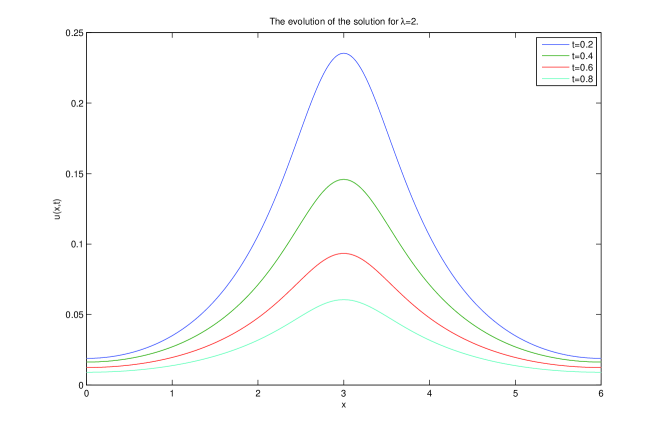
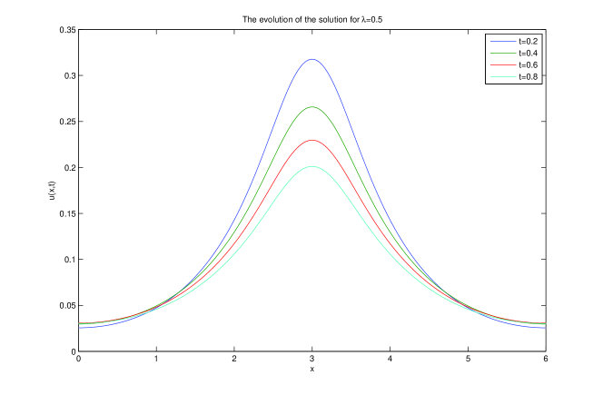
Figure 1: The evolution of the solution for $\alpha=0.3$. $\tau=0.001,h=0.01,k=2.$

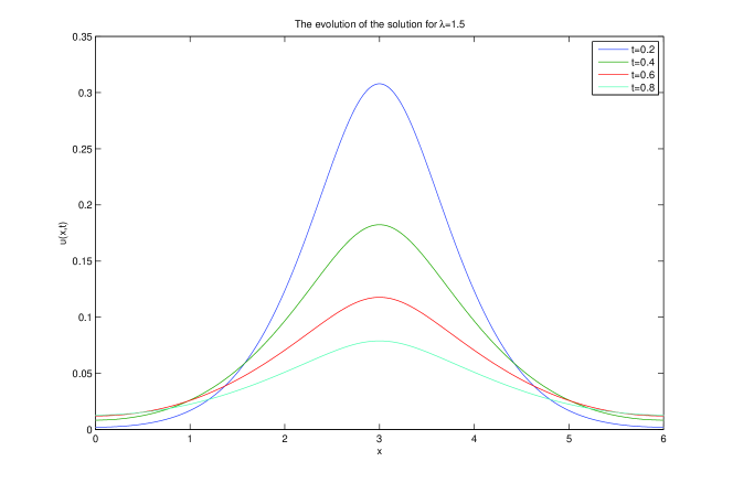
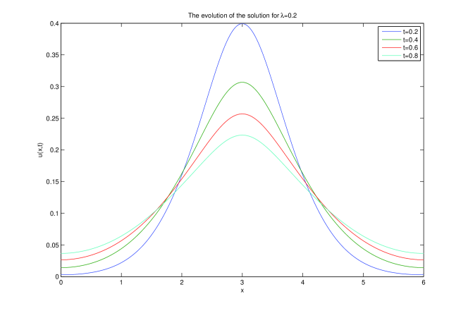
Figure 2: The evolution of the solution for $\alpha=0.8$. $\tau=0.001,h=0.01,k=2.$

6 Conclusion

In this paper we have proposed and analyzed an implicit fully discrete LDG method with the convergent orders $O(h^{k+1}+(\tau)^{2-\alpha})$ for the tempered fractional diffusion equation. Numerical examples are provided to confirm the order of convergence and show the effectiveness of the proposed scheme (2.7). It is worth to mention that the scheme can be extended to solve the two or higher dimensional case easily, and the theoretical results are also valid. However, the computation work will be huge. In future we would like to study this problem and try to design a effective scheme for the two dimensional case.

References

- [1] B. Baeumer and M. M. Meerschaert, Tempered stable Levy motion and transient superdiffusion, J. Comput. Appl. Math., 233 (2010) 2438-2448.
- [2] R. N. Mantegna and H. E. Stanley, Stochastic process with ultraslow convergence to a Gaussian: The truncated Levy flight, Phys. Rev. Lett., 73 (1994) 2946-2949.
- [3] M. M. Meerschaert, Y. Zhang, and B. Baeumer, Tempered anomalous diffusion in heterogeneous systems, Geophys. Res. Lett., 35 (2008) 190201.
- [4] A. Cartea, D. del-Castillo-Negrete, Fractional diffusion models of option prices in markets with jumps, Phys. A, 374(2007) 749-763.
- [5] S. Chen, J. Shen, L.L. Wang, Generalized Jacobi functions and their applications to fractional differential equations, Math. Comp., 85 (2016) 1603-1638.
- [6] M. R. Cui, Compact finite difference method for the fractional diffusion equation, J. Comput. Phys., 228 (2009) 7792-7804.
- [7] Y. Cheng, X. Meng, Q. Zhang, Application of generalized Gauss-Radau projections for the local discontinuous Galerkin method for linear convection-diffusion equations, Math. Comp., 86 (2017) 1233-1267
- [8] V.J. Ervin, J.P. Roop, Variational formulation for the stationary fractional advection dispersion equation, Numer. Methods Partial Differential Eq., 22(2005) 558-576.
- [9] J.L. Gracia, M. Stynes, Central difference approximation of convection in Caputo fractional derivative two-point boundary value problems, J. Comput. Appl. Math., 273 (2015) 103-115.
- [10] E. Hanert, C. Piret, A Chebyshev pseudospectral method to solve the space-time tempered fractional diffusion equation, SIAM J. Sci. Comput., 36 (2014) 1797-1812.
- [11] Z. Hao, W. Cao, G. Lin, A second-order difference scheme for the time fractional substantial diffusion equation, J. Comput. Appl. Math., 313 (2017) 54-69.
- [12] Y.Jiang, J. Ma, High-order finite element methods for time-fractional partial differential equations, J. Comput. Appl. Math., 235(2011) 3285-3290.
- [13] B. Jin, R. Lazarov, Z. Zhou, An analysis of the L1 scheme for the subdiffusion equation with nonsmooth data, IMA J. Numer. Anal., 36 (2016) 197-221.
- [14] I. Koponen, Analytic approach to the problem of convergence of truncated L¡äevy flights towards the Gaussian stochastic process, Phys. Rev. E, 52 (1995) 1197-1199.
- [15] L. Feng, P. Zhuang, F. Liu, I. Turner, Y. Gu, Finite element method for space-time fractional diffusion equation, Numer. Algor., 72 (2016) 749-767
- [16] T. A. M. Langlands and B. I. Henry, The accuracy and stability of an implicit solution method for the fractional diffusion equation, J. Comput. Phys., 205 (2005) 719-736.
- [17] M. Li, X. Gu, C. Huang, etc, A fast linearized conservative finite element method for the strongly coupled nonlinear fractional Schrdinger equations, J. Compu. Phys., 358(2018) 256-282.
- [18] C.P. Li, F.H. Zeng, Numerical methods for fractional calculus, CRC Press, Boca Raton, FL, 2015.
- [19] C. Li, W. Deng, High order schemes for the tempered fractional diffusion equations, Adv. Comput. Math., 42 (2014) 543-572.
- [20] X. Li and C. Xu, A space-time spectral method for the time fractional diffusion equation, SIAM J. Numer. Anal., 47 (2009) 2108-2131.
- [21] S.J. Liao, Notes on the homotopy analysis method: some definitions and theorems, Commun Nonlinear Sci Numer Simul., 14 (2009) 983-997.
- [22] Y.M. Lin, C.J. Xu, Finite difference/spectral approximations for the time-fractional diffusion equation, J. Comput. Phys., 225 (2007) 1533-1552.
- [23] F.W. Liu, P.H. Zhuang, Q.X. Liu, The Applications and Numerical Methods of Fractional Differential Equations, Science Press, Beijing, 2015.
- [24] S. Momani and Z. Odibat, Comparison between the homotopy perturbation method and the variational iteration method for linear fractional partial differential equations, Comput. Math. Appl., 54 (2007) 910-919.
- [25] J.Q. Murillo, S.B. Yuste, On three explicit difference schemes for fractional diffusion and diffusion-wave equations, Phys. Scr., 136 (2009) 14025-14030.
- [26] M.M. Meerschaert, C. Tadjeran, Finite difference approximations for fractional advection-dispersion ow equations, J. Comput. Appl. Math., 172 (2004) 65-77.
- [27] X. Meng, C.-W. Shu, and B. Wu, Optimal error estimates for discontinuous Galerkin methods based on upwind-biased fluxes for linear hyperbolic equations, Math. Comp., 85 (2016), no. 299, 1225-1261, DOI 10.1090/mcom/3022. MR3454363
- [28] J. Rosinski, Tempering stable processes, Stochastic Process. Appl., 117 (2007) 677-707.
- [29] E. Sousa, C. Li, A weighted finite difference method for the fractional diffusion equation based on the Riemann-Liouville derivative, Appl. Numer. Math., 90 (2015) 22-37.
- [30] Z.Z. Sun, X.N. Wu, A fully discrete difference scheme for a diffusion-wave system, Appl. Numer. Math., 56 (2006) 193-209.
- [31] H. Wang, D. Yang, S. Zhu, Inhomogeneous Dirichlet boundary-value problems of space-fractional diffusion equations and their finite element approximations. SIAM J. Numer. Anal., 52 (2014) 1292-1310.
- [32] L. Wei, X. Zhang, Y. He, Analysis of a local discontinuous Galerkin method for time-fractional advection-diffusion equations, Int. J. Heat. Fluid. Fl., 23(2013) 634-648.
- [33] L. Wei, Y. He, Analysis of a fully discrete local discontinuous Galerkin method for time-fractional fourth-order problems. Appl. Math. Model., 38 (2014) 1511-1522.
- [34] Y. Xia, Y. Xu and C.-W. Shu, Application of the local discontinuous Galerkin method for the Allen-Cahn/Cahn-Hilliard system, Commun. Comput. Phys., 5 (2009) 821-835.
- [35] Y. Xu, C.-W. Shu, Local discontinuous Galerkin methods for high-order time-dependent partial differential equations, Comm. Comput. Phys., 7 (2010) 1-46.
- [36] Y.Y. Yu, W. H. Deng, Y.J. Wu, Third order difference schemes (without using points outside of the domain) for one sided space tempered fractional partial differential equations, Appl. Numer. Math., 112 (2017) 126-145.
- [37] H. Zhang, F. Liu, I. Turner, S. Chen, The numerical simulation of the tempered fractional Black-Scholes equation for European double barrier option, Appl. Math. Model., 40(2016) 5819-5834.
- [38] Y.M. Zhao, Y.Zhang, F. Liu, I. Turner, Y. Tang, V.Anh, Convergence and superconvergence of a fully-discrete scheme for multi-term time fractional diffusion equations, Comput. Math. Appl., 73(2017) 1087-1099.
- [39] Q. Zhang and F.-Z. Gao, Explicit Runge-Kutta local discontinuous Galerkin method for convection dominated Sobolev equation, J. Sci. Comput., 51 (2012) 107-134.
- [40] Q. Zhang, C.-W. Shu, Error estimate for the third order explicit Runge-Kutta discontinuous Galerkin method for a linear hyperbolic equation with discontinuous initial solution, Numer. Math. 126 (2014) 703-740.