Single-Bit Consensus with Finite-Time Convergence: Theory and Applications

Abstract

In this brief paper, a new consensus protocol based on the sign of innovations is proposed. Based on this protocol each agent only requires single-bit of information about its relative state to its neighboring agents. This is significant in real-time applications, since it requires less computation and/or communication load on agents. Using Lyapunov stability theorem the convergence is proved for networks having a spanning tree. Further, the convergence is shown to be in finite-time, which is significant as compared to most asymptotic protocols in the literature. Time-variant network topologies are also considered in this paper, and final consensus value is derived for undirected networks. Applications of the proposed consensus protocol in (i) 2D/3D rendezvous task, (ii) distributed estimation, (iii) distributed optimization, and (iv) formation control are considered and significance of applying this protocol is discussed. Numerical simulations are provided to compare the protocol with the existing protocols in the literature.

Index Terms – Consensus, Finite-time convergence, Lyapunov stability theorem, Graph theory, Rendezvous, Formation control

I Introduction

Consensus protocols [1, 2, 3, 4, 5, 6] have recently found applications in many disciplines including control [7] and signal processing [8, 9, 10, 11] literature. For consensus, a group of sensors/estimators/agents reach an agreement on state values, where state may represent different quantities and parameters of interest; for example, the state may be the velocity of Unmanned Aerial Vehicles (UAVs) while moving as a flock [1] or it may represent the temperature/wind-speed in geographical fields to be estimated [9]. In this scenario, a sensor network reaches consensus on measurements and/or state innovations to estimate the underlying system state. Also, in distributed detection agents share information to reach consensus on Log-Likelihood Ratio (LLR) [12] or scalar-valued decision statistic [13]. One possible application is in distributed estimation [9, 10, 11, 14, 15] with further application in spacecraft attitude estimation [16, 17]. Further, in control literature, consensus finds applications in distributed optimization [18], flight formation [19, 20, 21, 22], and multi-agent rendezvous [23, 24]. Of particular interest in aerospace system applications, along with rendezvous in 3D space, are distributed target tracking [25] and formation control via a group of UAVs. For example, in distance-based formation control the consensus protocol is used to stabilize the UAVs to form a specific geometric shape (see Section V-D for more information).

This paper proposes a single-bit consensus with ability to converge in finite-time. The main feature of this consensus protocol is the single-bit information update. The consensus protocol is proposed based on the sign of difference between state values. This implies that only single-bit of information (the sign) is required to update the state of the agents. This reduces the amount of processing/computation load and/or network communication load at each agent. It should be emphasized that in applications with real-time data processing where the computation and communication are required in faster time scale, the less computation and/or communication load is a significant merit. Since the protocol is nonlinear, a new Lyapunov function is proposed to prove consensus stability. Further, it is proved that for the proposed single-bit consensus protocol the Lyapunov function vanishes in finite-time, implying the finite-time convergence of the consensus protocol. In [4, 5, 6] finite-time consensus protocols are proposed, however these protocols impose large amount of computation on agents and are computationally less efficient than the proposed single-bit protocol in this paper.

Quantized consensus [12, 26, 27] is a related concept, where the agents reach consensus on quantized information with finite quantization levels for possibly unbounded data. In this direction [27] investigates a deterministic quantization based on alternating direction method of multipliers (ADMM). In [12] authors adopt a single-bit quantized consensus method for detection based on Bayesian criterion and Neyman-Pearson criterion. In [13] the authors propose two consensus+innovation type distributed detectors based on Generalized Likelihood-Ratio Test (GLRT) for composite hypothesis testing via a group of sensors. Further, communication in multi-agent systems based on single-bit of information is also adopted in distributed detection [28, 29]. In these works a group of sensors are spatially distributed over a surveillance field to locally detect the existence of an uncooperative target and then communicate their single-bit decisions to a fusion center. The single-bit decisions are based on either the hybrid combination of GLRT and Bayesian estimation [29] or Generalized-Rao Test [28]. The fusion center combines the received information based on the fusion rules and makes a global decision.

The main contributions of this paper are as follows: (i) the proposed protocol is based on single-bit of information, which makes it practical in real-time system applications. This is the most important feature of our proposed protocol. (ii) a new Lyapunov function is proposed to prove the stability and convergence of this nonlinear consensus protocol under certain connectivity condition. This Lyapunov function is irrespective of the consensus protocol dynamics, and therefore, might be used for stability analysis of other nonlinear consensus protocols in the literature [2, 4]. (iii) the convergence time of the consensus is in finite-time while reducing the computation load on agents in contrast to most asymptotic consensus protocols in the literature [1, 2]. It should be noted, although finite-time consensus protocols are already exist in the literature, to name a few [4, 5, 6], their main drawback is their computational complexity as compared to the proposed protocol in this paper.

The rest of the paper is organized as follows: Section II formulates the new consensus protocol. Section III provides the proof of consensus and convergence based on Lyapunov stability. Section IV provides the convergence condition in case of time-variant switching network topologies. Section V provides some applications of the proposed protocol. Section VI presents simulation to verify the results, and finally Section VII concludes the paper.

II New Consensus Protocol

Assume a network of $n$ agents with ability to process information and communicate with neighboring agents to share information. The communication network of agents is represented by graph $\mathcal{G}=(\mathcal{V},\mathcal{E},W)$, where $\mathcal{V}=\{1,...,n\}$ represents the set of graph nodes (agents), $\mathcal{E}$ represents the set of edges (communication links) defined as $\mathcal{E}=\{(i,j)|W_{ji}\neq 0\}$. Note that $W_{ji}\neq 0$ is the weight assigned to communication link from node $i$ to node $j$. Further, the neighborhood of agent $i$ is defined as $\mathcal{N}_{i}=\{j\in\mathcal{V}|W_{ij}\neq 0\}$

The state of each agent is represented by $x_{i}$ and $\mathbf{x}=[x_{1},...,x_{n}]^{\top}$ represents the state of all agents. The following consensus protocol is proposed to update the state of agent $i$ as:

$$\dot{x}_{i}=\sum_{j=1}^{n}W_{ij}\text{sgn}(x_{j}-x_{i})=\sum_{j\in\mathcal{N}_{i}}W_{ij}\text{sgn}(x_{j}-x_{i})$$ (1)

where $\text{sgn}()$ is the sign function defined as:

$$\text{sgn}(x)=\begin{cases}1&\quad\text{if }x>0\\ -1&\quad\text{if }x<0\\ \end{cases}$$ (2)

where the $|x_{j}-x_{i}|$ represents the absolute value of $(x_{j}-x_{i})$. Notice that consensus protocol (1) only requires the sign of $(x_{j}-x_{i})$, which can be defined by single-bit of information.

Extending the scalar-state protocol (1) to vector-state $\mathbf{x}$, the updating law is as follows:

$$\dot{\mathbf{x}}_{i}=\sum_{j\in\mathcal{N}_{i}}W_{ij}\frac{\mathbf{x}_{j}-\mathbf{x}_{i}}{\|\mathbf{x}_{j}-\mathbf{x}_{i}\|}$$ (3)

where $\|.\|$ represents the Euclidean norm of the vector. In this case, the agents use the weighted summation of the unit vector of its state relative to its neighbors’ states for control update.

In both cases of scalar-valued consensus (1) and vector-state consensus (3) the amount of information exchange and/or the computation on agents is less than the common consensus protocols in the literature [1, 2, 4, 5, 6]. In protocol (1) only the sign of relative states $x_{j}-x_{i}$ is needed to be exchanged among agents and to be computed for state update. Similarly, for protocol (3) only unit vector in the direction of relative state vector is needed for computation and communication. This is the key feature reducing the amount of information exchange and/or computational load at each agent and improving the real-time feasibility of the protocol.

Now the question is how the agents exchange information on the sign function or unit vector. This depends on the nature of agents’ states. Assume the state represents the position or velocity of the agent. For consensus on scalar-valued velocities, for example in flocks or vehicle platooning [30], following protocol (1) each agent only needs to know if the other agent moves faster or slower, without needing to exactly know the velocity of the neighboring agent by communication or sensing the exact velocity. For consensus on position vectors as in (3) each agent uses the unit vector in the direction of relative positions of neighboring agents and, in contrast to protocols in the literature, there is no need to communicate exact positions of agents. This can be done, for example, by omni-directional cameras on agents without need to communicate exact locations (See more explanations on this in Section V-A). Then, the agents update their state (position) based on the weighted summation of these unit vectors. In scalar-state case, the state of agent $i$ is updated based on the weighted summation of $1$s and $-1$s, where $1$ and $-1$ are respectively assigned to the case $x_{j}>x_{i}$ and $x_{j}<x_{i}$. The agents’ states get updated and evolve in time until all the agents have the same state and reach consensus. It should be mentioned that this protocol does not fail for static states. In other words, when the weighted sum of $1$s and $-1$s or the unit vectors is zero, the state of agent does not change. The state remains unchanged until the summation changes due to change in the state of neighboring agents, or the system reaches consensus and the state of all agents remains unchanged and equal.

One drawback of the given protocol (1), and in general any non-Lipschitz protocol, is the sensitivity to time-delay. In case there is time-delay in the information exchange among agents, undesirable oscillations in agents’ states may occur which is known as chattering phenomenon. This is a side-effect of using non-Lipschitz function and is prevalent in finite-time convergent consensus protocols as in [4, 5, 6] and also in Sliding Mode Control (SMC) [31]. One solution to avoid such phenomenon is to use smooth Lipschitz functions around the equilibrium, for example saturation function,

$$\text{sat}(x)=\begin{cases}1&\quad\text{if }x>a\\ x&\quad\text{if}-a<x<a\\ -1&\quad\text{if }x<-a\end{cases}$$ (4)

This is proposed in SMC as described in [31]. In such case the agents’ states reach a convergence ball (of radius $a$) around the equilibrium in finite-time, however, the convergence inside this convergence ball is asymptotic. In terms of information exchange, the agents share single-bit of information outside this convergence ball, while inside this ball they need to share full-state information. For example, when the state represents location, in case agents’ states get closer to each-other the agents are able to share more information, while in distant states only single-bit of information is exchanged. It should be mentioned, replacing the non-Lipschitz function with a Lipschitz equivalent only alleviates the effect of time-delay and does not completely vanish the chattering phenomenon.

III Proof of Finite-Time Convergence

Here, we answer the following question: what is the connectivity requirement on the network such that state of all agents reach the same value? i.e., $\mathbf{x}^{*}=\alpha\mathbf{1}$ is the stable equilibrium point of the protocol (1) under what connectivity condition. To answer this, we introduce the concept of spanning tree in directed graphs. Define a directed tree as a directed graph where every node (except the root node) has exactly one incoming edge. The root node (also referred as leader node) has no incoming edge. A graph has a spanning tree if it contains a directed tree as a subgraph that spans all nodes.

Theorem 1.

Protocol (1) reaches consensus if and only if the communication network $\mathcal{G}$ has a spanning tree.

Proof.

Contradiction is used for the proof. Sufficiency: if the graph $\mathcal{G}$ has a spanning tree, we prove that the equilibrium point of (1) is in the form $\mathbf{x}^{*}=\alpha\mathbf{1}$. As a contradiction assume that $\mathbf{x}^{*}\neq\alpha\mathbf{1}$. Therefore, consider the agent $i$ with maximum (or minimum) state. Since the network has a spanning tree there is at least one agent $j$ in the neighborhood of $i$ (or agent $i$ is in the neighborhood of agent $j$) [32]. Therefore,$\dot{x}_{i}=\sum_{j\in\mathcal{N}_{i}}W_{ij}\text{sgn}(x_{j}-x_{i})<0$ or $\dot{x}_{i}=\sum_{i\in\mathcal{N}_{j}}W_{ji}\text{sgn}(x_{i}-x_{j})>0$ which both cases contradict the definition of equilibrium point. Necessity: If no spanning tree is contained in the communication graph $\mathcal{G}$, it implies that there is no information flow (directed path) at least among two agents. In graph theory, this implies that either the graph has at least two roots or the graph contains at least two unconnected components [32]. In first case, note that $\dot{x}_{root}=0$ since it has no incoming information ($\mathcal{N}_{root}=\emptyset$ [32]). Therefore, the states of two root agents remain the same initial values without updating, and these two agents never reach consensus. In the second case, since there is no information flow (directed path) between two components, each component reaches a consensus value which in general differs from the consensus value of the other component. Therefore, for both cases the consensus may not be reached. ∎

Theorem 2.

In protocol (1), having a spanning tree in $\mathcal{G}$, states of all agents converge to stable consensus equilibrium point $\mathbf{x}^{*}=\alpha\mathbf{1}$ in finite-time.

Proof.

We prove the theorem using Lyapunov stability theorem. Define the following Lyapunov function:

$$V=x_{\max}-x_{\min}$$ (5)

where $x_{\max}$ and $x_{\min}$ are respectively the maximum state value and the minimum state value of the agents, i.e. $x_{\max}=\max\{x_{i},i\in\{1,\dots,n\}\}$ and $x_{\min}=\min\{x_{i},i\in\{1,\dots,n\}\}$ In fact, $x_{\max}$ and $x_{\min}$ are time-dependent, i.e., the agent possessing the max/min value differs at every time instant. Notice that $x_{\max}=x_{\min}$ implies that the max value and min value of all agents are equal and therefore the consensus equilibrium point $\mathbf{x}^{*}=\alpha\mathbf{1}$ is reached. Note that the Lyapunov function $V$ is continuous, regular, and Lipschitz. Also, $V$ is globally positive definite, i.e. $V>0\Leftrightarrow\mathbf{x}^{*}\neq\alpha\mathbf{1}$ and $V=0\Leftrightarrow\mathbf{x}^{*}=\alpha\mathbf{1}$. Further, Lyapunov function $V$ is radially unbounded, i.e. $V\rightarrow\infty$ as $|x_{i}|\rightarrow\infty$. For convergence and stability we prove that $\dot{V}$ is negative definite.

$$\dot{V}=\dot{x}_{\max}-\dot{x}_{\min}$$ (6)

$$\dot{x}_{\max}=\sum_{j\in\mathcal{N}_{\max}}W_{\max j}\text{sgn}(x_{j}-x_{\max})$$ (7)

$$\dot{x}_{\min}=\sum_{j\in\mathcal{N}_{\min}}W_{\min j}\text{sgn}(x_{j}-x_{\min})$$ (8)

Define $\min\{W\}$ as the minimum positive consensus weight of agents in weight matrix $W$. Since the weight matrix $W$ might be time-variant, the term $\min\{W\}$ might be assigned to different agents over time. We have,

$$\dot{x}_{\max}=-\sum_{j\in\mathcal{N}_{\max}}W_{\max j}\leq-\min\{W\}$$ (9)

$$\dot{x}_{\min}=\sum_{j\in\mathcal{N}_{\min}}W_{\min j}\geq\min\{W\}$$ (10)

Therefore, $\dot{V}\leq-2\min\{W\}$ This implies that $\dot{V}$ is globally negative definite, i.e. $\dot{V}<0\Leftrightarrow\mathbf{x}^{*}\neq\alpha\mathbf{1}$ and $\dot{V}=0\Leftrightarrow\mathbf{x}^{*}=\alpha\mathbf{1}$. Therefore, based on Lyapunov stability theorem [31] the consensus point is globally stable equilibrium of protocol (1).

Further let $t_{cons}$ be the convergence time of the consensus protocol (1).

$$\int_{0}^{t_{cons}}\dot{V}\leq-\int_{0}^{t_{cons}}2\min\{W\}$$ (11)

$$V(t_{cons})-V(0)\leq-2\min\{W\}t_{cons}$$ (12)

$${t_{cons}}\leq\frac{x_{\max}(0)-x_{\min}(0)}{2\min\{W\}}$$ (13)

representing finite-time upperbound on conevergence. ∎

One point to be noted in the proof of Theorem 2 is on the notation of $x_{max}$, $x_{min}$, $\mathcal{N}_{\max}$, $\mathcal{N}_{\min}$, and $W_{\max j}$. For these terms max/min values do not necessarily concern a single agent over time, but these max/min values concern all agents. In other words, the agent possessing the min/max value, its neighbors, and the associated weights change over time, and therefore, the time-evolution of the Lyapunov function (5) is not necessarily smooth.

It should be noted, the proof of the stability and convergence for the vector-state protocol (3) follows similar Lyapunov analysis. In vector-state problem, the Lyapunov function can be considered as the perimeter of the convex hull containing the vector state of the agents, or the circumference of the smallest covering ball/circle enclosing the vector states. Following similar analysis as in above, it can be proved that the Lyapunov function is always decreasing under protocol (3).

IV Time-Variant Network Topologies

Note that the consensus network of agents may change in time due to failure or addition of new links among agents. This may particularly happen in network of mobile agents where the communication range of agents are limited or in real world applications due to obstacles. The objective of this section is to determine the conditions on changing network topology $\mathcal{G}$ for which the consensus can be reached. The main point in this section is that our proposed Lyapunov function does not depend on the graph topology $\mathcal{G}$.

Theorem 3.

Consider the network topology of agents to be selected from the finite set of graphs $\Gamma_{m}=\{\mathcal{G}_{1},\mathcal{G}_{2},...,\mathcal{G}_{m}\}$, where $\mathcal{G}_{d}=(\mathcal{V},\mathcal{E}_{d},W_{d}),d\in\{1,...,m\}$. Agents reach consensus under protocol (1) if for a sufficient sequence of bounded non-overlapping time-intervals $[t_{k},t_{k}+l_{k}],~{}k=1,2,...$, the combination of network topologies across each time-interval contain a spanning-tree.

Proof.

Again consider the proposed positive definite Lyapunov function $V=x_{\max}-x_{\min}$ which is independent of network topology. The proof is similar to the proof of Theorem 2. Note that in every time-interval $[t_{k},t_{k}+l_{k}]$ the combination of graph topologies contain a spanning tree. Therefore, the agent with $x_{\max}$ (or $x_{\min}$) has at least one neighbor $j$ or is a neighbor of agent $j$ in a sub-domain of the interval (not necessarily in the entire time-interval). This implies that for this time domain $\dot{x}_{\max}\leq-min\{W\}$ (or $\dot{x}_{\min}\geq min\{W\}$). Consequently, following the statement of the proof in Theorem 2, in this time domain $\dot{V}$ is negative definite and more precisely $\dot{V}\leq-2\min\{W\}$. This implies that after sufficient (finite) number of time-intervals the Lyapunov function reaches $0$ and consensus is achieved. ∎

V Applications

V-A Rendezvous in 2D/3D space

In rendezvous problem [23, 24], the goal is to devise control strategies on a group of mobile agents to eventually move them to a single location The state of each agent is its position in 2D/3D space, and the aim is to reach a consensus on the position. In words, each agent applies the weighted summation of the unit vector relative to its neighbors’ positions to update its own location. In fact, using protocol (3), every agent only needs to be informed of the direction of the neighboring agent’s relative position vector, but not its magnitude. This is significant as by using, for example, omni-directional cameras [33] each agent finds information on the relative direction towards its neighbor’s position, and there is no need to communicate the exact location of the agents. This approach can be implemented, for example, to improve the experimental results in [34] in terms of real-time communication and computation; each robot only needs to find the direction that the neighboring robots are located using an omni-directional camera and there is no need to communicate its position to the neighboring robots. This, further, can be extended to the 3D case to implement the rendezvous task over a network of UAVs.

V-B Distributed estimation

In single time-scale distributed estimation [9, 10, 11, 14] the idea is to track the state of the dynamical system via a network of agents. Consider a noisy system monitored by noise-corrupted measurements,

$$\mathbf{x}^{k+1}=A\mathbf{x}^{k}+\mathbf{v}^{k},$$ (14)

$$\mathbf{y}^{k}_{i}=H_{i}\mathbf{x}^{k}+\mathbf{r}^{k}_{i}.$$ (15)

In the above formulation, $A$ is the dynamical system matrix, $k$ is the time-step, $y^{k}_{i}$ is the measurement of agent $i$ at time-step $k$, and ${v}^{k}$ and ${r}^{k}_{i}$ are the noise terms. Following the distributed estimation protocol in [10, 35, 36, 37, 38], the following protocol based on the consensus-update law (3) is considered:

$$\tilde{\mathbf{x}}_{i}^{k} = \sum_{j\in\mathcal{N}_{\beta}(i)}W_{ij}A\widehat{\mathbf{x}}_{j}^{k-1}$$

$$\widehat{\mathbf{x}}_{i}^{k} = \tilde{\mathbf{x}}_{i}^{k}+K_{i}^{k}\sum_{j\in\mathcal{N}_{\alpha}(i)}H_{j}^{\top}\left(\frac{\mathbf{y}^{k}_{j}-H_{j}\tilde{\mathbf{x}}_{i}^{k}}{\|\mathbf{y}^{k}_{j}-H_{j}\tilde{\mathbf{x}}_{i}^{k}\|}\right).$$ (16)

where, $\mathcal{N}_{\alpha}(i)$ and $\mathcal{N}_{\beta}(i)$ represent some specific neighborhoods of agent $i$, and $K^{k}_{i}$ is the estimation gain at agent $i$ (see the previous works by author [10, 35, 36, 37, 38] for more information). One interesting extension to distributed estimation protocol (16) may be considered for the case of sensor failure and countermeasures to recover for that (see more information in [37].)

One application of the above distributed estimation scenario is in target tracking based on time-difference-of-arrival (TDOA) via a group of UAVs [25]. In this framework a group of UAVs estimate the location of a mobile target based on the time-difference-of-arrival of some beacon signal received by the UAVs. Each UAV shares the TDOA-based information with its neighboring UAVs, and also shares the estimated position of the target. Then, by consensus averaging of the position estimates and information fusion on the state-predictions, each UAV in the network can localize the source, and the group tracks the location of the mobile target.

V-C Distributed optimization

In distributed optimization problem [18] the objective is to distributively solve the following optimization problem via a multi-agent network,

$$\min\limits_{x\in\mathbb{R}}~{}~{}f(x):=\frac{1}{n}\sum_{i=1}^{N}f_{i}(x)$$ (17)

where $f(x)$ is the continuously convex objective function and $f_{i}(x)$ is the local objective function only known by agent $i$. The distributed gradient-descent-based solution for this problem applying the consensus protocol (1) is as follows,

$$x^{k+1}_{i}=x^{k}_{i}-\alpha^{k}\nabla f_{i}(x_{i}^{k})+\gamma\alpha^{k}\sum_{j\in\mathcal{N}_{i}}W_{ij}\text{sgn}(x^{k}_{j}-x^{k}_{i})$$ (18)

where $\gamma>0$ is a scalar weight and $\alpha^{k}$ is the optimization step-size at time $k$.

The protocol (18) reduces the amount of information processing and computation load on agents as compared to [18], particularly in large scale applications. Note that each agent only relies on the sign of relative state of neighboring agents. In the same line of research, [26] considers the case that the communicated decision information among agents are quantized in order to alleviate the communication bottleneck in distributed optimization. The authors propose a Quantized Decentralized Gradient Descent (QDGD) and prove the convergence of their protocol for strongly convex and smooth local cost functions.

V-D Formation control of UAVs

One application within the aerospace systems is cooperative control of UAV formation [19, 20, 21, 22]. A group of autonomous UAVs form a pre-specified formation setup (e.g. a star-shaped formation) in which two neighboring UAVs $i$ and $j$ are in the distance $d_{ij}$ based on their formation shape. The control input to the group of UAVs are designed such that they can move along on this formation without collision in order to, for example, track a mobile target or avoid an obstacle. One example of such formation control scenario is given as following. Define $\mathbf{x}_{i}$ as the position of UAV (or agent) $i$ in 3D space evolving in time as:

$$\dot{\mathbf{x}}_{i} = \mathbf{p}_{i}$$

$$\dot{\mathbf{p}}_{i} = \sum_{j\in\mathcal{N}_{i}}W_{ij}\left(\frac{\mathbf{x}_{j}-\mathbf{x}_{i}}{\|\mathbf{x}_{j}-\mathbf{x}_{i}\|}\right)-\bar{u}\lambda_{2}\sigma(\mathbf{p}_{i}).$$ (19)

where $\bar{u}>0$, $\sigma(\mathbf{y})=\mathbf{y}/\sqrt{(1+\|\mathbf{y}\|^{2})}$, and

$$W_{ij}:=\frac{\bar{u}\lambda_{1}}{|\mathcal{N}_{i}|}\sigma(\|\mathbf{x}_{i}-\mathbf{x}_{j}\|-d_{ij})$$ (20)

with $0<\lambda_{1},\lambda_{2}<1$, $\lambda_{1}+\lambda_{2}=1$. Note that the above formation protocol is a distance-based approach, where the final formation of agents depend on the rigidity of the neighboring graph, and is also based on the distance $d_{ij}$ of every two agents $i$ and $j$ in forming the geometric shape.

VI Simulation

For simulation we consider network of $10$ agents with random initial states in $[0,10]$. Assume the network is time-variant and switches every $0.4$ seconds between the graph topologies shown in Fig.1.

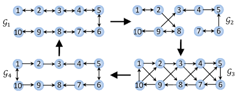
Figure 1: This figure shows the change in network topology of agents. The graphs $\mathcal{G}_{1}$ and $\mathcal{G}_{3}$ contain a spanning tree, while graphs $\mathcal{G}_{2}$ and $\mathcal{G}_{4}$ contain no spanning tree.

As it can be seen from the figure, graph $\mathcal{G}_{1}$ is connected undirected and contains a spanning tree. Graph $\mathcal{G}_{2}$ is connected with no spanning tree. $\mathcal{G}_{3}$ represents a strongly connected graph having a spanning tree. Finally, $\mathcal{G}_{4}$ contains no spanning tree as a subgraph. To check the conditions of Theorem 3 for consensus convergence, note that the combination of the network in time domain of every $0.8$ seconds contain a spanning tree. This implies that consensus can be reached, as it is shown in Fig.2. This figure shows that the difference of state values ($x_{\max}-x_{\min}$) is decreasing over time and all agents reach a consensus value.

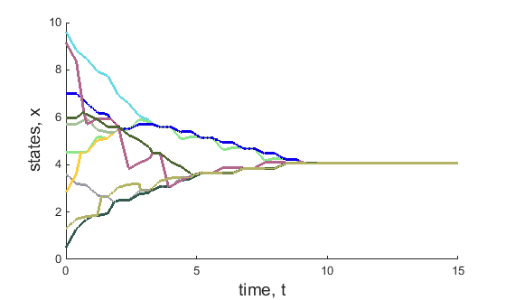
Figure 2: This figure shows the state-evolutions in time under the single-bit protocol (1) while agents’ connectivity follows the switching topologies given in Fig.1. As it can be seen $x_{max}-x_{min}$ is decreasing in time and the consensus among agents is achieved in finite-time.

To compare our results, the time-evolution of the Lyapunov function (5) for our proposed consensus protocol along with six other consensus protocols from [1, 2, 4, 5, 6] are shown in Fig.3. In this simulation $\alpha=0.25$ for protocol in [4], $\alpha=0.5$ for protocol in [5], $\alpha=0.8$, $\beta=1.2$, $p=3$, and $q=5$ for protocol in [6], $\alpha=0.4$ for protocols in [2]. All these protocols are evaluated over switching network topologies (Fig. 1) with the same initial state values of agents. As it can be seen, the linear average consensus [1], the geometric consensus [2], and the harmonic consensus [2] all reach asymptotic stability while the convergence of the other four protocols are in finite-time. The Lyapunov function for our proposed protocol (and the six other protocols) is decreasing over time ($\dot{V}\leq 0$) which implies Lyapunov stability.

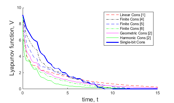
Figure 3: This figure shows the time evolution of Lyapunov function (5) for seven consensus protocols: the blue solid line represents the proposed protocol (Lyapunov function of states in Fig.2) and other lines are for protocols in [1, 2, 4, 5, 6]. The Lyapunov function is decreasing for all consensus protocols and reaches zero in finite-time for protocols [4, 5, 6] along with single-bit protocol and reaches zero asymptotically for protocols in [1, 2].

VII Conclusions

Note that the protocol is based on computation and communication of single-bit of information and unit vector on state update. This makes the protocol more feasible in terms of real-time applications, since it requires less computational load and information exchange among agents. The known protocols in the literature require the calculation of the exact relative state $x_{j}-x_{i}$ or a function of it $f(x_{j}-x_{i})$, however this protocol only requires the single-bit information on sign of $x_{j}-x_{i}$. In other words, the agent $i$ only needs to know for neighboring agent $j$ if $x_{j}<x_{i}$ or $x_{j}>x_{i}$. Similarly, for vector state consensus the agent $i$ only need to know the unit-vector in the direction of relative state vector, e.g. by use of omni-directional cameras in rendezvous problem as discussed in Section V-A. This is more real-time feasible in terms of computational complexity and communication load on agents.

The consensus protocol in this paper may be used to decentralize the information fusion in [28, 29]. In this case the information on detecting the existence or absence of the target may be shared by agents in their neighborhood via an undirected communication network and agents eventually average the received information via the proposed protocol and reach a consensus on detecting the target. However, this approach may result in performance degradation as compared to advanced GLRT or G-Rao fusion methods.

References

- [1] R. Olfati-Saber, J. A. Fax, and R. M. Murray, “Consensus and cooperation in networked multi-agent systems,” Proceedings of the IEEE, vol. 95, no. 1, pp. 215–233, Jan. 2007.
- [2] D. Bauso, L. Giarré, and R. Pesenti, “Nonlinear protocols for optimal distributed consensus in networks of dynamic agents,” Systems & Control Letters, vol. 55, no. 11, pp. 918–928, 2006.
- [3] H. Sayyaadi and M. Doostmohammadian, “Finite-time consensus in directed switching network topologies and time-delayed communications,” Scientia Iranica, vol. 18, no. 1, pp. 75–85, 2011.
- [4] L. Wang and F. Xiao, “Finite-time consensus problems for networks of dynamic agents,” IEEE Transactions on Automatic Control, vol. 55, no. 4, pp. 950–955, 2010.
- [5] X. Liu, J. Lam, W. Yu, and G. Chen, “Finite-time consensus of multiagent systems with a switching protocol,” IEEE Transactions on Neural Networks and Learning Systems, vol. 27, no. 4, pp. 853–862, 2015.
- [6] Z. Zuo and L. Tie, “A new class of finite-time nonlinear consensus protocols for multi-agent systems,” International Journal of Control, vol. 87, no. 2, pp. 363–370, 2014.
- [7] S. Park and N. Martins, “Necessary and sufficient conditions for the stabilizability of a class of LTI distributed observers,” in 51st IEEE Conference on Decision and Control, 2012, pp. 7431–7436.
- [8] M. O. Sayin and S. S. Kozat, “Single bit and reduced dimension diffusion strategies over distributed networks,” IEEE Signal Processing Letters, vol. 20, no. 10, pp. 976–979, 2013.
- [9] S. Das and J. M. F. Moura, “Consensus+ innovations distributed kalman filter with optimized gains,” IEEE Transactions on Signal Processing, vol. 65, no. 2, pp. 467–481, 2017.
- [10] M. Doostmohammadian and U. Khan, “On the genericity properties in distributed estimation: Topology design and sensor placement,” IEEE Journal of Selected Topics in Signal Processing, vol. 7, no. 2, pp. 195–204, 2013.
- [11] M. Doostmohammadian and U. A. Khan, “On the distributed estimation of rank-deficient dynamical systems: A generic approach,” in 38th International Conference on Acoustics, Speech, and Signal Processing, Vancouver, CA, May 2013, pp. 4618–4622.
- [12] S. Zhu and B. Chen, “Distributed detection in ad-hoc networks through quantized consensus,” IEEE Transactions on Information Theory, vol. 64, no. 11, pp. 7017–7030, 2018.
- [13] A. K. Sahu and S. Kar, “Recursive distributed detection for composite hypothesis testing: Nonlinear observation models in additive gaussian noise,” IEEE Transactions on Information Theory, vol. 63, no. 8, pp. 4797–4828, 2017.
- [14] M. Doostmohammadian, H. R. Rabiee, and U. A. Khan, “Cyber-social systems: modeling, inference, and optimal design,” IEEE Systems Journal, 2019.
- [15] M. Doostmohammadian and U. A. Khan, “On the characterization of distributed observability from first principles,” in 2nd IEEE Global Conference on Signal and Information Processing, 2014, pp. 914–917.
- [16] J. L. Crassidis and F. L. Markley, “Unscented filtering for spacecraft attitude estimation,” Journal of guidance, control, and dynamics, vol. 26, no. 4, pp. 536–542, 2003.
- [17] S. Roy and R. A. Iltis, “Decentralized linear estimation in correlated measurement noise,” IEEE Transactions on Aerospace and Electronic Systems, vol. 27, no. 6, pp. 939–941, 1991.
- [18] A. Nedić and A. Olshevsky, “Distributed optimization over time-varying directed graphs,” IEEE Transactions on Automatic Control, vol. 60, no. 3, pp. 601–615, 2014.
- [19] S. S. Kia, B. Van Scoy, J. Cortes, R. A Freeman, K. M. Lynch, and S. Martinez, “Tutorial on dynamic average consensus: The problem, its applications, and the algorithms,” IEEE Control Systems Magazine, vol. 39, no. 3, pp. 40–72, 2019.
- [20] R. Olfati-Saber and R. M. Murray, “Distributed cooperative control of multiple vehicle formations using structural potential functions,” IFAC Proceedings Volumes, vol. 35, no. 1, pp. 495–500, 2002.
- [21] R. Padhi, P. R. Rakesh, and R. Venkataraman, “Formation flying with nonlinear partial integrated guidance and control,” IEEE Transactions on Aerospace and Electronic Systems, vol. 50, no. 4, pp. 2847–2859, 2014.
- [22] A. Zou and K. Kumar, “Distributed attitude coordination control for spacecraft formation flying,” IEEE Transactions on Aerospace and Electronic Systems, vol. 48, no. 2, pp. 1329–1346, 2012.
- [23] J. Cortés, S. Martínez, and F. Bullo, “Robust rendezvous for mobile autonomous agents via proximity graphs in arbitrary dimensions,” IEEE Transactions on Automatic Control, vol. 51, no. 8, pp. 1289–1298, 2006.
- [24] W. Ren, R. W. Beard, and E. M. Atkins, “Information consensus in multivehicle cooperative control,” IEEE Control systems magazine, vol. 27, no. 2, pp. 71–82, 2007.
- [25] O. Ennasr, G. Xing, and X. Tan, “Distributed time-difference-of-arrival (tdoa)-based localization of a moving target,” in IEEE 55th Conference on Decision and Control. IEEE, 2016, pp. 2652–2658.
- [26] A. Reisizadeh, A. Mokhtari, H. Hassani, and R. Pedarsani, “Quantized decentralized consensus optimization,” in 2018 IEEE Conference on Decision and Control (CDC). IEEE, 2018, pp. 5838–5843.
- [27] S. Zhu and B. Chen, “Quantized consensus by the admm: Probabilistic versus deterministic quantizers,” IEEE Transactions on Signal Processing, vol. 64, no. 7, pp. 1700–1713, 2015.
- [28] D. Ciuonzo, P. S. Rossi, and P. Willett, “Generalized rao test for decentralized detection of an uncooperative target,” IEEE Signal Processing Letters, vol. 24, no. 5, pp. 678–682, 2017.
- [29] D. Ciuonzo and P. S. Rossi, “Distributed detection of a non-cooperative target via generalized locally-optimum approaches,” Information Fusion, vol. 36, pp. 261–274, 2017.
- [30] M. Pirani, E. Hashemi, A. Khajepour, B. Fidan, B. Litkouhi, S. Chen, and S. Sundaram, “Cooperative vehicle speed fault diagnosis and correction,” IEEE Transactions on Intelligent Transportation Systems, vol. 20, no. 2, pp. 783–789, 2018.
- [31] J.J. Slotine and W. Li, Applied nonlinear control, Prentice-Hall, 1991.
- [32] R. Diestel, Graph theory, Springer Publishing Company, Incorporated, 2017.
- [33] T. Kato, M. Nagata, H. Nakashima, and K. Matsuo, “Localization of mobile robots with omnidirectional camera,” World Academy of Science, Engineering and Technology International Joumal of Computer, Control, Quantum and Information Engineering, vol. 8, no. 7, 2014.
- [34] W. Ren, H. Chao, W. Bourgeous, N. Sorensen, and Y. Chen, “Experimental validation of consensus algorithms for multivehicle cooperative control,” IEEE Transactions on Control Systems Technology, vol. 16, no. 4, pp. 745–752, 2008.
- [35] M. Doostmohammadian and U. Khan, “Graph-theoretic distributed inference in social networks,” IEEE Journal of Selected Topics in Signal Processing, vol. 8, no. 4, pp. 613–623, Aug. 2014.
- [36] M. Doostmohammadian and U. A. Khan, “Topology design in network estimation: a generic approach,” in American Control Conference, Washington, DC, Jun. 2013, pp. 4140–4145.
- [37] M. Doostmohammadian, H. R. Rabiee, H. Zarrabi, and U. A. Khan, “Distributed estimation recovery under sensor failure,” IEEE Signal Processing Letters, vol. 24, no. 10, pp. 1532–1536, 2017.
- [38] M. Doostmohammadian and U. A. Khan, “Communication strategies to ensure generic networked observability in multi-agent systems,” in 45th Annual Asilomar Conference on Signals, Systems, and Computers, Pacific Grove, CA, Nov. 2011, pp. 1865–1868.