Interpretable Conservation Law Estimation
by Deriving the Symmetries of Dynamics from Trained
Deep Neural Networks
Abstract
Understanding complex systems with their reduced model is one of the central roles in scientific activities. Although physics has greatly been developed with the physical insights of physicists, it is sometimes challenging to build a reduced model of such complex systems on the basis of insights alone. We propose a novel framework that can infer the hidden conservation laws of a complex system from deep neural networks (DNNs) that have been trained with physical data of the system. The purpose of the proposed framework is not to analyze physical data with deep learning, but to extract interpretable physical information from trained DNNs. With Noether’s theorem and by an efficient sampling method, the proposed framework infers conservation laws by extracting symmetries of dynamics from trained DNNs. The proposed framework is developed by deriving the relationship between a manifold structure of time-series dataset and the necessary conditions for Noether’s theorem. The feasibility of the proposed framework has been verified in some primitive cases for which the conservation law is well known. We also apply the proposed framework to conservation law estimation for a more practical case that is a large-scale collective motion system in the metastable state, and we obtain a result consistent with that of a previous study.
pacs:
Valid PACS appear hereI Introduction
Understanding complex systems with their reduced models is one of the central roles in scientific activities. Some complex systems are modeled as low-dimensional canonical dynamical systems. For example, reduced models have been developed for large-scale collective motion systems, which are a type of large-scale complex system with order (e.g., plasma, acoustic waves, or vortex systems) Tomonaga (1950); Bohm and Pines (1951); Pines and Bohm (1952); Tomonaga (1955); Saffman (1992). To develop reduced models, collective coordinates, such as the Fourier basis of a density or charge distribution Tomonaga (1950); Bohm and Pines (1951); Pines and Bohm (1952); Tomonaga (1955), or a vortex feature space Saffman (1992), have been introduced. Then, a Hamiltonian that describes the coarse-grained properties of a dynamical system has been derived. Thus, to develop a reduced model, it is necessary to introduce collective coordinates and derive the Hamiltonian in the coordinates. The obtained Hamiltonian is verified by confirming that it can reconstruct the properties of the phenomena analyzed. This approach relies heavily on the physical insights of physicists; it would not work to model a dynamical system that features a more complicated structure. One example is the collective motion of living things such as fish or birds; such systems frequently have stable but very complicated patterns in a metastable state Vicsek and Zafeiris (2012); Ikegami et al. (2017).
The problem we consider here is how to infer the reduced model using machine learning methods. As mentioned above, this involves the solution of two problems: estimation of a coordinate system and construction of a reduced model in the coordinate system. One way to solve these problems is to construct a Hamiltonian based on a given coordinate system and search for a coordinate system that improves the model. Several machine learning methods for inferring the Hamiltonian from a time-series dataset have been developed Schmidt and Lipson (2009); Greydanus et al. (2019); Toth et al. (2019); Bondesan and Lamacraft (2019). These methods can be broadly divided into two types. In one type, the Hamiltonian is inferred by regressing the data with an explicit function, such as the linear sum of multiple basis functions Schmidt and Lipson (2009). However, in the case of inferring a reduced model that consists of complicated unknown basis functions, the method only infers the approximated reduced model using an approximated function, such as a polynomial function. In the second type, a Hamiltonian is modeled by a deep learning technique Greydanus et al. (2019); Toth et al. (2019); Bondesan and Lamacraft (2019). In this case, an explicit function used in the first one is not required. On the basis of these machine learning methods, the search for the coordinate system could be performed using statistical criteria such as the prediction or generalization error of the inferred Hamiltonian.
There are inherent difficulties in building a reduced model using the machine learning approach. Such an approach finds a Hamiltonian that has properties that only hold for the given data. Historically, physicists have achieved great success in constructing reduced models by abstracting knowledge obtained from observational data and building universal models that can explain various physical phenomena, not just the given data. For example, in thermodynamics, a reduced model that describes the molecular motion of a gas was linked to chemical reaction theory by Gibbs Gibbs (1876, 1878). This is one of the most successful uses of a reduced model. That is, a good reduced model and a good coordinate system mean that the performance is high not only for the given data.
To reach such a successful reduced model, it is important to interpret the knowledge obtained during data analysis and develop a model that can be applied to different phenomena by combining the explicit and implicit knowledge of physics. In general, an inferred Hamiltonian modeled by deep neural networks (DNNs) is hardly interpretable, because DNNs are models with enormous degrees of freedom. If all physical knowledge is quantified, it will be possible to construct a reduced model with a DNN, but this is an impractical assumption at present. Therefore, it is difficult by a machine learning approach to realize the same function as a physicist, who can flexibly interpret phenomena by utilizing explicit or implicit physical knowledge and construct a reduced model.
To overcome this problem, we attempt to extract abstract information directly from physical data without constructing a reduced model. A coordinate system can be selected on the basis of the information. Furthermore, the obtained information can also help physicists construct a reduced model. The purpose of this study is to develop a machine learning framework that extracts interpretable abstract information from physical data and assist physicists in building reduced models.
The proposed method is developed using knowledge about DNNs. Results of several studies Irie and Kawato (1990); Hinton and Salakhutdinov (2006); Brahma et al. (2016); Basri and Jacobs (2017); Rifai et al. (2011); Mototake and Ikegami (2015) suggest that DNNs can model the distribution of datasets as manifolds, which can be embedded in a low-dimensional Euclidean space. Studies applying DNNs to physical data have employed a time-series dataset from the phase space (comprising position and momentum) Yeo (2017); Morton et al. (2018); Rudy et al. (2018); Takeishi et al. (2017); Lusch et al. (2018) or a spin system dataset from the configuration space Ohtsuki and Ohtsuki (2016, 2017); Broecker et al. (2017); Ch’Ng et al. (2017); Carrasquilla and Melko (2017); Tanaka and Tomiya (2017); Saito and Kato (2017); Van Nieuwenburg et al. (2017); Zhang et al. (2018). In such datasets, the manifold structure, which implies that the system has a small degree of freedom, can be constructed by considering certain physical constraints, such as a conservation law. That is, a manifold structure modeled by a DNN can represent the conservation law or order of the system.
The proposed method is derived from Noether’s theorem Noether (1918), which connects the symmetry of the Hamiltonian and the conservation law. We derive the relationship between the symmetry of the Hamiltonian system and the distribution of the time-series dataset of a dynamical system. On this basis, we develop a method of inferring the symmetry of a data manifold modeled by a deep autoencoder Hinton and Salakhutdinov (2006) and determine conservation laws of the system. To infer the conservation laws, we only need the tangent space of the manifold of the continuous transformation group that corresponds to the symmetry of the system. Therefore, unlike Hamiltonian estimation, conservation law estimation only requires manifold modeling with at most first-order accuracy. This means that the conservation law can be inferred with arbitrary precision by polynomial approximation.
This paper is organized as follows. In Sec. II.1, we show the derivation of the relationship between the symmetry of the time-series dataset distribution and the conservation law using Noether’s theorem. In Sec. III.1, we describe our proposed method of inferring the symmetry of the time-series data manifold. In Sec. III.2, we also describe another proposed method of inferring the conservation law from the obtained symmetry. In Sec. IV, to confirm the effectiveness of the proposed methods, we apply them to three cases, one T(1) and two SO(2) systems, corresponding to constant-velocity linear motion, a central force system, and a large-scale collective motion system called the Reynolds model Reynolds (1987). In Sec. V, we present a summary and discussion.
II Theory
II.1 Noether’s theorem
Noether’s theorem connects continuous symmetries of a Hamiltonian system with conservation laws Noether (1918). It is often described in the -dimensional extended phase space . The theorem can also be described in the -dimensional space . In this study, we describe the theory in the -dimensional space as follows. We consider Hamiltonian systems in the -dimensional space , and restrict ourselves to the case where the system’s Hamiltonian belongs to a class function . The Hamiltonian representation of Noether’s theorem is described as follows Struckmeier and Riedel (2002). Assume that and the canonical equations of motion and are invariant under the infinitesimal transformation , where , and is the index of the direction of the infinitesimal transformation corresponding to a conservation law. Then, on the basis of Noether’s theorem, the conserved value satisfies the following equation:
| (1) |
The canonical transformation that makes the Hamiltonian system invariant is given as
| (2) | |||||
| (3) |
where and represent the invariant transformation functions of coordinate to , and represents a -dimensional continuous parameter characterizing transformation that satisfies , and . We call this transformation an invariant transformation in this paper. A set of the invariant transformations characterized by the continuous parameters forms a Lie group. By the first-order Taylor expansion of and around , we have the infinitesimal transformation
| (4) |
where .
Note that the dimension of continuous parameter corresponds to the number of conservation laws, and with our proposed methods, we estimate conservation laws including .
II.2 Invariance of Hamiltonian and time-series dataset
We show the relationship between such an invariant transformation and the time-series dataset of a dynamical system in the -dimensional space . Here, we define the sample time-series dataset as , where and represent the generalized position and momentum at time , and represents a time evolution of .
The transformation of the -dimensional space is defined as
| (5) | |||||
| (6) |
where and represent transformations functions of coordinate to ; the transformation is not limited to the invariant transformation. It is assumed that has the inverse transformation
| (7) | |||||
| (8) |
The transformed Hamiltonian obeying this transformation is defined as . The necessary and sufficient condition for the transformation acting on to be identical, , is equivalent to
| (9) |
This condition is derived in Appendix A and implies that the transformation invariance of a Hamiltonian is equivalent to that of the energy surface at each energy level in the space . If the time-series dataset has all possible data points under the Hamiltonian , the subset of with respect to and is understood as this energy surface.
II.3 Invariance of canonical equations and time-series dataset
Next, we consider the relationship between the invariance of canonical equations of motion and the time-series dataset of the dynamical system. If the canonical equations of motion are discretized with respect to time differentiation, the discretized canonical equations of motion are obtained as
| (10) | |||||
| (11) |
where and represent the variables that evolved according to time , and and are elements of the map defined as
| (12) | |||||
| (13) |
Following the transformations and in Eq. , these equations can be rewritten as
| (14) | |||||
| (15) | |||||
where , . For the transformation to be a canonical transformation, the following conditions must be satisfied:
| (16) | |||||
| (17) |
If and are identically equal, the conditions of Eqs. (16) and (17) are equivalent to
| (18) |
Eq. (18) is equivalent to the following condition (see Appendix B):
| (19) | |||||
The time-series dataset is understood as the part of the subspace given on the left side of Eq. (19).
II.4 Noether’s theorem and time-series dataset
By combining the conditions obtained in the previous two subsections, we obtain the condition that the Hamiltonian and canonical equations are simultaneously invariant under the transformation. The condition is acquired as
| (20) |
If the time-series dataset has all possible data points under the Hamiltonian and the canonical equations, is equivalent to the subspace defined on the left side of Eq. (LABEL:cond1). Thus, the symmetry of the Hamilton system is associated with the symmetry of the time series dataset . The transformation set satisfying Eq. (LABEL:cond1), , is the same as the invariant transformation set under the discretized equations of motion.
The transformed dataset in Eq. (LABEL:cond1),
| (21) |
is obtained by the time evolution of time-series dataset at :
| (22) |
If the Hamiltonian is given, we can obtain the time-evolved dataset by evolving the dataset obeying the canonical equations of motion. Even if the Hamiltonian is not given, we can obtain a time-evolved dataset as follows. Assume that we have time-series dataset at , where is . The time transformation of data from to can be approximated by replacing with :
| (23) | |||||
| (24) |
There is no guarantee that all energy states in the reduced Hamiltonian are realized in the original complex system. In particular, when constructing a reduced model of a metastable state, only its energy state is realized. To overcome this difficulty, we introduce the different expressions of the condition in Eq. (LABEL:cond1). Let be a real number representing one energy state. We also define the transformation
| (25) | |||||
| (26) |
which satisfy
| (27) |
Because the invariant transformation that satisfies Eq. (9) does not change the energy, the condition Eq. (LABEL:cond1) can be re-expressed as a union of the divided conditions: . This implies that the invariant transformation set for a certain energy must include some invariant transformations for the total energy. Thus, candidate transformations that make the Hamiltonian and canonical equations invariant are obtained as the transformations that make the subspace
| (28) |
invariant. This expression is useful to find the candidates of symmetries in a complex dynamical system, such as dynamics at the metastable state.
In a finite time measurement or simulation, only data of a subset of can be obtained. On the basis of the following two physical principles, we can estimate from data . The first principle is described as follows. The subspace can be represented as a product space of two subspaces:
| (29) | |||||
| (30) | |||||
| (31) | |||||
| (32) |
Since the Hamiltonian is a class function, is a differentiable manifold. The canonical equation of motion is a map because the Hamiltonian is a class function. The subspace is a subspace mapped from manifold according to the canonical equations of motion. Therefore, the subspace is also a differentiable manifold, and is the product of differentiable manifolds and . From a property of product manifold, is understood as a differentiable manifold. Interpolation of differentiable manifolds can be realized by machine learning methods such as deep learning. In our proposed framework, is estimated from a finite number of data using a deep learning technique. The second principle is described as follows. In a canonical dynamical system in which the energy changes with time, it is not efficient to acquire the data of because is a subspace of specific energy. The important cases of a complex dynamical system to be modeled as a reduced model are at the stable or metastable state. Also, one of the final goals of this study is to extract the conservation laws in a large-scale collective motion system at a metastable state. In the stable or metastable state, the energy of the system is conserved: . Therefore, for the purpose of this study, efficient data acquisition is realized.
In this study, we only deal with classical systems. A similar relationship holds between the data manifold and the symmetry of the system in canonical quantum field theory. In the canonical quantum field theory, the Hamiltonian is given as
| (34) |
where is the field, is the canonical momentum conjugate of , and is the Minkowski space; and satisfy the commutation relation
| (35) | |||||
| (36) |
The infinitesimal transformation is given as
| (37) | |||||
| (38) | |||||
| (39) |
Similar to the nested relations between coordinates and time in the classical system, the canonical quantum field theory states that a field and its conjugate momentum have a nested Minkowski space. Therefore, as in the discussion for classical systems, the following relation is given as a condition of the invariant transformation of a Hamiltonian system:
where u is an equation of motion such as the Klein–Gordon equation of a scalar particle.
II.5 DNN and data manifold
As mentioned in Sec. II.4, the subspace could be modeled as a differentiable manifold using machine learning models. Some well-trained DNNs have the ability to model the distribution of a training dataset as a differentiable manifold Irie and Kawato (1990); Hinton and Salakhutdinov (2006); Brahma et al. (2016); Basri and Jacobs (2017); Rifai et al. (2011); Mototake and Ikegami (2015). In this paper, we refer to such a differentiable manifold as a data manifold.
We explain how a DNN models a -dimensional manifold in -dimensional space x using one of the simplest DNNs: a feed forward three-layer DNN, for which the input has dimensions, the hidden layer has dimensions, and the output has dimensions. The mapping function of the DNN is defined as , where is the -dimensional output of the hidden layer. We define as where is the activation function.
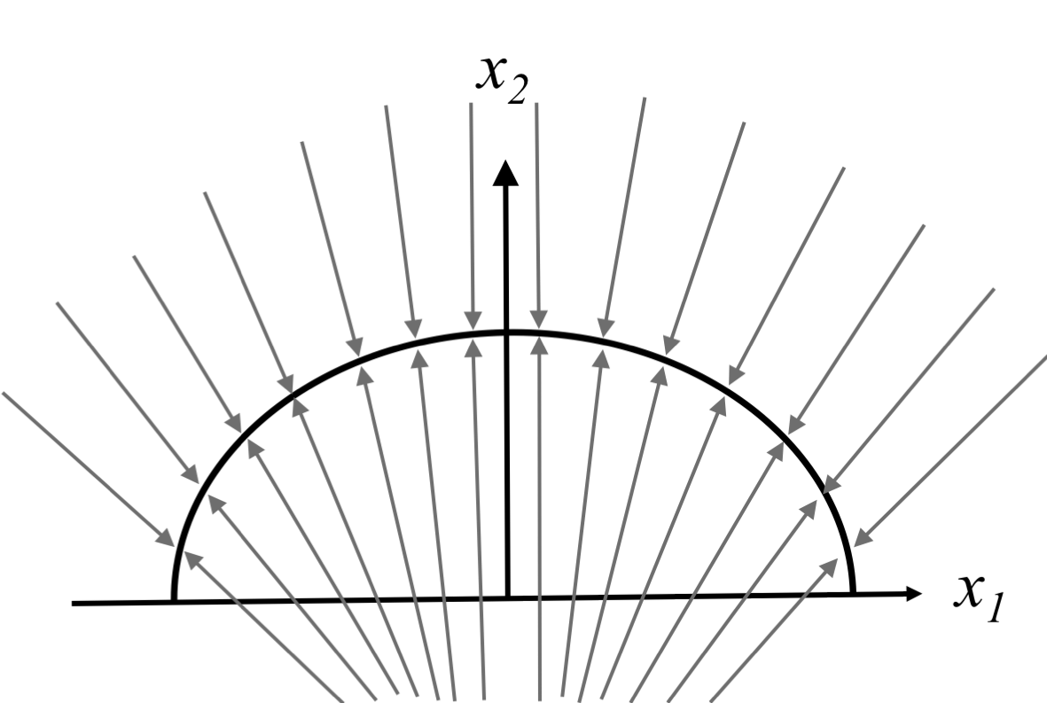
Usually, a sigmoid or ReLU function is used as the activation function. These activation functions are constructed using linear and flat domains. On the basis of these properties of activation functions, maps the input subspace related to the linear domain of the activation function to a one-dimensional space to align the vector . If the number of sharing the same input subspace is , the defines a -dimensional sub-hyperplane. The DNN models the data distribution by continuously pasting these sub-hyperplanes as if they were the tangent spaces of a data manifold. That is, the DNN embeds the input space in the output space by pasting the sub-hyperplanes and compresses the tangent direction of these sub-hyperplanes (Fig. 1). Deeper and more complex DNNs can be understood as a collection of such three-layer DNN. Thus, such deeper DNNs can model more complex manifold structures as a combination of simple manifold structures modeled by a three-layer DNN Basri and Jacobs (2017). Note that the output of a three-layer DNN, a part of the deeper DNN, is referred to as a hidden layer. This is only one example of how a DNN models a data manifold. However, many studies have suggested that there are resemble property in successful trained DNNs Irie and Kawato (1990); Hinton and Salakhutdinov (2006); Brahma et al. (2016); Basri and Jacobs (2017); Rifai et al. (2011); Mototake and Ikegami (2015). By replacing the input space from x to , we can also model a time-series data manifold using DNN.
In this study, using a trained DNN that models a time-series data manifold , we propose a method of extracting information about the symmetry of a dynamical system. As described later in Sec. V, our proposed framework does not require special DNNs, so we can directly utilize the vast knowledge obtained from studies on physical data analysis using DNNs. This is why we select the DNN from multiple machine learning models that can be used to model manifolds.
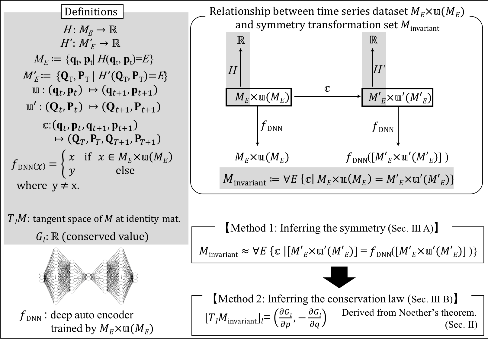
III Method
In this section, we describe our proposed framework for estimating the conservation law from a time-series dataset of dynamics. The schematic diagram of the proposed framework is shown in Fig. 2. The framework consists of two methods. In Sec. III.1, on the basis of the derivation of the relationship between the symmetry of the time-series dataset distribution and the conservation law (Sec. II), we propose a method of inferring the symmetry of data manifold using the Monte Carlo sampling method. In Sec. III.2, we describe the proposed method of inferring the conservation law from the obtained symmetry.
III.1 Method 1: Inferring the symmetry of data manifold using Monte Carlo sampling method
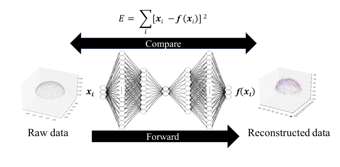
In this subsection, we propose a general method of inferring the symmetric property of data manifolds, which is not limited to the physical time-series dataset. It can be inferred from the discussion in Sec. II.5 that data points that are not on the manifold in the input space are attracted to the manifold (Fig. 1). Once the data points are attracted to the manifold in the hidden layer, they continue to exist on the manifold in the output . We propose a method based on this property of DNNs for extracting the symmetry of the data manifold using a deep autoencoder Hinton and Salakhutdinov (2006). The deep autoencoder is a model that compresses the input space to a low-dimensional hidden layer and decompresses the layer to an output space with the same dimension as the input space. In the decompression process, only the subspace of the input space around the data manifold is recovered because of the DNN property. On the basis of this property, we can evaluate whether a transformation causes the dataset distribution to remain in the same subspace of the data manifold (Fig. 3). The procedure is as follows. First, we train the deep autoencoder using as a training dataset. Second, we input the transformed dataset into the trained deep autoencoder. Note that the deep autoencoder is not trained on the transformed dataset. Third, we evaluate the transformation using the mean squared error between the input distribution of the dataset and its mapped distribution:
| (40) |
A smaller value implies that is a more invariant transformation. Using the criterion , we approximate the invariant transformation set as
| (41) |
To infer the conservation law, it is necessary to estimate the invariant transformation set of the manifold . The invariant transformation set is defined as
| (42) |
In Eq. (40), by substituting for and for the transformation , we can approximate as
| (43) |
where dataset is generated from dynamics data at energy . The approximated invariant transformation set is obtained approximately by sampling from the probabilistic density:
| (44) |
where is set as small as necessary and is a normalization constant. Note that to actually perform this sampling, it is necessary to first give a concrete coordinate system of in which physicists want to search conservation laws.
As mentioned in Sec. II.1, continuous symmetries form a Lie group. Using the continuous parameter set , we define the representation of the Lie group as a -dimensional matrix , where is the degree of freedom of the target Hamiltonian system. is a continuous parameter set, and . In the following, candidate invariant transformations are searched for within the Lie group representations. The invariant transformation is obtained by sampling an element of the matrix following the probability distribution
| (45) |
To perform this sampling, we need to specify . Ideally, should be set to . However, it is necessary to set to an appropriate finite value because errors are included in the time-series dataset and the training results of DNN. Such affected by noise cannot be set in advance. In addition, the target distributions in this study are assumed to be the global flat minima, because the same surface following the invariant transformation exists. Generally, such a target distribution needs an enormous amount of time to sample. Therefore, in this study, we use the replica-exchange Monte Carlo (REMC) method Hukushima and Nemoto (1996) as a sampling method to overcome these problems. Such a method enables us to perform efficient sampling by parallel sampling with different noise intensities of while exchanging noise intensities with each other. In the state of a large noise, we can realize global sampling from the abstract distribution
| (46) |
where . By exchanging this sampling information with the state of a small noise, we can perform efficient sampling from the target distribution . The detailed explanation of REMC method and the setting parameters of the method are described in Appendix E, and the target is determined by analyzing the sampling results as described in Appendix F. The procedure of Method 1 is summarized in Algorithm 1.
Note that there is no description of how to train a DNN in this study. In the training of the deep autoencoder, the number of nodes in the hidden layer is an important hyperparameter. On the other hand, since this is a quantity that determines how much the phenomenon is to be reduced, it is considered to be provided by the physicist.
III.2 Method 2: Inferring the conservation law from obtained symmetry
From the sampling results in Sec. III.1, we propose a method of estimating the infinitesimal transformation, which represents the invariance of the Hamiltonian and the equation of motion.
The set of invariant transformation is characterized by the -dimensional continuous parameter . Therefore, is a -dimensional differential manifold. Note that forms a Lie group as we mentioned in Sec. II.1. The infinitesimal transformation is estimated as the tangent vector of at . Using , we estimate as
| (47) |
By serializing the transformation matrix , we define the vector
| (48) |
where . The implicit function representation of the manifold is defined as
| (49) |
In the representation of the implicit function, the infinitesimal transformation is estimated as the tangent vector of the manifold at the position
| (50) |
where and is the representation of the identity matrix I in the space. We estimate this tangent space from the sampling results obtained in Sec. III.1.
The Jacobian matrix of for parameters of the subset , , is defined as . If the Jacobian matrix at becomes nonsingular, from the implicit function theorem, variables other than , , can be expressed as . This implies that, around , the implicit equations in Eq. (49) representing the manifold can be decomposed into the following simultaneous equations:
| (51) |
where corresponds to the continuous parameter of the continuous transformation . Differentiating these equations with respect to around a point yields simultaneous partial differential equations,
| (52) |
Solving these simultaneous partial differential equations gives the tangent vector of the manifold around . Using the tangent vector as the nonserialized representation , we can estimate an infinitesimal transformation as
| (53) |
Thus, the invariant transformation is obtained as the tangent vector of the manifold at point . Therefore, if can be regressed around as the first-order polynomial of , the conservation law can be inferred without approximation. Compared with the Hamiltonian estimation and conservation law estimation, this is the advantage of conservation law estimation, because, in general, the Hamiltonian estimation requires infinite-order polynomial approximation. On the other hand, the estimation accuracy of the tangent space from finite data with noise is often low. In this study, we propose a method of estimating the infinitesimal transform with high accuracy by using all sampled transformation data, not only data around . Another way to avoid this problem is also discussed in Sec. V.
The simultaneous equations in Eq. (LABEL:simul_eq) can be estimated by the following procedure. First, the upper limit of the dimension of the manifold is estimated by applying principal component analysis and the “elbow” method to as described in Ulfarsson and Solo (2008). Alternatively, the approximate dimension of can be estimated by using the manifold dimension estimation method such as the method described in Levina and Bickel (2005). Using such an estimated dimension of , we can prepare candidate dimension . Second, we extract one variable set . By orthogonal distance regression Brown and Fuller (1990), we regress to a -order implicit polynomial function,
| (54) |
where is the regression coefficient, and is a binary vector indicating whether the basis is selected. The indicator vector and the dimension of the manifold are determined by a model selection method, such as the Bayesian information criterion (BIC) Schwarz (1978). To select the model, it is necessary to estimate the likelihood. The method of estimating the likelihood is described in Appendix G. If , can be determined by visualization. Note that, unlike the estimation of the tangent space , the upper limit of the order of polynomial function must be sufficiently large because the entire sampling data is regressed. This regression and model selection is performed for all ; then, an implicit function representation of can be obtained.
From the obtained simultaneous equations, we obtain the simultaneous differential equations. If the Jacobian matrix is singular, the solution of the simultaneous equations diverges or becomes indefinite. In that case, the variable set is extracted again and the same procedure is repeated. If the Jacobian matrix is nonsingular, we can obtain the infinitesimal transformation according to Eq. (53). In this method, by narrowing down the regressing area of to the neighborhood of , we obtain a higher accurate estimation of infinitesimal transformation with a lower-order polynomial function in Eq. (54).
IV Results
We evaluate the proposed method using one geometrical structure and three physical systems: (i) a half sphere, (ii) constant-velocity linear motion, (iii) a two-dimensional central force system, and (iv) a collective motion system. Case (i) has a rotational symmetry. In case (i), we confirm that Method 1 can obtain a set of transformations corresponding to the symmetry. Cases (ii) and (iii) are systems that conserve the momentum and angular momentum, respectively. Using these cases, we verified Method 2. Finally, we apply both proposed methods to (iv), which is a complicated collective motion system, and attempted to infer the collective coordinate and conservation law. In each case, the parameters of DNN are set as described in Appendix H, and REMC are set as described in Appendix E.
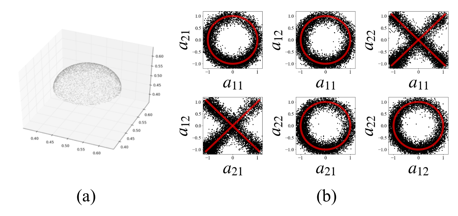
(i) Half sphere
The dataset of case (i) was generated by the function
| (55) |
where was set to be . We generated 1,671 samples according to Eq. (55). The dataset of case (i) [shown in Fig. 4(a)] was used to verify the ability of Method 1 described in Sec. III.1, which extracts the symmetry. We set the coordinate system as and limit the transformation on the - plane. In such a case, the transformation matrix is defined as
| (56) |
In this coordinate system, the half sphere has a rotation symmetry and a mirror symmetry. The rotation symmetry transformation is represented as
| (57) |
where is a rotation angle, and the mirror symmetry transformation is represented as
| (58) |
where is an angle of the mirror plane with the axis. The mirror symmetry is a discrete symmetry; therefore, the invariant transformation of the half sphere is represented as , where and
| (59) | |||||
| (62) | |||||
| (63) |
By comparing Eq. (56) with Eqs. (59) and (62), we obtain the implicit function representation of the invariant transformation as
| (64) |
Method 1 was applied to such a system.
The sampling results of are shown in Fig. 4(b) as black dots. In the figures, the red curves were fitted by the selected implicit polynomial functions using the BIC. The fitting results are
| (65) |
where we determine to be 1 by visualizing the distribution of .
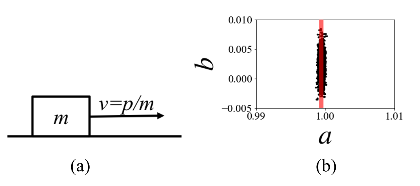
(ii) Constant-velocity linear motion
The dataset of case (ii) was generated using the one-dimensional Hamiltonian system
| (66) |
where was set to be . We generated 1,000 samples by solving Eq. (66). In this case, we show that the proposed method can infer the momentum conservation law. We set the coordinate system as . In such a coordinate system, and are related as . This means that and have the same coordinate transformation. Thus, the transformation matrix is defined as
| (67) |
As a result, two parameters and must be sampled. The sampling results of are shown in Fig. 5 as black dots and the red curves were fitted by the selected implicit polynomial function using the BIC. The fitting result is
| (68) |
The simultaneous partial differential equations in Eq. (52), where , were obtained from the fitting results. From the solution of the simultaneous partial differential equations, we obtained the infinitesimal transformation
| (69) |
where we determined to be by visualizing the distribution of . By substituting this Eq. (69) into Eq. (1) and solving the equations, we estimated the conserved value as . This result shows that the momentum was conserved.
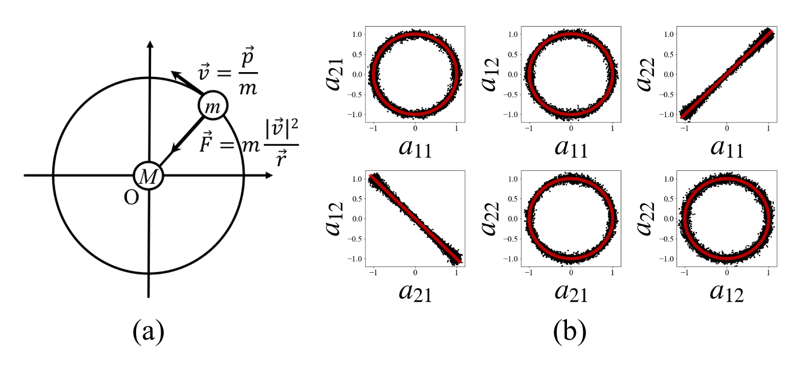
(iii) Two-dimensional central force system
The dataset of case (iii) was generated using the Hamiltonian system
| (70) |
where , , and , , and were set to be 1. We generated 1,000 samples by solving Eq. (70). We set the coordinate system as . In such a coordinate system, and are related as . Thus, and have the same coordinate transformation, and the transformation matrix is defined as
| (71) |
As a result, only four parameters must be sampled.
In the canonical dynamics of , it is impossible to transform one orbit to another with the same energy but different long-axis radii using the linear transformation in Eq. (71). Therefore, the invariant transformation for can be represented as a product of invariant transformation for subspace for specific energy and long-axis radii. This implies that the invariant transformation set for certain energy and certain long-axis radii must include some invariant transformations for . On the basis of this property of the Hamilton system of , we apply the proposed method only to the time-series dataset of a circular orbit with radius 1.
The sampling results of are shown in Fig. 6 as black dots and the red curve in each figure was fitted by the selected polynomial function using the BIC. The fitting results are
| (72) |
where we determine to be by visualizing the distribution of . The simultaneous partial differential equations in Eq. (52), where , were obtained from the fitting results. By solving the simultaneous partial differential equations, we obtained the infinitesimal transformation
| (77) | |||||
| (82) | |||||
| (87) |
where the values in the final formula are to one decimal place. By substituting Eqs. (82) and (87) into Eq. (1) and solving the equation, we estimated the conserved value as . This result shows that the angular momentum was conserved.
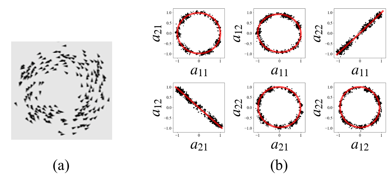
(iv) Collective motion system
In this case, we apply our framework to an -body collective motion system called the Reynolds boid model Reynolds (1987). In this model, each individual moves following three forces, which are the force attracting each other, separating each other, and aligning the orientation of each other:
| (88) | |||||
| (89) |
where , , and , represent the index of an individual. The attraction, separation, and alignment terms are represented by the first, second, and third terms in Eq. (88), and each force has the interaction range, , , , and angle of view, , , , respectively. The parameters , , , , , , , , and of the Reynolds boid model can be tuned to simulate the collective motion of living things such as birds or fish Reynolds (1987); Couzin et al. (2002). In this study, we focused on a parameter set that simulates the torus-type behavior of a school of fish in the sea. Such a torus-type collective motion can be realized in a two-dimensional space. Therefore, we set the dimension to two in this study. By solving Eq. (88), we generated 2,000 steps of time-series data of the torus-type collective motion by 200 individuals.
To infer the conservation law of collective motion, we need to set a candidate collective coordinate. In this study, we set the collective coordinate on the basis of the following considerations. First, from the visual symmetry of the motion, the average position and average momentum of all particles over time are set as the origin of the coordinate system. Second, since the same behavior is observed regardless of the individual, each individual is considered to have no degree of freedom. From these considerations, we set the coordinate system as , and prepared the dataset as
| (90) | |||||
| (91) |
where , , and represents all combinations of individuals and time steps . We randomly selected 5,000 samples from this dataset for the training of DNN. Then, the transformation matrix is defined as
| (92) |
The sampling results of are shown in Fig. 7(b) as black dots and the red curves fitted by the selected implicit polynomial functions using the BIC. The fitting results of the selected implicit polynomial functions are
| (93) |
where we determine by visualizing the distribution of . The simultaneous partial differential equations in Eq. (7), where , were obtained from the fitting results. By solving the simultaneous equations, we obtained the infinitesimal transformation
| (98) | |||||
| (103) | |||||
| (108) |
where the values in the final formula are to one decimal place. By substituting Eqs. (103) and (108) into Eq. (1) and solving the equation, the conserved value was estimated as . This result shows that the angular momentum was conserved.
V Summary and Discussion
From the results of case (i), we confirm that Method 1 could be used to extract the symmetry. The results of cases (ii) and (iii), wherein the expected conservation laws were inferred, show that Method 2 is effective. By comparing cases (i) and (iii), we observe differences in the selected implicit polynomial functions in the - and - spaces. These differences emerged from the mirror symmetry in case (i). This finding supports the assertion that the method works well in extracting the symmetry of a system. For a more practical collective motion system [i.e., case (iv)], we inferred the angular momentum conservation law; the results thereof are consistent with a previous study Couzin et al. (2002). In the previous study, it is suggested that angular momentum is conserved in torus-type swarming patterns. Additionally, the finding of a conservation law in the collective coordinates, where the degree of freedom of an individual was degenerated and the origin of the coordinates is the average position and momentum of the swarm, suggests that a dynamical system with a large degree of freedom can be reduced to a central force dynamical system.
The present study deals only with the case of a single conservation law. If there are multiple conservation laws, the dimension of the manifold becomes increase. In such a case, Eq. (52) has multiple orthogonal solutions. Theoretically, the proposed method can still handle such a problem, but the number of combinations of polynomial regressions [Eq. (54)] increases exponentially, and the Jacobian matrix is more likely to be singular. Therefore, it is necessary to develop a more efficient method of estimating an infinitesimal transformation. To estimate an infinitesimal transformation, one needs only to estimate a tangent space around the identity element. As there is a finite sample, in the proposed method, the manifold formed by Lie groups is regressed over the entire space. It is expected that the tangent space can be directly estimated by orthogonal basis decomposition by introducing various constraints.
In this study, we used the deep autoencoder to model the time-series data manifolds; nonetheless, there is no need to use the deep autoencoder. The only requirement for a machine learning model is that it has a mapping function that can determine whether it is on or outside the manifold. From this perspective, the deep autoencoder can be replaced with another type of DNN model, such as a variational autoencoder Kingma and Welling (2013) or a generative adversarial network Goodfellow et al. (2014). Additionally, a feed-forward-type DNN, which is widely used in DNN research, can be used in our proposed method by additionally training a neural network that reconstructs the input data from the output layer of the feed forward neural network. The same method should be feasible for use with machine learning models that have mapping functions that embed data manifolds into the output space (e.g., the kernel method). Thus, the proposed framework can potentially extract interpretable physical knowledge from the wide range of machine learning models. Note that the structure of the extracted manifold changes depending on the DNN model and its training settings. This is because the reduced model acquired inside the DNN changes depending on the DNN model and the training settings. How to learn time-series dataset using a certain DNN model and training settings are understood as the implicit construction of the reduced model.
In this study, we showed that the proposed framework can infer the hidden conservation laws of a complex system from DNNs that have been trained with physical data of the system. On the basis of the obtained results, it is expected that the knowledge of physical data embedded in the trained DNNs in previous studies and the knowledge of physicists can be merged. This should accelerate the research on the construction of reduced models.
Acknowledgements.
I would like to thank Dr. Y. Ando, Professor S. Goto, Dr. S. Takabe, Professor H. Hino, Professor K. Fukumizu, Professor K. Hukushima, Professor T. Ikegami, Professor K. Ishikawa, Mr. H. Yamashita, Professor Y. Yue, and Mr. K. Sakamoto for useful discussions. This work was supported by KAKENHI grant numbers JP17H01793 and JP19K12111.Appendix A Derivation of equivalent condition to make Hamiltonian invariant
The identity condition has the equivalent expression
| (109) |
This condition can be transformed to an equivalent conditional expression represented by a set,
| (110) |
which is proved in Appendix C. Replacing with the transformed parameters does not change the set: . Therefore, Eq. (110) is rewritten as
| (111) |
From the definition of the transformed Hamiltonian , are satisfied. By substituting these into Eq. (111), we obtain the target condition equivalent to the identity condition as
| (112) |
Appendix B Derivation of equivalent condition to make canonical equations invariant
The identity condition in Eq. (18),
| (113) |
has the equivalent expression
| (114) |
This condition can be transformed to the following equivalent conditional expression represented by a set:
| (115) | |||||
The proof of the equivalence of Eqs. (114) and (115) is a multivariable case of the proof described in Appendix C. By treating as a set of elements, we transform the condition in Eq. (115) to the equivalent condition (see the proof in Appendix D)
| (116) | |||||
Replacing with the transformed parameters does not change the set:
| (117) | |||||
| (118) |
Therefore, Eq. (116) is rewritten as
| (119) | |||||
From the definition of the transformed canonical equations [Eqs. (14) and (15)], we obtain
| (120) | |||||
| (121) |
By substituting this into Eq. (119), we obtain the target condition equivalent to the identity condition in Eq. (18) as
| (122) | |||||
Appendix C Proof of Eq. (109)Eq. (110) and Eq. (114)Eq. (115)
The problem can be abstracted as the proposition below:
| (123) |
where and are single-valued functions.
| (124) |
The contrapositive of (124) is . This contrapositive is proved as follows. Since , there exists and , which satisfy , but . Therefore, is satisfied because .
| (125) |
The contrapositive of (125) is . This contrapositive is proved as follows. Select one from , which satisfies and . Since is a single-valued function, is not included in the set of that satisfies . Thus, holds. Therefore, is satisfied.
Appendix D Proof of Eq. (115)Eq. (116)
The problem can be abstracted as the proposition below:
| (126) |
where and are single-valued functions.
| (127) |
The contrapositive of (127) is . This contrapositive is proved as follows. Since , there is a set of and , which satisfies and . Therefore, holds. It means that is satisfied.
| (128) |
The contrapositive of (128) is . This contrapositive is proved as follows. Since , there is a set of and , which satisfies and . Therefore, is satisfied.
Appendix E Replica exchange Monte Carlo (REMC) method and its parameters
Using , we re-express Eq. (45) as
| (129) |
The REMC method takes samples from the joint density
| (130) |
where and .
In the REMC method, sampling from the joint density is performed on the basis of the following updates.
-
1
Sampling from each density
Sampling from , where is the normalization constant. The sampling is performed by a conventional Monte Carlo method, such as the Metropolis–Hastings algorithm Hastings (1970).
-
2
Exchange between two densities corresponding to noise intensity
The exchanges between the configurations and correspond to adjacent inverse temperatures following the probability , where
Sampling from a distribution with a larger tends not to have a local minimum. Hence, sampling from the joint density overcomes the local minima in distributions with small and enables the rapid convergence of sampling.
In the execution of EMC sampling, we adopted the Metropolis–Hastings algorithm Hastings (1970) to sample each state of . When we performed the Metropolis–Hastings sampling, a candidate for the next sample is picked from the conditional probability distribution with precondition
| (131) |
where is set as
| (134) |
, , and in Eq. (134) are set as Table 1 for the evaluation of the proposed method in Sec. IV. In case (ii) constant-velocity linear-motion, the sampling parameters of and in Eq. (67) were set as different values [The values are described as ( of ) / ( of ) in the column of (ii) constant-velocity of Table 1]. Each state of was determined following the exponential function Nagata and Watanabe (2008):
| (137) |
where is set as root-mean-square error (RMSE) for in trained DNN, because it represents the minimum value of . and are set as shown in Table 1 for each case.
| Parameter name | (i) Half sphere | (ii) Constant-velocity | (iii) Central force | (iv) Collective motion |
|---|---|---|---|---|
| Sampling size | 10,000 | 10,000 | 10,000 | 10,000 |
| L | 20 | 30 | 30 | 30 |
| 1.4 | 1.9 | 1.4 | 1.4 | |
| 3.0 | 0.03 / 0.3 | 0.3 | 0.3 | |
| 0.6 | 0.7 | 0.8 | 0.8 | |
| 5.0 | 1.0 | 5.0 | 5.0 | |
| 4.42 | 5.41 | 1.67 | 8.0 | |
| Burn-in length | 1.000 | 10,000 | 1,000 | 10,000 |
| Selected noise intensity | 8.66 | 5.41 | 3.45 | 71.3 |
Appendix F Noise intensity of sampling
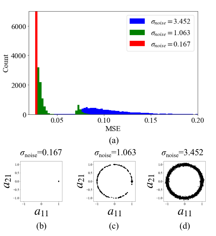
Depending on the difference in , the sampling results corresponding to low MSE and the sampling results corresponding to high MSE are obtained [Fig. 8(a)]. In the low-MSE region, the transformation matrix corresponding to the identity matrix is sampled [Fig. 8(b)]. In the high-MSE region, the transformation matrix corresponding to the rotation matrix is sampled [Fig. 8(d)]. At intermediate noise intensities, sampling between both conditions is achieved [Fig. 8(c)]. On the basis of such a structure, in this research, we select the noise intensity that realizes the non-identity transformation such as of Fig. 8. For the evaluation of the proposed method in Sec. IV, we select the noise intensity for each evaluation case as shown in Table 1.
Appendix G Estimation of likelihood for the model selection
Under the assumption that samples of transformation are given with Gaussian noise, the following likelihood is defined for a statistical selection of implicit function.
| (138) | |||||
| (139) | |||||
| (140) | |||||
| (141) |
where is the minimum distance from a data point to a subspace defined by the implicit function . The normalized constant is estimated numerically as the Riemann sum.
Appendix H DNN model and its training parameters
| Parameter name | (i) Half sphere | (ii) Constant-velocity | (iii) Central force | (iv) Collective motion |
|---|---|---|---|---|
| Training datasize | 1,671 | 1,000 | 1,000 | 5,000 |
| Network structure | 3-10-2-10-3 | 4-10-1-10-4 | 8-20-1-20-8 | 8-20-1-20-8 |
| Activation function | sigmoid | tanh | sigmoid | sigmoid |
| Training algorithm | Adam | Adam | Adam | Adam |
| Training iteration | 50,000 | 100,000 | 50,000 | 50,000 |
| Minibatch size | 10 | 30 | 10 | 10 |
| Library | theano Bastien et al. (2012); Bergstra et al. (2010) | scikit-learn Pedregosa et al. (2011) | theano | theano |
In this section, we describe the DNN models and their training settings.
In this study, we used deep autoencoders as DNN models. In all cases (i), (ii), (iii), and (iv), the DNNs consisted of an input layer, three hidden layers, and an output layer. The number of nodes in each layer was set as shown in the “Network structure” in Table 2.
The activation functions of the deep autoencoders were set as the sigmoid or hyperbolic tangent functions as shown in the “Activation function” in Table 2. The sigmoid function is defined as
| (142) |
and the tanh function is defined as
| (143) |
The numbers of samples used for training DNN are shown in Table 2 as “Training datasize ”. The Adam method Kingma and Ba (2014) was used for training. The training iterations are shown in Table 2. In the training, the data were divided into minibatches whose sizes are shown in Table 2 as “Minibatch size”.
References
- Tomonaga (1950) S. Tomonaga, Prog. Theor. Phys. 5, 544 (1950).
- Bohm and Pines (1951) D. Bohm and D. Pines, Phys. Rev. 82, 625 (1951).
- Pines and Bohm (1952) D. Pines and D. Bohm, Phys. Rev. 85, 338 (1952).
- Tomonaga (1955) S. Tomonaga, Prog. Theor. Phys. 13, 467 (1955).
- Saffman (1992) P. G. Saffman, Vortex Dynamics (Cambridge University Press, Cambridge, 1992).
- Vicsek and Zafeiris (2012) T. Vicsek and A. Zafeiris, Phys. Rep. 517, 71 (2012).
- Ikegami et al. (2017) T. Ikegami, Y. Mototake, S. Kobori, M. Oka, and Y. Hashimoto, Philosophical Transactions of the Royal Society A: Mathematical, Physical and Engineering Sciences 375, 20160351 (2017).
- Schmidt and Lipson (2009) M. Schmidt and H. Lipson, Science 324, 81 (2009).
- Greydanus et al. (2019) S. Greydanus, M. Dzamba, and J. Yosinski (Curran Associates, Inc., 2019) pp. 15353–15363.
- Toth et al. (2019) P. Toth, D. J. Rezende, A. Jaegle, S. Racanière, A. Botev, and I. Higgins, arXiv preprint arXiv:1909.13789 (2019).
- Bondesan and Lamacraft (2019) R. Bondesan and A. Lamacraft, arXiv preprint arXiv:1906.04645 (2019).
- Gibbs (1876) J. W. Gibbs, Transactions of the Connecticut Academy of Arts and Sciences 3, 108 (1875–1876).
- Gibbs (1878) J. W. Gibbs, Transactions of the Connecticut Academy of Arts and Sciences 3, 343 (1877–1878).
- Irie and Kawato (1990) B. Irie and M. Kawato, Transactions of the Institute of Electronics, Information and Communication Engineers D 73, 1173 (1990).
- Hinton and Salakhutdinov (2006) G. E. Hinton and R. R. Salakhutdinov, Science 313, 504 (2006).
- Brahma et al. (2016) P. P. Brahma, D. Wu, and Y. She, IEEE Transactions on Neural Networks and Learning Systems 27, 1997 (2016).
- Basri and Jacobs (2017) R. Basri and D. W. Jacobs, in 5th International Conference on Learning Representations, ICLR 2017, Toulon, France, April 24-26, 2017, Conference Track Proceedings (OpenReview.net, 2017).
- Rifai et al. (2011) S. Rifai, Y. N. Dauphin, P. Vincent, Y. Bengio, and X. Muller, in Advances in Neural Information Processing Systems 24, edited by J. Shawe-Taylor, R. S. Zemel, P. L. Bartlett, F. Pereira, and K. Q. Weinberger (Curran Associates, Inc., 2011) pp. 2294–2302.
- Mototake and Ikegami (2015) Y. Mototake and T. Ikegami, International Symposium on Artificial Life and Robotics (2015).
- Yeo (2017) K. Yeo, arXiv preprint arXiv:1710.01693 (2017).
- Morton et al. (2018) J. Morton, A. Jameson, M. J. Kochenderfer, and F. Witherden, in Advances in Neural Information Processing Systems 31, edited by S. Bengio, H. Wallach, H. Larochelle, K. Grauman, N. Cesa-Bianchi, and R. Garnett (Curran Associates, Inc., 2018) pp. 9258–9268.
- Rudy et al. (2018) S. H. Rudy, J. N. Kutz, and S. L. Brunton, arXiv preprint arXiv:1808.02578 (2018).
- Takeishi et al. (2017) N. Takeishi, Y. Kawahara, and T. Yairi, in Advances in Neural Information Processing Systems 30, edited by I. Guyon, U. V. Luxburg, S. Bengio, H. Wallach, R. Fergus, S. Vishwanathan, and R. Garnett (Curran Associates, Inc., 2017) pp. 1130–1140.
- Lusch et al. (2018) B. Lusch, J. N. Kutz, and S. L. Brunton, Nature Communications 9, 4950 (2018).
- Ohtsuki and Ohtsuki (2016) T. Ohtsuki and T. Ohtsuki, J. Phys. Soc. Jpn. 85, 123706 (2016).
- Ohtsuki and Ohtsuki (2017) T. Ohtsuki and T. Ohtsuki, J. Phys. Soc. Jpn. 86, 044708 (2017).
- Broecker et al. (2017) P. Broecker, J. Carrasquilla, R. G. Melko, and S. Trebst, Scientific Reports 7, 8823 (2017).
- Ch’Ng et al. (2017) K. Ch’Ng, J. Carrasquilla, R. G. Melko, and E. Khatami, Phys. Rev. X 7, 031038 (2017).
- Carrasquilla and Melko (2017) J. Carrasquilla and R. G. Melko, Nature Physics 13, 431 (2017).
- Tanaka and Tomiya (2017) A. Tanaka and A. Tomiya, J. Phys. Soc. Jpn. 86, 063001 (2017).
- Saito and Kato (2017) H. Saito and M. Kato, J. Phys. Soc. Jpn. 87, 014001 (2017).
- Van Nieuwenburg et al. (2017) E. P. Van Nieuwenburg, Y.-H. Liu, and S. D. Huber, Nature Physics 13, 435 (2017).
- Zhang et al. (2018) P. Zhang, H. Shen, and H. Zhai, Phys. Rev. Lett. 120, 066401 (2018).
- Noether (1918) A. Noether, Math. Phys. KI II 235 (1918).
- Reynolds (1987) C. W. Reynolds, in Proceedings of the 14th Annual Conference on Computer Graphics and Interactive Techniques, SIGGRAPH ’87 (Association for Computing Machinery, New York, NY, USA, 1987) p. 25–34.
- Struckmeier and Riedel (2002) J. Struckmeier and C. Riedel, Annalen der Physik 11, 15 (2002).
- Hukushima and Nemoto (1996) K. Hukushima and K. Nemoto, J. Phys. Soc. Jpn. 65, 1604 (1996).
- Ulfarsson and Solo (2008) M. O. Ulfarsson and V. Solo, IEEE Transactions on Signal Processing 56, 5804 (2008).
- Levina and Bickel (2005) E. Levina and P. J. Bickel, in Advances in Neural Information Processing Systems 17, edited by L. K. Saul, Y. Weiss, and L. Bottou (MIT Press, 2005) pp. 777–784.
- Brown and Fuller (1990) P. J. Brown and W. A. Fuller, Statistical analysis of measurement error models and applications: Proceedings of the AMS-IMS-SIAM Joint Summer Research Conference held on June 10-16, 1989, with support from the National Science Foundation and the US Army Research Office, Vol. 112 (American Mathematical Soc., 1990).
- Schwarz (1978) G. Schwarz, Annals of Statistics 6, 461 (1978).
- Couzin et al. (2002) I. D. Couzin, J. Krause, R. James, G. D. Ruxton, and N. R. Franks, Journal of Theoretical Biology 218, 1 (2002).
- Kingma and Welling (2013) D. P. Kingma and M. Welling, arXiv preprint arXiv:1312.6114 (2013).
- Goodfellow et al. (2014) I. Goodfellow, J. Pouget-Abadie, M. Mirza, B. Xu, D. Warde-Farley, S. Ozair, A. Courville, and Y. Bengio, in Advances in Neural Information Processing Systems 27, edited by Z. Ghahramani, M. Welling, C. Cortes, N. D. Lawrence, and K. Q. Weinberger (Curran Associates, Inc., 2014) pp. 2672–2680.
- Hastings (1970) W. K. Hastings, Biometrika 57, 97 (1970).
- Nagata and Watanabe (2008) K. Nagata and S. Watanabe, Neural Networks 21, 980 (2008).
- Bastien et al. (2012) F. Bastien, P. Lamblin, R. Pascanu, J. Bergstra, I. J. Goodfellow, A. Bergeron, N. Bouchard, and Y. Bengio, “Theano: new features and speed improvements,” Deep Learning and Unsupervised Feature Learning NIPS 2012 Workshop (2012).
- Bergstra et al. (2010) J. Bergstra, O. Breuleux, F. Bastien, P. Lamblin, R. Pascanu, G. Desjardins, J. Turian, D. Warde-Farley, and Y. Bengio, in Proceedings of the Python for Scientific Computing Conference (SciPy) (2010) oral Presentation.
- Pedregosa et al. (2011) F. Pedregosa, G. Varoquaux, A. Gramfort, V. Michel, B. Thirion, O. Grisel, M. Blondel, P. Prettenhofer, R. Weiss, V. Dubourg, J. Vanderplas, A. Passos, D. Cournapeau, M. Brucher, M. Perrot, and E. Duchesnay, Journal of Machine Learning Research 12, 2825 (2011).
- Kingma and Ba (2014) D. P. Kingma and J. Ba, arXiv preprint arXiv:1412.6980 (2014).