Nested Column Generation decomposition for solving
the Routing and Spectrum Allocation problem
in Elastic Optical Networks

Abstract

With the continued growth of Internet traffic, and the scarcity of the optical spectrum, there is a continuous need to optimize the usage of this resource. In the process of provisioning elastic optical networks using the flexible frequency grid paradigm, telecommunication operators must deal with a combinatorial optimization problem that is NP-complete namely the Routing and Spectrum Allocation (RSA) problem.

Following on our previous study, where we used Integer Linear Programming, and proposed a Column Generation algorithm based on a Lightpath decomposition, which proved to be the most efficient so far, we now consider the traditional Configuration decomposition that has been studied in other works in the past. In the process, we created an new mathematical model using two variable sets instead of a single variable set. Equally important, we independently rediscovered the Nested Column Generation technique, and we used it to propose an algorithm that led to a considerable improvement on the previous algorithms that use the same Configuration decomposition. When compared to the latest such existing study, our algorithm achieved an accuracy gap of 1% as opposed to 14.3% for the previous study, and a running time two orders of magnitude faster on average.

1 Introduction

The core networks of Internet (called also long-haul networks) are based on optical technology and their links are made of optical fibers. As a way to increase the capacity, these networks implement Wavelength Division Multiplexing (WDM), where the idea is to transmit data simultaneously at multiple carrier optical frequencies. Traditionally, the multiplexing was done according to a Coarse WDM frequency grid (called fixed grid) where the carrier wavelength granularity is 50 GHz. As of 2012, the International Telecommunication Union issued a new recommendation that defines a flexible Dense WDM frequency grid with a finer frequency granularity of 12.5 GHz called a frequency slot [IUT, 2012]. This evolution has allowed the emergence of Elastic Optical Networks.

The main phase in the process of designing an Elastic Optical Network is concerned with traffic provisioning, which consists of assigning a routing path, and allocating an optical spectrum range to each traffic demand. The spectrum range corresponds to a number of contiguous frequency slots. This provisioning problem is called the Routing and Spectrum Allocation (RSA) problem.

The RSA optimization problem has been shown to be NP-hard by Shirazipourazad et al. [2013]. Among the existing algorithms, heuristics are in general fast but they do not provide any guarantee on the quality of the solutions. Therefore, in order to solve it exactly (i.e., with a calculated accuracy), we need to employ Integer Linear Programming (ILP). While ILP compact formulations (e.g., link-based) have a polynomial number of variables, they do not scale well when the problem instances reach a real-life size. Therefore, we consider decomposition formulations.

1.1 Existing studies

Various mathematical models have already been proposed for solving the RSA problem, including several column generation models, however with different decomposition schemes, and different solution processes. All classical ILP models are not scalable and can only solve very small data instances, i.e., with few nodes and with a spectrum made of a very limited number of slices.

Ruiz et al. [2013] proposed a first column generation model, with the minimization of the number of denied demands and the amount of non-served bit-rate. They are able to solve data instances with up to 96 slots, and an overall demand distributed over a set of 180 node pairs in the Spain network (21 nodes).

Klinkowski et al. [2014] improved the previous formulation with the use of valid inequalities (cuts), but did not go significantly farther.

Klinkowski & Walkowiak [2015] reformulated the RSA problem as a mixed-integer program and solved it using a branch-and-price algorithm. In order to enhance the performance of their algorithm, a simulated annealing-based heuristic was added.

In a recent attempt to exactly solve large-size instances of RSA problem, Klinkowski et al. [2016] proposed a branch-and-price algorithm. However, the resulting algorithm is not an exact algorithm and the Linear Program (LP) value is not a valid bound to assess the quality of the ILP solutions, as the authors use pre-computed lightpaths, and did not consider all possible lightpaths.

In our previous study [Enoch & Jaumard, 2018], we proposed an ILP formulation based on a Lightpath decomposition, and we solved it using Column Generation technique. This Lightpath decomposition proved to be very efficient compared to previous algorithms. But, as we scaled up our problem instances, we sensed the limits of its efficiency. In fact, the fine-granularity of the Lightpath decomposition makes it that the final ILP in the Column Generation process contains a very high number of columns, and can take very long to be solved. Consequently, we decided to explore a different decomposition based on a column definition as a set of lightpaths referred to as a Configuration of lightpaths.

The Configuration decomposition has been previously explored in [Jaumard & Daryalal, 2016] using Column Generation and combining two algorithms to solve the Pricing Problem, one of which is a Path-based ILP that is restricted to a pre-computed subset of paths and generates feasible Configurations quickly, and the other one is an optimal Link-based ILP used at the end of Column Generation to guarantee the optimality of the Pricing Problem. However, this solution suffers from two issues. The pre-computation for the Path-based Pricing Problem is complex, and the Link-based Pricing Problem is inefficient.

In the current study, we introduced a new formulation for the Configuration decomposition, and more importantly, we independently rediscovered the Nested Column Generation technique that expands on the traditional Column Generation approach. The inspiration behind the Nested Column Generation technique was to have only one Path-based ILP for the Pricing Problem, and solve it optimally and efficiently, which leads to an overall efficient algorithm.

Throughout this document, we use the following acronyms to refer to different algorithms:

• L_CG refers to the Column Generation algorithm using a Lightpath decomposition introduced by the same author of this work in [Enoch & Jaumard, 2018];

• C_CG refers to a Column Generation algorithm using a Configuration decomposition introduced by Jaumard & Daryalal [2016];

• C_NCG refers to the new Nested Column Generation algorithm using a Configuration decomposition introduced in this work;

2 RSA Decomposition Model

2.1 Statement of the RSA Problem

We consider an Elastic Optical Network and we represent its topology by an undirected graph $G=(V,L)$ with node set $V$ and link set $L$. The bandwidth spectrum of the optical network is sliced into a set $S$ of frequency slots of width 12.5GHz. The traffic is defined by a set $K$ of optical connections where each connection $k\in K$ is defined by a source $s_{k}$, a destination $d_{k}$ and a bandwidth demand $D_{k}$, expressed in terms of a number of slots.

Given an Elastic Optical Network, and a traffic demand matrix between its nodes, the RSA problem consists of finding optical channels for the traffic requests, as to maximize the overall throughput. For a given traffic request $k\in K$ from source node $s_{k}$ to destination node $d_{k}$, with spectrum demand $D_{k}$, an optical channel (or lightpath) is a combination of a routing path $\Pi_{k}$ from node $s_{k}$ to node $d_{k}$, and an optical slice that is composed of a contiguous set of spectrum slots and that is continuous throughout the routing path $\Pi_{k}$. An optical slice is - by definition - a contiguous set of frequency slots, thus it can be characterized (in addition to its width $D_{k}$) by its low-end spectrum slot which we refer to as a starting slot.

2.2 Decomposition Model

The ILP model is based on a Configuration decomposition. We define a Configuration as a set of link-disjoint lightpaths provisioning distinct requests and having the same starting slot. Figure 1 shows an example of a Configuration of three lightpaths.

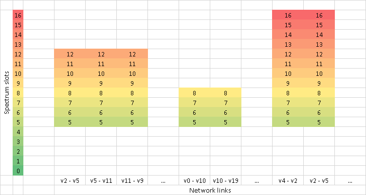
Figure 1: Configuration illustration - The first request connects node-pair $\{v_{2},v_{9}\}$. It is routed using three links. Its demand is 8 slots. This configuration contains three lightpaths all of which start at slot 5.

We have experimented with the mathematical model proposed in [Jaumard & Daryalal, 2016], but we observed that it performed poorly both in terms of the quality of the solution, and in terms of the computation time. The intuition behind this is that the Configuration columns are relatively large which makes LP relaxation take longer to converge to its optimal value ($z_{LP}^{\star}{}$). This also leads to a high contention among the Configurations during the ILP Branch-and-Bound phase, which produces an integral solution (${\tilde{z}}_{ILP}{}$) with a relatively large accuracy gap.

Therefore, we created a new mathematical model that employs two sets of variables instead of only one, and that proved to be easier to solve.

Let $C$ be the set of all possible Configurations. Each Configuration $c\in C$ is defined with the help of the following parameters:

• $a_{k}^{c}$: indicates if a request $k$ is provisioned by Configuration $c$.

• $b_{\ell}^{sc}$: indicates if one of the requests provisioned in Configuration $c$ is routed on link $\ell$ while assigned slot $s$ as part of its spectrum slice.

The two sets of decision variables are as follows:

• $z_{c}$ is a binary variable that indicates if Configuration $c$ is selected in the solution.

• $y_{k}$ is an intermediate binary variable that indicates if a request $k$ is granted in the solution, and can be expressed in terms of $z_{c}$ as follows:

  $$y_{k}=\sum_{c\in C}a_{k}^{c}z_{c}\qquad k\in K.$$ (1)

The objective function consists of maximizing the throughput and is written in terms of $y_{k}$ as follows:

$$z\quad=\quad\max\quad\sum_{k\in K}D_{k}y_{k}$$ (2)

subject to:

$$y_{k}\leq\sum_{c\in C}a_{k}^{c}z_{c}\qquad k\in K,$$ (3)

$$\sum_{c\in C}b_{\ell}^{sc}z_{c}\leq 1\qquad \ell\in L,s\in S,$$ (4)

$$z_{c}\in\{0,1\}\qquad c\in C,$$ (5)

$$0\leq y_{k}\leq 1\qquad k\in K.$$ (6)

Constraints (3) means that a request $k$ is granted only if it is provisioned in at least one of the Configurations $z_{c}$. Constraints (4) make sure that each slot on each fiber link is not used by more than one Configuration $z_{c}$. The integrality of variables $y_{k}$ is guaranteed by the combination of (2) and (3), and needs not to be explicitly enforced in (6).

This mathematical model uses a set of intermediate variables $y_{k}$ which translates into relaxing the upper-bound demand constraints in [Jaumard & Daryalal, 2016]. In fact, the constraints (3) are a relaxation of the definition (1). As a consequence of this relaxation, the two-variable-sets model requires to post-process the Configurations in the final solution, as to remove the extra provisioning that violates the demand constraints and to re-establish the equality (1).

Additionally, we have experimented with a model where the intermediate variables are aggregated per node-pair ($y_{sd}=\sum_{c\in C}a_{sd}^{c}z_{c}$) such that their number can be lesser. This prospect was unfruitful because the variables $y_{sd}$ then had to be integer (whereas the variables $y_{k}$ are binary), thus having a loose domain, which impacts the tightness of the model negatively.

In the next sections, we describe the Nested Column Generation technique and the solution design and we present the results of the model defined above with intermediate binary variables $y_{k}$. Prior to that, we present In the sequel of this section a discussion about a possible extension of the mathematical model.

2.3 Guard-band Extension of the RSA Problem

When provisioning traffic demand in an Elastic Optical Network, a guard band of one slot is reserved on top of the spectrum slice of each request.

If we consider the case where traffic requests are not aggregated, this means that if there are multiple requests for the same node pair, these requests can be provisioned independently, thus, eventually taking different routing paths, and using spectrum slices that are not neighbors. If such requests happen to be routed on the same path using neighbors spectrum slices, they need not to be separated by a guard-band.

In order to account for this possibility, we extend our model as follows:

Given a node pair $w=\{u,v\}$, let $K_{w}=\{k_{1},k_{2},...,k_{n}\}$ be the set of requests between u and v. We will refer to these requests as atomic. For $m\in\{1,2,...,n\}$, we denote ${K^{\prime}}_{w}^{m}$ the set of combinations of m requests from $K_{w}$. We have

$$|{K^{\prime}}_{w}^{m}|=\binom{n}{m}.$$ (7)

This quantity is the $m^{th}$ binomial coefficient for power $n$. Let ${K^{\prime}}_{w}=\cup_{m=1}^{m=n}\>{K^{\prime}}_{w}^{m}$. We have

$$|{K^{\prime}}_{w}|=\sum_{m=1}^{m=n}\binom{n}{m}=2^{n}-1.$$ (8)

Each combination of atomic requests produces a new derived request by summing up their demands. ${K^{\prime}}_{w}$ is referred to as the set of derived requests. Note that $K_{w}\subset{K^{\prime}}_{w}$ given that $K_{w}={K^{\prime}}_{w}^{1}$. The derived requests obtained for $m\in\{2,...,n\}$ are referred to as composite requests. Let $K^{\prime}=\cup_{w\in W}{K^{\prime}}_{w}$. If a request $k^{\prime}$ is derived from an atomic request $k$, we note $k^{\prime}\leftarrow k$.

For each node pair, we enumerate the derived requests using a binomial tree as in Figure 2. Given this data structure’s properties, this operation is done recursively as we go through the atomic requests of a given node pair. For each derived request, we keep track of the atomic requests used in its making.

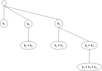
Figure 2: A binomial tree of order n = 3 for a node pair with 3 atomic requests

In order to account for all possible derived requests, the ILP model is slightly modified as follows, such that only the first set of constraints is impacted:

$$z\quad=\quad\max\quad\sum_{k\in K}D_{k}y_{k}$$ (9)

subject to:

$$y_{k}\leq\sum_{c\in C}\sum_{k^{\prime}\leftarrow k}a_{k^{\prime}}^{c}z_{c}\qquad k\in K,$$ (10)

$$\sum_{c\in C}b_{\ell}^{sc}z_{c}\leq 1\qquad \ell\in L,s\in S,$$ (11)

$$z_{c}\in\{0,1\}\qquad c\in C,$$ (12)

$$0\leq y_{k}\leq 1\qquad k\in K.$$ (13)

This modification means that the Pricing Problem needs to include all the derived requests. As calculated earlier, the number of derived requests is much larger than the number of atomic requests. Therefore, while this extension offers an elegant way to account for non-aggregated connections and saving on the optical spectrum guard-band, by enumerating derived requests, it remains unscalable for a practical dataset such as the one introduced in [Enoch & Jaumard, 2018], and therefore, it is presented for its theoretical value and is not implemented in this study.

3 Nested Column Generation

Column Generation consists of decomposing the original problem into a Restricted Master Problem (RMP), i.e., with a restricted number of variables, and one or several Pricing Problems (PP). The RMP and the PP(s) are solved alternately. Solving the RMP consists in selecting the best columns, while solving one PP allows the generation of an improving potential column, i.e., a column such that, if added to the current RMP, improves the optimal value of its LP relaxation. The process continues until the optimality condition is satisfied, i.e., the so-called reduced cost that defines the objective function of the Pricing Problems is non-positive for all of them [Chvatal, 1983]. The optimal value of the linear relaxation of the so-obtained RMP is denoted by $z_{LP}^{\star}$ and represents an upper-bound on the optimal solution of the RSA problem. After the Column Generation phase, the next step consists of solving the ILP model associated with the last RMP, which produces an integral solution with a value, denoted as ${\tilde{z}}_{ILP}$, which represents a lower-bound on the optimal solution of the RSA problem. The integral solution thus-obtained is said to be $\varepsilon$-optimal where $\varepsilon$ denotes the relative difference between the two bounds: $\quad\varepsilon=(z_{LP}^{\star}-{\tilde{z}}_{ILP})/z_{LP}^{\star}$.

Considering the Configuration decomposition in [Jaumard & Daryalal, 2016], although Column Generation is a powerful technique, we observed that the link-based formulation of the Pricing Problem was not efficient enough. Given that the Pricing Problems need to be solved at each iteration of Column Generation, their performance can be an important hindrance to the over-all efficiency. In order to address this difficulty, we devised an algorithm based on the idea of solving the Pricing Problem itself using Column Generation, which approach we referred to as Nested Column Generation, and which we realized that it has been employed in other optimization problems in the vast area of Operations Research.

3.1 Existing Nested Decompositions

The idea of applying recursive decomposition was suggested by Dantzig [1963]. Some of the first generic implementations for Integer Linear Programming go back to the early 70’s such as Glassey [1973] and Ho & Manne [1974]. Subsequently, many implementations for Integer Linear Programming have been produced.

Vanderbeck [2001] implemented a nested decomposition approach to a cutting-stock problem. First the author devises a subproblem that generates cutting patterns and solves it using Column Generation, in turn, with the help of another subproblem that generates sections. The author notes that the cutting-pattern generation subproblem is only solved approximately given that Column Generation only produces lower and upper bounds on the minimum reduced cost of a cutting-pattern, and uses the lower bounds on the reduced costs to produce a Lagrangian bound on the cutting problem. The author recognizes that this is a ”heuristic based on the tools of exact optimization”, given that the optimality of the Lagrangian bound is not guaranteed.

Hennig et al. [2012] proposed a Nested Column Generation algorithm for the Crude Oil Tanker Routing and Scheduling problem such that the first subproblem generates a cargo-route for each ship. This subproblem is solved using a Branch-and-Price algorithm with the help of a second-level subproblem which generates a route for each ship.

Closer to the applications in optical networks, Vignac et al. [2016] presented multiple models for the Grooming, Routing and Wavelength Assignment problem, among which, a Column Generation algorithm where a subproblem for each wavelength is defined to find the traffic carried by this wavelength, called a Wavelength Routing Configuration. This subproblem is itself decomposed into arc-disjoint grooming-patterns, thus leading to a nested decomposition. Similarly to Vanderbeck [2001], the bounds of the Pricing Problems are used to compute Lagrangian dual bounds on the master LP, thus resulting into a heuristic.

Caprara et al. [2016] referred to Nested Column Generation as Recursive Dantzig-Wolfe Reformulation and used this approach to design a Branch-and-Price algorithm for solving the Temporal Knapsack Problem.

Tilk et al. [2019] proposed an algorithm for solving the Vehicle Routing Problem with Multiple Resource Inter-dependencies where both the Master Problem and the Pricing Problem are solved using Branch-and-Price. The authors also give a detailed review on the use of nested decompositions in other publications (e.g., Cordeau et al. [2001], Dohn & Mason [2013]).

3.2 Processing Flow

Figure 3 shows the processing flow of our Nested Column Generation algorithm as applied to the RSA problem. The Column Generation flow used to solve the Pricing problem, is identical to that used to solve the Master problem, thus the naming of Nested Column Generation.

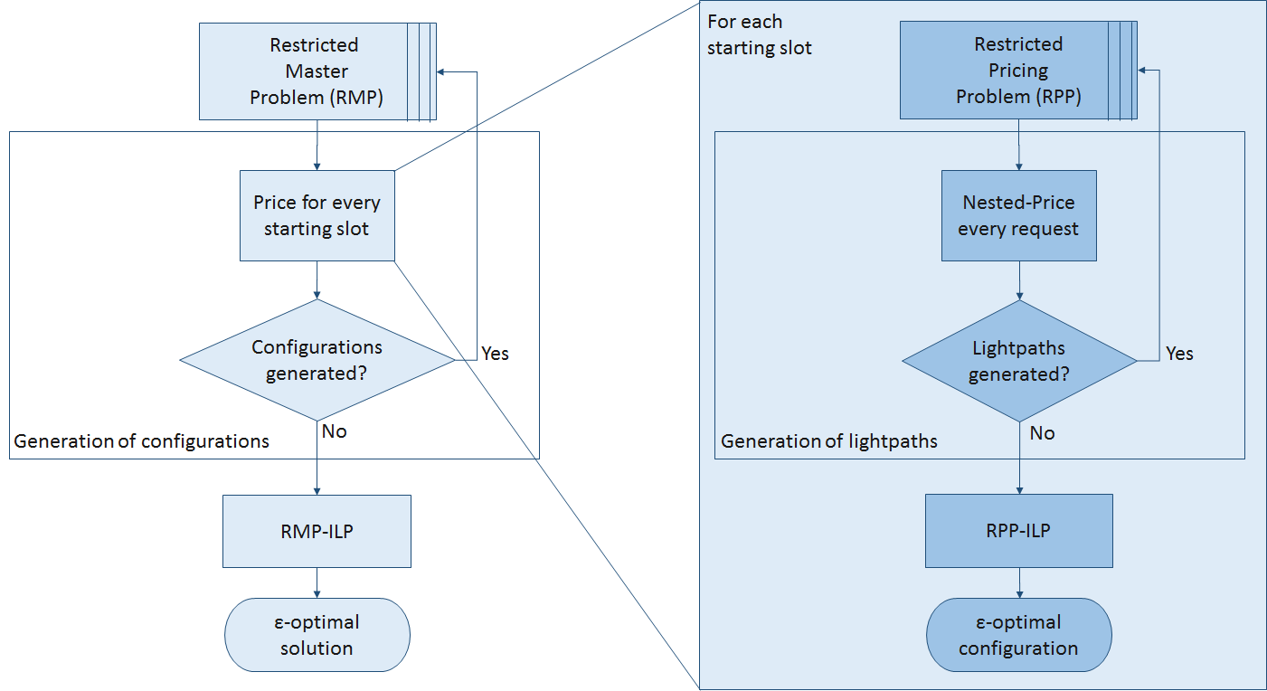
Figure 3: Nested Column Generation Flow for RSA

The stop condition for the generation of Configurations for the Master Problem is met when, after considering all the starting slots of the optical spectrum, the Pricing Problem cannot produce any improving Configurations, i.e., the optimal value of the ILP associated with the Pricing Problem is null ( $rc^{\star}_{ILP}=0$).

3.3 Discussion about the optimality of the Linear Relaxation of the RMP

The main outcome of Column Generation is to produce a strong linear relaxation bound $z_{LP}^{\star}{}$ on the optimal solution of the Master Problem. This outcome is based on the premise that the Pricing Problem is solved to optimality [Dantzig, 1963], in particular, when the stopping condition to exit Column Generation is verified ($rc^{\star}_{ILP}=0$). However, in Nested Column Generation, the Pricing Problem is solved using Column Generation meaning that the integer solutions that we obtain for the Pricing Problems are only lower-bounds (assuming Branch-and-Price is not employed as is the case in this study).

Nevertheless, thanks to Nested Column Generation, we have also an upper bound on the optimal solution of the Pricing Problem ($rc_{LP}^{\star}$). So when the Pricing Problem fails to generate a new Configuration (${\tilde{rc}}_{ILP}=0$), there are two possibilities:

• $rc_{LP}^{\star}=0$: we can deduce that $rc^{\star}_{ILP}=0$, and therefore the exit condition is satisfied. In this case, the LP relaxation of the Master Problem is optimal.

• $rc_{LP}^{\star}>0$: this means there is no guarantee that $rc^{\star}_{ILP}=0$, and therefore, the LP relaxation of the Master Problem might not be optimal.

To sum up, theoretically Nested Column Generation does not guarantee the accuracy of the LP relaxation bound of the Master Problem. In fact, some studies resorted to a Branch-and-Price approach (with additional overhead) for solving the Pricing Problem in order to guarantee this accuracy [Hennig et al., 2012, Caprara et al., 2016, Tilk et al., 2019]. However, it is possible empirically to conclude whether the LP relaxation is optimal or not by verifying if the Pricing Problem was solved to optimality in the last iteration.

4 Solution Design

4.1 Pricing Problem

As shown in Figure 3, the goal of the Pricing Problem is to compute an optimal Configuration for each starting slot $s$ (for clear distinction from the starting slot, we will index the provisioning slots by $s^{\prime}$). In this section we also drop the Configuration index $c$ in order to alleviate the notation.

Given that the starting slot is fixed for each Pricing Problem, the optical slice allocated to any request $k$ can be deduced from the starting slot and the size of the request demand $D_{k}$. Therefore each Pricing Problem needs only to produce the routing paths for the lightpaths of the optimal Configuration. Let $\Pi_{k}$ be the set of all possible routing paths of request $k$. A routing path $\pi\in\Pi_{k}$ of request $k$ is defined with the help of a binary parameter $\delta_{\pi}^{\ell}$ that indicates if link ${\ell}$ is part of the routing path $\pi$.

We define a set of decision variables for the Pricing Problem as follows:

• $\beta_{\pi}$ is a binary variable that indicates if routing path $\pi$ is included in the the optimal Configuration.

Let $\mu_{k}{}$ and $\mu_{\ell s^{\prime}}{}$ be the dual values of constraints (3) and (4) respectively. The reduced cost for the model (2)-(6) is:

$$rc\quad=\quad\max\qquad\sum_{k\in K}\mu_{k}a_{k}-\sum_{\ell\in L}\sum_{s^{\prime}\in S}\mu_{\ell s^{\prime}}b_{\ell}^{s^{\prime}}.$$ (14)

The correspondence between the pricing solution and the master’s parameters is as follows:

$$a_{k}=\sum_{\pi\in\Pi_{k}}\beta_{\pi} k\in K$$ (15)

$$b_{\ell}^{s^{\prime}}=0 \ell\in L,s^{\prime}\notin\{s,\dots,s+D_{k}^{s}-1\}$$ (16)

$$b_{\ell}^{s^{\prime}}=\sum_{k\in K}\sum_{\pi\in\Pi_{k}}\delta_{\pi}^{\ell}\beta_{\pi} \ell\in L,s^{\prime}\in\{s,\dots,s+D_{k}^{s}-1\}.$$ (17)

Therefore, for a given starting slot $s$, the pricing problem reads as follows:

$$rc\quad=\quad\max\sum_{k\in K}\sum_{\pi\in\Pi_{k}}\left(\mu_{k}-\sum_{\ell\in L}(\sum_{s^{\prime}=s}^{s+D_{k}^{s}-1}\mu_{\ell s^{\prime}})\delta_{\pi}^{\ell}\right)\beta_{\pi}$$ (18)

subject to:

$$\sum_{\pi\in\Pi_{k}}\beta_{\pi}\leq 1 k\in K$$ (19)

$$\sum_{k\in K}\sum_{\pi\in\Pi_{k}}\delta_{\pi}^{\ell}\beta_{\pi}\leq 1 \ell\in L$$ (20)

$$\beta_{\pi}\in\{0,1\} k\in K,\pi\in\Pi_{k}.$$ (21)

Constraints (19) mean that each request is provisioned at most once, and constraints (20) mean that each link is traversed by at most one lightpath. This ensures that the lightpaths forming the Configuration are link-disjoint.

4.2 Lightpath Generator

Let $\nu_{k}$ and $\nu_{\ell}$ be the values of the dual variables associated with constraints (19) and (20) respectively. Given a starting slot and given a request $k\in K$, the reduced cost is:

$$\max\quad\mu_{k}-\sum_{\ell\in L}(\sum_{s^{\prime}=s}^{s+D_{k}^{s}-1}\mu_{\ell s^{\prime}})\delta^{\ell}-\nu_{k}-\sum_{\ell\in L}\nu_{\ell}\delta^{\ell}$$ (22)

which we streamline as:

$$\max\qquad(\mu_{k}-\nu_{k})-\sum_{\ell\in L}\left((\sum_{s^{\prime}=s}^{s+D_{k}^{s}-1}\mu_{\ell s^{\prime}})+\nu_{\ell}\right)\delta^{\ell}$$ (23)

We get a shortest-path problem with non-negative weights for each $k\in K$:

$$\min\qquad\sum_{\ell\in L}\left((\sum_{s^{\prime}=s}^{s+D_{k}^{s}-1}\mu_{\ell s^{\prime}})+\nu_{\ell}\right)\delta^{\ell}.$$ (24)

5 Empirical Study

The datasets used in this empirical study use the Spain network topology with 21 nodes and 35 links, and the USA network topology with 24 nodes and 43 links.

The solution was implemented in Java. For the Branch-and-Bound part we used IBM Cplex solver 12.6 in a single thread mode. Shortest path calculation was done with an open-source Java library JGraphT implementing Dijkstra’s algorithm. The results were produced on a 3.6-4.0 GHz 4-core machine with 32 GB of memory.

Throughout the LP phase, only the columns in the basis are retained, and the columns that drop from the basis are dropped from the current RMP, as suggested by Dantzig [1963], in order to maintain the size of the LP manageable, and force the algorithm to produce better columns in terms of low-fractionality.

It is known that linear programs’ solvers (Cplex in this paper) induce some very small numerical errors. For being so small, usually these errors are not a big hindrance in Column Generation algorithms. But in this study, these errors can be quite a problem. In fact, at the second level of our Nested Column Generation, the lightpath generator is not solved as a linear program but is solved as an undirected graph shortest-path problem using Dijkstra which does not allow negative link weights. But, while all dual values in this paper are supposed to be non-negative, Cplex produces for some of them small negative values. In order to overcome this issue, we are rounding up to zero those negative dual values used in the link weights.

We observe for all the data instances that: When the Pricing Problems fail to generate new Configurations (i.e., ${\tilde{rc}}_{ILP}=0$), we have also $rc_{LP}^{\star}=0$, which implies that $rc^{\star}_{ILP}=0$ meaning that the Pricing Problems are solved optimally. Therefore, the LP relaxation of the Master Problem $z_{LP}^{\star}$ is optimal and is indeed an upper-bound on the optimal solution $z^{\star}_{ILP}$ (see discussion at Section 3.3).

5.1 ICTON’16 dataset

This dataset was first introduced in [Jaumard & Daryalal, 2016] at the conference ICTON’2016, where it was solved using a Column Generation algorithm based on a Configuration decomposition which we refer to as C_CG. This dataset was generated using the Spain network topology. Table 1 shows the results obtained using the current algorithm as well as a comparison with the results published in [Jaumard & Daryalal, 2016] and the results published in [Enoch & Jaumard, 2018].

Table 1: ICTON’16 dataset - Solution and Comparison

Traffic demand			Solution quality			$\epsilon$ (%) comparison			CPU comparison (sec)
Offered load (Tbps)	|D|	|S|	$z_{LP}^{\star}$ (Tbps)	${\tilde{z}}_{ILP}$ (Tbps)	GoS (%)	C_NCG	L_CG	C_CG	C_NCG	L_CG	C_CG
Spain network: demand granularities in {1, 2,, 8} slots, i.e., {25, 50, …, 200} Gbps
3.7	35	50	3.7	3.6	98.0	2.8	0.0	14.0	0.5	0.3	50.0
4.8	45	60	4.8	4.7	98.9	1.1	0.0	13.0	0.6	0.4	86.0
6.8	60	75	6.8	6.72	99.3	0.7	0.0	15.0	0.8	0.7	147.0
7.5	64	85	7.5	7.15	96.0	4.9	0.0	19.0	0.8	1.3	176.0
7.4	70	100	7.4	7.32	99.3	0.7	0.0	16.0	1.2	1.7	263.0
9.7	80	120	9.7	9.52	98.4	1.6	0.0	16.0	1.4	2.5	323.0
12.0	112	150	12.0	11.95	100.0	0.0	0.0	14.0	1.7	5.3	417.0
20.5	180	330	20.5	20.2	98.4	1.6	0.0	18.0	4.0	25.6	1606.0
Spain network: demand granularities in {2, 4,, 16} slots, i.e., {50, 100, …, 400} Gbps
7.5	35	80	7.5	7.4	99.3	0.7	0.0	10.0	0.8	0.9	134.0
9.8	45	110	9.8	9.7	99.5	0.5	0.0	10.0	0.9	2.0	177.0
10.7	60	156	10.7	10.65	99.5	0.5	0.0	12.0	0.9	3.1	261.0
15.5	64	170	15.5	15.5	100.0	0.0	0.0	16.0	1.4	4.7	630.0
15.1	70	236	15.1	15.1	100.0	0.0	0.0	13.0	1.4	7.8	1342.0
16.9	80	256	16.9	16.85	100.0	0.0	0.0	14.0	1.4	10.3	1419.0
Average						1.1	0.0	14.3	1.3	4.8	502.2

We did not re-implement the algorithm C_CG of Jaumard & Daryalal [2016] and the comparison is made with the results that were published by the authors of that algorithm. Considering that they produced their results on a 1.9-2.5GHz machine (in contrast with our 3.6-4.0GHz machine), it would be reasonable to divide their computation times by two for the purpose of the comparison (below) that remains approximate.

While the C_CG algorithm by Jaumard & Daryalal [2016] takes around 4 minutes on average, the new C_NCG algorithm takes only 1.3 seconds on average, beating even the L_CG algorithm by Enoch & Jaumard [2018] at around 5 seconds on average.

Regarding the quality of the solution, while the L_CG algorithm solves this dataset to optimality, the C_NCG algorithm produces a solution accuracy around 1% on average, which is still a lot better than the accuracy of the C_CG algorithm of 14.3%.

In the next subsection, we will examine a dataset that is supposed to be much harder, and shall be more challenging for the new C_NCG algorithm.

5.2 INOC’18 dataset

This dataset was first introduced in [Enoch & Jaumard, 2018], where it was solved using a Column Generation algorithm L_CG based on a Lightpath decomposition. This dataset was generated using both the Spain network and the USA network topologies according to the following specifications:

• Demands are drawn from granularities {4, 8, 16} in units of spectrum slots, with respective proportions {70%, 20%, 10%}, thus generating requests that are relatively large compared to those encountered in today’s networks, hence producing instances with relatively a high level of difficulty.

• Offered load is spread over all node pairs. Therefore, after aggregation, the number of requests given as input to our algorithm corresponds to the number of node pairs in the network.

In order to ease down the complexity of the algorithm and enhance its execution, we opted for the following strategies:

• Requests are aggregated per node-pair. This has the advantage of reducing the number of requests in the optimization problem and easing-down the solving process. Note that theoretically, if the problem is solved to optimality, this strategy would potentially produce a solution with a worse quality than if the requests were not aggregated.

• Given the large size of the instances of this dataset, the numerical accuracy of the LP solving becomes crucial in order for the Column Generation to converge. To that end, Cplex parameter NumericalEmphasis is turned on.

• We have noticed that the Integer Linear Program (ILP) phase can take a long time to cover the whole of the Branch-and-Bound tree, without improving by much the integral solution. Therefore we have chosen to pre-terminate the Branch-and-Bound by setting the Cplex parameter EpGap to $10^{-1}$.

• We allow multi-threading during the Branch-and-Bound phase with up to 8 threads.

• Before the Integer Linear Program (ILP) phase, we set Cplex parameter Advance to 0 in order to enable the standard pre-solving operations instead of using the basis produced by the last iteration of Column Generation as a starting point for the Branch-and-Bound.

Table 2 shows the complete results obtained using the current algorithm in terms of the $\epsilon$-optimal solution as well as the computation time. We observe that instances Spain90, USA80 and USA90 register a spike in the computation time as compared to the other instances. As we have discussed in [Enoch & Jaumard, 2018], this is due to the fact that $z_{LP}^{\star}{}$ is lesser than the offered load. Consequently, the Column Generation needs a considerably larger number of columns to reach the $z_{LP}^{\star}{}$, and spends a relatively long time producing those columns. This dataset has been purposefully designed to showcase this type of difficult instances.

Table 2: INOC’18 dataset - Algorithm Results and Performance

Dataset				Solution quality				CPU time (sec)
Instance	|S|	|D|	Load (Tbps)	$z_{LP}^{\star}$ (Tbps)	${\tilde{z}}_{ILP}$ (Tbps)	$\epsilon$ (%)	GoS (%)	LP	ILP	Total
Spain network: Demands in {4,8, 16} slots, i.e., {100, 200, 400} Gbps
Spain_50	400	413	50.2	50.2	42.6	17.8	84.9	30.5	0.3	31.0
Spain_60	400	495	60.0	60.0	47.2	27.1	78.7	113.6	0.2	114.1
Spain_70	400	578	70.2	70.2	52.3	34.2	74.5	177.0	1.0	178.2
Spain_80	400	660	80.0	80.0	55.5	44.1	69.4	254.1	2.2	256.6
Spain_90	400	743	90.2	86.9	56.0	55.1	62.1	1,756.9	940.1	2,697.7
USA network: Demands in {4,8, 16} slots, i.e., {100, 200, 400} Gbps
USA_50	400	413	50.2	50.2	41.4	21.3	82.5	27.8	0.5	28.4
USA_60	400	495	60.0	60.0	45.6	31.6	76.0	350.4	3.1	353.8
USA_70	400	578	70.2	70.2	49.9	40.7	71.1	495.4	3.1	498.9
USA_80	400	660	80.0	78.3	53.2	47.2	66.5	1,441.2	204.2	1,646.3
USA_90	400	743	90.2	85.7	56.0	53.0	62.1	1,977.5	417.0	2,395.3

Table 3 shows a comparison with the results published in [Enoch & Jaumard, 2018]. We can make the following observations:

Table 3: INOC’18 dataset - Solution and Performance Comparison

Dataset		Quality comparison						CPU comparison (sec)
		$z_{LP}^{\star}$ (Tbps)		${\tilde{z}}_{ILP}$ (Tbps)		$\epsilon$ (%)
Instance	Load (Tbps)	C_NCG	L_CG	C_NCG	L_CG	C_NCG	L_CG	C_NCG	L_CG
Spain_50	50.2	50.2	50.2	42.6	48.0	17.8	4.6	31.0	22.4
Spain_60	60.0	60.0	60.0	47.2	57.8	27.1	3.8	114.1	28.1
Spain_70	70.2	70.2	70.2	52.3	66.6	34.2	5.4	178.2	42.2
Spain_80	80.0	80.0	80.0	55.5	73.6	44.1	8.7	256.6	71.9
Spain_90	90.2	86.9	86.9	56.0	75.0	55.1	15.8	2,697.7	1,131.1
USA_50	50.2	50.2	50.2	41.4	46.9	21.3	7.0	28.4	29.4
USA_60	60.0	60.0	60.0	45.6	55.0	31.6	9.1	353.8	55.8
USA_70	70.2	70.2	70.2	49.9	63.0	40.7	9.9	498.9	108.4
USA_80	80.0	78.3	78.3	53.2	65.5	47.2	19.6	1,646.3	1,122.0
USA_90	90.2	85.7	85.7	56.0	72.4	53.0	18.4	2,395.3	1,532.0
Average						37.2	10.2	820.0	414.3

• The upper-bound $z_{LP}^{\star}{}$ produced by the two algorithms is the same. A theoretical study of this upper-bound could be considered in a future work.

• The integral solution found by C_NCG algorithm is less good than the one found by the L_CG algorithm and the accuracy gap is a lot larger. This is due to the fact that a Configuration column is a lot larger than a Lightpath column. Consequently, in the ILP phase, if the Configuration column has even a small overlapping with another column in the integral solution, it is rejected as a whole. To get an intuition of this phenomenon, we could make an analogy with the Knapsack problem. If we suppose that we have a fractional Knapsack solution and we want to get the integral solution from it: The smaller the items in the fractional solution, the lesser the contention among them, and the better the integral solution.

• The computation time of the C_NCG algorithm is less good than that of the L_CG algorithm (double on average). This is also due to the disparity of size of the columns in each decomposition. That said, the computation time of the C_NCG algorithm remains reasonable considering the level of difficulty of this dataset.

While the C_NCG algorithm is more scalable than the previous study, it can be inefficient in terms of solution quality for the largest data instances. We conclude that the algorithm L_CG, based on the Lightpath decomposition, presented in [Enoch & Jaumard, 2018] remains the most efficient in terms of both solution quality and scalability.

6 Conclusion

Considering the provisioning of Elastic Optical Networks, we focused on the Routing and Spectrum Allocation (RSA) problem. We aimed to explore ways to improve the latest results published for this problem in [Jaumard & Daryalal, 2016]. In doing so, we independently rediscovered the Nested Column Generation technique, which we used to design an ILP algorithm based on the Configuration decomposition. The motivation behind this approach is to tame the difficulty of the Pricing Problem thus improving the overall performance. Additionally, we presented for the first time a theoretical extension of the mathematical model, where we don’t assume that the connections are aggregated for each node pair, and we make savings on the optical spectrum guard-band. Our new approach based on Nested Column Generation produced solutions with an accuracy near optimal for the reference dataset and improved the computation time by a factor of two orders of magnitude on average as compared to the latest existing Configuration decomposition algorithm in [Jaumard & Daryalal, 2016], which is a considerable leap in efficiency. In addition to the reference dataset used in [Jaumard & Daryalal, 2016], we also produced results for the dataset used in [Enoch & Jaumard, 2018], consisting of problem instances considerably larger and more difficult to solve.

Equipped with the Nested Column Generation technique, we could consider increasing the scope of the RSA problem in the future by adding other dimensions that are useful for real-life implementations such as varying the modulation formats, or minimizing the number of optical re-generators needed in the optical network.

References

- Caprara et al. [2016] Caprara, A., Furini, F., Malaguti, E., & Traversi, E. (2016). Solving the temporal knapsack problem via recursive dantzig–wolfe reformulation. Information Processing Letters, 116, 379–386.
- Chvatal [1983] Chvatal, V. (1983). Linear Programming. Freeman.
- Cordeau et al. [2001] Cordeau, J.-F., Stojković, G., Soumis, F., & Desrosiers, J. (2001). Benders decomposition for simultaneous aircraft routing and crew scheduling. Transportation Science, 35, 375–388. URL: https://doi.org/10.1287/trsc.35.4.375.10432. doi:10.1287/trsc.35.4.375.10432. arXiv:https://doi.org/10.1287/trsc.35.4.375.10432.
- Dantzig [1963] Dantzig, G. (1963). Linear Programming and Extensions. Princeton: Princeton University Press.
- Dohn & Mason [2013] Dohn, A., & Mason, A. (2013). Branch-and-price for staff rostering: An efficient implementation using generic programming and nested column generation. European Journal of Operational Research, 230, 157 -- 169. URL: http://www.sciencedirect.com/science/article/pii/S0377221713002464. doi:https://doi.org/10.1016/j.ejor.2013.03.018.
- Enoch & Jaumard [2018] Enoch, J., & Jaumard, B. (2018). Towards optimal and scalable solution for routing and spectrum allocation. Electronic Notes in Discrete Mathematics, 64, 335 -- 344. URL: http://www.sciencedirect.com/science/article/pii/S1571065318300350. doi:https://doi.org/10.1016/j.endm.2018.02.008. 8th International Network Optimization Conference - INOC 2017.
- Glassey [1973] Glassey, C. R. (1973). Nested decomposition and multi-stage linear programs. Management Science, 20, 282--292.
- Hennig et al. [2012] Hennig, F., Nygreen, B., & Lübbecke, M. (2012). Nested column generation applied to the crude oil tanker routing and scheduling problem with split pickup and split delivery. Naval Research Logistics, 59, 298--310.
- Ho & Manne [1974] Ho, J. K., & Manne, A. S. (1974). Nested decomposition for dynamic models. Mathematical Programming, 6, 121--140.
- IUT [2012] IUT (2012). Spectral grids for WDM applications: DWDM frequency grid. White Paper.
- Jaumard & Daryalal [2016] Jaumard, B., & Daryalal, M. (2016). Scalable elastic optical path networking models. In International Conference on Transparent Optical Networks - ICTON (pp. 1--4).
- Klinkowski et al. [2014] Klinkowski, M., Pioro, M., Zotkiewicz, M., Ruiz, M., & Velasco, L. (2014). Valid inequalities for the routing and spectrum allocation problem in elastic optical networks. In International Conference on Transparent Optical Networks - ICTON (pp. 1--5).