A general formulation of time-optimal quantum control and optimality of singular protocols

Abstract

We present a general theoretical framework for finding the time-optimal unitary evolution of the quantum systems when the Hamiltonian is subject to arbitrary constraints. Quantum brachistochrone (QB) is such a framework based on the variational principle, whose drawback is that it deals with equality constraints only. While inequality constraints can be reduced to equality ones in some situations, there are situations where they cannot, especially when a drift field is present in the Hamiltonian. The drift which we cannot control appears in a wide range of systems. We first develop a framework based on Pontryagin’s maximum principle (MP) in order to deal with inequality constraints as well. The new framework contains QB as a special case, and their detailed correspondence is given. Second, using this framework, we discuss general relations among the drift, the singular controls, and the inequality constraints. The singular controls are those that satisfy MP trivially so as to cause a trouble in determining the optimal protocol. Third, to overcome this issue, we derive an additional necessary condition for a singular protocol to be optimal by applying the generalized Legendre-Clebsch condition. This condition in particular reveals the physical meaning of singular controls. Finally, we demonstrate how our framework and results work in some examples.

1 Introduction

Control of quantum systems is important both in applications and in fundamental physics. In applications, development of quantum control will help perform a variety of tasks in quantum technologies such as quantum computation and quantum cryptography. In the fundamental aspect, control theory can clarify the limitations on our abilities to complete a certain task in quantum mechanics and provides a way of understanding quantum mechanics from an engineering point of view. An important subject in this line is the time-optimal quantum control [1, 2], which realizes the desired unitary evolution in the least possible time. Time-optimal quantum control is useful in a variety of applications, in that it saves time cost and enables manipulations of quantum systems in short decoherence time. In fact, some studies aim to consider time-optimal quantum control for practical purposes, including efficient design of elementary gates and subroutines in quantum computation [3, 4], quantum error-correcting codes [5], and cooling of quantum systems [6, 7]. On the other hand, time-optimal quantum control gives the physically attainable minimal time in the fundamental sense to realize prescribed quantum evolutions. Such minimal time may also be an important tool to estimate the complexity of quantum computation [8, 9, 10].

There are many studies related to time-optimal or time-efficient quantum control. Khaneja et al [1, 2] and Zhang et al [11] discussed time-optimal control by using the Lie algebraic approach. They treated such situations that some unitary operations can be done instantaneously, which is a good approximation if the corresponding interactions are sufficiently large. Quantum brachistochrone (QB) is a general theory for time-optimal quantum control problems [12, 13, 14]. QB treats the situations where the system Hamiltonian can be changed under some equality constraints. Russell and Stepney [15, 17], and Brody and Meier [16] discuss geometric methods for deriving the time-optimal Hamiltonian in the presence of a drift field, which is a fixed, uncontrollable interaction. There are also many studies [18, 19, 20, 21, 22, 23] which focus on unitary operations on a qubit. Among the above-mentioned researches, QB may be able to serve as a standard theory for time-optimal control in quantum systems because of its generality and wide applicability, and may provide a unified understanding of the results from other studies. For example, we will see later that the results by Brody and Meier [16] can be shown in a simple manner by QB. One can obtain analytical optimal solutions of QB for low dimensional systems [12, 13]. Recently, experimental realizations of time-optimal quantum control based on QB started to appear [24].

However, there is a weakness in the present QB. It cannot treat problems with inequality constraints on the system Hamiltonian, which are natural in usual physical systems. The most important inequality constraint is the one that the system has a finite energy bandwidth, which is usually imposed by the bounded capability of the experimental apparatus. A previous study [25] shows that this inequality constraint is reduced to an equality one in certain situations. However, it is not always the case in a more general situation where a drift field is present. In fact, Ref. [26] shows an example of the time-optimal control problem in which the inequality constraint cannot be reduced to the equality one. Since we cannot apply the present QB to such problems, we need to extend QB theory. We also want to clarify in which situation inequality constraints reduce to equality ones.

In this paper, we present a more general time-optimal control theory in quantum systems, which can be applied to the problem with inequality constraints. Instead of directly extending the present QB formulation, we employ an alternative approach to get compatible results with QB. Our theory is based on Pontryagin’s maximum principle (MP), which is a non-traditional variational calculus for optimal control under equality and inequality constraints. In fact, MP has been applied in many studies [18, 19, 21, 22, 23, 26, 27, 28, 29] of time-optimal control in quantum systems. There, however, MP is usually applied after individual quantum control problems are cast in a standard form in classical control theory with real variables. We will apply MP to time-optimal quantum control in its general form so that we can discuss the structure of time-optimal quantum control itself and that we can solve individual problems more simply and directly.

For the system with drift fields, we have a special class of solution for MP, which satisfies the necessary conditions provided by MP in a trivial way. Such solutions are called singular controls [23, 27]. Although we cannot determine the optimal singular control uniquely from MP, we can derive additional conditions for the singular control to be optimal. This can be done by applying the generalized Legendre-Clebsch conditions [30]. We will demonstrate in some examples that the obtained conditions determine, or at least restrict, the form of singular optimal control. The conditions are useful not only in applications but also in the interpretation of the singular control. We will see that singular controls tend to make use of the drift field.

The paper is organized as follows. We first formulate the time-optimal control problem in quantum systems in Sec. 2. In Sec. 3, we review the theory of QB with some refinement and then explain some results derived from QB. We present a general framework for the time-optimal control in quantum systems by virtue of MP and clarify its relation to QB in Sec. 4. In Sec. 5, we show some conditions for an inequality constraint to be reduced into an equality one. In Sec. 6, we give the definition of singular controls and provide some additional necessary conditions for a singular control to be optimal. In Sec. 7, we discuss optimality of singular controls in some examples by applying the developed theory and necessary conditions. Section 8 is devoted to conclusion and discussions.

2 The problem

We consider the problem of finding the time-optimal control protocol that generates a desired unitary evolution of a quantum system in the least possible time. There, we can design the time dependence of the Hamiltonian so as to realize the desired evolution through the Schrödinger equation. The optimal control protocol largely depends on the form of available Hamiltonians, which is usually restricted due to the experimental or theoretical setting. In this section, we shall formulate the problem and introduce some notations.

Consider a physical system represented by an $N$-dimensional Hilbert space $\mathcal{H}$. The group of unitary operators on $\mathcal{H}$ is identified with the $N$-dimensional unitary group $\mathrm{U}(N)$ (via a choice of a basis on $\mathcal{H}$). We shall deal with the subgroup $\mathrm{SU}(N)$ instead of $\mathrm{U}(N)$, neglecting the global phase of unitary operator, which does not affect the observables. This is equivalent to think of the Hamiltonian $H$ as an element of $\mathfrak{su}(N)$, i.e. a traceless Hermitian operator. Here, $\mathfrak{su}(N)$ denotes the Lie algebra of $\mathrm{SU}(N)$ with the convention $\mathrm{SU}(N)=\exp(-i\,\mathfrak{su}(N))$. We will often introduce an orthonormal basis ${\left\{\tau_{j}\right\}}_{j=1}^{N^{2}-1}$ of $\mathfrak{su}(N)$ such that $\tr{\left[\tau_{i}\tau_{j}\right]}=2\delta_{ij}$. Any Hermitian operator $A$ is then expanded as $A=\sum_{j}a^{j}\tau_{j}$ with real coefficients $a^{j}$.

Let $\mathcal{A}\subset\mathfrak{su}(N)$ be the set of available Hamiltonians which are realizable under the given experimental or theoretical setup. We assume that $\mathcal{A}$ is time independent. The set $\mathcal{A}$ of available Hamiltonians is usually defined by equality and inequality constraints mathematically.

In these terms, the problem we want to solve is the following. Let $(U_{f},\mathcal{A})$ be a given pair, where $U_{f}\in\mathrm{SU}(N)$ is the target unitary operator and $\mathcal{A}\subset\mathfrak{su}(N)$ is the set of available Hamiltonians. Find the least time $T\geqslant 0$ and the control $H(t)\in\mathcal{A}$, $0\leqslant t\leqslant T$, such that $U(0)=1$ and $U(T)=U_{f}$, where the unitary operator $U(t)$ is driven by the Schrödinger equation

$$i\frac{\mathrm{d}}{\mathrm{d}t}U(t)=H(t)U(t).$$ (1)

We give a simplest example of the time-optimal control problem in a qubit system. We assume that a $z$-directional magnetic field is fixed and that we can manipulate a magnetic field in the $xy$ plane with the maximum magnitude $\Omega$. The Hamiltonian is given by

$$H(t)=\omega_{0}\sigma^{z}+u^{x}(t)\sigma^{x}+u^{y}(t)\sigma^{y},\quad(u^{x})^{2}+(u^{y})^{2}\leqslant\Omega^{2},$$ (2)

where $\omega_{0}$ is a real constant. Since this Hamiltonian can generate arbitrary unitary operator in $\mathrm{SU}(2)$ with suitable control variables $u^{x}(t)$ and $u^{y}(t)$, we can consider the time-optimal control for any $U_{f}\in\mathrm{SU}(2)$. In this case, we can write the set $\mathcal{A}$ of available Hamiltonians as

$$\mathcal{A}={\left\{\omega_{0}\sigma^{z}+H_{c}\;\middle|\;\tr{\left[H_{c}(t)\sigma^{z}\right]}=0,\;\frac{1}{2}\tr{\left[H_{c}(t)^{2}\right]}\leqslant\Omega^{2}\right\}}.$$ (3)

3 Quantum Brachistochrone

Quantum brachistochrone (QB) [12, 13, 14] is a theory of time-optimal control on quantum systems. In this section, we review QB theory but with a slightly different derivation, which might be simpler. The present derivation is convenient in establishing a general correspondence between QB and a theory based on MP given in the next section, where the latter can treat inequality constraints. We also discuss (in Sec. 3.4) some general results which are directly obtained from QB, including the solution of the quantum Zermelo navigation [15, 16, 17].

3.1 Formulation

We assume that the set $\mathcal{A}$ of available Hamiltonians is given by

$$\mathcal{A}={\left\{H\in\mathfrak{su}(N)\;\middle|\;f^{j}(H)=0,\,j=1,\dots,p\right\}},$$ (4)

where $f^{j}$ are real functions. Then we can formulate the time-optimality problem in the previous section as follows: Minimize the functional $T=\int_{0}^{T}dt\;1$ of the Hamiltonian $H(t)$ and the unitary operator $U(t)$ under constraints $f^{j}(H)=0$ and the Schrödinger equation (1). We employ the method of Lagrange multipliers and define an action,

$$S:=\int_{0}^{T}dt\;{\left(1+L_{S}+L_{C}\right)},$$ (5)

where

$$L_{S} :=\tr{\left[F(t){\left(i\dot{U}U^{\dagger}-H(t)\right)}\right]},$$ (6)

$$L_{C} :=\sum_{j}\lambda_{j}(t)f^{j}(H),$$ (7)

and $F(t)\in\mathfrak{su}(N)$ and $\lambda_{j}(t)\in\mathbb{R}\;(j=0,1,\dots,p)$ are Lagrange multipliers. In the present formulation, the main part of the integrand in the action (5) is simply 1 and the variation of the action $S$ is explicitly taken with respect to the final time $T$. In the previous derivation [12, 13, 14], the variation of the total time is expressed in an indirect manner which is similar to that used in variation of arc length in differential geometry or in general relativity. The term $L_{S}$ represents the constraints that $U(t)$ must be related to $H(t)$ by the Schrödinger equation. The term $L_{C}$ represents the equality constraints $f^{j}(H)=0$ imposed.

By the method of Lagrange multipliers, we need $\delta S=0$ under the variations with respect to $H(t),U(t),F(t),\lambda_{j}(t)$, and $T$. The condition that the final unitary operator $U(T)$ is not changed by the variations imposes a condition for $\delta T$. Namely, we have both $U(T)=U_{f}$ before taking the variations and $U(T+\delta T)+\delta U(T+\delta T)=U_{f}$ after taking the variations. Therefore, we require a condition at $t=T$,

$$\delta U(T)+\dot{U}(T)\delta T=0.$$ (8)

3.2 Result

The result from the variational principle above is as follows, while its derivation is given in the next subsection. If $H(t)$ is a time-optimal control, then there exist $\lambda_{j}(t)\in\mathbb{R}$ for $j=0,1,\dots,p$ such that the operator

$$F(t)=\sum_{j}\lambda_{j}(t)\frac{\partial f^{j}(H)}{\partial H},$$ (9)

satisfies the quantum brachistochrone equation

$$i\dot{F}(t)={\left[H(t),F(t)\right]},$$ (10)

and

$$\tr{\left[H(t)F(t)\right]}=1.$$ (11)

Therefore, we can obtain the time-optimal protocol $H(t)$ for $(U_{f},\mathcal{A})$ by solving the equations (9), (10), and (11) with the boundary conditions $U(0)=1$ and $U(T)=U_{f}$.

The statement above is the same as that of Ref. [13], except that eq. (11) is a new condition which arises in the present derivation. Note that this is only a condition for initial $H$ and $F$ because $\tr{\left[H(t)F(t)\right]}$ is constant in time by the QB equation (10). Moreover, because the overall scale of $F$ is arbitrary, eq. (11) essentially states that $\tr{\left[F(0)H(0)\right]}\neq 0$ and merely gives of a normalization of $F$.

We will discuss the role of the condition (11) in Sec. 5 and 6 from the viewpoint of the maximum principle, which leads to the same condition (29). Here, we shall just see how the condition (11) was interpreted in the previous studies [12, 13, 14, 24, 25]. Consider the Hamiltonian of the form $H(t)=H_{d}+H_{c}(t)$ with constraints $\tr[H_{c}^{2}]=\Omega$ and $H_{c}\in\mathcal{C}$, where $\Omega>0$ and $\mathcal{C}$ is a certain subspace of $\mathfrak{su}(N)$. This is a common class of constraints and was treated in the previous studies. Then, eq. (9) becomes $F(t)=\lambda(t)H_{c}(t)+F^{\prime}(t)$. When $H_{d}=0$, the condition (11) is equivalent to $\lambda\neq 0$, which was implicitly assumed in the previous studies. The condition (11) guarantees this implicit assumption. On the other hand, the case $H_{d}\neq 0$ allows the solutions with $\lambda=0$ in general. This correspond to a singular control, which will be defined and discussed in Sections 5 and 6.

Note that we can also consider the time-optimal control problem of state evolution in QB theory [12], which is the problem of finding the Hamiltonian $H(t)$ that generates the evolution of a quantum state $\ket{\psi(t)}$ with specified quantum states at $t=0$ and $t=T$, in the least possible time. For this problem, QB gives the same conditions [eq. (9), (10), and (11)] and an additional condition $F=FP+PF$, where $P(t):=\ket{\psi}\!\bra{\psi}$.

3.3 Derivation

Let us give a derivation of the result in the previous subsection. We take variations of $S$ and derive the Euler-Lagrange equations.

The variation with respect to $F(t)$ leads to the Schrödinger equation (1). The variation with respect to $\lambda_{j}(t)$ leads to the constraints $f^{j}(H)=0,\;j=0,1,\dots,p$, which is equivalent to eq. (4). The variation with respect to $H(t)$ yields

$$\delta S =\int_{0}^{T}dt\;\tr{\left[{\left(-F(t)+\sum_{j}\lambda_{j}(t)\frac{\partial f^{j}(H)}{\partial H}\right)}\delta H(t)\right]}.$$ (12)

Since $\delta H(t)$ is an arbitrary traceless Hermitian operator, we obtain eq. (9) that gives the form of $F$.

Let us take the variation with respect to $U(t)$ and $T$. We have

$$\delta S =\int_{0}^{T}dt\;\tr{\left[iF(t)\dot{U}\delta U^{\dagger}-i\dot{F}(t)\delta UU^{\dagger}-iF(t)\delta U\dot{U}^{\dagger}\right]}$$ (13)

$$\hskip 100.00015pt+i\tr{\left[F(T)\delta U(T)U(T)^{\dagger}\right]}+\delta T,$$

where we have performed integration by parts and have used $\delta U(0)=0$. We have also applied $L_{S}(t=T)=L_{C}(t=T)=0$ (after taking the variation), which follow from the constraints (1) and (4). Using the Schrödinger equation (1) and $\delta U^{\dagger}=-U^{\dagger}\delta UU^{\dagger}$, which follows from the unitarity of $U$, we can rewrite the integrand in eq. (13) as

$$\tr{\left[{\left(-FH-i\dot{F}+HF\right)}\delta UU^{\dagger}\right]}.$$ (14)

Since $\delta UU^{\dagger}$ is an arbitrary traceless Hermitian operator, $\delta S=0$ implies the QB equation (10). The surface terms (i.e., non-integral terms) in eq. (13) become

$${\left(-\tr{\left[H(T)F(T)\right]}+1\right)}\delta T,$$ (15)

because $\delta U=iHU\delta T$ holds at $t=T$ by eqs. (1) and (8). This leads to the algebraic condition (11) since $\tr{\left[HF\right]}$ is constant by virtue of eq. (10). We have thus shown the result of QB in the previous subsection.

3.4 Some direct consequences

We shall see two important results which can be shown by QB immediately.

The first consequence is (see also [12]) that the time-optimal Hamiltonian is constant in general when the available Hamiltonians have no restriction except a normalization on its magnitude. Let $H(t)$ be subject to a unique constraint

$$0=f^{0}(H):=\frac{1}{2}\tr{\left[H^{2}\right]}-\Omega^{2}.$$ (16)

That is, $H(t)$ can be any traceless Hermitian operator satisfying $\tr{\left[H^{2}\right]}/2=\Omega^{2}$. Then the definition (9) of $F$ and the QB equation (10) yield

$$F(t)=\lambda_{0}(t)H(t),\quad i\dot{F}(t)=[H(t),F(t)],$$ (17)

respectively. From the latter, we see that $\tr{\left[F^{2}\right]}$ is constant. Then, squaring the former and taking the trace, we have $\lambda_{0}(t)=$ constant. Again from the latter, we have

$$\lambda_{0}\dot{H}(t)=\lambda_{0}[H(t),H(t)]=0.$$ (18)

Therefore, the Hamiltonian $H(t)$ is constant in time. Geometrically, this is understood as the evolution $U(t)=e^{-iH(0)t}$ is along a geodesic on $\mathrm{SU}(N)$ when essentially no restriction is placed on $H(t)$.

The second consequence is that the QB equation of the Zermelo navigation problem [15, 16, 17] reduces to that of the above-discussed drift-free problem and is thereby easily solved. Let the Hamiltonian $H(t)$ consist of a fixed drift part $H_{d}$ and a controllable part $H_{c}(t)$,

$$H(t)=H_{d}+H_{c}(t).$$ (19)

In our formulation, the Zermelo navigation problem is the case with a simple constraint on $H_{c}$:

$$0=\tilde{f}^{0}(H_{c}):=\frac{1}{2}\tr{\left[H_{c}^{2}\right]}-\Omega^{2},$$ (20)

This problem is easily solved by moving to the interaction picture. We define the interaction picture operator $A_{I}(t)$ of a Hermitian Schrödinger picture operator $A(t)$ by $A_{I}(t):=e^{iH_{d}t}A(t)e^{-iH_{d}t}$ and that of time evolution operator $U(t)$ by $U_{I}(t):=e^{iH_{d}t}U(t)$. We observe that $\tilde{f}^{0}(H_{c,I})=\tilde{f}^{0}(H_{c})$. Because $f^{0}(H)=\tilde{f}^{0}(H-H_{d})$, eq. (9) yields $F(t)=\lambda_{0}(t)H_{c}(t)$. Therefore, eqs. (1), (9) and (10) are equivalent to

$$i\dot{U_{I}}=H_{c,I}U_{I},\quad F_{I}=\lambda_{0}H_{c,I},\quad i\dot{F_{I}}=[H_{c,I},F_{I}].$$ (21)

These are nothing but eqs. (1) and (17), with $H(t)$, $F(t)$ and $U(t)$ being replaced by $H_{c,I}(t)$, $F_{I}(t)$ and $U_{I}(t)$. Therefore, we immediately obtain the solution $H_{c,I}(t)=H_{c,I}(0)=H_{c}(0)$ (constant) and $U_{I}(t)=e^{-iH_{c}(0)t}$, that is,

$$H(t)=H_{d}+e^{-iH_{d}t}{H}_{c}(0)e^{iH_{d}t},\quad U(t)=e^{-iH_{d}t}e^{-iH_{c}(0)t}.$$ (22)

This is the same as the result of Refs. [16, 17], but the derivation is simpler and more intuitive. We have only appealed to the invariance of the constraint $\tilde{f}^{0}(H_{c})=0$ under transfer to the interaction picture.

This observation also provides a generalization of the consequence. When the Hamiltonian $H(t)$ consists of a drift $H_{d}$ and a controllable part $H_{c}(t)$ where the constraints $\tilde{f}^{j}(H_{c})=0$ are invariant under transfer to the interaction picture (by $H_{d}$), the QB equation reduces to that of a drift-free problem. Suppose that $\tilde{f}^{j}(H_{c})=\tilde{f}^{j}(H_{c,I})$. Then, we have

$$S{\left[H_{d}+H_{c},U,F,{\left\{\lambda^{j}\right\}};f^{j}\right]}=S{\left[H_{c,I},U_{I},F_{I},{\left\{\lambda^{j}\right\}};\tilde{f}^{j}\right]},$$ (23)

where the action functional $S{\left[H,U,F,{\left\{\lambda^{j}\right\}};f^{j}\right]}$ is given by (5), (6) and (7). Note that the right hand side of (23) is an action for a drift-free problem with $H(t)=H_{c,I}(t)$. Thus, the definition (9) of $F$ and the QB equation (10) for the original problem is equivalent to those for a drift-free problem with constraints

$$\tilde{f}^{j}(H_{c,I})=0.$$ (24)

The solution to the original problem is written as

$$H(t)=H_{d}+e^{-iH_{d}t}H_{c,I}(t)e^{iH_{d}t},\quad U(t)=e^{-iH_{d}t}\mathcal{T}e^{-i\int_{0}^{t}dsH_{c,I}(s)},$$ (25)

where $\mathcal{T}$ denotes the time-ordered product. We remark that, as for the algebraic equation, we must use the original one (11) because the condition (8) was for the fixed target unitary operator $U_{f}$.

3.5 Remarks

The consequences in the previous subsection, though they are very simple, demonstrate that QB is useful in discussing general features of time-optimal quantum control. It is also useful in solving concrete time-optimality problems.

The task in QB is to solve the QB equation (10) and Schrödinger equation (1) with boundary values $U(0)=1$ and $U(T)=U_{f}$. This is a boundary value problem (BVP). In some situations, one can obtain analytical solutions [12, 13, 14]. However, more commonly, one must employ some numerical approach. Numerical methods for BVP include single or multiple shooting methods, finite-difference methods, and variational methods [31]. These all convert a BVP to the problem of finding roots of a set of nonlinear equations and solve them by numerical search methods, such as Newton or quasi-Newton methods. To find good initial guesses, one can for example make use of a geometric algorithm [25], which is similar in spirit to homotopy methods [31]. The algorithm gradually strengthens penalties on the prohibited terms in the Hamiltonian.

Another way to obtain the time-optimal control is to solve the fidelity-optimal control problems repeatedly, of which the task is to find the Hamiltonian $H(t)$ which maximizes the fidelity of the terminal unitary operator $U(T)$ and the target $U_{f}$ for a fixed time $T$. The time-optimal control can be obtained as the fidelity-optimal control with the minimal time in which the optimal fidelity attains unity [32]. One can solve the fidelity-optimal control problems by the Krotov method [33, 34], gradient ascent pulse engineering (GRAPE) [35], or chopped random basis (CRAB) [36] for example. QB can also be recast to a fidelity-optimal control problem and can be solved by a Krotov-type method [10]. There, the same equations, the QB equation (10) and eq. (9), are solved with a different boundary condition.

4 Pontryagin’s Maximum Principle for time-optimal control in quantum systems

Pontryagin’s maximum principle (MP) is an optimal control theory which is applicable to control systems with inequality constraints (e.g. [37]). There have been many studies [18, 19, 22, 23, 26, 27, 28, 29] which make use of MP. In those studies, individual quantum control problems are first transformed to control systems with concrete real variables, e.g. the Bloch vectors or the Euler angles, and then MP is applied. Such translation depends on the physical system and individual control settings. Here, we prefer to write down the time-optimal control theory based on MP in a general form, as was done in QB. This is suitable for general discussions as well as for applications to various quantum systems. This is also a basis for the discussion in the subsequent sections. In this paper, we call the theory the generalized QB by MP, or MP-QB, for convenience.

4.1 Formulation

We state the result of MP-QB here and put a proof in Sec. 4.3.

Consider the problem presented in Sec. 2. Let $H(t)$, where $0\leqslant t\leqslant T$, be the time-optimal Hamiltonian for given $(U_{f},\mathcal{A})$, where $\mathcal{A}$ is the set of available Hamiltonians and $U_{f}$ is the target unitary operator. Namely, $H(t)\in\mathcal{A}$ drives the unitary operator $U(0)=1$ to $U(T)=U_{f}$ through the Schrödinger equation (1) in the smallest time $T$. Then, there exists a Hermitian operator $F(t)\in\mathfrak{su}(N)$ which satisfies

$$\tr{\left[KF(t)\right]} \leqslant\tr{\left[H(t)F(t)\right]},$$ (26)

for any $K\in\mathcal{A}$ at each $t$,

$$i\dot{F}(t)=[H(t),F(t)],$$ (27)

and

$$\tr{\left[H(t)F(t)\right]}=-p_{0},$$ (28)

where $p_{0}\leqslant 0$. A control protocol with $p_{0}<0$ is called normal and that with $p_{0}=0$ is called abnormal (e.g. [40]). In this paper, we consider only normal control protocols, leaving the analysis of abnormal protocols in MP-QB for future work. Thus, we reduce eq. (28) to

$$\tr{\left[H(t)F(t)\right]}=1,$$ (29)

by suitably rescaling the operator $F$. We remark that the quantity $\tr{\left[H(t)F(t)\right]}$ is constant in time, which follows from eq. (27). To summarize, the time-optimal control problem is transformed to the problem of finding a pair ${\left(H,F\right)}\in(\mathcal{A},\mathfrak{su}(N))$ satisfying the conditions (26), (27), and (29).

In the theory of maximum principle, $H_{\mathrm{{MP}}}{\left(H(t),F(t)\right)}=-1+\tr{\left[H(t)F(t)\right]}$ is called the Pontryagin Hamiltonian. Then eq. (26) states that the optimal control Hamiltonian $H(t)$ is the maximizer of the Pontryagin Hamiltonian at each $t$.

4.2 Relation between QB and MP-QB

MP-QB can be seen as a generalization of QB because MP can be seen as a generalization of classical variational calculus. Although we could also have generalized QB to the case of inequality constraints by other methods such as the Karush-Kuhn-Tucker conditions (e.g. [38]), we adopted MP because of the following advantages. MP has already been considered in the optimal control problems on Lie groups (e.g. [39]) and there have been a number of studies on a singular control, which is the subject of Sections 6.

MP-QB has the same equations (27) and (29) as QB does, namely the QB equation (10) and eq. (11), though the definition of the operator $F$ is different. In MP-QB, the operator $F$ is determined indirectly by the maximum condition (26). In the case of equality constraints, eq. (26) in MP-QB, which determines $F(t)$, reduces to eq. (9) in QB, the definition of $F$. To see this, let us assume that the set $\mathcal{A}$ of available Hamiltonians is given by eq. (4). From eq. (26), the time-optimal Hamiltonian maximizes $-1+\tr{\left[H(t)F(t)\right]}$ at any time $t$ while satisfying the equality constraints $f^{j}(H)=0$. Then, by the method of Lagrange multipliers, the function of $H$,

$$-1+\tr{\left[H(t)F(t)\right]}-\sum_{j}\lambda_{j}f^{j}(H)$$ (30)

must have an extremum. We obtain $F=\sum_{j}\lambda_{j}\frac{\partial f^{j}(H)}{\partial H}$ from the condition that the derivative vanishes. This is nothing but eq. (9). Thus, MP-QB includes QB as a special case where constraints on $H(t)$ are expressed only by equalities.

We shall comment on the difference between eq. (11) and eq. (29). A strict application of the method of Lagrange multipliers also admits abnormal control protocols (e.g. [41] and [42, Theorem 74.1]), though we did not consider such cases for simplicity in our derivation of QB. In such cases, eq. (11) in QB will become $\tr{\left[HF\right]}=-p_{0}$ with Lagrange multiplier $p_{0}$.

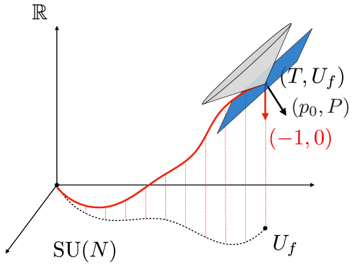
Figure 1: The augmented system $\mathcal{M}:=\mathbb{R}\times\mathrm{SU}(N)$ and the trajectory of the optimal control. The horizontal plane depicts the space $\mathrm{SU}(N)$ and the vertical axis is the extra dimension of time cost. The black dashed curve is a trajectory in the original quantum control system and the red bold curve represents the corresponding trajectory in the augmented system (31). The gray cone is the tent $\tilde{\mathcal{R}}_{(T,U(T))}$. The blue plane is the hyperplane that divides the tangent space at $(T,U(T))$ into a half-space containing the tent and that containing the vector $(-1,0)$. The vector $(p_{0},P)$ is normal to the hyperplane.

4.3 Derivation

We provide a derivation of the statement of MP-QB in Sec. 4.1. Although it is an adaptation of Pontryagin’s MP (e.g. [37]), especially that for control systems on a Lie group (e.g. [39]), to the problem of time-optimal quantum control, it may clarify some subtle points of MP-QB including the difference from the conventional QB. The derivation also reveals the origin of $F(t)$.

Consider an augmented system $\mathcal{M}:=\mathbb{R}\times\mathrm{SU}(N)$ (see Fig. 1). A trajectory ${\left(t,U(t)\right)}$ in $\mathcal{M}$ represents an evolution of a unitary operator $U(t)$ and the time cost $t$ for each $U(t)$ in that evolution.

For a given protocol $H(t)$, the trajectory in $\mathcal{M}$ is determined by the differential equation

$$\dot{t} =1,\quad\dot{U}(t) =-iH(t)U(t).$$ (31)

The reachability set $\mathcal{R}$ in the augmented system is defined by

$$\mathcal{R} :=\bigcup_{t\in[0,\infty]}\mathcal{R}_{t},\quad\mathcal{R}_{t} :={\left\{(t,U(t))|H(t)\in\mathcal{A}\right\}},$$ (32)

where $\mathcal{R}_{t}$ represents the set of all reachable points $U(t)$ at time $t$ and $U(t)$ is generated from the Schrödinger equation (1) with the initial condition $U(0)=1$.

Let the final time $T$ and the protocol $H(t)$ be optimal for given $(U_{f},\mathcal{A})$, so that $U(T)=U_{f}$. Then, the reachability and the optimality imply that the terminal point $(T,U(T))$ of the trajectory $(t,U(t))$ lies at the boundary of $\mathcal{R}$.

We would like to discuss the changes of the point $(T,U(T))$ caused by the changes of the protocol $H(t)$ and the final time $T$. For the former, we employ the needle variation, which is the variation of $H(t)$ on infinitesimal intervals but allows finite changes of $H(t)$ there. This is particularly useful when the optimal protocols may have finite jumps, or when the change of $H(t)\in\mathcal{A}$ is allowed only on one side, i.e., when $\delta H(t)$ is allowed but $-\delta H(t)$ is not. A simple needle variation $M(\tau;\delta\tau;K):H(t)\mapsto H^{\prime}(t)$ at $t=\tau\in(0,T)$ where $H(t)$ is continuous is defined by

$$H^{\prime}(t)=\left\{\begin{array}[]{ll}K,&\tau-\delta\tau<t\leqslant\tau,\\ H(t),&0\leqslant t\leqslant\tau-\delta\tau\mbox{ and }\tau<t\leqslant T,\\ \end{array}\right.$$ (35)

where $\delta\tau\geqslant 0$ is infinitesimal and $K\in\mathcal{A}$. By appropriately defining addition and nonnegative scalar multiplication, which are essentially operations on the time intervals, the needle variations form a space which is closed in those operations, though the “addition” is noncommutative (see A).

The variation $H(t)\mapsto H^{\prime}(t)$ with respect to $T$ is defined as follows. If $\delta T\leqslant 0$, $H^{\prime}(t)$ is simply the restriction of $H(t)$ on the shortened interval, i.e., $H^{\prime}(t)=H(t)$, $0\leqslant t\leqslant T-\delta T$. If $\delta T>0$, $H^{\prime}(t)$ is defined on the extended interval by the value at $t=T$, i.e., $H^{\prime}(t)=H(t)$, $0\leqslant t\leqslant T$ and $H^{\prime}(t)=H(T)$, $t>T$. It can be seen that the combination of the two kinds of variations [of $H(t)$ and $T$] above again form a space which is closed under addition and nonnegative scalar multiplication. Furthermore, though the “addition” is noncommutative, they become commutative in the resulting first-order variation of the final unitary operator $U(T)$ (A). Thus, $\delta{\left[U(T)\right]}$ form a convex cone contained in $T_{(T,U(T))}\mathcal{M}$. This cone is called the tent $\tilde{\mathcal{R}}_{(T,U(T))}$ of ${\mathcal{R}}$ at $(T,U(T))$.

If the tent $\tilde{\mathcal{R}}_{(T,U(T))}$ contains the downward vector $(-1,0)$ in its interior, the protocol ${\left(H(t),F(t)\right)}$ cannot be optimal. This follows from the fact that the deviated points from $(T,U(T))$ by the variations of $H(t)$ and $T$, not only in the first order but to all orders, form a deformed cone in $\mathcal{M}$ that intersects the segment $[0,T)\times{\left\{U_{f}\right\}}$. Thus, if $(H(t),F(t))$ is time optimal, there is a hyperplane that separates the tangent space $T_{(T,U_{f})}\mathcal{M}$ into a closed half-space containing the tent and a closed half-space containing the vector $(-1,0)$. In terms of the normal vector to the hyperplane, there exist a nonzero vector $(p_{0},P)\in T_{(T,U(T))}\mathcal{M}$ such that

$$\left\langle(p_{0},P),\;(-1,0)\right\rangle\geqslant 0\geqslant\left\langle(p_{0},P),\;(\delta T,\,i\delta{\left[U(T)\right]}U(T)^{\dagger})\right\rangle,$$ (36)

where $\delta{\left[U(T)\right]}$ is the first-order variation and the bracket denotes the inner product $\left\langle(q_{0},Q),(r_{0},R)\right\rangle:=q_{0}r_{0}+\tr{\left[QR\right]}$. The first inequality in (36) immediately implies $p_{0}\leqslant 0$.

The first-order variation of $U(T)$ caused by $M(\tau;\delta\tau;K)$ in (35) is

$$\delta U(T)=U(T,\tau){\left(-i\delta\tau{\left[K-H(\tau)\right]}\right)}U(\tau),$$ (37)

where $U(t,\tau)$ is the time evolution operator satisfying the the Schrödinger equation (1) with the initial condition $U(\tau,\tau)=1$. Let us define a Hermitian operator

$$F(t):=U(t,T)PU(T,t).$$ (38)

It is immediately seen that $F$ satisfies the QB equation (27). From (36) and (37), we also have

$$\tr{\left[KF(\tau)\right]}\leqslant\tr{\left[H(\tau)F(\tau)\right]}.$$ (39)

Because $\tau$ is arbitrary, this is nothing but the maximum condition (26).

The first-order variation of $U(T)$ with respect to $T$ is given by

$$\delta{\left[U(T)\right]}=(-i\delta T){H(T)}U(T).$$ (40)

From (36) and (40), and because $\delta T$ can be of both signs, we have

$$\tr{\left[H(T)F(T)\right]}=-p_{0}\geqslant 0.$$ (41)

This is the algebraic condition (29).

5 Drift and inequality constraints

We have discussed MP-QB, a general time-optimal quantum control theory for arbitrary constraints $\mathcal{A}$, where $H(t)\in\mathcal{A}$. For further analysis on the time-optimal control, we discuss the basic structure of $\mathcal{A}$ in this section. We show the conditions under which an inequality constraint can be reduced to an equality one. The use of MP-QB is essential in the following discussion.

5.1 Drift and control Hamiltonians

Let $\mathcal{A}\subset\mathfrak{su}(N)$ be a general constraint (set of available Hamiltonians). Consider the smallest hyperplane that contains $\mathcal{A}$, which we call control hyperplane. Take an arbitrary fixed Hamiltonian $H_{d}\in\mathcal{A}$ and view the hyperplane as a linear subspace $\mathcal{C}$ of $\mathfrak{su}(N)$ whose origin is $H_{d}$. Then, we can write $H(t)\in\mathcal{A}$ as

$$H(t)=H_{d}+H_{c}(t),\quad H_{c}(t)\in\mathcal{A}-H_{d}\;(\subset\mathcal{C}),$$ (42)

where $H_{d}$ is time independent. We call the constraint $H_{c}(t)\in\mathcal{C}$ a subspace constraint and $\mathcal{C}$ the control subspace. We call $H_{d}$ and $H_{c}(t)$ the drift and control Hamiltonians, respectively. Physically, the drift Hamiltonian $H_{d}$ describes the fields intrinsic to the system such as an interaction between the particles with a fixed coupling or a fixed magnetic field. The control Hamiltonian $H_{c}(t)$ describes the fields that we can control, such as a pulse sequence of electromagnetic waves or an adjustable magnetic field.

A subspace constraint can be expressed by equality constraints in the following simple manner. Since the space $\mathfrak{su}(N)$ can be written as

$$\mathfrak{su}(N)=\mathcal{C}\oplus\mathcal{C}^{\perp},$$ (43)

where $\mathcal{C}^{\perp}$ is the orthogonal complement of $\mathcal{C}$ (with respect to the inner product $(1/2)\tr AB$), a subspace constraint $H_{c}(t)\in\mathcal{C}$ is written as

$$\tr{\left[H_{c}(t)\tau_{j}\right]}=0,\quad j=\dim\mathcal{C}+1,\dots,N^{2}-1,$$ (44)

where an orthonormal basis ${\left\{\tau_{j}\right\}}_{j=1}^{N^{2}-1}$ on $\mathfrak{su}(N)$ is chosen so that $\tau_{1},...,\tau_{\dim\mathcal{C}}\in\mathcal{C}$ and $\tau_{\dim\mathcal{C}+1},...,\tau_{N^{2}-1}\in\mathcal{C}^{\perp}$. The total Hamiltonian is written as

$$H(t)=H_{d}+\sum_{j=1}^{l}u^{j}(t)\tau_{j},$$ (45)

with some real variables $u^{j}(t)$.

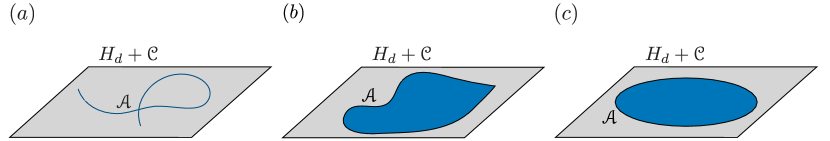
Figure 2: Illustration of (a) general, (b) planar, and (c) typical constraints. Each gray (or bright) plane represents the control hyperplane $H_{d}+\mathcal{C}$ and each blue (or dark) region represents the set $\mathcal{A}$ of all available Hamiltonians.

We shall define a theoretically convenient and practically common class of constraints. We say that a constraint $\mathcal{A}$ is planar if $\mathcal{A}$ is a closed region in $H_{d}+\mathcal{C}$ and $\dim\mathcal{A}=\dim\mathcal{C}$ holds, more precisely, if

$$\mathcal{A}=\mathrm{closure}{\left(\mathrm{interior}(\mathcal{A})\right)}$$ (46)

in the topology of the hyperplane $H_{d}+\mathcal{C}$ (see Fig. 2). We also define a further restricted class. We say that a constraint $\mathcal{A}$ is typical if $\mathcal{A}$ is defined by a subspace constraint $H_{c}(t)\in\mathcal{C}$ and a single inequality

$$\frac{1}{2}\tr{\left[H_{c}(t)^{2}\right]} \leqslant\Omega^{2},$$ (47)

where $\Omega>0$. The constraint (47) is called the finite energy constraint and physically means that the system has a finite energy bandwidth. Thus, $\Omega(>0)$ gives an upper bound of the (Hilbert-Schmidt) norm of the control Hamiltonian. We can write $\mathcal{A}$ of a typical constraint as

$$\mathcal{A} = {\left\{H_{d}+H_{c}\;\middle|\;\tr{\left[H_{c}\tau_{j}\right]}=0,\;j>\dim\mathcal{C},\;\;\frac{1}{2}\tr{\left[H_{c}^{2}\right]}\leqslant\Omega^{2}\right\}},$$ (48)

and the total Hamiltonian as eq. (45) with a constraint $\sum_{j}(u^{j})^{2}\leqslant\Omega$ (see Fig. 2).

5.2 Lollipop-type constraints allow reduction to equality constraints

We divide the general (i.e., not necessarily planar) constraints into two types, whether the drift $H_{d}$ is in the control subspace $\mathcal{C}$ or not. We call the constraint (or $\mathcal{A}$) lollipop type if $H_{d}\in\mathcal{C}$ and lotus leaf type if $H_{d}\not\in\mathcal{C}$ (see Fig. 3). For simplicity and concreteness of the presentation, we first discuss the typical constraints $\mathcal{A}$ and then argue the results apply to the planar constraints as well.

If $\mathcal{A}$ is typical and lollipop type, including the case $H_{d}=0$, the inequality constraint (47) can be reduced to an equality condition,

$$\frac{1}{2}\tr{\left[H_{c}(t)^{2}\right]}=\Omega^{2}.$$ (49)

We give a brief proof. In general, at any instant of time $t$, if we can stretch $H(t)\in\mathcal{A}$ to $aH(t)\in\mathcal{A}$ with $a>1$, we can obtain a faster protocol for the same unitary evolution $U_{f}$. Thus, the time-optimal protocol must not allow such a stretching $a>1$ at any time $t$. As shown in Fig. 3, any $H(t)$ in the interior of $\mathcal{A}$ allow such a stretching. Thus, the time-optimal protocol $H(t)$ must belong to the boundary of $\mathcal{A}$ and satisfy the equality (49) at any time $t$. See also the supplemental material of Ref. [25]. For planar, lollipop-type constraints, the time-optimal control $H(t)$ belongs to the boundary of $\mathcal{A}$ in the hyperplane $H_{d}+\mathcal{C}$. Thus, we can reduce one of the inequalities into the equality, though we may not know which equality is attained. We remark that for non-planar constraints, or $\dim\mathcal{A}<\dim\mathcal{C}$, $H(t)$ always is regarded as being in the boundary of $\mathcal{A}$.

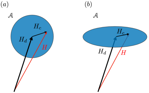
Figure 3: (a) An example of “lollipop-type” constraint for $H$. This is characterized by $H_{d}\in\mathcal{C}$, where $H_{d}$ is the drift Hamiltonian and $\mathcal{C}$ is the control subspace. We can “stretch” the total Hamiltonian $H$ to the boundary of $\mathcal{A}$ while keeping its direction. (b) An example of “lotus leaf-type” constraint, characterized by $H_{d}\not\in\mathcal{C}$. We cannot enlarge the total Hamiltonian $H$ without changing its direction.

5.3 Lotus-leaf-type constraints and a sufficient condition for the reduction

As was defined in the previous subsection, a general constraint $\mathcal{A}$ is called lotus-leaf-type if $H_{d}\notin\mathcal{C}$. For such a constraint, the situation differs from the lollipop-type case.

The reduction of an inequality constraint to an equality constraint by the stretching $aH(t)$ with $a>1$ is not possible in general. We must consider the inequality constraint (47) in detail. This can be seen by a simple example,

$$H(t)=\omega_{0}\sigma^{z}+u(t)\sigma^{x},$$ (50)

for a qubit, where $u(t)$ is a single control variable with $|u(t)|\leqslant\Omega$ [26]. In this case, the control subspace is $\mathcal{C}=\mathbb{R}\sigma^{x}$ and is lotus leaf type. When the target is $U_{f}=e^{-i(\pi/4)\sigma^{z}}$, the time-optimal control is apparently $H(t)=\omega_{0}\sigma^{z}$, hence $u(t)=0$. Thus, the problem is not solved with an equality constraint such as $|u(t)|=\Omega$. It follows that, in general, the inequality constraint is essential for time-optimal control under lotus-leaf-type constraints.

However, we observe by MP-QB that if an additional condition holds, the inequality constraint (47) can be reduced to an equality one (49) for a lotus-leaf-type constraint $\mathcal{A}$ as well. Again, we first discuss the case of typical $\mathcal{A}$ for simplicity and see later that the results hold for planar constraints. Let $\mathcal{A}$ be typical. MP-QB requires the existence of a Hermitian operator $F$ which satisfies the QB equation (27). We assume that $F$ has a nonzero projection onto the subspace $\mathcal{C}$, or $\mathcal{P}_{\mathcal{C}}(F)\neq 0$, where $\mathcal{P}_{\mathcal{C}}$ is an orthogonal projection onto $\mathcal{C}$ as in Fig. 4. Since MP-QB requires the maximization of the Pontryagin Hamiltonian $-1+\tr{\left[H_{d}F\right]}+\tr{\left[H_{c}F\right]}$, the time-optimal Hamiltonian $H$ must maximize the inner product $(1/2)\tr{\left[H_{c}F\right]}$. By the Cauchy-Schwartz inequality, we obtain

$$\tr{\left[H_{c}F\right]}\leqslant\sqrt{\tr{\left[H_{c}^{2}\right]}\tr{\left[\mathcal{P}_{\mathcal{C}}(F)^{2}\right]}}\leqslant\Omega\sqrt{2\tr{\left[\mathcal{P}_{\mathcal{C}}(F)^{2}\right]}}.$$ (51)

This equality is attained if and only if $H_{c}$ is proportional to $\mathcal{P}_{\mathcal{C}}(F)$ and $H_{c}$ has the maximum norm $\Omega$ (see Fig. 4). Therefore, the time-optimal Hamiltonian $H$ must satisfy the equality constraint (49). Note that the “only if” part is guaranteed by the assumption $\mathcal{P}_{\mathcal{C}}(F)\neq 0$.

For a planar constraint $\mathcal{A}$, we can still show that the time-optimal $H$ belongs to the boundary of $\mathcal{A}$, with $\mathcal{A}$ being considered as a subset of the plane $H_{d}+\mathcal{C}$. If $H_{c}$ is in the interior of $\mathcal{A}-H_{d}(\subset\mathcal{C})$, we can take a nonzero variation $\delta H_{c}$ such that $\tr{\left[\delta H_{c}F\right]}>0$ (we still assume $\mathcal{P}_{\mathcal{C}}(F)\neq 0$). Then we can make $\tr{\left[H_{c}F\right]}$ larger by changing $H_{c}$ to $H_{c}+\delta H_{c}$. Note that the assumption $\mathcal{P}_{\mathcal{C}}(F)\neq 0$ guarantees the strict positivity of $\tr{\left[\delta H_{c}F\right]}$. If we say $\mathcal{P}_{\mathcal{C}}(F)\neq 0$ the regularity condition, which is a term introduced in the next section, the result is stated as follows. If the constraint $\mathcal{A}$ is planar, all regular optimal protocols are on the boundary of $\mathcal{A}$.

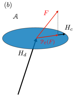
Figure 4: The time-optimal control $H$ in a “lotus-leaf-type” constraint. If we have $\mathcal{P}_{\mathcal{C}}(F)\neq 0$, where $\mathcal{P}_{\mathcal{C}}$ is a projection onto the subspace $\mathcal{C}$, then the inner product $(1/2)\tr{\left[FH_{c}\right]}$ has a maximum when $H_{c}$ is proportional to $\mathcal{P}_{\mathcal{C}}(F)$ with maximal norm.

We have shown by MP-QB that an inequality constraint reduces to an equality one even for the lotus-leaf-type constraint with the help of the assumption $\mathcal{P}_{\mathcal{C}}(F)\neq 0$. Conversely, if this does not hold, the inner product $(1/2)\tr{\left[H_{c}F\right]}$ vanishes for all $H_{c}$ so that the maximization condition (26) gives no information on the optimal Hamiltonian. Such solutions to MP-QB are called singular, which will be discussed in detail in the subsequent section.

6 Singular controls and the generalized Legendre-Clebsch condition

In this section, we shall discuss singular controls. We showed by an example in the previous section that singular controls can be time optimal if $\mathcal{A}$ is lotus leaf type. Inequality constraints cannot be reduced to equality ones for a singular control. We will also see that MP is not powerful enough to determine the optimal protocol from singular ones. Thus, it is desirable to restrict or exclude the possibility of singular protocols to be optimal. We shall give a precise definition of singular protocols in Sec. 6.1 and derive conditions beyond MP that the singular optimal protocols must satisfy in Sec. 6.2. We discuss the physical meaning of singular controls in Sec. 6.3. As before, the problem and the formulation are the same as in Sec. 2 and Sec. 4.1.

6.1 Singular controls

Let $\mathcal{A}$ be a general constraint. We say that a quantum control protocol ${\left(H(t),F(t)\right)}$ is singular at time $t$ if the maximum condition (26) is trivially satisfied for any $H(t)\in\mathcal{A}$, namely, $\tr{\left[KF(t)\right]}=$ constant for all $K\in\mathcal{A}$. In terms of $\mathcal{C}$ and $H_{d}$ in Sec. 5.1, which are determined by $\mathcal{A}$, the singularity condition is equivalent to

$$\tr{\left[\mathcal{C}F(t)\right]} =0,$$ (52)

or $F(t)\perp\mathcal{C}$ (Fig. 4). We call a control ${\left(H(t),F(t)\right)}$ regular at $t$ if it is not singular. If the optimal control $(H(t),F(t))$ is singular in a certain finite time interval containing $t$, the time derivatives of any order of eq. (52) must hold at $t$, that is,

$$\frac{\mathrm{d}^{n}}{\mathrm{d}t^{n}}\tr{\left[\mathcal{C}F(t)\right]}=0,$$ (53)

for $n=1,2,\dots$. For $n=1$, we have

$$\tr{\left[{\left[\mathcal{C},H_{d}\right]}F(t)\right]}=0.$$ (54)

It follows from the algebraic condition (29) of MP-QB and the singularity condition (52) that any optimal singular control ${\left(H(t),F(t)\right)}$ satisfies

$$\tr{\left[H_{d}F(t)\right]} =1.$$ (55)

This in particular implies that if the constraint $\mathcal{A}$ (which is not necessarily planar) is lollipop type, time-optimal singular controls do not exist. This is so because $H_{d}\not\in\mathcal{C}$ is necessary for satisfying eqs. (52) and (54) at the same time.

When singular controls exist, there are two difficulties in finding the time-optimal control. First, MP-QB admits any protocol which is a sequence of regular and singular controls as candidates of the optimal one, so that we do not know in advance how to determine the number and sequence of them. Second, we cannot identify the optimal singular control by MP-QB in general. This is because $H_{\mathrm{{MP}}}$ no longer depends on the control Hamiltonian $H_{c}(t)$ for singular controls and we cannot obtain any information from the maximum condition (26). For the latter problem, however, we will find an additional condition for singular controls to be optimal in Sec. 6.2.

We shall make some comments here on the definition of singular controls. A common definition of a singular control is as follows. Let $\bm{u}\in\mathcal{U}$ be a vector of control variables describing the available Hamiltonian $H\in\mathcal{A}$. Then a control protocol is called singular if there exists a variation of control variables $\delta\bm{u}$, by which the variation of the Pontryagin Hamiltonian $\delta H_{\mathrm{{MP}}}$ vanishes up to the second order (e.g. [30]). In this paper, the control protocol is called singular if the Pontryagin Hamiltonian is constant on $\mathcal{A}$. This definition of singularity is narrowed from the common one in the following two points. First, our definition requires the variation vanishes to all orders. Second, the variation $\delta H_{\mathrm{{MP}}}$ of the Pontryagin Hamiltonian must vanish for $\delta\bm{u}$ in all directions. In particular, we call a protocol regular in the case that some of the control variables are determined by the maximum condition and some are not. Note that, in such cases, we can redefine $\mathcal{A}$ as the subset of the original $\mathcal{A}$ that maximizes $H_{\mathrm{{MP}}}$ and regard the controls as singular ones [30].

6.2 Generalized Legendre-Clebsch condition

We shall derive an additional necessary condition for a singular control to be optimal, which is one of the main results of this paper. The condition can exclude some of the singular protocols from candidates of the optimal ones and is useful in determining the optimal protocol.

Let $H(t)$ be parametrized by control variables $u^{j}(t)$, $1\leqslant j\leqslant l$, in a certain subset $\mathcal{U}\subset\mathbb{R}^{l}$, where we have used up all equality constraints so that all $u^{j}$ are independent. In the following, we assume that the control variables $u^{j}$ are in the interior of $\mathcal{U}$ so that we can take an arbitrary infinitesimal variation of the control variables $u^{j}(t)\rightarrow u^{j}(t)+\delta u^{j}(t)$ at time $t$. Even if the control variables $u^{j}$ are on the boundary of $\mathcal{U}$, we still can regard $u^{j}$ to be in the interior of the boundary of $\mathcal{U}$ by defining new control variables $u^{\prime j}$ with reduced dimensionality, thanks to the implicit function theorem. We can then apply the same arguments below by replacing $u^{j}(t)$ with $u^{\prime j}(t)$ and redefining $l$ as the dimension of $u^{\prime j}$. We will demonstrate the calculations of such a case in Sec. 7 (and in E).

Let us introduce the generalized Legendre-Clebsch (GLC) condition [30]. The GLC condition comes from positive semidefiniteness of the second-order variation of the cost functional $T$ and is useful in determining the singular optimal protocols, where MP becomes trivial. We define an $l\times l$ matrix $Q^{(m)}$, $m=0,1,2\dots$, whose $(i,j)$ element is given by

$$Q^{(m)}_{ij}:=\frac{\partial}{\partial u^{i}}{\left[{\left(\frac{\mathrm{d}}{\mathrm{d}t}\right)}^{m}{\left(\frac{\partial}{\partial u^{j}}H_{\mathrm{{MP}}}{\left(H(t),F(t)\right)}\right)}\right]}.$$ (56)

We denote by $M$ the smallest value of $m$ for which $Q^{(m)}$ has at least one nonzero element. Any optimal control must satisfy the following two conditions:

1. The integer $M$ must be even.

2. If $M=2k$, then $(-1)^{k}Q^{(2k)}$ must be negative semidefinite.

When $M=0$, these yield $Q^{(0)}_{ij}\leqslant 0$ which is implied by MP. When the protocol is singular, $Q^{(0)}_{ij}=0$ and $M>0$ follow. It can also be shown that the matrix $Q^{(m)}$ is symmetric if $m$ is even and anti-symmetric if $m$ is odd. We remark that the GLC condition does not depend on individual representations; although the matrix $Q^{(m)}$ does, the conditions $Q^{(M)}=0$, $Q^{(M)}\geqslant 0$, and $Q^{(M)}\leqslant 0$ do not. See B for a proof.

We shall go back to time-optimal quantum control. We provide the expressions of $Q^{(m)}_{ij}$ for singular protocols so that we can examine the GLC condition in a step-by-step manner. A derivation is given in C. The singularity condition implies $Q^{(0)}_{ij}={\left(\partial^{2}/\partial u^{i}\partial u^{j}\right)}\tr{\left[HF\right]}=0$. Assume that $Q^{(k)}=0$ hold for $k=0,1,\dots,m-1$. Then, $Q^{(m)}_{ij}$ is given by

$$Q^{(m)}_{ij} =-i\tr{\left[{\left[h_{i},F\right]}R^{(m-1)}_{j}\right]},$$ (57)

where $h_{i}:=\partial H/\partial u^{i}$ and $R^{(m)}_{j}$ is obtained by the following recurrence relation,

$$R^{(m)}_{j}=\frac{\mathrm{d}}{\mathrm{d}t}R^{(m-1)}_{j}-i[R^{(m-1)}_{j},H],\quad R^{(0)}_{j}=h_{j}.$$ (58)

In fact, $R^{(m)}_{j}$ is a quantity defined through $H_{\mathrm{{MP}}}$ as $R^{(m)}_{j}:=\frac{\partial}{\partial F}{\left(\frac{\mathrm{d}}{\mathrm{d}t}\right)}^{m}\frac{\partial}{\partial u^{j}}H_{\mathrm{{MP}}}$. We can perform the GLC test in the time-optimal quantum control problem as follows:

1. Let $m=0$. We have $Q^{(m)}=0$.

2. Increase $m$ by one and calculate $Q^{(m)}$ by eqs. (57) and (58).

3. If $Q^{(m)}$ is identically zero, with the help of the previously obtained conditions, go to (1).

4. If $m$ is odd, impose a condition $Q^{(m)}=0$ and go to (1).

5. Impose a condition $(-1)^{k}Q^{(2k)}\leqslant 0$ and halt.

In the special case of planar constraint $\mathcal{A}$, the Hamiltonian $H(t)$ can be written by independent control variables ${\left\{u^{j}\right\}}\in\mathcal{U}$ as

$$H(t)=H_{d}+H_{c}(t)=H_{d}+\sum_{j=1}^{l}u^{j}(t)h_{j}.$$ (59)

Then, $h_{j}$ appearing in eqs. (57) and (58) become fixed, time-independent operators in $\mathfrak{su}(N)$, which span the control subspace $\mathcal{C}$. We give concrete expressions for the first few $Q^{(m)}_{ij}$ in this case:

$$Q_{ij}^{(1)} =-i\tr{\left[{\left[h_{j},h_{i}\right]}F\right]},$$

$$Q_{ij}^{(2)} =\tr{\left[{\left[{\left[H,h_{j}\right]},h_{i}\right]}F\right]},$$

$$Q_{ij}^{(3)} =i\tr{\left[{\left[{\left[H,{\left[H,h_{j}\right]}\right]},h_{i}\right]}F\right]}+\tr{\left[{\left[{\left[\frac{\mathrm{d}H}{\mathrm{d}t},h_{j}\right]},h_{i}\right]}F\right]}.$$ (60)

For example, the GLC condition for $m=1$ reads $\tr{\left[{\left[h_{i},h_{j}\right]}F\right]}=0$ for $1\leqslant i,j\leqslant l$. This is equivalent to

$$\tr{\left[[\mathcal{C},\mathcal{C}]F\right]}=0.$$ (61)

From this condition, we observe that time-optimal singular controls exist only when $H_{d}\not\in[\mathcal{C},\mathcal{C}]$. For otherwise, eq. (61) would imply $\tr{\left[H_{d}F\right]}=0$, which would contradict eq. (55).

6.3 Physical meaning of singular controls

In considering the physical meaning of the singular controls, we naively expect that the regular control takes advantage of the control Hamiltonian $H_{c}$ and the singular control takes advantage of the drift Hamiltonian $H_{d}$. This naive expectation is supported by the following facts. (i) For typical $\mathcal{A}$, the regular optimal controls necessarily attain the maximal norm of the control Hamiltonian; for planar $\mathcal{A}$, the regular optimal controls must be on the boundary of $\mathcal{A}$. (ii) For planar $\mathcal{A}$, optimal singular controls exist only when the drift Hamiltonian $H_{d}$ satisfies the conditions $H_{d}\not\in\mathcal{C}$ and $H_{d}\not\in[\mathcal{C},\mathcal{C}]$. The latter two conditions imply that $H_{c}(t)$ cannot help generate unitary operator $e^{-i\alpha H_{d}}$ up to the second-order of infinitesimal time interval $\delta t$. This follows from the Baker-Campbell-Hausdorff formula. For example, we assume $H(t)=H_{d}+K_{1}$ for $t\in[0,\delta t]$ and $H(t)=H_{d}+K_{2}$ for $t\in[\delta t,2\delta t]$, where $K_{1},K_{2}\in\mathcal{C}$ and $H_{d}\not\in\mathcal{C},[\mathcal{C},\mathcal{C}]$. Then, we have the resulting unitary operator $U(2\delta t)$ as

$$U(2\delta t)=e^{-i\delta t(H_{d}+K_{2})}e^{-i\delta t(H_{d}+K_{1})}$$

$$=\exp{\left[-2i\delta tH_{d}+\delta t(K_{1}+K_{2})+\frac{\delta t^{2}}{2}{\left[H_{d}+K_{2},H_{d}+K_{1}\right]}+\mathcal{O}(\delta t^{3})\right]},$$ (62)

where $H_{d}\not\in\mathcal{C},[\mathcal{C},\mathcal{C}]$ ensures that the second and third terms in the argument of the exponential cannot produce a term proportional to $H_{d}$.

7 Examples

In this section, we shall discuss three examples of systems where singular controls are present. We will see how the methods and the results in the previous sections work. The first two examples are revisits to previously analyzed, simple two-dimensional systems. The first example allows an optimal singular control. The second allows singular controls but they turn out non-optimal thanks to the GLC condition. The third example is a three-dimensional system where singular controls have not been analyzed in detail. We will see that the GLC condition excludes some singular controls from being optimal but the others survive. However, we will observe that consideration of only a single singular control is enough.

7.1 Example 1: Landau-Zener model

First, let us seek the time-optimal controls in the Landau-Zener model,

$$H(t)=\omega_{0}\sigma^{z}+u(t)\sigma^{x},$$ (63)

where $\omega_{0}>0$ is a fixed parameter and $u(t)$ is a control variable satisfying $|u(t)|\leqslant\Omega$, as in Ref. [26]. We have the drift $H_{d}=\omega_{0}\sigma^{z}$ and the control subspace $\mathcal{C}=\mathrm{span}\,{\left\{\sigma^{x}\right\}}$. The set $\mathcal{A}$ of available Hamiltonians is typical and lotus leaf type. From eq. (52), a control is singular if

$$\tr[\sigma^{x}F] =0.$$ (64)

The time derivatives of this conditions are

$$\frac{\mathrm{d}}{\mathrm{d}t}\tr[\sigma^{x}F] =-i\tr[\sigma^{x}[H,F]]=-2\omega_{0}\tr[\sigma^{y}F]=0,$$ (65)

$$\frac{\mathrm{d}^{2}}{\mathrm{d}t^{2}}\tr[\sigma^{x}F] =2i\omega_{0}\tr[\sigma^{y}[H,F]]=4\omega_{0}u(t)\tr[\sigma^{z}F]=0.$$ (66)

If the singular control is time optimal, we have from (55) that

$$\tr{\left[H_{d}F\right]}=\omega_{0}\tr[\sigma^{z}F] =1.$$ (67)

Eqs. (66) and (67) imply $u(t)=0$. This is the only singular control that is potentially time optimal. The GLC condition does not exclude this protocol, which can be verified through eqs. (60). Ref. [26] actually provides a case, though it is for the evolution of quantum states, that the “bang-off-bang” control is optimal, where the “bang” control $u(t)=\pm\Omega$ is regular and the “off” control $u(t)=0$ is singular.

7.2 Example 2: one-qubit system

Next, we discuss the one-qubit example raised at the end of Sec. 2. The Hamiltonian reads

$$H(t)=\omega_{0}\sigma^{z}+u^{x}(t)\sigma^{x}+u^{y}(t)\sigma^{y},$$ (68)

where $\omega_{0}>0$ is a fixed parameter and $u^{x}(t)$ and $u^{y}(t)$ are control variables satisfying $(u^{x})^{2}+(u^{y})^{2}\leqslant\Omega$. We have the drift $H_{d}=\omega_{0}\sigma^{z}$ and the control subspace $\mathcal{C}=\mathrm{span}\,{\left\{\sigma^{x},\sigma^{y}\right\}}$. The constraint $\mathcal{A}$ is typical and lotus leaf type.

The singularity condition for $(H(t),F(t))$ is given by $\tr[\mathcal{C}F]=0$, or

$$\tr{\left[\sigma^{x}F\right]}=\tr{\left[\sigma^{y}F\right]}=0.$$ (69)

We can show that the singular control has $u^{x}=u^{y}=0$ in a way similar to the previous example. If this singular protocol is time optimal, it is necessary that

$$\tr{\left[\sigma^{z}F\right]}=1.$$ (70)

Here, we show by the GLC condition that the singular controls cannot be optimal. From eq. (60), where $h_{1}=\sigma^{x}$ and $h_{2}=\sigma^{y}$, we have the $(1,2)$-component of the matrix $Q^{(1)}$,

$$Q^{(1)}_{12}=-i\tr{\left[{\left[\sigma^{x},\sigma^{y}\right]}F\right]}=2\tr{\left[\sigma^{z}F\right]}.$$ (71)

The GLC condition implies that this must vanish. This contradicts eq. (70). Therefore, the singular control $u^{x}=u^{y}=0$ is not time optimal. Although this statement has already been shown in Ref. [23], the proof has become easier thanks to the GLC condition.

7.3 Example 3: symmetric two-qubit system

Our final example is a quantum control in a three-dimensional Hilbert space. We adopt a representation by two spins. Consider a Hamiltonian

$$H_{2}(t)=\omega_{0}\sigma^{x}_{1}\sigma^{x}_{2}+J(t)\sigma^{z}_{1}\sigma^{z}_{2}+\sum_{i=1}^{3}\frac{b^{i}(t)}{2}{\left(\sigma^{i}_{1}+\sigma^{i}_{2}\right)},$$ (72)

where $\omega_{0}>0$ is a fixed parameter and $(J,b^{1},b^{2},b^{3})\in\mathbb{R}^{4}$ are control variables in the region $J^{2}+(b^{1})^{2}+(b^{2})^{2}+(b^{3})^{2}\leqslant\Omega^{2}$ denoted by $\mathcal{U}\subset\mathbb{R}^{4}$. We assume $\omega_{0}<\Omega$.

The Hamiltonian is symmetric under the exchange of the spins. Thus, the symmetric subspace $\mathcal{H}_{\mathrm{sym}}$ of the total Hilbert space $\mathcal{H}$, or the space of triplet states, is invariant under the time evolution by $U(t)$. We hereafter restrict our attention on $\mathcal{H}_{\mathrm{sym}}$. This is a control problem on $\mathrm{SU}(3)$. On $\mathcal{H}_{\mathrm{sym}}$, we can rewrite the Hamiltonian $H_{2}(t)$ as

$$H(t)=\omega_{0}\tilde{\Sigma}^{x}+J(t)\tilde{\Sigma}^{z}+\sum_{i}b^{i}(t)S^{i},$$ (73)

where $\Sigma^{x},\Sigma^{z},S^{1},S^{2}$, and $S^{3}$ are the restrictions on $\mathcal{H}_{\mathrm{sym}}$ of $\sigma^{x}_{1}\sigma^{x}_{2},\sigma^{z}_{1}\sigma^{z}_{2},(\sigma^{x}_{1}+\sigma^{x}_{2})/2,(\sigma^{y}_{1}+\sigma^{y}_{2})/2$, and $(\sigma^{z}_{1}+\sigma^{z}_{2})/2$, respectively, and the tilde denotes the traceless part on $\mathcal{H}_{\mathrm{sym}}$. Concrete expressions for them are given in D.

For the Hamiltonian (73), we have

$$H_{d}=\omega_{0}\tilde{\Sigma}^{x},\quad H_{c}(t)=J(t)\tilde{\Sigma}^{z}+\sum_{i}b^{i}(t)S^{i},$$ (74)

$$\mathcal{C}=\mathrm{span}\,{\{\tilde{\Sigma}^{z},S^{1},S^{2},S^{3}\}}=\mathrm{span}\,{\{\lambda_{1}+\lambda_{6},\,\lambda_{2}+\lambda_{7},\,\lambda_{3},\,\lambda_{8}\}},$$ (75)

where ${\left\{\lambda_{i}\right\}}_{i=1}^{8}$ are the Gell-Mann matrices (D). The constraint $\mathcal{A}$ is planar and lotus leaf type. Note that the constraint is typical as a two-qubit problem (on $\mathcal{H}$) but is not so as a one-qutrit problem (on $\mathcal{H}_{\mathrm{sym}}$).

Let us identify the singular controls $(H(t),F(t))$. We expand $F$ by the Gell-Mann matrices, $F=\sum_{i=1}^{8}f^{i}\lambda_{i}$. The singularity condition (52) and its derivative (54) imply that

$$f^{1}+f^{6}=f^{2}+f^{7}=f^{3}=f^{8}=f^{5} =0.$$ (76)

Under these relations, the algebraic condition (29) [or (52)] leads to

$$f^{4}\neq 0.$$ (77)

In the following, we perform the GLC test. We discuss here the case that $(J,b^{1},b^{2},b^{3})$ is in the interior of $\mathcal{U}$, while we show non-optimality of the singular controls on the boundary of $\mathcal{U}$ in E. We calculate the matrix $Q^{(1)}$ by eqs. (60) with $h_{j}=S^{j}$ for $j=1,2,3$ and $h_{4}=\tilde{\Sigma}^{z}$. The only nontrivial components are

$$Q^{(1)}_{41} =-Q^{(1)}_{14}=i4\sqrt{2}f^{2},\quad Q^{(1)}_{42} =-Q^{(1)}_{24}=-i4\sqrt{2}f^{1}.$$ (78)

The GLC condition $Q^{(1)}=0$ requires $f^{1}=f^{2}=0$. It follows that $f^{i}=0$ except $i=4$. Then, from the conditions $\mathrm{d}f^{i}/\mathrm{d}t=-i\tr{\left[\lambda_{i}[H,F]\right]}=0$ for $i\neq 4$, we have

$$b^{i}=0,\quad i=1,2,3.$$ (79)

Therefore, all variables other than $f^{4}$ and $J$ are zero by the GLC condition for $m=1$. Next, we calculate $Q^{(2)}$ to obtain

$$Q^{(2)}=4{\small\left(\begin{array}[]{cccc}Jf^{4}&0&0&0\\ 0&(\omega_{0}-J)f^{4}&0&0\\ 0&0&2f^{4}\omega_{0}&0\\ 0&0&0&0\end{array}\right){}}.$$ (84)

From the GLC condition, $Q^{(2)}$ must be positive semidefinite, which implies

$$0\leqslant f^{4},\quad 0\leqslant J\leqslant\omega_{0}.$$ (85)

This is the condition that singular optimal controls must satisfy. As a result, the singular time-optimal Hamiltonian has the form

$$H(t)=\omega_{0}\tilde{\Sigma}^{x}+J(t)\tilde{\Sigma}^{z},$$ (86)

where $0\leqslant J(t)\leqslant\omega_{0}$.

However, a further observation shows that we can restrict the time-optimal singular controls to

$$H(t)=H_{d}=\omega_{0}\tilde{\Sigma}^{x}$$ (87)

only, because we can replace any optimal singular protocol (86) with a regular protocol followed by the protocol (87) without changing the time duration. Assume that a time-optimal protocol $H(t)$ in the interval $[t_{1},t_{2}]$ is given by eq. (86). Then, the unitary operator in $[t_{1},t_{2}]$ is given by

$$U_{\mathrm{sing}}(t_{2},t_{1})=e^{-i\omega_{0}(t_{2}-t_{1})\tilde{\Sigma}^{x}}e^{-i{\left(\int_{t_{1}}^{t_{2}}dt\;J(t)\right)}\tilde{\Sigma}^{z}},$$ (88)

because $\tilde{\Sigma}^{z}$ and $\tilde{\Sigma}^{x}$ commute. Since $J<\Omega$, there exists $t_{3}\in[t_{1},t_{2}]$ such that

$$\int_{t_{1}}^{t_{2}}dt\;J(t)=(t_{3}-t_{1})\Omega.$$ (89)

We can realize the unitary operator (88) by setting $J(t)=\Omega$ on $[t_{1},t_{3}]$ and $J(t)=0$ on $[t_{3},t_{2}]$. Since the control $J=\Omega$ cannot be singular optimal [as was seen in (85)], it is regular. Therefore, we can deform any time-optimal singular control to a regular control plus the singular control given by eq. (87). Thus, we can restrict ourselves to seek a sequence consisting of regular solutions of MP-QB and a singular control $H(t)=H_{d}$. In fact, if the target unitary operator $U_{f}$ takes the form

$$U_{f}=e^{-i\alpha\tilde{\Sigma}^{x}},$$ (90)

then the singular control with $H_{c}=0$ may be optimal and the time cost is $\alpha/\omega_{0}$.

8 Conclusion and discussions

We have discussed the problem of finding the time-optimal control on quantum systems. The problem is specified by a pair $(U_{f},\mathcal{A})$, where $\mathcal{A}\subset\mathfrak{su}(N)$ is the set of available Hamiltonians representing the theoretical or experimental constraints on the system and $U_{f}\in\mathrm{SU}(N)$ is the target unitary operation. Our task is to find the Hamiltonian $H(t)\in\mathcal{A}$ which realizes $U_{f}$ in the least time. Although there has been a formulation by variational principle called quantum brachistochrone (QB) [12, 13], it has a drawback that it is applicable only when $\mathcal{A}$ is expressed by a set of equalities. To treat inequality constraints as well, we have extended QB by Pontryagin’s maximum principle which can be viewed as a modern variational calculus. The new formulation, which we called MP-QB in this paper, requires the maximization of a quantity known as the Pontryagin Hamiltonian with respect to the control Hamiltonians at each instant of time. The solutions to MP-QB fall into either of the two types, regular and singular controls. The singular controls are those for which the Pontryagin Hamiltonian does not depend on the control Hamiltonian and therefore we cannot determine the optimal control protocol from MP-QB. To overcome this issue, we have introduced an additional necessary condition for the optimum, that is, the generalized Legendre-Clebsch (GLC) condition. We have rewritten the condition as a form suitable for quantum time-optimal control. This enable us to restrict the form of the optimal singular Hamiltonians. This has been demonstrated in the examples. To summarize, we have constructed a general theory and a procedure to find the time-optimal control in quantum systems which can take care of inequality constraints and singular protocols.

Taking advantage of generality of MP-QB, we have also discussed the relation among the drift field, the reduction of inequality constraints, and the singular controls. To do so, we have classified the general constraint $\mathcal{A}$ into two types, the lollipop type and the lotus leaf type, depending on the drift $H_{d}$ belongs to the control subspace $\mathcal{C}$ or not. We have also introduced a useful class of constraints, called planar constraints, which covers most of commonly encountered situations. We have shown the following.

1. If the constraint $\mathcal{A}$ is lollipop type, there do not exist time-optimal singular controls (Sec. 6.1).

2. If the constraint $\mathcal{A}$ is planar, all regular optimal controls lie on the boundary of $\mathcal{A}$ (in the control hyperplane $H_{d}+\mathcal{C}$), i.e., attain an equality among the inequality constraints (Sec. 5.2 and Sec. 5.3).

From (i) and (ii), if $\mathcal{A}$ is planar and the lollipop type, all optimal controls are regular and attain an equality. On the other hand, if $\mathcal{A}$ is lotus leaf type, such reduction depends on the situation (see Sec.7).

Therefore, an efficient procedure to find the time-optimal control protocol for the system with inequality constraints is as follows. First, check whether the system constraint is lollipop type or lotus leaf type. If the constraint is lollipop type, the optimal control is regular. Otherwise, the optimal control possibly consists of regular and singular controls. The regular optimal controls attain an equality and one can identify the time-optimal protocol by the QB equation as in the previous studies [13]. Because the singular optimal controls are not identified by the maximum principle, one must carry out the GLC test. To summarize, the time-optimal control is a solution of the QB equation (regular control) for lollipop-type constraints and is a certain sequence consisting of solutions to QB equation (regular controls) and singular controls that satisfy the GLC condition for lotus-leaf-type constraints.

By MP-QB and the GLC condition, we also have provided an intuitive understanding that the regular control takes advantage of the control Hamiltonian whereas the singular control takes advantage of the drift Hamiltonian. This is best seen in the systems with typical constraints: the regular controls must have the maximal norm of the control Hamiltonian; singular controls exist only when the drift field $H_{d}$ is not in $\mathcal{C}$ or $[\mathcal{C},\mathcal{C}]$ so that the control Hamiltonian $H_{c}\in\mathcal{C}$ cannot be of much help to $H_{d}$. The examples in the last section had such singular controls. Although a similar argument is possible for planar constraints, whether such an interpretation is possible in general is open.

Appendix A Construction of tent and its convexity

In this appendix, we shall construct the tent $\tilde{\mathcal{R}}_{(T,U(T))}$ of $\mathcal{R}$ at $(T,U(T))\in\mathcal{M}$ mentioned in Sec. 4.3 and prove its convexity.

We first show that the needle variations form a space which is closed under addition and non-negative scalar multiplication. These operations are intuitively the corresponding operations on intervals of the variations. A simple needle variation $M(\tau;\delta\tau;K)$ is defined in eq. (35). The sum $M(\tau_{1};\delta\tau_{1};K_{1})+M(\tau_{2};\delta\tau_{2};K_{2})$ of needle variations is defined simply by the composition of these operations if $\tau_{1}\neq\tau_{2}$. If $\tau_{1}=\tau_{2}=:\tau$, the sum is given by arranging them “side by side,” namely, the resulting $H^{\prime}(t)$ is given by

$$H^{\prime}(t)=\left\{\begin{array}[]{ll}K_{1},&\tau-\delta\tau_{1}-\tau_{2}<t\leqslant\tau-\delta\tau_{2},\\ K_{2},&\tau-\delta\tau_{2}<t\leqslant\tau,\\ H(t),&\mbox{otherwise}.\end{array}\right.$$ (94)

The sum of the sums of simple needle variations, etc., are defined in a similar manner. The space of needle variations thus constructed is closed under “addition,” which is not commutative. A non-negative scalar multiplication is defined by scalar multiplications on all the intervals. For example, we have $\lambda{\left(M(\tau_{1};\delta\tau_{1};K_{1})+M(\tau_{2};\delta\tau_{2};K_{2})\right)}=M(\tau_{1};\lambda\delta\tau_{1};K_{1})+M(\tau_{2};\lambda d\tau_{2};K_{2})$. Under these operations, the space of needle variations is closed. Including variations of $\delta T$ defined in Sec. 4.3, The space of variations is still closed under addition and non-negative scalar multiplication.

Second, although the “addition” of needle variations of $H(t)$ are non-commutative, that of the resulting variations of $U(T)$ are commutative. This can be seen by the fact that the variation of $U(T)$ caused by $M(\tau;\delta\tau_{1};K_{1})+M(\tau;\delta\tau_{2};K_{2})$ is

$$\delta U(T)=-iU(T,\tau){\left[\delta\tau_{1}(K_{1}-H(\tau))+\delta\tau_{2}(K_{2}-H(\tau))\right]}U(\tau),$$ (95)

which is commutative. Thus, the first-order variations $\delta{\left[U(T)\right]}$ with respect to the needle variations and the final time variation form a convex-linear space. This convex cone is the tent $\tilde{R}_{(T,U(T))}$.

Appendix B Invariance of the GLC condition under coordinate transformation

The matrix $Q^{(m)}$ depends on parametrizations of the same Hamiltonians. We shall show that the conditions $Q^{(M)}=0$, $Q^{(M)}\geqslant 0$, or $Q^{(M)}\leqslant 0$ are nevertheless equivalent in any parametrization.

Let $\bm{u}={\left\{u^{j}(t)\right\}}$ and $\bm{v}={\left\{v^{j}(t)\right\}}$ be parametrizations of the same Hamiltonian $H(t)$. We have

$$\frac{\partial}{\partial u^{i}} =\sum_{j=1}^{l}\frac{\partial v^{j}}{\partial u^{i}}\frac{\partial}{\partial v^{j}},$$ (96)

where the Jacobi matrix $\partial v^{j}/\partial u^{i}$ is invertible.

First, we will derive the relation between $Q^{(M)}(\bm{u})$ and $Q^{(M^{\prime})}(\bm{v})$, where we define $M,M^{\prime}$ are the smallest value of $m,m^{\prime}$ for which $Q^{(M)}(\bm{u})$, $Q^{(M^{\prime})}(\bm{v})$ have at least one nonzero element respectively. We can assume $M\leqslant M^{\prime}$ without loss of generality. Direct application of (96) to (56) leads to

$$Q^{(M)}_{ij}(\bm{u}) =\sum_{k,l=1}^{l}\frac{\partial v^{k}}{\partial u^{i}}\frac{\partial}{\partial v^{k}}{\left[{\left(\frac{\mathrm{d}}{\mathrm{d}t}\right)}^{M}{\left(\frac{\partial v^{l}}{\partial u^{j}}\frac{\partial}{\partial v^{l}}H_{\mathrm{{MP}}}\right)}\right]}$$ (99)

$$=\sum_{k,l=1}^{l}\frac{\partial v^{k}}{\partial u^{i}}\frac{\partial v^{l}}{\partial u^{j}}\frac{\partial}{\partial v^{k}}{\left[{\left(\frac{\mathrm{d}}{\mathrm{d}t}\right)}^{M}{\left(\frac{\partial}{\partial v^{l}}H_{\mathrm{{MP}}}\right)}\right]}$$

$$+\sum_{n=1}^{M}\small\left(\begin{array}[]{c}M\\ n\end{array}\right){}\sum_{k,l=1}^{l}\frac{\partial v^{k}}{\partial u^{i}}\frac{\partial}{\partial v^{k}}{\left[{\left(\frac{\mathrm{d}}{\mathrm{d}t}\right)}^{n}{\left(\frac{\partial v^{l}}{\partial u^{j}}\right)}{\left(\frac{\mathrm{d}}{\mathrm{d}t}\right)}^{M-n}{\left(\frac{\partial}{\partial v^{l}}H_{\mathrm{{MP}}}\right)}\right]}.$$

However, the last terms vanish because we have $Q^{(m)}(\bm{v})=0$ for $m<M^{\prime}$ and

$${\left(\frac{\mathrm{d}}{\mathrm{d}t}\right)}^{m}{\left(\frac{\partial}{\partial v^{l}}H_{\mathrm{{MP}}}\right)}=0$$ (100)

from eq. (53). Therefore, we obtain

$$Q^{(M)}_{ij}(\bm{u}) =\frac{\partial v^{k}}{\partial u^{i}}Q^{(M)}_{kl}(\bm{v})\frac{\partial v^{l}}{\partial u^{j}}.$$ (101)

Since the matrix $\partial v^{j}/\partial u^{i}$ is invertible, we have $Q^{(M)}(\bm{u})=0\Leftrightarrow Q^{(M)}(\bm{v})=0$, $Q^{(M)}(\bm{u})\geqslant 0\Leftrightarrow Q^{(M)}(\bm{v})\geqslant 0$, and $Q^{(M)}(\bm{u})\leqslant 0\Leftrightarrow Q^{(M)}(\bm{v})\leqslant 0$.

Appendix C Recurrence relation of the matrix $Q^{(m)}$

We shall demonstrate the calculation of the matrix $Q^{(m)}$ in our formulation in Sec. 6.

First, we obtain the recurrence relation for general $m>0$ as

$$Q^{(m)}_{ij} =\frac{\partial}{\partial u^{i}}{\left[\frac{\mathrm{d}}{\mathrm{d}t}{\left(\frac{\mathrm{d}}{\mathrm{d}t}\right)}^{m-1}\frac{\partial}{\partial u^{j}}H_{\mathrm{{MP}}}\right]}$$ (102)

$$=\frac{\partial}{\partial u^{i}}{\left[\frac{\mathrm{d}u^{k}}{\mathrm{d}t}\frac{\partial}{\partial u^{k}}{\left(\frac{\mathrm{d}}{\mathrm{d}t}\right)}^{m-1}\frac{\partial}{\partial u^{j}}H_{\mathrm{{MP}}}+\tr{\left[\frac{\mathrm{d}F}{\mathrm{d}t}\frac{\partial}{\partial F}{\left(\frac{\mathrm{d}}{\mathrm{d}t}\right)}^{m-1}\frac{\partial}{\partial u^{j}}H_{\mathrm{{MP}}}\right]}\right]}$$

$$=\frac{\mathrm{d}}{\mathrm{d}t}Q^{(m-1)}_{ij}-i\tr{\left[{\left[\frac{\partial H}{\partial u^{i}},F\right]}R^{(m-1)}_{j}\right]},$$

where we define

$$R^{(m)}_{j}:=\frac{\partial}{\partial F}{\left(\frac{\mathrm{d}}{\mathrm{d}t}\right)}^{m}\frac{\partial}{\partial u^{j}}H_{\mathrm{{MP}}}.$$ (103)

For $m=0$, we can calculate

$$R^{(0)}_{j}=\frac{\partial}{\partial F}\tr{\left[\frac{\partial H}{\partial u^{j}}F\right]}=\frac{\partial H}{\partial u^{j}},$$ (104)

and can similarly show

$$R^{(m)}_{j} =\frac{\mathrm{d}u^{k}}{\mathrm{d}t}\frac{\partial}{\partial u^{k}}R^{(m-1)}_{j}+\frac{\partial}{\partial F}\tr{\left[\frac{\mathrm{d}F}{\mathrm{d}t}R^{(m-1)}_{j}\right]}$$ (105)

$$=\frac{\mathrm{d}}{\mathrm{d}t}R^{(m-1)}_{j}-i{\left[R^{(m-1)}_{j},H\right]},$$

for general $m>0$.

If $Q^{(k)}=0$ for $k=1,2,\dots,m-1$ for a certain $m>0$, then eq. (102) becomes

$$Q^{(m)}_{ij}=-i\tr{\left[{\left[\frac{\partial H}{\partial u^{i}},F\right]}R^{(m-1)}_{j}\right]}.$$ (106)

For $m=1$, we have

$$Q^{(1)}_{ij} =-i\tr{\left[{\left[\frac{\partial H}{\partial u^{j}},\frac{\partial H}{\partial u^{i}}\right]}F\right]}.$$ (107)

For $m=2$, we have

$$Q^{(2)}_{ij} =-i\tr{\left[{\left[\frac{\mathrm{d}}{\mathrm{d}t}{\left(\frac{\partial H}{\partial u^{j}}\right)},\frac{\partial H}{\partial u^{i}}\right]}F\right]}-\tr{\left[{\left[\frac{\partial H}{\partial u^{i}},F\right]}{\left[\frac{\partial H}{\partial u^{j}},H\right]}\right]}.$$ (108)

The first term in $Q^{(2)}_{ij}$ above vanishes when $\partial H/\partial u^{j}$ is time independent.

Appendix D Operators appearing in Example 3

We list some operators appearing in Example 3 (Sec. 7.3).

The Gell-Mann matrices are defined as

$$\lambda_{1} ={\small\left(\begin{array}[]{ccc}0&1&0\\ 1&0&0\\ 0&0&0\end{array}\right){}},\quad\lambda_{2}={\small\left(\begin{array}[]{ccc}0&-i&0\\ i&0&0\\ 0&0&0\end{array}\right){}},\quad\lambda_{3}={\small\left(\begin{array}[]{ccc}1&0&0\\ 0&-1&0\\ 0&0&0\end{array}\right){}},$$ (118)

$$\lambda_{4} ={\small\left(\begin{array}[]{ccc}0&0&1\\ 0&0&0\\ 1&0&0\end{array}\right){}},\quad\lambda_{5}={\small\left(\begin{array}[]{ccc}0&0&-i\\ 0&0&0\\ i&0&0\end{array}\right){}},\quad\lambda_{6}={\small\left(\begin{array}[]{ccc}0&0&0\\ 0&0&1\\ 0&1&0\end{array}\right){}},$$ (128)

$$\lambda_{7} ={\small\left(\begin{array}[]{ccc}0&0&0\\ 0&0&-i\\ 0&i&0\end{array}\right){}},\quad\lambda_{8}={\small\frac{1}{\sqrt{3}}\left(\begin{array}[]{ccc}1&0&0\\ 0&1&0\\ 0&0&-2\end{array}\right){}}.$$ (135)

They form the orthonormal basis for $\mathfrak{su}(3)$.

The operators on $\mathcal{H}_{\mathrm{sym}}$ appeared in Sec. 7.3 has the following forms in the basis ${\left\{\ket{\uparrow\uparrow},(\ket{\uparrow\downarrow}+\ket{\downarrow\uparrow})/2,\ket{\downarrow\downarrow}\right\}}$:

$$\Sigma^{x}=\small\left(\begin{array}[]{ccc}0&0&1\\ 0&1&0\\ 1&0&0\end{array}\right){},\quad\Sigma^{z}=\small\left(\begin{array}[]{ccc}1&0&0\\ 0&-1&0\\ 0&0&1\end{array}\right){},\quad S^{1}={\small\frac{1}{\sqrt{2}}\left(\begin{array}[]{ccc}0&1&0\\ 1&0&1\\ 0&1&0\end{array}\right){}},$$ (145)

$$S^{2}={\small\frac{1}{\sqrt{2}}\left(\begin{array}[]{ccc}0&-i&0\\ i&0&-i\\ 0&i&0\end{array}\right){}},\;S^{3}=\small\left(\begin{array}[]{ccc}1&0&0\\ 0&0&0\\ 0&0&-1\end{array}\right){}.$$ (152)

The traceless parts of $\Sigma^{i}$ on $\mathcal{H}_{\mathrm{sym}}$ are given by $\tilde{\Sigma}^{i}=\Sigma^{i}-1/3$ while $S^{i}$ are traceless themselves. By using the Gell-Mann matrices, we have

$$\tilde{\Sigma}^{x} =\lambda_{4}-\frac{1}{2}\lambda_{3}+\frac{1}{2\sqrt{3}}\lambda_{8},\quad\tilde{\Sigma}^{z}=\lambda_{3}-\frac{1}{\sqrt{3}}\lambda_{8},$$

$$S^{x} =\frac{1}{\sqrt{2}}{\left(\lambda_{1}+\lambda_{6}\right)},\quad S^{y}=\frac{1}{\sqrt{2}}{\left(\lambda_{2}+\lambda_{7}\right)},\quad S^{z}=\frac{1}{2}{\left(\lambda_{3}+\sqrt{3}\lambda_{8}\right)}.$$ (153)

Appendix E The GLC condition for boundary singular controls in Example 3

In this appendix, we shall show that boundary singular controls in Example 3 (Sec. 7.3) with

$$J^{2}+(b^{1})^{2}+(b^{2})^{2}+(b^{3})^{2}=\Omega^{2}$$ (154)

are not optimal. We will reduce the number of control variables and apply the GLC condition.

We begin with recalling the conditions that hold in general. The singularity condition (52) and its derivative (54) imply eqs. (76), (77) and the following:

$$b^{1}f^{2}-b^{2}f^{1} =0,$$ (155)

$$Jf^{2} =0,$$ (156)

$$f^{1}(J-\omega_{0}) =0.$$ (157)

The second time derivative implies

$$b^{1}f^{1}+b^{2}f^{2}+\sqrt{2}b^{3}f^{4} =0.$$ (158)

The algebraic condition (29) leads to $f^{4}\neq 0$ [eq. (77)]. These hold for both interior and boundary singular controls.

Let us perform the GLC test. We shall show by contradiction that singular optimal controls must have $b^{i}=0(i=1,2,3)$ and then examine the optimality of such protocols.

First, we assume $b^{3}\neq 0$. We regard the Hamiltonian (73) as a function of $b^{1}$, $b^{2}$ and $J$,

$$H(t)=\omega_{0}\tilde{\Sigma}^{x}+J\tilde{\Sigma}^{z}+\sum_{i=1}^{2}b^{i}(t)S^{i}+b^{3}(b^{1},b^{2},J;t)S^{3},$$ (159)

where $b^{3}(b^{1},b^{2},J;t)=\pm\sqrt{\Omega^{2}-J^{2}-(b^{1})^{2}-(b^{2})^{2}}$. We have

$$h_{i}:=\frac{\partial H}{\partial b^{i}} =S^{i}-\frac{b^{i}}{b^{3}}S^{3}\quad(i=1,2),$$

$$h_{3}:=\frac{\partial H}{\partial J} =\tilde{\Sigma}^{z}-\frac{J}{b^{3}}S^{3}.$$ (160)

We obtain the $3\times 3$ matrix $Q^{(1)}$ which has nontrivial components

$$Q^{(1)}_{13}=-Q^{(1)}_{31} =-4\sqrt{2}f^{2},\quad Q^{(1)}_{23}=-Q^{(1)}_{32} =4\sqrt{2}f^{1}.$$ (161)

The GLC condition $Q^{(1)}=0$ leads to $f^{1}=f^{2}=0$. These together with eq. (158) and $f^{4}\neq 0$ imply $b^{3}=0$. This contradicts the assumption. Therefore, the singular optimal controls must have $b^{3}=0$.

Next, we assume $b^{1}\neq 0$ under $b^{3}=0$. We regard the Hamiltonian (73) as a function of $b^{2}$, $b^{3}$ and $J$. Setting $h_{1}:=\partial H/\partial b^{2},h_{2}:=\partial H/\partial b^{3}$, and $h_{3}:=\partial H/\partial J$, we obtain $3\times 3$ matrix $Q^{(1)}$ with nontrivial components

$$Q^{(1)}_{13} =-Q^{(1)}_{31}=4\sqrt{2}{\left(\frac{b^{2}f^{2}}{b^{1}}+f^{1}\right)},$$ (162)

where $b^{1}=\pm\sqrt{\Omega^{2}-J^{2}-(b^{2})^{2}}$. Since GLC condition requires them to vanish, we have $b^{1}f^{1}+b^{2}f^{2}=0$. Thanks to eq. (155) and (158), we obtain $f^{1}=f^{2}=0$. However, $\mathrm{d}f^{2}/\mathrm{d}t=-i\tr{\left[\lambda_{2}{\left[H,F\right]}\right]}=0$ gives $b^{1}=0$, which contradicts the assumption. Thus, the singular optimal controls must have $b^{1}=b^{3}=0$.

Finally, we assume $b^{2}\neq 0$ under $b^{1}=b^{3}=0$. We obtain $f^{1}=0$ from eq. (155). However, the time-derivative $\mathrm{d}f^{1}/\mathrm{d}t=-i\tr{\left[\lambda_{1}{\left[H,F\right]}\right]}=0$ gives $b^{2}=0$, which contradicts the assumption. The singular optimal control must have $b^{i}=0(i=1,2,3)$.

As a result, we have only the case with $J\neq 0$. We regard the Hamiltonian (73) as a function of $b^{i}$ $(i=1,2,3)$. We have simple operators

$$h_{i}:=\frac{\partial H}{\partial b^{i}}=S^{i},$$ (163)

thanks to the condition $b^{1}=b^{2}=b^{3}=0$. Since the operators $h_{i}$ are the same as those of the interior control, we have $Q^{(1)}_{ij}=0$ and $Q^{(2)}_{ij}$ as the first $3\times 3$ matrix of eq. (84). Therefore, we obtain the same conclusion (85). However, eq. (85) cannot be satisfied because of $J=\Omega>\omega_{0}$, as is explained in the text.

References

References

- [1] Khaneja N, Brockett R and Glaser S J 2001 Phys. Rev. A 63 032308
- [2] Khaneja N and Glaser S J 2001 Chem. Phys. 267 11–23
- [3] Schulte-Herbrüggen T, Spörl A, Khaneja N and Glaser S J 2005 Phys. Rev. A 72 042331
- [4] Huang S Y and Goan H S 2014 Phys. Rev. A 90 012318
- [5] Burkard G, Loss D, DiVincenzo D P and Smolin J A 1999 Phys. Rev. B 60 11404
- [6] Wang X, Vinjanampathy S, Strauch F W and Jacobs K 2011 Phys. Rev. Lett. 107 177204
- [7] Machnes S, Cerrillo J, Aspelmeyer M, Wieczorek W, Plenio M B and Retzker A 2012 Phys. Rev. Lett. 108 153601
- [8] Nielsen M A 2006 Science 311 1133
- [9] Nielsen M A, Dowling M R, Gu M and Doherty A C 2006 Phys. Rev. A 73 062323
- [10] Koike T and Okudaira Y 2010 Phys. Rev. A 82 042305
- [11] Zhang J, Vala J, Sastry S and Whaley K B 2003 Phys. Rev. A 67 042313
- [12] Carlini A, Hosoya A, Koike T and Okudaira Y 2006 Phys. Rev. Lett. 96
- [13] Carlini A, Hosoya A, Koike T and Okudaira Y 2007 Phys. Rev. A 75 042308
- [14] Carlini A, Hosoya A, Koike T, and Okudaira Y 2008 J. Phys. A: Math. Theor. 41 045303
- [15] Russell B and Stepney S 2014 Phys. Rev. A 68 012303
- [16] Brody D C and Meier D M 2015 Phys. Rev. Lett. 114 100502
- [17] Russell B and Stepney S 2015 J. Phys. A: Math. Theor. 48 115303
- [18] Kirillova E, Hoch T and Spindler K 2008 WSEAS Trans. Math. 7 687
- [19] Boozer A D 2012 Phys. Rev. A 85 012317
- [20] Billig Y 2013 Quantum Inf. Process. 12 955
- [21] Garon A, Glaser S J and Sugny D 2013 Phys. Rev. A 88 043422
- [22] Romano R 2014 Phys. Rev. A 90 062302
- [23] Albertini F and D’Alessandro D 2015 J. Math. Phys. 56 012106
- [24] Geng J, Wu Y, Wang X, Xu K, Shi F, Xie Y, Rong X and Du J 2016 Phys. Rev. Lett. 117 170501
- [25] Wang X, Allegra M, Jacobs K, Lloyd S, Lupo C and Mohseni M 2015 Phys. Rev. Lett. 114 170501
- [26] Hegerfeldt G C 2013 Phys. Rev. Lett. 111 260501
- [27] Lapert M, Zhang Y, Braun M, Glaser S J and Sugny D 2010 Phys. Rev. Lett. 104 083001
- [28] Zhang Y, Lapert M, Sugny D, Braun M and Glaser S J 2011 J. Chem. Phys. 134 054103
- [29] Avinadav C, Fischer R, London P and Gershoni D 2014 Phys. Rev. B 89 245311
- [30] Robbins H M 1967 IBM J. Res. Dev. 11 361-372
- [31] Stoer J and Bulirsch R 2002 Introduction to Numerical Analysis (Berlin: Springer-Verlag)
- [32] Caneva T, Murphy M, Calarco T, Fazio R, Montangero S, Giovannetti V and Santoro G E 2009 Phys. Rev. Lett., 103 240501
- [33] Palao J P and Kosloff R 2002 Phys. Rev. Lett. 89 188301
- [34] Palao J P and Kosloff R Phys. Rev. A 68 062308
- [35] Khaneja N, Reiss T, Kehlet C, Schulte-Herbrüggen T and Glaser S J 2005 J. Magn. Reson. 172 296–305
- [36] Caneva T, Calarco T and Montangero S 2011 Phys. Rev. A 84 022326
- [37] Boltyanski V, Martini H and Soltan V 1999 Geometric Methods and Optimization Problems (Dordrecht: Kluwer Academic Publishers)
- [38] Boyd S and Vandenberghe L 2004 Convex Optimization (Cambridge: Cambridge University Press)
- [39] Spindler K 2013 WSEAS Trans. Math. 12 531
- [40] Barbero-Liñán M and Muñoz-Lecanda M C 2009 Acta Appl. Math. 108 429–485
- [41] Montgomery R 1992 IFAC Proceedings Volumes 25 121–126
- [42] Bliss G A 1946 Lectures on the Calculus of Variations (Chicago: University of Chicago Press)