Detection and Classification of Supernova Gravitational Waves Signals: A Deep Learning Approach

Abstract

We demonstrate the application of a convolutional neural network to the gravitational wave signals from core collapse supernovae. Using simulated time series of gravitational wave detectors, we show that based on the explosion mechanisms, a convolutional neural network can be used to detect and classify the gravitational wave signals buried in noise. For the waveforms used in the training of the convolutional neural network, our results suggest that a network of advanced LIGO, advanced VIRGO and KAGRA, or a network of LIGO A+, advanced VIRGO and KAGRA is likely to detect a magnetorotational core collapse supernovae within the Large and Small Magellanic Clouds, or a Galactic event if the explosion mechanism is the neutrino-driven mechanism. By testing the convolutional neural network with waveforms not used for training, we show that the true alarm probabilities are $52\%$ and $83\%$ at $60$ kpc for waveforms R3E1AC and R4E1FC_L. For waveforms $\text{s}20$ and SFHx at $10$ kpc, the true alarm probabilities are $70\%$ and $93\%$ respectively. All at false alarm probability equal to $10\%$.

I Introduction

Since 2015 when LIGO made the first direct observation of gravitational waves from the merger of a binary black hole abbott2016observation , there have been numerous observations of GWs from similar systems in the subsequent observation runs of LIGO and VIRGO abbott2016gw151226 ; abbott2017gw170608 ; abbott2017gw170814 . These discoveries represent a crucial milestone in GW astronomy and have opened up a new window on the universe. More recently, LIGO and VIRGO have observed the GWs from a binary neutron star merger abbott2017gw170817 ; abbott2017gravitational ; abbott2017multi where the GWs and an associated gamma-ray burst were observed simultaneously. Other counterparts across the electromagnetic spectrum were also observed by later follow-up observations abbott2017multi . In the near future, many more observations of GWs from similar compact binary coalescence (CBC) systems can be expected as KAGRA starts joint observations with LIGO and VIRGO aso2013interferometer ; somiya2012detector ; abbott2018prospects .

In addition to CBCs, massive stars with $10-100\text{M}_{\odot}$ at zeros-age main sequence ending their lives by becoming core collapse supernovae are also considered to be potential sources to the second generation detectors such as advanced LIGO (aLIGO) aasi2015advanced , advanced VIRGO (AdVirgo) acernese2014advanced and KAGRA interferometers aso2013interferometer ; gossan2016observing ; abbott2016first ; abbott2019optically . It is currently not entirely clear to astronomers how such massive stars become supernovae. The basic theory of the explosion, confirmed by the neutrino events observed from SN1987A sato1987analysis , begins with a massive star at the final stage of its life forming a core that is composed of iron nuclei after it has burned all its stellar fuel via fusion reactions. The iron core is supported by the pressure of relativistic degenerate electrons and if the mass of the core exceeds the effective Chandrasekhar mass baron1990effect ; bethe1990supernova , core collapse will ensue and continue until the core reaches nuclear density. The nuclear equation of state will then stiffens by the strong nuclear force above the nuclear density and stops the core collapse. The inner core will bounce back and a shock wave will be sent through the infalling matter. By losing energy to the dissociation of the iron nuclei and to neutrino cooling, the shock wave will stall. For the star to become a supernova, the shock wave will need to be revived o2011black . However the mechanism via which this occurs and the supernova explosion is caused has been the subject of intense study and remains an unsolved problem.

There exist two most popular theories for how the shock is revived and a star becomes supernova, the neutrino-driven mechanism bethe1985revival ; bethe1990supernova and the magnetorotational mechanism janka2012explosion ; kotake2012core ; mezzacappa2014two . For supernova progenitors with core rotation too slow to affect the dynamics takiwaki2016three ; summa2018rotation , the neutrino-driven mechanism is believed to be the active mechanism. The majority of the observed CCSNe can be explained by the neutrino mechanism bruenn2016development . The neutrino mechanism bethe1985revival ; janka2007theory suggests that approximately $5\%$ of the outgoing neutrino luminosity is stored below the shock, which causes turbulence to occur and thermal pressure to increase. The stalled shock can be revived by their combined effects couch2015role . Producing a CCSN via the neutrino mechanism may also require convection and the standing accretion shock instability blondin2003stability . On the other hand, the magnetorotational mechanism requires rapid core spin and a strong magnetic field leblanc1970numerical ; burrows2007simulations ; takiwaki2009special ; moiseenko2006magnetorotational ; mosta2014magnetorotational . Together, they may produce an outflow that may cause some of the most energetic CCSNe observed and may be able to explain the extreme hypernovae and the observed long gamma-ray bursts woosley2006progenitor ; yoon2005evolution ; de2013rotation .

Correctly classifying the GW signals from a CCSN is important in understanding the explosion mechanism. As GWs are generated in the central core of a CCSN, they are likely to carry direct information of the CCSN and therefore provide a probe of the explosion mechanism that produces them. In GW astronomy, for CBC events the established method for searching for signals is matched-filtering usman2016pycbc ; cannon2012toward . However, since the emission process of the GWs from CCSNe is affected by turbulence in the post-bounce and is expected to be stochastic in nature, the signal evolution cannot be predicted robustly ott2009gravitational ; kotake2013multiple ; kotake2009stochastic . This in turn prevents matched-filtering from being applied to CCSNe. Methods and algorithms have been developed for the detection and classification of signals from CCSNe. For example, a method known as principle component analysis has been developed heng2009rotating ; rover2009bayesian ; powell2015classification ; powell2017classification ; suvorova2019reconstructing . This method creates a set of component basis vectors from a larger set of CCSN waveforms belonging to a particular mechanism where the basis vectors represent the common features of those waveforms. There have been other approaches developed in the literature such as Bayesian inference rover2009bayesian ; cannon2012toward , Bayesian model selection logue2012inferring , multivariate regression modelling engels2014multivariate , maximum entropy summerscales2008maximum , maximum likelihood klimenko2016method and Tikhonov regularization scheme rakhmanov2006rank ; hayama2007coherent .

In recent years, the field of machine learning and its sub-field, deep learning, have been rapidly developing and have shown great potential in many scientific fields krizhevsky2012imagenet ; NIPS2014_5423 ; simonyan2014very ; chen2014semantic ; zeiler2014visualizing ; szegedy2015going . For example, deep learning has been successfully applied to fields including medical diagnosis kononenko2001machine , object detection redmon2016you , image recognition/processing/generation he2016deep ; krizhevsky2012imagenet ; zhang2016colorful ; karpathy2015deep , and language processing lample2016neural . In GW astronomy, deep learning has mostly been applied to the identifications of detector noise artefacts (glitches) mukund2017transient ; zevin2017gravity ; george2017deep and the detection of astrophysical signals george2018deep ; gabbard2018matching ; astone2018new , and their parameter estimation 2019arXiv190906296G . An advantage of the use of a Convolutional neural network (CNN) in the detection of a GW signal is that a CNN is relatively computationally cheap compared to other more traditional methods. This is because the heavy computational work is usually done during the training stage of a CNN prior to its actual application goodfellow2016deep .

In this work, we demonstrate that a CNN can be applied to the detection of GWs from CCSNe and to the classification of their explosion mechanisms. To train our CNN, we use simulated CCSN waveforms from a number of studies and simulate sources at a range of distances from $10$ to $200$ kpc for two networks of four GW detectors. The first network consists of aLIGO, AdVirgo and KAGRA. For the second network, we still include the detectors of AdVirgo and KAGRA, but replace the two detectors of aLIGO with a modest set of planned upgrade version of them - LIGO A+ in Hanford and Livingston miller2015prospects ; LIGOW . All detectors are at their design sensitivities. We then apply the CNN to waveforms excluded from the training set to show the performance on an independent testing set. Similar to astone2018new , we use machine learning techniques for the search of GWs from CCSNe. However, the CNN developed in  astone2018new takes time-frequency images of GW detector data from the coherent WaveBurst pipeline klimenko2005constraint as input, while we aim to develop a CNN that works independently and takes time series data from GW detectors as input.

The remaining of this paper is structured as follows. In Section II, we present a brief explanation of the concept of a CNN as well as the CNN architecture used for this study. In Section III, we introduce the waveforms we use for the training of the CNN and also discuss the procedure with which we generated the input data for the CNN. The results are shown in Sections IV and V, followed by our conclusions in Section VI.

II Convolutional Neural network

A CNN is a computational processing system that takes in data and is able to classify the input data as one of the N types it has learnt through training. A CNN is composed of interconnected layers of computational nodes o2015introduction . The nodes are known as neurons and the outputs of which are processed with an activation function. The activation function performs an elementwise non-linear operation to the output of the layer. There are commonly three types of layers: convolutional layers, max-pooling layers, and fully connected layers o2015introduction . Convolutional layers perform the mathematical operation of convolution between the weights of the layer’s neurons and the input to that layer. Max-pooling layers perform a down-sampling process that reduces the size of the data by selecting the maximum of data samples within fixed size bins. It can reduce the computational cost by decreasing the number of trainable parameters (weights and biases) of the CNN. Fully connected layers are layers that connect every neuron in its layer to every neuron of its immediate previous and next layer.

When multiple layers of these three types are stacked and connected one after the other, a CNN has been formed, where the output of each layer is the input of the next layer. How these layers are connected in a CNN, the numbers of layers, their type, the number of neurons, the convolutional filter size, max-pooling size, and the activation functions used, describes the architecture of the CNN (also known as hyper-parameters). In a standard CNN, the first layer, also known as the input layer and often a convolutional layer, takes in raw values of the input (or time series from GW detectors in our case, this will be explained more in section III). The output layer is usually a fully connected layer with a softmax activation function with output used to represent the class scores or probabilities in the case of detection and classification. For a CNN designed to classify its input into different classes, the output layer computes the probabilities of the inferred classes. The architecture of the remainder of the CNN should depend on the specific task that it is being trained to solve. An over-complicated model with too many trainable parameters makes it easier to result in over-fitting, where the network essentially memorises the training data but is unable to generalise to new data. Alternatively, an overly simple architecture will struggle to capture the features inherent to the input and not perform well in classification. Automated schemes do exist for finding the optimal combination of hyperparameters but in general and in our case the final architecture is often obtained through rough trial and error, followed by fine tuning.

During the training stage, the weights of the neurons in a CNN are updated using an algorithm called back-propagation lecun1988theoretical . The outputs of the CNN (the probabilities of the inferred classes in our case) are used as an input to the loss-function that is associated with the entire network. The value of the loss function is used to evaluate how well the algorithm models the input data of the CNN. After a subset of training data is fed through the CNN, the back-propagation algorithm then computes the gradient of the loss-function with respect to the trainable weights and biases within the network. The size of the subset of the training data is referred to as batch. A gradient descent algorithm is then used to adjust the values of the weights and biases of the neurons in each layer in order to iteratively minimise the loss-function. When the loss function is minimised and training is therefore complete, the CNN will be able to take in input in the form of new data and its output will best represent the probability of that data belonging to each of the trained classes. A well performing network will give high output probabilities to the correct class in most cases. The process of achieving the minimisation of the loss function during the training stage is the process whereby the machine is “learning”. In this work, we employ a CNN of $8$ convolutional layers, $3$ max-pooling layers, and $3$ fully connected layers. We also use a technique, known as drop-out, for addressing over-fitting srivastava2014dropout . This terms refers to the way this technique works - by removing units of random choices temporarily in the hidden layers and their associated connections in the CNN. The exact architecture of the CNN is shown in Table 1 and illustrated in Fig. 1.

Table 1: The architecture of the CNN

Layer	Type	Neurons	Filter size	Act. Fun
1	Conv	11	32	Elu
2	Max-pool		8
3	Conv	11	8	Elu
4	Max-pool		6
5	Conv	11	6	Elu
6	Conv	11	4	Elu
7	Conv	13	4	Elu
8	Conv	13	4	Elu
9	Conv	13	4	Elu
10	Conv	13	4	Elu
11	Max-pool		2
12	Fully-con	64(50%)		Elu
13	Fully-con	32(50%)		Elu
14	Fully-con	3		Softmax

• The architecture of the CNN used in this work for the purpose of distinguishing supernova signals in backgound GW detector noise vs detectr noise alone. In the table, Conv means convolutional layer, Max-pool means max-pooling layer, and Fully-con means fully-connected layer. Neuron and Act. Fun indicate the number of neurons and the activation function used for the layer respectively. The numbers in the bracket for the fully-connected layers are the number used for drop-out.

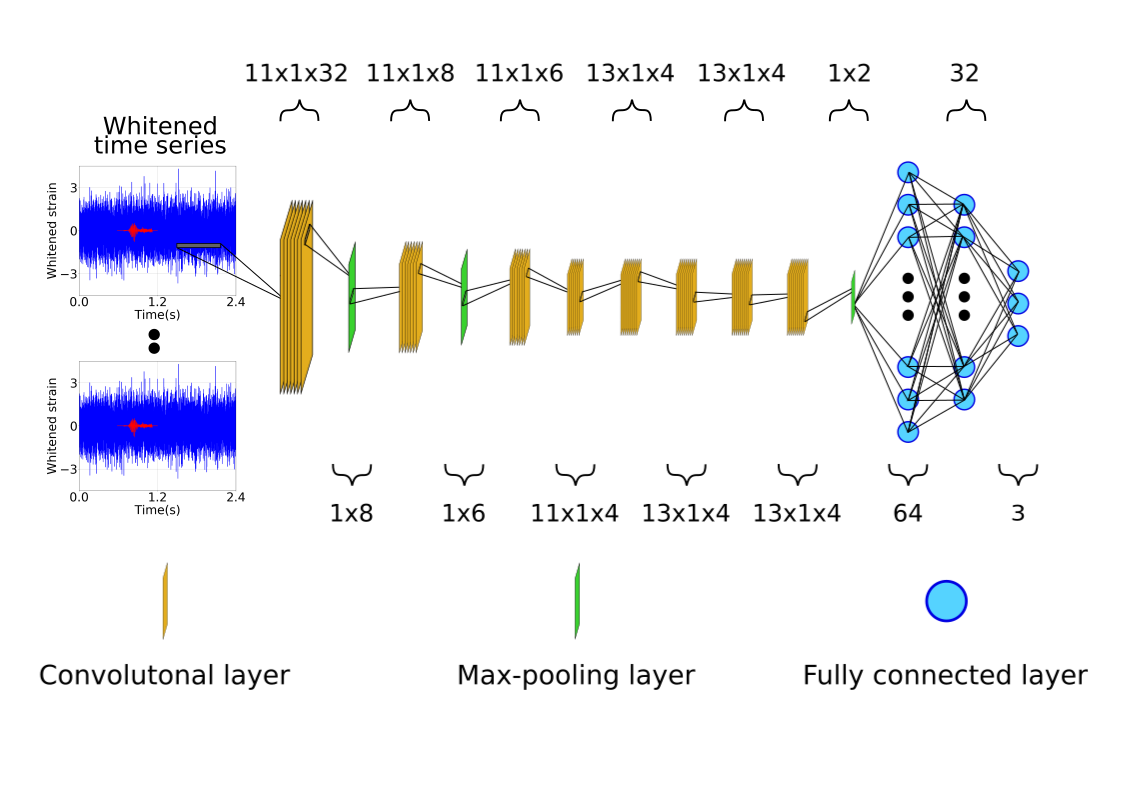
Figure 1: An illustration of the architecture of the CNN used in this paper for the detection and classification of CCSN GW signals in noisy data. The CNN consists of $8$ convolutional layers, $3$ max-pooling layers and $3$ fully connected layer including the output layer. The input layer takes the simulated time series of the detectors as input, feeding through the CNN. The CNN will output three probabilities at the last layer. The numbers above or below each layer indicate the kernal size of the layer. For example, the first convolutional layer has $11$ filters, each of which is $1$ by $32$ in size.

The problem we are trying to solve is a problem of multi-class classification, and hence the loss function employed for this work is the categorical cross-entropy abadi2016tensorflow , defined as

$$L(y,\hat{y})=-\sum^{M}_{j=1}\sum^{C}_{i=1}y_{ij}\log(\hat{y}_{ij}),$$ (1)

where $C$ is the number of the classes and $M$ is the number of the batch. For the $j^{\text{th}}$ sample and the $i^{\text{th}}$ class, $y_{ij}$ is the corresponding class value. It is equal to $1$ for the true class and $0$ otherwise. Similarly, $\hat{y}_{ij}$ is the predicted probability from the CNN for the $i^{\text{th}}$ class and the $j^{\text{th}}$ sample.

III Data

We establish a CNN for the purpose of distinguishing detector time series among three classes, i.e., magnetorotational signals $+$ background noise, neutrino-driven signals $+$ background noise, and pure background noise. For this purpose, it is necessary to prepare training, validation and testing data of these three classes. The training data is used for tuning the weights of the neurons in the layers in the CNN. Validating data is usually applied during training to verify that the CNN is learning the features inherent to the data and to prevent the CNN from over-fitting the training data. For a CNN that is not over-fitting, the value of the loss function will be close between the validation data and training data. Testing data is to test the performance of the trained CNN and applied after training has completed.

In our case, we define an input data sample as a set of simulated time series stacked together as a $k\times p$ matrix where $k$ is the number of detectors and $p$ the number of elements in the time series. To this end, we use simulated waveforms taken from the literature. The magnetorotational CCSN signals are taken from abdikamalov2014measuring ; dimmelmeier2008gravitational ; richers2017equation ^,. The simulations in abdikamalov2014measuring were focused on the dependence of the waveforms on the angular momentum distribution of the progenitors and provide us with 92 waveforms. In dimmelmeier2008gravitational , 136 waveforms are available from investigations into a variety of rotation rates and masses of the progenitors. The simulations in richers2017equation covered a parameter space of $18$ different equations of state and $98$ rotation profiles for a progenitor of $12\text{M}_{\odot}$ providing a total of $1824$ waveforms. All the simulations from the studies were based on 2D simulations of supernovae. It needs to be pointed out that as the authors in these studies were interested in the early stage of post-core bounce, and/or the effects of the equation of states on the GWs generated at core bounce, the simulations were only run for a short amount of time after core bounce. For example, the simulations in richers2017equation were only run for $50$ ms, and only approximately up to $10$ ms after core bounce were used.

For the neutrino-driven mechanism, we employ the waveforms from 10.1093mnrasstz990 ; kuroda2017correlated ; muller2012parametrized ; powell2019gravitational ; radice2019characterizing ; yakunin2015gravitational ; yakunin2017gravitational ; ott2009gravitational ; murphy2009model ; ott2013general ^,. The simulations in 10.1093mnrasstz990 ; kuroda2017correlated ; muller2012parametrized ; powell2019gravitational ; radice2019characterizing ; yakunin2017gravitational ; ott2013general were from 3D modelling of the supernovae while the simulations in yakunin2015gravitational ; ott2009gravitational ; murphy2009model were 2D. These simulations cover a wide range of progenitor masses from $9\text{M}_{\odot}$ to $60\text{M}_{\odot}$ and the specific progenitor masses of the simulations are shown in Table 2. Examples of the waveforms for both mechanisms are shown in Figs. 2 and 3.

Table 2: Waveforms

	Mechanism	Mass ($\text{M}_{\odot}$)	No.
Abdikamalov abdikamalov2014measuring	M	12.0	92
Dimmelmeier dimmelmeier2008gravitational	M	11.2,15.0,20.0,40.0	136
Richers richers2017equation	M	12.0	1824
Andresen 10.1093mnrasstz990	N	15.0	6
Kuroda kuroda2017correlated	N	11.2,15.0	2
Muller muller2012parametrized	N	15.0,20.0	6
Murphy murphy2009model	N	12.0,15.0,20.0,40.0	16
Ott1 ott2009gravitational	N	15.0	2
Ott2 ott2013general	N	27.0	8
Powell powell2019gravitational	N	$3.5^{*}$,18.0	2
Radice radice2019characterizing	N	9,10,11,12,13,19,25,60	8
Yakunin1 yakunin2015gravitational	N	12,15,20,25	4
Yakunin2 yakunin2017gravitational	N	15	1

• The mass ranges and mechanisms of the progenitors of the simulated waveforms used in this work. The first column refers to the studies. Mechanism indicates the explosion mechanism for the waveforms, with M for the magnetorotational mechanism and N for the neutrino-driven mechanism. Mass refers to the mass, in units of solar mass, of the progenitors in the simulations. No. means the number of waveforms available from the study. All masses are the masses of the stars at zeros age unless indicated otherwise.
  ^∗ Mass of a star in a binary system with an initial helium mass of $3.5\text{M}_{\odot}$

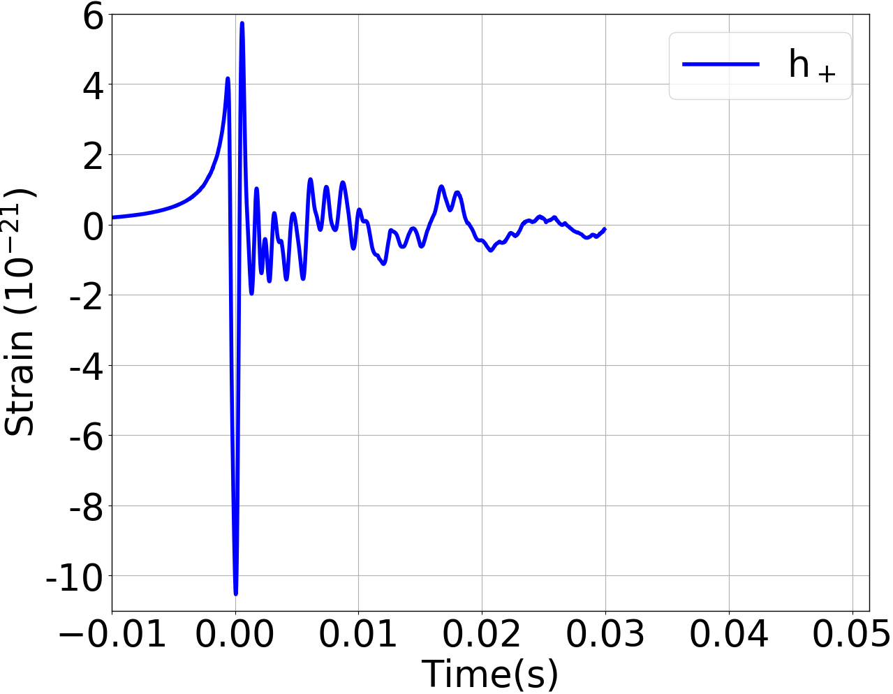
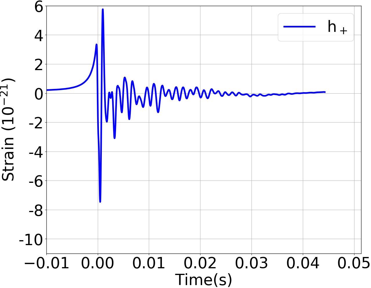
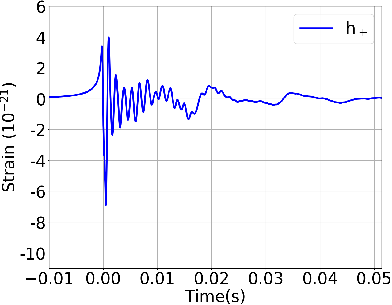
Figure 2: Examples of simulated waveforms for which the explosion is modelled by the magnetorotational mechanism. The left panel shows a waveform from abdikamalov2014measuring . The progenitor is $12\text{M}_{\odot}$ with differential rotation parameter $A=10^{4}~{}\text{km}$. The initial angular velocity at the core $\Omega_{c}$ is $5.0~{}\text{rads/s}$. The middle panel shows a waveform from dimmelmeier2008gravitational . The simulation corresponds to a progenitor of $15\text{M}_{\odot}$ with $A=10^{5}$ km and $\Omega_{c}=4.56~{}\text{rads/s}$. The right panel shows a waveform from richers2017equation where the progenitor is $12\text{M}_{\odot}$, $A$ and $\Omega_{c}$ are $10^{4}$ km and $3.0~{}\text{rad/s}$ respectively. In all panels, only the $h_{+}$ polarisations are shown because the simulations are axis-symmetric or 2D, and therefore described by only one polarisation. The sources are assumed to be at a distance of $10$ kpc. The x-axes show the time after core bounce.

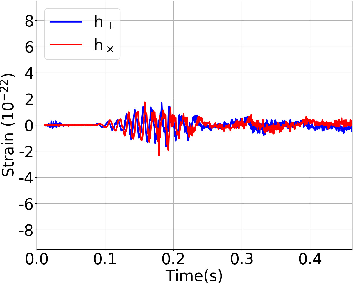
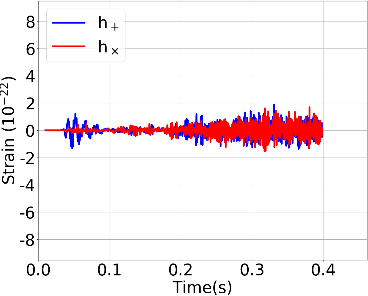
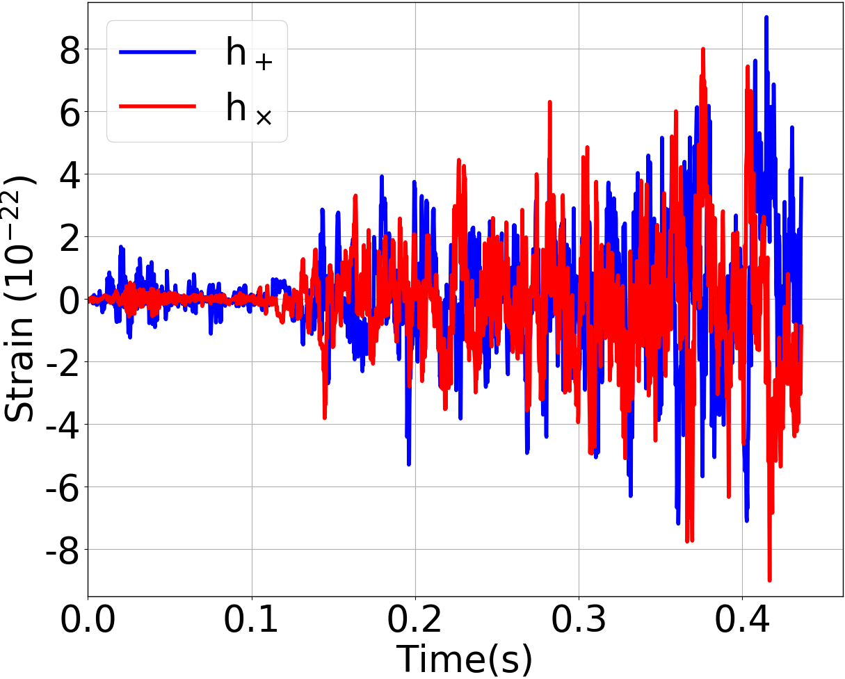
Figure 3: Examples of simulated waveforms for which the explosion mechanism is modelled by the neutrino-driven mechanism. From the left to the right, the panels show waveforms from 10.1093mnrasstz990 ; radice2019characterizing ; yakunin2017gravitational , with progenitors of masses equal to $15\text{M}_{\odot}$, $15\text{M}_{\odot}$ and $60\text{M}_{\odot}$ respectively. The sources are assumed to be at $10$ kpc from earth. The x-axes show the time after core bounce.

Introducing waveforms from a variety of studies introduces a distribution of the waveforms that covers a larger parameter space, making the data samples harder for the CNN to learn. As a result, the performance of the trained CNN on the testing samples may appear to be worse than that if the data were generated using only a subset of the waveforms. However, a larger parameter space provides the advantage of forcing the CNN to learn the features common among the waveforms rather than simply a subset of the waveforms. The trained network can thus perform better when presented with waveforms with unexpected features, which is more likely in reality.

Since the waveforms are generated at various distances, sampling rates and durations, it is necessary to normalise the waveforms before they can be used for the generation of the time-series. To do this, we first scale the amplitudes of the waveforms by moving the sources to $10$ kpc from earth. We then ensure that the sampling rate are identical for all the waveforms by down sampling them to a pre-selected sampling rate of $4096$Hz. The longest duration $\tau$ among the waveforms is then identified and each of the remaining waveforms is padded with zeros to this duration. To introduce as few artefacts as possible, a high pass filter with a low cut-off frequency equal to $11$Hz and a tukey window ($\alpha=0.08$) are applied prior to the zero padding.

To balance the difference in the number of waveforms between the two mechanisms in the training, validation and testing data set, $36$ exact copies of each neutrino-driven waveform are made. This will make the ratio of the waveforms modelled by the two mechanisms close to 1, while does not change the ratio of the waveforms from different studies modelled by the neutrino-driven mechanism. This means each waveform in the neutrino-driven mechanism will have equal representations in the data set, and waveforms from different mechanisms will have equal representation. After this procedure, the simulated waveforms are then $\mathbb{S}(t)=\{\mathbb{s}_{1}(t),\mathbb{s}_{2}(t),...,\mathbb{s}_{m}(t)\}$, where $m$ is the number of the waveforms and $\mathbb{s}_{q}$ is the $q^{\text{th}}$ waveform, defined by,

$$\mathbb{s}_{q}(t)=\left(\begin{array}[]{c}h_{q}^{+}(t)\\ h_{q}^{\times}(t)\end{array}\right),$$ (2)

where $h_{q}^{+}(t)$ and $h_{q}^{\times}(t)$ are the two polarisations of the waveform and $t$ is the time. In this work, we assume a fixed GPS time when generating the training/validation/testing data. At this GPS time, the value of $t$ is zero. As mentioned, some of the waveforms used in the work are generated with the simulations being axisymmetric, in which case the waveforms are entirely described by one polarisation $h_{q}^{+}(t)$. The corresponding $h_{q}^{\times}(t)$ for these waveforms are defined as a vector of zeros. In this work, we perform simulations for distances equal to $10$, $20$, $30$, $40$, $50$, $60$, $80$, $100$, $150$ and $200$ kpc. If for a training procedure, the default distance $d_{\text{L}}$ of a waveform is not $10$ kpc, the amplitude are rescaled by the distance since the amplitude is inversely proportional to the distance.

The next step is to generate simulated time-series for the GW detectors in a network using $\mathbb{S}(t)$. Since the purpose of building a CNN is to categorise an input data sample into three exclusive classes, in total three types of time-series are generated. For the time series containing either a magnetorotational signal or a neutrino-driven signal, we start by selecting a waveform $\mathbb{s}_{q}$ from $\mathbb{S}(t)$. A random location of (right ascension, declination) $=(\alpha,\delta)$ in the sky is selected from a uniform distribution on $\alpha$ and a uniform distribution on $\sin\delta$. The relative delays in the arrival times of the signals at each detector are a function of the sky location and are also computed and applied to the selected waveform. The delay in arrival time between a detector and the centre of the earth is given by,

$$\Delta t=\frac{\mathbb{n}(\alpha,\delta)\cdot\mathbb{r}}{c},$$ (3)

where $\mathbb{n}(\alpha,\delta)$ is the propagation direction of the GW, $c$ is the speed of light, and $\mathbb{r}$ the location vector of the detector relative to the centre of the Earth. The resulting $j^{\text{th}}$ signal $\mathbb{h}_{j}(\alpha,\delta,t)$ received by the detector network is then described by,

$$\mathbb{h}_{j}(\alpha,\delta,t)=\mathbb{F}(\alpha,\delta,t)\times\mathbb{s}_{q}(t+\mathbb{\Delta t}),$$ (4)

where $\mathbb{F}(\alpha,\delta,t)$ is a matrix of which the elements are the antenna patterns of each detector in the network,

$$\mathbb{F}(\alpha,\delta,t)=\left(\begin{array}[]{cc}f_{1}^{+}(\alpha,\delta,t)~{}~{}f_{1}^{\times}(\alpha,\delta,t)\\ \vdots~{}~{}~{}~{}~{}~{}~{}~{}~{}~{}~{}~{}\vdots\\ f_{k}^{+}(\alpha,\delta,t)~{}~{}f_{k}^{\times}(\alpha,\delta,t)\\ \end{array}\right),$$ (5)

$f^{+}(\alpha,\delta,t)$ and $f^{\times}(\alpha,\delta,t)$ are the antenna pattern functions for the two polarizations and $k$ is the number of detectors as defined above. Next, we generate independent Gaussian noise $\mathbb{N}_{j}(T)=\{\mathbb{n}_{1j}(T),\mathbb{n}_{2j}(T),...,\mathbb{n}_{kj}(T)\}^{\prime}$ for each detector in the network using their respective power spectral densities. In the expression, $T$ is the time for the generated noise and should not be confused with the lower case $t$, which is the time for the waveforms. To make the simulated data as realistic as possible, we allow the start time of the signal in a data sample to vary. To do this, the duration of the generated noise $T_{\text{max}}$ is $1.6$ times longer than that of $\mathbb{h}_{j}(\alpha,\delta,t)$. A random number $p$ drawn from a uniform distribution on the range of $[0,P)$ will then be generated, where $P=T_{\text{max}}\times 18\%$ and $p$ determines where in the generated noise the signal will be placed, as given by,

$$\mathbb{d}_{j}(\alpha,\delta,T,p)=\\ \begin{cases}\mathbb{N}_{j}(T)~{}~{}~{}~{}~{}~{}~{}~{}~{}~{}~{}~{}~{}~{}~{}~{}~{}t<T_{\text{max}}p;\\ \mathbb{N}_{j}(T)+\mathbb{h}_{j}(\alpha,\delta,t)~{}T_{\text{max}}p\leq T\leq\tau+T_{\text{max}}p;\\ \mathbb{N}_{j}(T)~{}~{}~{}~{}~{}~{}~{}~{}~{}~{}~{}~{}~{}~{}~{}~{}~{}t>\tau+T_{\text{max}}p,\\ \end{cases}$$ (6)

where $\tau$ is defined in section III. This will avoid the possibility that the CNN learns the human artefact instead of common features of the waveforms by having the signals always starting at the same place. For each time-series of the background noise class, independently simulated Gaussian background noise of the same duration as that of the other classes are generated using the same power spectrum density for each detector in the network. This means a data sample for this class is defined as,

$$\mathbb{d}_{j}(T)=\mathbb{N}_{j}(T).$$ (7)

As a general rule, the performance of a CNN can always be enhanced by increasing the volume of training data. Therefore we augment our data set by iterating over $\mathbb{S}(t)$ until for each waveform in $\mathbb{S}(t)$, we have $31$ data samples $\mathbb{d}$ generated using the procedure described above. This step is essential for the CNN to learn the features of the waveforms and to identify them effectively under different noise scenarios and starting times. After that, we generate independent noise realisations for the background noise class. The entire data set $\mathbb{D}$ has roughly $l=1.8\times 10^{5}$ data samples, where each of the 3 classes contains approximately $6\times 10^{4}$ data samples. In Fig. 4, we show a representative example of a pre-processed input time-series for a single detector. A data sample consists of such a time-series containing a signal from the same source or simply background noise from all the detectors in the network. The data samples are then split into 3 groups, with $1\times 10^{4}$ samples being randomly selected for validation, $10\%$ of the remainder for testing and $90\%$ for training. When the training is finished for a dataset generated at a given distance, the above described procedure will be repeated for another distance with a different CNN of the same architecture until the training for all distances have been carried out for a GW detector network. The entire procedure is then repeated for another GW detector network. As mentioned in the introduction, the CNN will be trained for the two networks of GW detectors presented in Table 3. For the remaining of the paper, we will use their acronyms to refer to the networks, i.e., HLVK and H+L+VK.

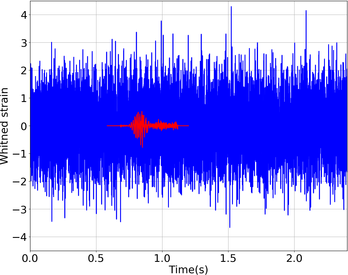
Figure 4: A representative example of the simulated time-series used to train/validate/test the CNN. The blue shows a whitened time-series with a signal added to Gaussian noise generated using the power spectral density of aLIGO. The red curve shows the same whitened signal free of noise. The original waveform is shown in Fig. 3. The source is at a distance of $10$ kpc from earth.

Table 3: Detector networks

Network	Detector	Acronym
1	aLIGO Hanford aasi2015advanced	HLVK
	aLIGO Livingston
	AdVirgo acernese2014advanced
	KAGRA aso2013interferometer
2	LIGO A+ Hanford miller2015prospects ; LIGOW	H+L+VK
	LIGO A+ Livingston
	AdVirgo
	KAGRA

• The networks of detectors used in this work.

IV Result and discussion

After the CNN is trained, we can estimate its performance using the testing samples and the results of which are presented in this section. By applying the trained network to the testing samples, the CNN will output values of statistics to each of the testing samples. Since we have knowledge of the true class associated with the testing samples, it is possible to construct the receiver operator characteristic (ROC) curves. The ROC curve is one of the most commonly used and convenient ways to determine the classification performance of a CNN or equivalent signal detection algorithm. A ROC shows the performance of a classifying model by defining the true alarm probability (TAP) as a function of the false alarm probability (FAP). Since ROC curves are usually plotted for models distinguishing between two classes, for a multi-class classification problem, a ROC for a class should be viewed as the class versus the others. This means in this context, FAP means the fraction of samples from other classes misidentified as a sample from the class the ROC is associated with. The TAP is identical to that of a two-class classification problem and indicates the fraction of samples correctly identified. For a given FAP, a model with a higher TAP is considered more capable than a model with a lower TAP.

In Fig. 5, we show the ROCs for both of the CCSN mechanisms and GW detector networks tested in this work. For simplicity, we show only the results for three distances, namely, $20$, $60$ and $100$ kpc. For all the distances tested, the CNN achieves a higher TAP for any given FAPs for magnetorotational than neutrino-driven signals. That is not surprising as the intrinsic amplitudes for magnetorotational signals are higher than those of neutrino-driven signals.

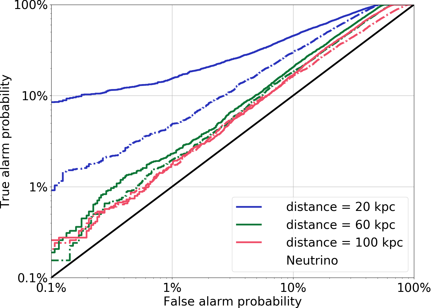
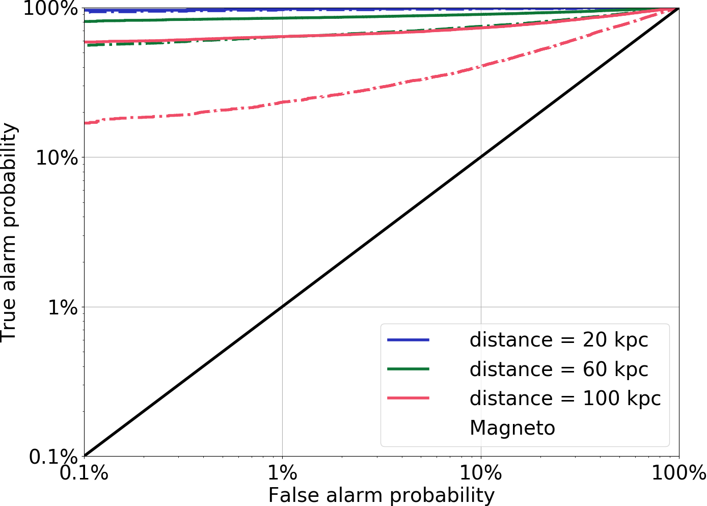
Figure 5: ROC curves showing the classification performance of the CNN for CCSN signals of different explosion mechanisms at three distances, $20$, $60$, and $100$ kpc. The left panel shows the results for the neutrino-driven mechanism, while the panel on the right shows those for the magnetorotational mechanism. In both panels, the solid lines are for the network H+L+VK, while the dashed lines are for HLVK. The black diagonal lines in both plots indicate the worst scenario where a model has zero ability in distinguishing its input.

We also show the classification efficiency of the CNN as a function of distance. This is done by fixing the FAP and plotting the TAP. The results for three chosen FAPs values are shown in Fig. 6. In this figure, a similar trend is seen that magnetorotational signals are easier for the CNN to identify than neutrino-driven signals at a given distance. For magnetorotational signals from sources located at $50$ kpc and a FAP of $10\%$, the CNN achieves a TAP of $94\%$ and $82\%$ for the networks H+L+VK and HLVK respectively. At more restrict FAPs such as $0.1\%$, the CNN still achieves TAPs $86\%$ and $68\%$ for sources at the same distance for the two networks respectively. For sources that are located at a slightly further distance of $60$ kpc, both networks achieve a TAP of close to or larger than $80\%$ at a FAP of $10\%$. Such a range includes distances associated with the Large and Small Magellanic Clouds and covers the satellite galaxies in between karachentsev2004catalog ; belokurov2007cats . For sources at $100$ kpc, the TAPs are close to or larger than $60\%$ for H+L+VK for all chosen FAPs values, and is $73\%$ if the FAP is $10\%$. Even for sources at $150$ and $200$ kpc, the TAPs are $54\%$ and $38\%$ respectively for the same FAP, indicating that with such a GW network, it is possible to detect magnetorotational CCSN signals out to such a distance. On the other hand, it is more difficult for the CNN to detect and classify the neutrino-driven signals, due to their weaker amplitudes. Nonetheless, for sources at $10$ kpc, the CNN achieves a TAP of $76\%$ and $55\%$ for H+L+VK and HLVK respectively if the FAP is $10\%$. This means that for a GW from a Galactic CCSN signal it is possible to detect and classify it with either of these GW detector networks.

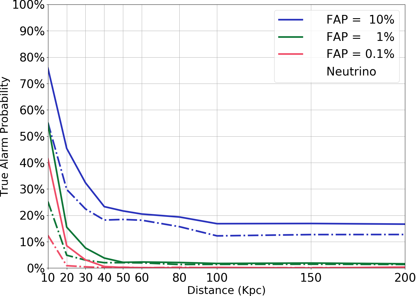
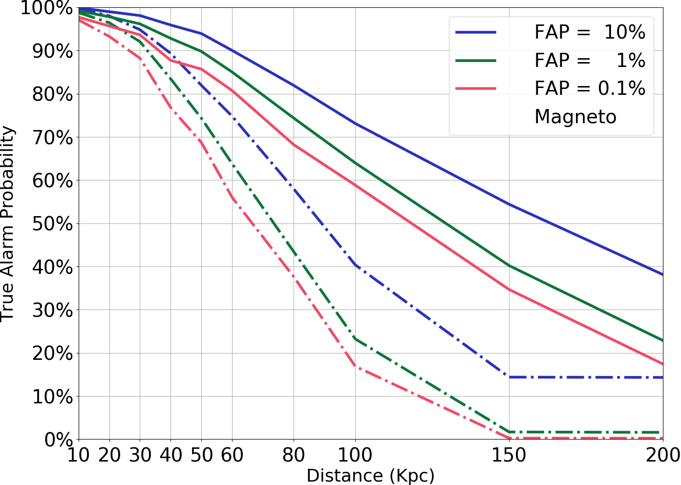
Figure 6: Efficiency curves showing the classification ability of the CNN as a function of distance for both mechanisms and networks. The left panel shows the results for the neutrino-driven mechanism, while the right shows those for the magnetorotational mechanism. In both panels, the solid lines show the results for the network H+L+VK, and the dashed lines for HLVK. Three FAPs values are chosen, blue for FAP $=10\%$, green for FAP $=1\%$, red for FAP $=0.1\%$.

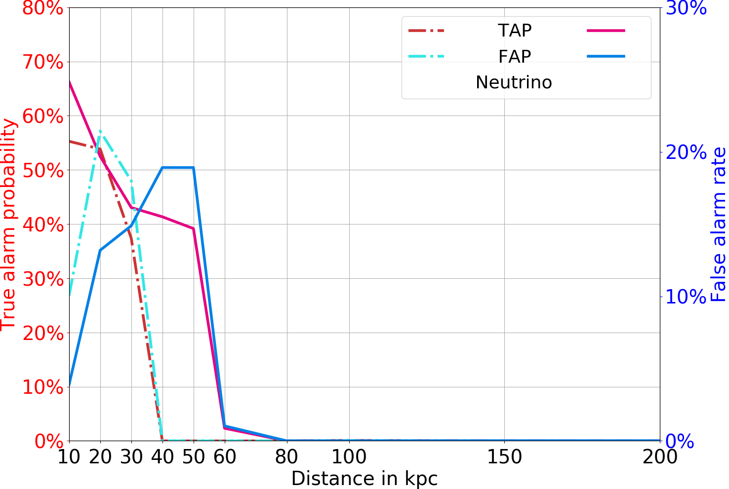
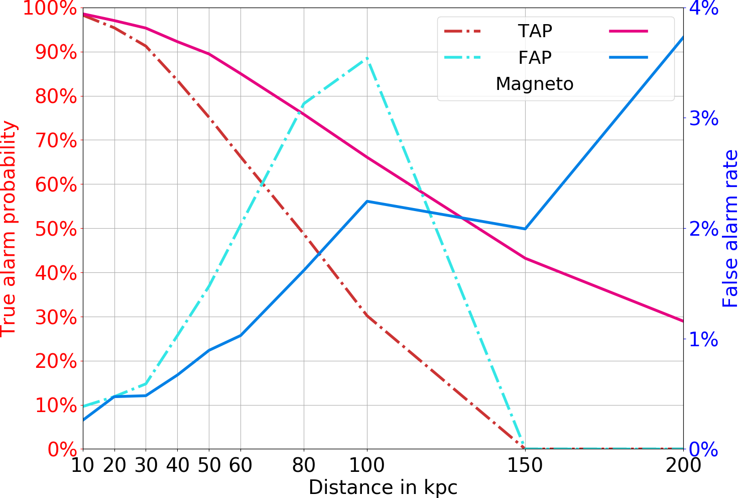
Figure 7: Efficiency curves showing the ability of the CNN in distinguishing input data with a fixed decision threshold $(50\%)$, and their corresponding FAPs and TAP. The left panel shows the results for the neutrino-driven mechanism, and the right shows that for the magnetorotational mechanism. In both panels, the solid lines show the TAPs and FAPs for the network H+L+VK, and the dashed lines show those for HLVK.

In practice, since the output of a CNN is probabilities indicating how likely the input belongs to each of the classes, it may be desired to set a threshold probability on which the decision whether the input belong to a class is made. For example, an input will be assigned into a certain class if the corresponding probability is larger than the pre-selected threshold probability. In such a scenario, the FAP and TAP would be affected by the choice of the threshold. We show such a result in Fig. 7, where we employed a threshold probability of $50\%$. This value is chosen because for lower values, there could be more than a class with predicted probabilities from the CNN larger than the threshold, while higher values could potentially rule out inputs that may otherwise be correctly identified. For H+L+VK and magnetorotational signals at $10$ kpc, the TAP is $99\%$. If the distance is extended to $80$ kpc, the TAP is still close to $80\%$. For the largest distances tested in this work, $150$ and $200$ kpc, the TAPs are $43\%$ and $29\%$ respectively. For HLVK, the TAP is $98\%$ and $49\%$ for sources at $10$ and $80$ kpc respectively. For all distances, the CNN maintains a FAP no larger than $4\%$ for both networks regarding magnetorotational waveforms. For neutrino-driven signals, we show that H+L+VK has a TAPs of $66\%$ at $10$ kpc while it is $55\%$ at $10$ kpc for HLVK. Both of the networks have FAPs close to or less than $20\%$. It should be noted that the results presented in this section are averaged over all the data samples in the testing samples. The performance on any individual waveform may vary depending on the morphology and the amplitudes of the waveform.

V Waveforms Excluded from Training

The previous section proves that using a CNN, it is possible to detect and classify CCSN waveforms if appropriate waveforms have been used to train the CNN. However, in reality, it is likely that the GWs from a CCSN may only be partially similar to the simulated waveforms, while having some other features that are different or even unexpected. A CNN that is only capable of recognising waveforms with which it is familiar may prove to be not entirely applicable. Therefore, we apply our trained CNN to waveforms from other studies that were not used during the training. Similar to the procedure used in roma2019astrophysics , we take the waveforms R3E1AC and R4E1FC_L from scheidegger2010influence as the test waveforms for the magnetorotational mechanism. The test waveforms for the neutrino-driven mechanisms are $\text{s}20$ from andresen2017gravitational and SFHx from kuroda2016new . These waveforms are shown in Fig. 8. The test waveforms in this section should not be confused with the testing samples in Sec. IV, which are randomly drawn from the same distribution as the training samples.

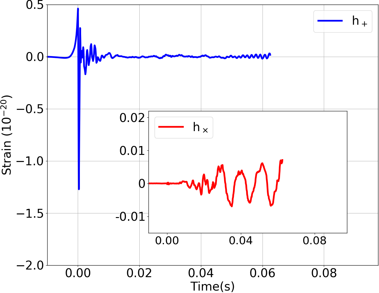
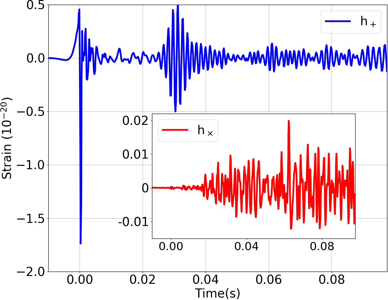
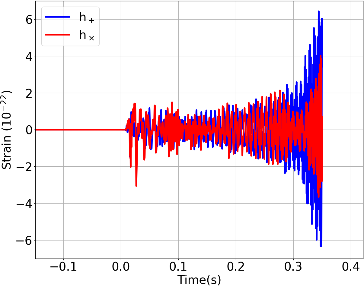
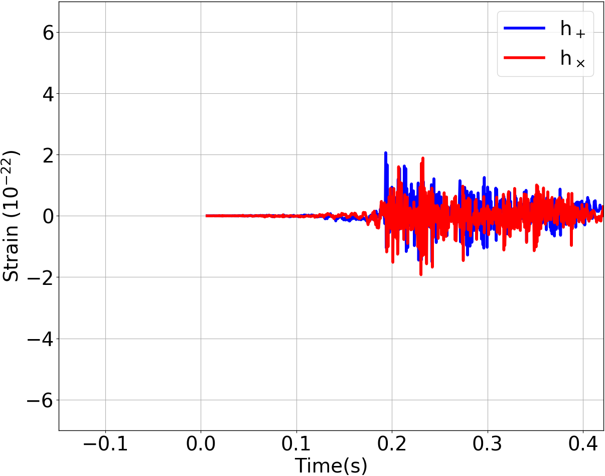
Figure 8: The waveforms excluded from the training session of the CNN and used as an extra test for the performance of the trained CNN. The top panels show the waveforms R3E1AC(left) and R4E1FC_L(right), modelled by the magnetorotational mechanism. The inset plots show the $h_{\times}$ polarisations of the waveform, which are at least one order of magnitude weaker than the $h_{+}$ polarisations. The waveforms shown in the bottom panels are SFHx(left) and $\text{s}20$(right), modelled by the neutrino-driven mechanism. Shown in the x-axes are the time after core bounce.

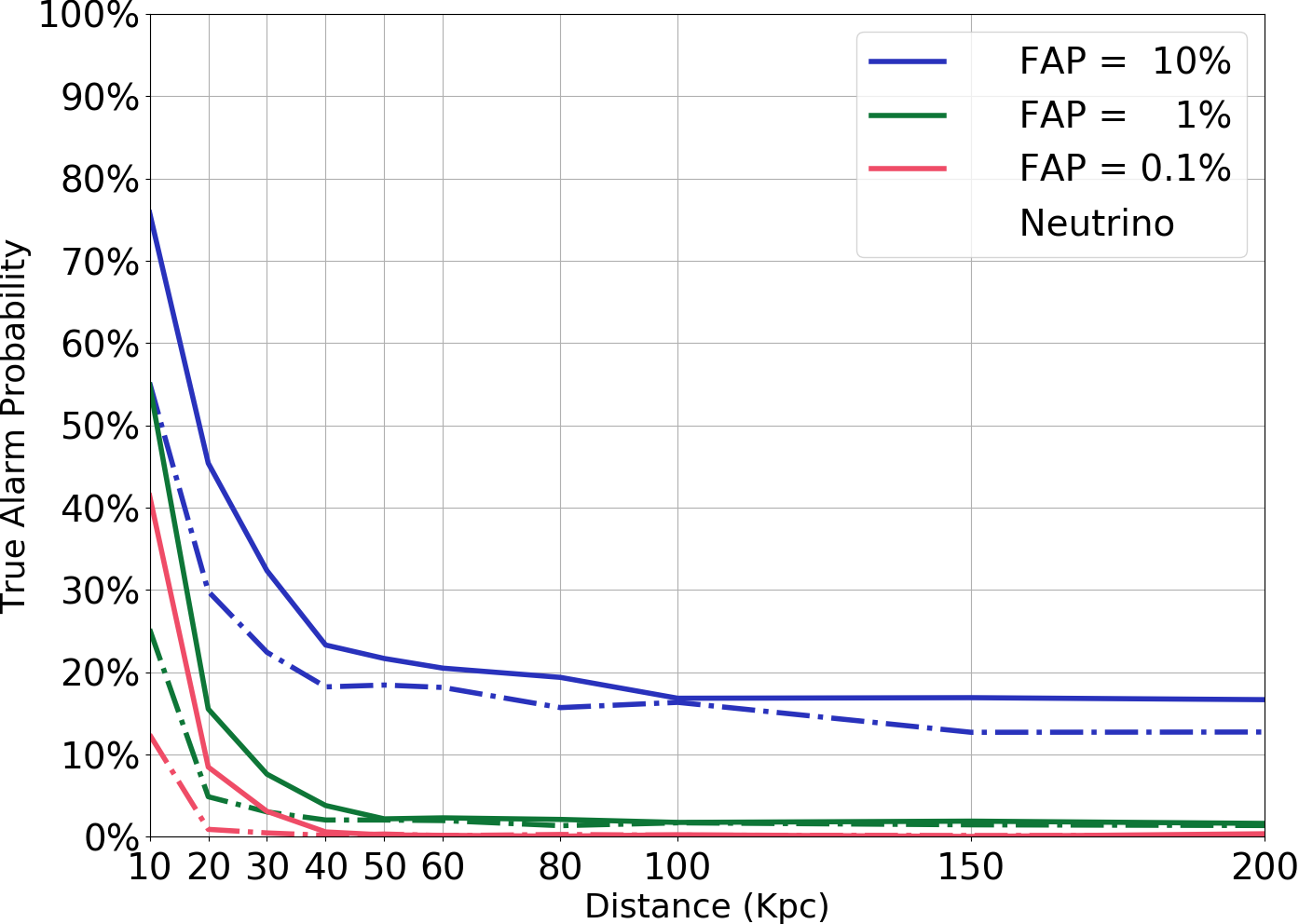
Figure 9: Efficiency curves showing the ability of the CNN in distinguishing input data. The upper panel shows the results for the the waveforms SFHx and $\text{s}20$ (neutrino-driven mechanism), and the lower panel shows that for the waveforms R3E1AC and R4E1FC_L (the magnetorotational mechanism). In both panels, the solid lines show the TAPs and FAPs for H+L+VK, and the dashed lines show those for HLVK. The waveforms have not been used for the training of the CNN.

Using the procedure described in Sec. III, we generate $1200$ samples for each distance and therefore each class has $400$ samples. The performance of the CNN on the test waveforms is shown in Fig. 9. For waveforms R3E1AC and R4E1FC_L at $50$ kpc and a FAP of $10\%$, the CNN achieves a TAP of $87\%$ with H+L+VK and $59\%$ with HLVK respectively. At $60$ kpc, the TAPs drops slightly to $83\%$ and $52\%$ respectively. This indicates that with the CNN, it is possible to detect these waveforms from sources that are at distances consistent with the Large and Small Magellanic Clouds. For waveforms $\text{s}20$ and SFHx, the TAPs are $93\%$ and $70\%$ for the two networks if the sources are at $10$ kpc and the FAP is $10\%$. The efficiency for the waveforms $\text{s}20$ and SFHx is noticeably higher than that for the neutrino-driven mechanism in Fig. 6 for the same distance. This is because as mentioned before, the detection and classification efficiency in Fig. 6 are the results averaged over the testing samples. It is possible that individual waveforms may be easier for the CNN to detect.

VI Conclusion

We have demonstrated that a CNN can be applied for the purpose of distinguishing GW detector time-series among pure background noise and CCSN explosion mechanisms. We have trained the CNN using $1.8\times 10^{5}$ samples of simulated time series for each distance at a number of distances from $10$ kpc to $200$ kpc. The data samples for each class consisted of approximately $4\times 10^{5}$ samples.

We have shown that with a GW detector network of HLVK, when the FAP was $10\%$, once trained, a CNN could achieve a TAP close to $80\%$ for magnetorotational signals from sources at $60$ kpc. Using a network of H+L+VK, we showed that the TAP is increased to $91\%$. Both the Large and Small Magellanic Clouds are within this distance. If the distance is extended to $150$ or $200$ kpc, a TAP of $54\%$ or $38\%$ respectively are still achievable for H+L+VK, indicating the small possibility of detections within such distances.

For the neutrino-driven mechanism, the weaker amplitudes of the waveforms result in lower TAPs at the same distances. For sources at $10$ kpc, the trained CNN, with a FAP of $10\%$, achieved a TAP of $55\%$ and $76\%$ for HLVK and H+L+VK respectively. This indicates a Galactic CCSN event would likely be detectable.

We used four waveforms that were not used for the training of the CNN to test the performance of the CNN in a more realistic situation. We found that for waveforms R3E1AC and R4E1FC_L from sources at $60$ kpc, the TAPs are $83\%$ and $52\%$ for H+L+VK and HLVK respectively. For waveforms $\text{s}20$ and SFHx, the TAPs are $93\%$ and $70\%$ for the two networks respectively. All at FAP of $10\%$. The results prove the possibility of using a CNN as a tool for the detection and classification of CCSN GW signals.

VII ACKNOWLEDGEMENTS

We would like to thank Jade Powell and Marek Szczepanczyk for their constructive comments on the paper. We would also like to thank that for the computational resources. I.S.H. and C.M. are supported by the Science and Technology Research Council (grant No. ST/L000946/1) and the European Cooperation in Science and Technology (COST) action CA17137.

References

- (1) Benjamin P Abbott, Richard Abbott, TD Abbott, et al. Observation of gravitational waves from a binary black hole merger. Physical review letters, 116(6):061102, 2016.
- (2) Benjamin P Abbott, R Abbott, TD Abbott, et al. Gw151226: observation of gravitational waves from a 22-solar-mass binary black hole coalescence. Physical review letters, 116(24):241103, 2016.
- (3) Benjamin P Abbott, R Abbott, TD Abbott, et al. Gw170608: Observation of a 19 solar-mass binary black hole coalescence. The Astrophysical Journal Letters, 851(2):L35, 2017.
- (4) Benjamin P Abbott, R Abbott, TD Abbott, et al. Gw170814: a three-detector observation of gravitational waves from a binary black hole coalescence. Physical review letters, 119(14):141101, 2017.
- (5) Benjamin P Abbott, Rich Abbott, TD Abbott, et al. Gw170817: observation of gravitational waves from a binary neutron star inspiral. Physical Review Letters, 119(16):161101, 2017.
- (6) Benjamin P Abbott, R Abbott, TD Abbott, et al. Gravitational waves and gamma-rays from a binary neutron star merger: Gw170817 and grb 170817a. The Astrophysical Journal Letters, 848(2):L13, 2017.
- (7) Benjamin P Abbott, Richard Abbott, TD Abbott, et al. Multi-messenger observations of a binary neutron star merger. Astrophys. J. Lett, 848(2):L12, 2017.
- (8) Yoichi Aso, Yuta Michimura, Kentaro Somiya, et al. Interferometer design of the kagra gravitational wave detector. Physical Review D, 88(4):043007, 2013.
- (9) Kentaro Somiya. Detector configuration of kagra–the japanese cryogenic gravitational-wave detector. Classical and Quantum Gravity, 29(12):124007, 2012.
- (10) Benjamin P Abbott, R Abbott, TD Abbott, et al. Prospects for observing and localizing gravitational-wave transients with advanced ligo, advanced virgo and kagra. Living Reviews in Relativity, 21(1):3, 2018.
- (11) Junaid Aasi, BP Abbott, Richard Abbott, et al. Advanced ligo. Classical and quantum gravity, 32(7):074001, 2015.
- (12) F Acernese, M Agathos, K Agatsuma, et al. Advanced virgo: a second-generation interferometric gravitational wave detector. Classical and Quantum Gravity, 32(2):024001, 2014.
- (13) SE Gossan, Patrick Sutton, A Stuver, et al. Observing gravitational waves from core-collapse supernovae in the advanced detector era. Physical Review D, 93(4):042002, 2016.
- (14) Benjamin P Abbott, Richard Abbott, TD Abbott, et al. First targeted search for gravitational-wave bursts from core-collapse supernovae in data of first-generation laser interferometer detectors. Physical Review D, 94(10):102001, 2016.
- (15) BP Abbott, R Abbott, TD Abbott, et al. An optically targeted search for gravitational waves emitted by core-collapse supernovae during the first and second observing runs of advanced ligo and advanced virgo. arXiv preprint arXiv:1908.03584, 2019.
- (16) Katsuhiko Sato and Hideyuki Suzuki. Analysis of neutrino burst from the supernova 1987a in the large magellanic cloud. Physical review letters, 58(25):2722, 1987.
- (17) E Baron and J Cooperstein. The effect of iron core structure on supernovae. The Astrophysical Journal, 353:597–611, 1990.
- (18) Hans Albrecht Bethe. Supernova mechanisms. Reviews of Modern Physics, 62(4):801, 1990.
- (19) Evan O’Connor and Christian D Ott. Black hole formation in failing core-collapse supernovae. The Astrophysical Journal, 730(2):70, 2011.
- (20) Hans A Bethe and James R Wilson. Revival of a stalled supernova shock by neutrino heating. The Astrophysical Journal, 295:14–23, 1985.
- (21) Hans-Thomas Janka. Explosion mechanisms of core-collapse supernovae. Annual Review of Nuclear and Particle Science, 62:407–451, 2012.
- (22) Kei Kotake, Kohsuke Sumiyoshi, Shoichi Yamada, et al. Core-collapse supernovae as supercomputing science: A status report toward six-dimensional simulations with exact boltzmann neutrino transport in full general relativity. Progress of Theoretical and Experimental Physics, 2012(1), 2012.
- (23) Anthony Mezzacappa, Stephen W Bruenn, Eric J Lentz, et al. Two-and three-dimensional multi-physics simulations of core collapse supernovae: A brief status report and summary of results from the” oak ridge” group. arXiv preprint arXiv:1405.7075, 2014.
- (24) Tomoya Takiwaki, Kei Kotake, and Yudai Suwa. Three-dimensional simulations of rapidly rotating core-collapse supernovae: finding a neutrino-powered explosion aided by non-axisymmetric flows. Monthly Notices of the Royal Astronomical Society: Letters, 461(1):L112–L116, 2016.
- (25) Alexander Summa, Hans-Thomas Janka, Tobias Melson, and Andreas Marek. Rotation-supported neutrino-driven supernova explosions in three dimensions and the critical luminosity condition. The Astrophysical Journal, 852(1):28, 2018.
- (26) Stephen W Bruenn, Eric J Lentz, W Raphael Hix, et al. The development of explosions in axisymmetric ab initio core-collapse supernova simulations of 12–25 stars. The Astrophysical Journal, 818(2):123, 2016.
- (27) H-Th Janka, K Langanke, Andreas Marek, G Martínez-Pinedo, and B Müller. Theory of core-collapse supernovae. Physics Reports, 442(1-6):38–74, 2007.
- (28) Sean M Couch and Christian D Ott. The role of turbulence in neutrino-driven core-collapse supernova explosions. The Astrophysical Journal, 799(1):5, 2015.
- (29) John M Blondin, Anthony Mezzacappa, and Christine DeMarino. Stability of standing accretion shocks, with an eye toward core-collapse supernovae. The Astrophysical Journal, 584(2):971, 2003.
- (30) JM LeBlanc and JR Wilson. A numerical example of the collapse of a rotating magnetized star. The Astrophysical Journal, 161:541, 1970.
- (31) Adam Burrows, Luc Dessart, Eli Livne, Christian D Ott, and Jeremiah Murphy. Simulations of magnetically driven supernova and hypernova explosions in the context of rapid rotation. The Astrophysical Journal, 664(1):416, 2007.
- (32) Tomoya Takiwaki, Kei Kotake, and Katsuhiko Sato. Special relativistic simulations of magnetically dominated jets in collapsing massive stars. The Astrophysical Journal, 691(2):1360, 2009.
- (33) SG Moiseenko, GS Bisnovatyi-Kogan, and NV Ardeljan. A magnetorotational core-collapse model with jets. Monthly Notices of the Royal Astronomical Society, 370(1):501–512, 2006.
- (34) Philipp Mösta, Sherwood Richers, Christian D Ott, et al. Magnetorotational core-collapse supernovae in three dimensions. The Astrophysical Journal Letters, 785(2):L29, 2014.
- (35) SE Woosley and Alexander Heger. The progenitor stars of gamma-ray bursts. The Astrophysical Journal, 637(2):914, 2006.
- (36) S-C Yoon and Norbert Langer. On the evolution of rapidly rotating massive white dwarfs towards supernovae or collapses. Astronomy & Astrophysics, 435(3):967–985, 2005.
- (37) SE De Mink, N Langer, RG Izzard, Hugues Sana, and Alex de Koter. The rotation rates of massive stars: the role of binary interaction through tides, mass transfer, and mergers. The Astrophysical Journal, 764(2):166, 2013.
- (38) Samantha A Usman, Alexander H Nitz, Ian W Harry, et al. The pycbc search for gravitational waves from compact binary coalescence. Classical and Quantum Gravity, 33(21):215004, 2016.
- (39) Kipp Cannon, Romain Cariou, Adrian Chapman, et al. Toward early-warning detection of gravitational waves from compact binary coalescence. The Astrophysical Journal, 748(2):136, 2012.
- (40) Christian D Ott. The gravitational-wave signature of core-collapse supernovae. Classical and Quantum Gravity, 26(6):063001, 2009.
- (41) Kei Kotake. Multiple physical elements to determine the gravitational-wave signatures of core-collapse supernovae. Comptes Rendus Physique, 14(4):318–351, 2013.
- (42) Kei Kotake, Wakana Iwakami, Naofumi Ohnishi, and Shoichi Yamada. Stochastic nature of gravitational waves from supernova explosions with standing accretion shock instability. The Astrophysical Journal Letters, 697(2):L133, 2009.
- (43) Ik Siong Heng. Rotating stellar core-collapse waveform decomposition: a principal component analysis approach. Classical and Quantum Gravity, 26(10):105005, 2009.
- (44) Christian Röver, Marie-Anne Bizouard, Nelson Christensen, et al. Bayesian reconstruction of gravitational wave burst signals from simulations of rotating stellar core collapse and bounce. Physical Review D, 80(10):102004, 2009.
- (45) Jade Powell, Daniele Trifirò, Elena Cuoco, Ik Siong Heng, and Marco Cavaglià. Classification methods for noise transients in advanced gravitational-wave detectors. Classical and Quantum Gravity, 32(21):215012, 2015.
- (46) Jade Powell, Alejandro Torres-Forné, Ryan Lynch, et al. Classification methods for noise transients in advanced gravitational-wave detectors ii: performance tests on advanced ligo data. Classical and Quantum Gravity, 34(3):034002, 2017.
- (47) Sofia Suvorova, Jade Powell, and Andrew Melatos. Reconstructing gravitational wave core-collapse supernova signals with dynamic time warping. Physical Review D, 99(12):123012, 2019.
- (48) J Logue, CD Ott, IS Heng, P Kalmus, and JHC Scargill. Inferring core-collapse supernova physics with gravitational waves. Physical Review D, 86(4):044023, 2012.
- (49) William J Engels, Raymond Frey, and Christian D Ott. Multivariate regression analysis of gravitational waves from rotating core collapse. Physical Review D, 90(12):124026, 2014.
- (50) TZ Summerscales, Adam Burrows, Lee Samuel Finn, and Christian D Ott. Maximum entropy for gravitational wave data analysis: Inferring the physical parameters of core-collapse supernovae. The Astrophysical Journal, 678(2):1142, 2008.
- (51) S Klimenko, G Vedovato, M Drago, et al. Method for detection and reconstruction of gravitational wave transients with networks of advanced detectors. Physical Review D, 93(4):042004, 2016.
- (52) Malik Rakhmanov. Rank deficiency and tikhonov regularization in the inverse problem for gravitational-wave bursts. Classical and Quantum Gravity, 23(19):S673, 2006.
- (53) Kazuhiro Hayama, Soumya D Mohanty, Malik Rakhmanov, and Shantanu Desai. Coherent network analysis for triggered gravitational wave burst searches. Classical and Quantum Gravity, 24(19):S681, 2007.
- (54) Alex Krizhevsky, Ilya Sutskever, and Geoffrey E Hinton. Imagenet classification with deep convolutional neural networks. In Advances in neural information processing systems, pages 1097–1105, 2012.
- (55) Ian Goodfellow, Jean Pouget-Abadie, Mehdi Mirza, et al. Generative adversarial nets. In Z. Ghahramani, M. Welling, C. Cortes, N. D. Lawrence, and K. Q. Weinberger, editors, Advances in Neural Information Processing Systems 27, pages 2672–2680. Curran Associates, Inc., 2014.
- (56) Karen Simonyan and Andrew Zisserman. Very deep convolutional networks for large-scale image recognition. arXiv preprint arXiv:1409.1556, 2014.
- (57) Liang-Chieh Chen, George Papandreou, Iasonas Kokkinos, Kevin Murphy, and Alan L Yuille. Semantic image segmentation with deep convolutional nets and fully connected crfs. arXiv preprint arXiv:1412.7062, 2014.
- (58) Matthew D Zeiler and Rob Fergus. Visualizing and understanding convolutional networks. In European conference on computer vision, pages 818–833. Springer, 2014.
- (59) Christian Szegedy, Wei Liu, Yangqing Jia, et al. Going deeper with convolutions. In Proceedings of the IEEE conference on computer vision and pattern recognition, pages 1–9, 2015.
- (60) Igor Kononenko. Machine learning for medical diagnosis: history, state of the art and perspective. Artificial Intelligence in medicine, 23(1):89–109, 2001.
- (61) Joseph Redmon, Santosh Divvala, Ross Girshick, and Ali Farhadi. You only look once: Unified, real-time object detection. In Proceedings of the IEEE conference on computer vision and pattern recognition, pages 779–788, 2016.
- (62) Kaiming He, Xiangyu Zhang, Shaoqing Ren, and Jian Sun. Deep residual learning for image recognition. In Proceedings of the IEEE conference on computer vision and pattern recognition, pages 770–778, 2016.
- (63) Richard Zhang, Phillip Isola, and Alexei A Efros. Colorful image colorization. In European conference on computer vision, pages 649–666. Springer, 2016.
- (64) Andrej Karpathy and Li Fei-Fei. Deep visual-semantic alignments for generating image descriptions. In Proceedings of the IEEE conference on computer vision and pattern recognition, pages 3128–3137, 2015.
- (65) Guillaume Lample, Miguel Ballesteros, Sandeep Subramanian, Kazuya Kawakami, and Chris Dyer. Neural architectures for named entity recognition. arXiv preprint arXiv:1603.01360, 2016.
- (66) Nikhil Mukund, Sheelu Abraham, Shivaraj Kandhasamy, Sanjit Mitra, and Ninan Sajeeth Philip. Transient classification in ligo data using difference boosting neural network. Physical Review D, 95(10):104059, 2017.
- (67) Michael Zevin, Scott Coughlin, Sara Bahaadini, et al. Gravity spy: integrating advanced ligo detector characterization, machine learning, and citizen science. Classical and quantum gravity, 34(6):064003, 2017.
- (68) Daniel George, Hongyu Shen, and EA Huerta. Deep transfer learning: A new deep learning glitch classification method for advanced ligo. arXiv preprint arXiv:1706.07446, 2017.
- (69) Daniel George and EA Huerta. Deep learning for real-time gravitational wave detection and parameter estimation: Results with advanced ligo data. Physics Letters B, 778:64–70, 2018.
- (70) Hunter Gabbard, Michael Williams, Fergus Hayes, and Chris Messenger. Matching matched filtering with deep networks for gravitational-wave astronomy. Physical review letters, 120(14):141103, 2018.
- (71) P Astone, P Cerdá-Durán, I Di Palma, et al. New method to observe gravitational waves emitted by core collapse supernovae. Physical Review D, 98(12):122002, 2018.
- (72) Hunter Gabbard, Chris Messenger, Ik Siong Heng, Francesco Tonolini, and Roderick Murray-Smith. Bayesian parameter estimation using conditional variational autoencoders for gravitational-wave astronomy. arXiv e-prints, page arXiv:1909.06296, Sep 2019.
- (73) Ian Goodfellow, Yoshua Bengio, and Aaron Courville. Deep learning. MIT press, 2016.
- (74) John Miller, Lisa Barsotti, Salvatore Vitale, et al. Prospects for doubling the range of advanced ligo. Physical Review D, 91(6):062005, 2015.
- (75) B. Lantz, S. Danilishin, S. Hild, et al. Ligo instrument science white paper. 2018.
- (76) Sergei Klimenko, S Mohanty, Malik Rakhmanov, and Guenakh Mitselmakher. Constraint likelihood analysis for a network of gravitational wave detectors. Physical Review D, 72(12):122002, 2005.
- (77) Keiron O’Shea and Ryan Nash. An introduction to convolutional neural networks. arXiv preprint arXiv:1511.08458, 2015.
- (78) Yann LeCun, D Touresky, G Hinton, and T Sejnowski. A theoretical framework for back-propagation. In Proceedings of the 1988 connectionist models summer school, volume 1, pages 21–28. CMU, Pittsburgh, Pa: Morgan Kaufmann, 1988.
- (79) Nitish Srivastava, Geoffrey Hinton, Alex Krizhevsky, Ilya Sutskever, and Ruslan Salakhutdinov. Dropout: a simple way to prevent neural networks from overfitting. The journal of machine learning research, 15(1):1929–1958, 2014.
- (80) Martín Abadi, Ashish Agarwal, Paul Barham, et al. Tensorflow: Large-scale machine learning on heterogeneous distributed systems. arXiv preprint arXiv:1603.04467, 2016.
- (81) Ernazar Abdikamalov, Sarah Gossan, Alexandra M DeMaio, and Christian D Ott. Measuring the angular momentum distribution in core-collapse supernova progenitors with gravitational waves. Physical Review D, 90(4):044001, 2014.
- (82) Harald Dimmelmeier, Christian D Ott, Andreas Marek, and H-Thomas Janka. Gravitational wave burst signal from core collapse of rotating stars. Physical Review D, 78(6):064056, 2008.
- (83) Sherwood Richers, Christian D Ott, Ernazar Abdikamalov, Evan O’Connor, and Chris Sullivan. Equation of state effects on gravitational waves from rotating core collapse. Physical Review D, 95(6):063019, 2017.
- (84) H Andresen, E Müller, H-Th Janka, et al. Gravitational waves from 3D core-collapse supernova models: The impact of moderate progenitor rotation. Monthly Notices of the Royal Astronomical Society, 486(2):2238–2253, 04 2019.
- (85) Takami Kuroda, Kei Kotake, Kazuhiro Hayama, and Tomoya Takiwaki. Correlated signatures of gravitational-wave and neutrino emission in three-dimensional general-relativistic core-collapse supernova simulations. The Astrophysical Journal, 851(1):62, 2017.
- (86) E Müller, H-Th Janka, and A Wongwathanarat. Parametrized 3d models of neutrino-driven supernova explosions-neutrino emission asymmetries and gravitational-wave signals. Astronomy & Astrophysics, 537:A63, 2012.
- (87) Jade Powell and Bernhard Müller. Gravitational wave emission from 3d explosion models of core-collapse supernovae with low and normal explosion energies. Monthly Notices of the Royal Astronomical Society, 487(1):1178–1190, 2019.
- (88) David Radice, Viktoriya Morozova, Adam Burrows, David Vartanyan, and Hiroki Nagakura. Characterizing the gravitational wave signal from core-collapse supernovae. The Astrophysical Journal Letters, 876(1):L9, 2019.
- (89) Konstantin N Yakunin, Anthony Mezzacappa, Pedro Marronetti, et al. Gravitational wave signatures of ab initio two-dimensional core collapse supernova explosion models for 12–25 m⊙ stars. Physical Review D, 92(8):084040, 2015.
- (90) Konstantin N Yakunin, Anthony Mezzacappa, Pedro Marronetti, et al. The gravitational wave signal of a core collapse supernova explosion of a 15 star. arXiv preprint arXiv:1701.07325, 2017.
- (91) Jeremiah W Murphy, Christian D Ott, and Adam Burrows. A model for gravitational wave emission from neutrino-driven core-collapse supernovae. The Astrophysical Journal, 707(2):1173, 2009.
- (92) Christian D Ott, Ernazar Abdikamalov, Philipp Mösta, et al. General-relativistic simulations of three-dimensional core-collapse supernovae. The Astrophysical Journal, 768(2):115, 2013.
- (93) Igor D Karachentsev, Valentina E Karachentseva, Walter K Huchtmeier, and Dmitry I Makarov. A catalog of neighboring galaxies. The Astronomical Journal, 127(4):2031, 2004.
- (94) V Belokurov, Daniel B Zucker, NW Evans, et al. Cats and dogs, hair and a hero: a quintet of new milky way companions. The Astrophysical Journal, 654(2):897, 2007.
- (95) Vincent Roma, Jade Powell, Ik Siong Heng, and Raymond Frey. Astrophysics with core-collapse supernova gravitational wave signals in the next generation of gravitational wave detectors. Physical Review D, 99(6):063018, 2019.
- (96) S Scheidegger, R Käppeli, SC Whitehouse, T Fischer, and M Liebendörfer. The influence of model parameters on the prediction of gravitational wave signals from stellar core collapse. Astronomy & Astrophysics, 514:A51, 2010.
- (97) Haakon Andresen, Bernhard Müller, Ewald Müller, and H-Th Janka. Gravitational wave signals from 3d neutrino hydrodynamics simulations of core-collapse supernovae. Monthly Notices of the Royal Astronomical Society, 468(2):2032–2051, 2017.
- (98) Takami Kuroda, Kei Kotake, and Tomoya Takiwaki. A new gravitational-wave signature from standing accretion shock instability in supernovae. The Astrophysical Journal Letters, 829(1):L14, 2016.