Higher Anomalies, Higher Symmetries, and
Cobordisms III:
QCD Matter Phases Anew

Zheyan Wan¹ and Juven Wang<sup>2,3

1</sup>Yau Mathematical Sciences Center, Tsinghua University, Beijing 100084, China
²Center of Mathematical Sciences and Applications, Harvard University, Cambridge, MA 02138, USA
³School of Natural Sciences, Institute for Advanced Study, Einstein Drive, Princeton, NJ 08540, USA

We explore QCD₄ quark matter, the $\mu$-T (chemical potential-temperature) phase diagram, possible ’t Hooft anomalies, and topological terms, via non-perturbative tools of cobordism theory and higher anomaly matching. We focus on quarks in 3-color and 3-flavor on bi-fundamentals of SU(3), then analyze the continuous and discrete global symmetries and pay careful attention to finite group sectors. We input constraints from $T=CP$ or $CT$ time-reversal symmetries, implementing QCD on unorientable spacetimes and distinct topology. Examined phases include the high T QGP (quark-gluon plasma/liquid), the low T ChSB (chiral symmetry breaking), 2SC (2-color superconductivity) and CFL (3-color-flavor locking superconductivity) at high density. We introduce a possibly useful but only approximate higher anomaly, involving discrete 0-form axial and 1-form mixed chiral-flavor-locked center symmetries, matched by the above four QCD phases. We also enlist as much as possible, but without identifying all of, ’t Hooft anomalies and topological terms relevant to Symmetry Protected/Enriched Topological states (SPTs/SETs) of gauged SU(2) or SU(3) QCD_d-like matter theories in general in any spacetime dimensions $d=2,3,4,5$ via cobordism.

1 Introduction and Summary

1.1 Physics in QCD quark matter

We are made of atoms, which are made out of quarks, the particles of Quantum Chromodynamics (QCD) vacuum, plus some electrons. The majority of our mass is from the mass of nuclei. While about the 2% of our mass is from Higgs condensate, the surprising significant 98% of our mass is from QCD chiral condensate. Meanwhile, we live in the chiral symmetry breaking (ChSB) phase of QCD vacuum. In order to investigate the nature of QCD matter and its vacuum structure, it is helpful to move out from this particular vacuum (ChSB) to other new foreign phases. In condensed matter language, we try to explore other unfamiliar foreign phases outside the familiar domestic phase, away from the ground state (i.e., vacuum) we live in, by tuning parameters in the QCD phase diagram (see recent selected reviews [1, 2, 3]). Namely, we should explore different new vacua or ground state structures and their excitation spectra.

In this work, we will look at some simplified ideal toy models. One model is that quarks are nearly massless and on bi-fundamentals of SU(3). Here the quarks are the Dirac spinors in 3+1 dimensional spacetime (we denoted as 3+1D or 4d). We will consider various types of curved spacetime manifolds with different topology and with Spin structure, Pin⁺, or Pin^- or other twisted structures. In physics language, quarks are 4d Dirac fermions, in the fundamental representation 3 of SU(3) color gauge group and fundamental representation of SU(3) flavor global symmetry group. We denote them as the representation (Rep) 3_c in SU(3${}_{c})_{V}$ for color and 3_f in SU(3${}_{f})_{V}$ for flavor, where subindex $V$ stands for the vector symmetry. Follow the notations in [4], for the Euclidean path integral, we have the schematic partition function

$${\int{[{\cal D}{a}][{\cal D}{\psi}][{\cal D}\bar{\psi}]}\exp\Big{(}-S_{\text{E,Dirac},(\not{D}_{a}+m_{q}+\mu)}-S_{\text{YM}}-S_{{\theta}})\Big{)}}\\ \equiv\int[{\cal D}{a}][{\cal D}{\psi}][{\cal D}\bar{\psi}]\exp\Big{(}-\int_{M_{4}}\hskip 1.0pt\mathrm{d}^{4}x_{\text{E}}\,\sqrt{\det\text{g}}\big{(}\sum_{q}\bar{\psi}_{q}(\not{D}_{a}+m_{q}+\mu)\psi_{q}\big{)}-\int_{M_{4}}(\frac{1}{4g^{2}}\text{Tr}\,(F_{a}\wedge\star F_{a})+\frac{\rm i\theta}{8\pi^{2}}\text{Tr}\,(F_{a}\wedge F_{a}))\Big{)}.$$ (1.1)

This path integral describes an ${\rm SU}(N_{c})={\rm SU}(3_{c})$ gauge theory with 1-form gauge field $a$ and 2-form field strength $F_{a}$ for the (exact) color $N_{c}=3$ with three colors in fundamental: red ($r$), green ($g$), and blue ($b$). It also describes the (approximate) $N_{f}=3$-flavor in fundamental for fermions $\psi_{q}$, where we choose the lightest bare quarks in nature: the up quark ($u$), the down quark ($d$), and the strange quark ($s$). At the massless limit $m_{q}=0$, the topological $\theta$-term can be absorbed by axial U(1)_A rotations of quarks, and we may set $\theta=0$. The fermion $\psi_{q}$ are quarks that carry quantum number (denoted the quark quantum number $q$) of color ($c$), flavor ($f$), the spacetime self-rotational spin ($s$), whose quark-pairing can also carry the spatial momentum $\vec{k}$, angular momentum $\vec{L}$, and parity quantum number $P$, etc. See Table 1 and 2 for some examples of quantum numbers for different quark-pairing condensates. In Eq. (1.1), we can tune the temperature T $=\beta_{\rm E}=\frac{1}{L_{\rm E}}$ proportional to the inverse size of the Euclidean time circle ${L_{\rm E}}$, and we can also tune the chemical potential $\mu$, which changes the density of quark matter.

The standard lore from the pioneer studies of quark matter [1, 2] teaches us that four dominant phases occur at different regions of QCD phase diagram drawn in the $\mu$-T (chemical potential v.s. temperature) axes. Below we aim to revisit some of these four phases, and applying modern perspectives of symmetries and anomalies to constrain these quantum systems.

1. Global Symmetries: For symmetries, we explore and exhaust both continuous and discrete global symmetries and pay special attention to finite group sectors.

2. Higher Symmetries: For gauge theories, there are extended operators of lines and surfaces, etc. They can also carry quantum numbers thus also charged under the higher generalized global symmetries [5]. There are also corresponding symmetry generators as charge operators. We also need to pay attention to higher symmetries.

3. Anomalies and Higher Anomalies: Given the global symmetry, there can be potential obstructions to couple the symmetry to background gauge field or to subsequently gauging the symmetry — the phenomena are known as the ’t Hooft anomalies [6]. For higher symmetries, there are also associated higher ’t Hooft anomalies. By anomalies, we mean to include both

   • Perturbative local anomalies calculable from perturbative Feynman diagram loop calculations, classified by the integer group $\mathbb{Z}$ classes (or the so-called free classes). Selective examples include:

     1. Perturbative fermionic anomalies from chiral fermions with U(1) symmetry, originated from Adler-Bell-Jackiw (ABJ) anomalies [7, 8] with $\mathbb{Z}$ classes.

     2. Perturbative gravitational anomalies [9].

   • Non-perturbative global anomalies, classified by finite groups such as $\mathbb{Z}_{N}$ (or the so-called torsion classes). Some selective examples from QFT or gravity include:

     1. An SU(2) anomaly of Witten in 4d or in 5d [10] with a $\mathbb{Z}_{2}$ class, which is a gauge anomaly.

     2. A new SU(2) anomaly in 4d or in 5d [11] with another $\mathbb{Z}_{2}$ class, which is a mixed gauge-gravity anomaly.

     3. Non-perturbative bosonic anomalies from finite-group-symmetry bosonic systems [12, 13].

     4. Higher ’t Hooft anomalies for a pure 4d SU(2) YM theory with a second-Chern-class topological term [14, 15, 16] (the SU(2)_θ=π YM): The higher anomaly involves a discrete 0-form $\mathbb{Z}_{2}^{T}$ time-reversal symmetry and a 1-form center $\mathbb{Z}_{2,[1]}$-symmetry. The first anomaly is discovered in [14]; later the anomaly is refined via a mathematical well-defined 5d co/bordism invariant as its invertible Topological Quantum Field Theories (iTQFTs) topological term, with additional new anomaly for four siblings of YM [15, 16].

     5. Global gravitational anomalies [17].

4. Symmetry Protected Topological states (SPTs)/ Symmetry Enriched Topologically ordered states (SETs) or Higher SPTs/SETs: Quantum systems (usually the quantum vacuum or the ground state) can be protected by global symmetry in a topological way. These are known as the interacting generalizations of topological insulators (TI) and topological superconductors (TSC) [18, 19, 20, 21, 22] known as the SPTs for interacting bosons and interacting fermions (see the overview [23, 24, 25]). LABEL:Kapustin1403.1467,_Kapustin:2014dxa,_Freed2016 propose mathematical theories of cobordism classifying these SPTs and their low energy iTQFTs. In the context that we require to apply is the SU(N) and time-reversal symmetry generalization of SPTs studied in LABEL:1711.11587GPW suitable for Yang-Mills and QCD systems. In this work, we will apply a generalized cobordism theory including the higher-SPTs classifications (given by higher classifying spaces and higher symmetries) based on the computations and tools in [29].

By keeping in minds and utilizing the above modern concepts of quantum systems and QFTs beyond Ginzburg-Landau symmetry-breaking paradigm, here we revisit the standard lore of four QCD quark matter phases [1, 2] and list down their global symmetries in Fig. 1 (without time-reversal symmetry) and Fig. 2 (with certain time-reversal symmetries):

1. QGP (quark-gluon plasma/liquid) at high T:
   For general $N_{c}$ and $N_{f}$, we have the symmetry:

   $$\frac{[{\rm SU}(N_{c})_{V}]\times{\rm SU}(N_{f})_{L}\times{\rm SU}(N_{f})_{R}\times{\rm U}(1)_{V}}{\mathbb{Z}_{N_{c},V}\times\mathbb{Z}_{N_{f},V}},$$ (1.3)

   where the $[{\rm SU}(N_{c})_{V}]$ color is gauged as a gauge group. The ${\rm U}(1)_{V}/\mathbb{Z}_{N_{c},V}$ is the vector symmetry associated to the baryon number $B$ conservation. The ${\rm SU}(N_{f})_{L}$ and ${\rm SU}(N_{f})_{R}$ are the left/right-handed Weyl spinor ${\rm SU}(N_{f})$ flavor symmetries under the projection of $P_{L/R}=\frac{1\mp\gamma^{5}}{2}$. We will mainly focus on $N_{c}=N_{f}=3$.

2. ChSB (chiral symmetry breaking) at low T and at lower densities and low $\mu$:
   For general $N_{c}$ and $N_{f}$, we have the symmetry:

   $${\frac{\big{(}[{\rm SU}(N_{c})_{V}]\times{\rm SU}(N_{f})_{V}\times{\rm U}(1)_{V}\big{)}}{\mathbb{Z}_{N_{c},V}\times\mathbb{Z}_{N_{f},V}}},$$ (1.4)

   where the $[{\rm SU}(N_{c})_{V}]$ color is gauged. Due to the chiral condensate $\langle\bar{\psi}\psi\rangle\neq 0$ in this vacum, the ${\rm SU}(N_{f})_{L}$ and ${\rm SU}(N_{f})_{R}$ flavor symmetries of the left/right-handed Weyl spinor are broken down to the diagonal vector subgroup ${\rm SU}(N_{f})_{V}$. We will mainly focus on $N_{c}=N_{f}=3$. In ChSB, by the spontaneously symmetry breaking (SSB) from QGP, we gain 8 pseudo-Goldstone bosons (as mesons: $\pi^{0},\pi^{\pm},K^{0},\bar{K}^{0},\eta,K^{\pm}$), while there is one massive $\eta^{\prime}$ meson. If the ChSB further forms the nucleon superfluid, the ${\rm U}(1)_{V}$ is SSB, and we gain 1 more Goldstone boson.

   SC	spin $s$	momentum (angular/orbital) $\vec{L}$, $\vec{k}$ L/R (Parity,$J^{P}$)	color (SU(2)/SU(3))	Flavor (SU(2)/SU(3))	Condensate $\langle qq\rangle$
   2SC ($ud,rg$)	singlet $(\uparrow\downarrow-\downarrow\uparrow)$ $1$ in $2\otimes 2=1\oplus 3$	0, 0 LL $\pm$ RR even/odd; $0^{\pm}$	$(rg-gr)$ singlet: $1$ in $2\otimes 2=1\oplus 3$ color-anti-triplet: $A$ in $3\otimes 3=\bar{3}_{A}\oplus 6_{S}$	$(ud-du)$ $1$ in $2\otimes 2=1\oplus 3$ $A$ in $3\otimes 3=\bar{3}_{A}\oplus 6_{S}$	$\langle\psi^{\rm T}_{\alpha i}\,C\gamma^{5}\,\psi_{\beta j}\rangle_{\text{2SC}}$ $\propto\epsilon_{\alpha\beta A}\epsilon_{ijB}\delta^{A}_{3}\delta^{3}_{B}$ $=\epsilon_{\alpha\beta 3}\epsilon_{ij3}$
   CFL	singlet $(\uparrow\downarrow-\downarrow\uparrow)$ $1$ in $2\otimes 2=1\oplus 3$	0, 0 LL $\pm$ RR even/odd; $0^{\pm}$	$\bar{3}_{A}$ in $3\otimes 3=\bar{3}_{A}\oplus 6_{S}$ not-$SU(3)$-singlet	$\bar{3}_{A}$ in $3\otimes 3=\bar{3}_{A}\oplus 6_{S}$	$\langle\psi^{\rm T}_{\alpha i}\,C\gamma^{5}\,\psi_{\beta j}\rangle_{\text{CFL}}$ $\propto\epsilon_{\alpha\beta A}\epsilon_{ijB}\delta^{A}_{B}$

   Table 1: Pairing of quark-quark condensate for 2SC (2-color superconductivity) and CFL (3-color-flavor locking superconductivity). The L and R are for left/right-handed spinors.

   	Pairing function	Wavefunction	Parity $P$	Spin or orbital
   $\psi^{\dagger}\Delta C\gamma^{5}\psi^{*}$	$\Delta_{k}=\Delta_{-k}$	${(|L,L\rangle+|R,R\rangle)}{|k,-k\rangle}(|\uparrow\downarrow\rangle-|\downarrow\uparrow\rangle)$	Even	s wave/singlet
   $\psi^{\dagger}\Delta C\gamma^{5}\psi^{*}$	$\Delta_{k}=-\Delta_{-k}$	${(|L,L\rangle-|R,R\rangle)}{|k,-k\rangle}(|\uparrow\downarrow\rangle+|\downarrow\uparrow\rangle)$	Even	p wave/triplet
   $\psi^{\dagger}\Delta C\psi^{*}$	$\Delta_{k}=\Delta_{-k}$	${(|L,L\rangle-|R,R\rangle)}{|k,-k\rangle}(|\uparrow\downarrow\rangle-|\downarrow\uparrow\rangle)$	Odd	s wave/singlet
   $\psi^{\dagger}\Delta C\psi^{*}$	$\Delta_{k}=-\Delta_{-k}$	${(|L,L\rangle+|R,R\rangle)}{|k,-k\rangle}(|\uparrow\downarrow\rangle+|\downarrow\uparrow\rangle)$	Odd	p wave/triplet

   Table 2: charge conjugate matrix $C=\rm i\gamma^{2}\gamma^{0}$ is unitary. All pairings are $T$-symmetry invariant. Under Parity $P$: $L\leftrightarrow R$ and $k\leftrightarrow-k$, but spin up/down $(\uparrow/\downarrow)\leftrightarrow(\uparrow/\downarrow)$ is invariant. Under Time Reversal $T$: $L/R\leftrightarrow L/R$ invariant, but $k\leftrightarrow-k$, and the spin up/down flips $(\uparrow/\downarrow)\leftrightarrow(\downarrow/-\uparrow)$.

3. 2SC (2-color superconductivity) at low T and at intermediate densities and $\mu$:

   $$\frac{[{\rm SU}(2_{c})_{V,rg}]\times{\rm SU}(2_{f})_{L,ud}\times{\rm SU}(2_{f})_{R,ud}{\times{\rm U}(1_{f})_{V,s}}{\times{\rm U}(1_{c})_{V,b}}}{{\mathbb{Z}_{2,V}^{F}}},$$ (1.5)

   where the $[{\rm SU}(2_{c})_{V}]$ color is gauged thus there is an SU(2) gauge theory. The 2SC pairing is shown in Table 1. The ${\mathbb{Z}_{2,V}^{F}}$ is the fermion parity symmetry, which is a vector symmetry. The 2SC pairs 2-flavor $u$-$d$ and 2-color $r$-$g$ both into SU(2) singlets as a color superconductor. Since the $[{\rm SU}(3)_{c}]$ is broken to $[{\rm SU}(2_{c})]$, this results in 5 massive gluons. There are 4 gapped quasiparticle fermions in the 2SC Bogoliubov basis. There are 5 un-paired and gapless quasiparticle fermion in the 2SC Bogoliubov basis. Thus many symmetries are still intact.

4. CFL (3-color-flavor locking superconductivity) at low T and at high density and high $\mu$:
   The ${\rm SU}(3)_{C+L+R}$ means that the ${\rm SU}(3_{c})$ are locked and rotated in the opposite manner as the diagonal of ${\rm SU}(3_{f})_{L}\times{\rm SU}(3_{f})_{R}$. This is a CFL superconductor, with 9 gapped ($8\oplus 1$) quasiparticle fermion in the CFL Bogoliubov basis. By comparing the QGP and CFL phases, we see that the continuous Lie group generators broken down from 25 generators ($8\times 3+1$) in QGP to the only 8 generators of ${\rm SU}(3)_{C+L+R}$. The missing 17 generators can be accounted via: 7 massive gluons and 1 mixture of a photon+gluon gauge boson, there are (8+1) Goldstone bosons. The 8 unbroken ${\rm SU}(3)_{C+L+R}\supset[{\rm U}(1)]_{\tilde{Q}}$ actually contains another mixture of the photon+gluon gauge boson. Including the fermion parity symmetry ${\mathbb{Z}_{2,V}^{F}}$, we have the global symmetry:

   $${\rm SU}(3)_{C+L+R}\times\mathbb{Z}_{2,V}^{F},$$ (1.6)

   although there is a part of the global symmetry containing the electromagnetic $[{\rm U}(1)]_{\tilde{Q}}$ which is gauged not global.

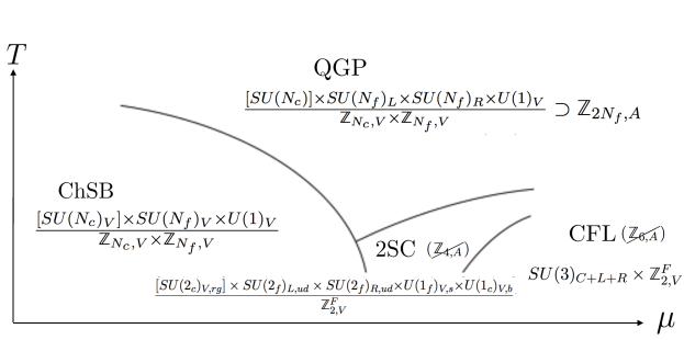
Figure 1: We revisit the QCD₄ matter phase in the $\mu$-T (chemical potential-temperature) phase diagram: The high T QGP (quark-gluon plasma/liquid), the low T ChSB (chiral symmetry breaking), 2SC (2-color superconductivity) and CFL (3-color-flavor locking superconductivity) at high density. We do not attempt to address the nature of phase transitions in this figure, thus we make some of the phase boundaries blur. The $\cancel{\mathbb{Z}_{6,A}}$ or $\cancel{\mathbb{Z}_{4,A}}$ means that part of the discrete axial symmetry $(A)$ is broken: $\cancel{\mathbb{Z}_{2N_{f},A}}$. In general, if the $G_{\text{sym}}$ group is broken, we denote it as $\cancel{G_{\text{sym}}}$.

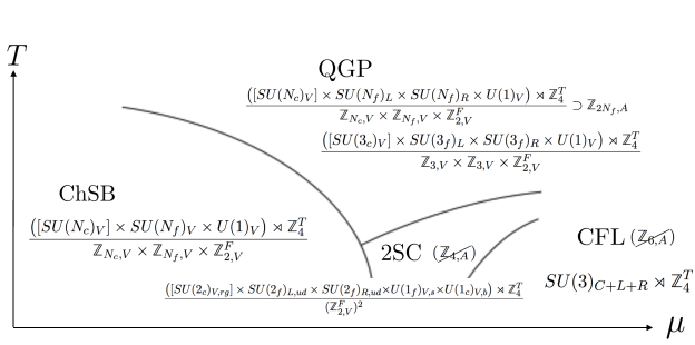
Figure 2: Follow Fig. 1, but now we include possible time-reversal symmetries, which can be any reasonable $\mathbb{Z}_{2}$-reflection symmetry by putting the Euclidean QCD₄ path integral on an unorientable spacetime. Here we choose a semi-direct product of $\rtimes\mathbb{Z}_{4}^{T}$, where $\mathbb{Z}_{4}^{T}\supset\mathbb{Z}_{2}^{F}$. The semi-direct product is more general, which also includes the direct product case of $\times\mathbb{Z}_{4}^{CT}$ as the $CT$ symmetry.

By including time reversal symmetries into the QCD system, we can choose any suitable outer automorphism of the color gauge or flavor global symmetry group as a $\mathbb{Z}_{2}$-time reversal symmetry, which is a $\mathbb{Z}_{2}$-reflection symmetry by putting the Euclidean QCD₄ path integral on an unorientable spacetime.

In fact, several recent works have attempted to study QCD matter phases based on the languages of higher symmetries and anomalies above. We should quickly overview some of these pioneer works:

1. Whether the color superconductivity can be topological in some way was questioned in LABEL:1001.2555Nishida. What LABEL:1001.2555Nishida concerns is the topological insulators (TI) / topological superconductors (TSC) in the free non-interacting quadratic mean-field Hamiltonian systems. Thus the classifications in LABEL:1001.2555Nishida are only either 0 or $\mathbb{Z}$ classes for mean-field free fermion systems. The new input in our context is that we consider fully interacting systems and enlist possible SPTs for these QCD matter phases by cobordism group classifications.

2. LABEL:Anber2018tcjPoppitz1805.12290,_Cordova2018acb1806.09592,_Bi2018xvrSenthil1808.07465,_Wan2018djlQCD1812.11955 explores a related system of 4d adjoint quantum chromodynamics (QCD₄) with an SU(2) gauge group and two massless adjoint Weyl fermions. Higher symmetries and higher anomalies play an important role. Depend on the complex mass parameters of fermions, we can land onto different phases, and there are interesting quantum phase transitions between bulk phases. There are implications and constraints for 3+1D deconfined quantum critical points (dQCP), quantum spin liquids (QSL) or fermionic liquids in condensed matter, and constraints on 3+1D ultraviolet-infrared (UV-IR) duality. See LABEL:Wan2018djlQCD1812.11955 for an overview of the proposed phases at quantum critical points.

3. LABEL:Bi2019ers1910.12856,_Wang2019obe1910.14664 explores quantum phase transitions between Landau ordering phase transitions but beyond the Landau paradigm, for example, due to the effects of topological $\theta$-terms. LABEL:Wang2019obe1910.14664 suggests that SU(2) QCD₄ with large odd number of flavors of quarks could be a direct second order phase transition between two phases of U(1) gauge theories as well as between a U(1) gauge theory and a trivial vacuum (e.g. a Landau symmetry-breaking gapped paramagnet). The gauge group is enhanced to be non-Abelian at and only at the transition. It is characterized as Gauge Enhanced Quantum Critical Points.

4. LABEL:1706.05385Unsal,_1706.06104Yonekura,_1711.10487Tanizaki,_Tanizaki2018wtg1807.07666,_Yonekura2019vyz1901.08188,_Anber2019nzeBCF1909.09027 employs global anomalies or global inconsistency of QCD₄ matter to constrain its QCD phase diagram, including either QCD zero-T phase or thermal phase. LABEL:1706.05385Unsal,_1706.06104Yonekura,_1711.10487Tanizaki,_Tanizaki2018wtg1807.07666,_Yonekura2019vyz1901.08188,_Anber2019nzeBCF1909.09027, implicitly or explicitly, suggests that there are obstructions or anomalies to simultaneously gauge or preserve both (1) a discrete axial symmetry and (2) a discrete 1-form color or flavor center symmetry (e.g. twisted discrete flavor-symmetry background boundary conditions or chemical potential $\mu$), and/or (3) under certain twisted boundary conditions — so preferably and naively either symmetries must be broken. In fact, there are still possibilities that symmetric gapped TQFTs can be constructed for some of these anomalies, for example, based on the symmetry extension method [43] or higher-symmetry extension method [34]. In any case, LABEL:1706.05385Unsal,_1706.06104Yonekura,_1711.10487Tanizaki,_Tanizaki2018wtg1807.07666,_Yonekura2019vyz1901.08188,_Anber2019nzeBCF1909.09027 can rule out trivial gapped phases under certain circumstances.

5. Quark-hadron continuity outside the Ginzburg-Landau paradigm: Quark-hadron continuity [44] asserts that hadronic matter superfluid phase is continuously connected to color-superconductor without phase transitions when the $\mu$ increases. This proposal is based on Ginzburg-Landau theory where two sides of phases have the similar symmetry breaking patterns and the similar gapless and gapped energetic spectrum. LABEL:Cherman2018jir1808.04827 questions the quark-hadron continuity to be invalid, by suggesting there must be a phase transition due to the topological fractionalization of excitations are different. LABEL:Hirono2018fjr1811.10608 re-analyzes the scenario based on higher-symmetry is not spontaneously broken, and found that the quark-hadron continuity is still plausible.

In the remained of this article, we like to point out a higher anomaly involving discrete 0-form axial chiral and 1-form mixed chiral-flavor-locked center symmetries that can be matched by the above four QCD phases. Then we will give a quick mathematical introduction of tools we used in Sec. 1.3. After then, we will list down various data and tables computed from cobordism theory, with a view toward the applications of QCD matter phases, to be studied in the future [47]. The QCD_d matter symmetries, anomalies, and topological terms without time-reversal symmetry, classified by the cobordism theory, are studied in Sec. 2 via a cobordism theory. The QCD_d matter symmetries, anomalies, and topological terms with time-reversal symmetry, classified by the cobordism theory, are studied in Sec. 3, in general in any spacetime dimensions $d=2,3,4,5$ via a cobordism theory.

1.2 Approximate higher anomaly constraint on the QCD phase diagram

In this section, we point out a higher ’t Hooft anomaly involving discrete 0-form axial and 1-form mixed chiral-flavor-locked center symmetries can be matched by the above four QCD phases. Our approach is related but still somehow different from LABEL:1706.05385Unsal,_1706.06104Yonekura,_1711.10487Tanizaki,_Tanizaki2018wtg1807.07666,_Yonekura2019vyz1901.08188,_Anber2019nzeBCF1909.09027.

For simplicity, we will set $N_{c}=N_{f}=N$ below. If $N_{c}\neq N_{f}$, we just need to replace the $N$ below to their greatest common divisor $\gcd(N_{c},N_{f})$ and make some moderate but a straightforward generalization.

First, under some assumptions that we will comment later, we hope to point out that there is an approximate 1-form electric-magnetic (e-m) global symmetry $\mathbb{Z}_{N_{cf},[1]}$ that mixed between 1-form color and flavor (CF) center symmetry: $\mathbb{Z}_{N_{cf},[1]}$. To recall, focus on the kinematics of the UV path integral of QFT,

($\bullet$1) If we do not have quarks in the fundamental Rep of the color gauge group $[{\rm SU}(N_{c})_{V}]$, then we have the 1-form electric symmetry $\mathbb{Z}_{N,c,[1]}$ whose charged objects are the color SU$(N_{c})$ fundamental Wilson line. If we have quarks in the fundamental Rep of $[{\rm SU}(N_{c})_{V}]$, then the $\mathbb{Z}_{N,c,[1]}$ is broken explicitly.

($\bullet$2) By looking at the largest symmetry at QCD phases — Eq. (1.3)’s QGP symmetry: $\frac{[{\rm SU}(N_{c})_{V}]\times{\rm SU}(N_{f})_{L}\times{\rm SU}(N_{f})_{R}\times{\rm U}(1)_{V}}{\mathbb{Z}_{N_{c},V}\times\mathbb{Z}_{N_{f},V}}$ where $[{\rm SU}(N_{c})_{V}]$ is gauged, we still are left with part of the projective special unitary symmetry $\frac{{\rm SU}(N_{f})_{V}}{\mathbb{Z}_{N_{f},V}}={\rm PSU}(N_{f})_{V}$ from the flavor symmetry. We can regarded it as a 1-form magnetic symmetry that can be coupled to the flavor symmetry background probed fields $\frac{{\rm SU}(N_{f})_{V}}{\mathbb{Z}_{N_{f},V}}={\rm PSU}(N_{f})_{V}$, by using the Stiefel-Whitney $w_{2}({\rm PSU}(N_{f})_{V})$. This idea is implemented already in [38, 39, 40, 41, 42].

($\bullet$3) Now we combine the above two 1-form e and m symmetries into a diagonal 1-form symmetry, and name it as 1-form electric-magnetic (e-m) global symmetry $\mathbb{Z}_{N_{cf},[1]}$. We define this 1-form e-m color-flavor-locked global symmetry $\mathbb{Z}_{N_{cf},[1]}$ as the diagonal symmetry that rotates oppositely the color-fundamental ($W_{c}$) and the flavor-fundamental ($W_{f}$) Wilson line along the 1d curve ${\gamma^{1}}$, called

$$W_{c}W_{f}=\exp(q_{c}\oint_{\gamma^{1}}a_{c})\exp(q_{f}\oint_{\gamma^{1}}a_{f}),$$ (1.7)

where the $a_{c}$ is. The $(W_{c}W_{f})$ have ends that can be opened by having bi-fundamental quark and anti-quark at each of two ends. Let us call the 2-dimensional surface operator that is the 1-form $\mathbb{Z}_{N_{cf},[1]}$ symmetry generator on 2d area ${\Sigma^{2}}$ as:

$$U\sim(U_{{\rm e},c})(U_{{\rm m},f})^{-1}\sim\exp(\oiint_{\Sigma^{2}}\Lambda)\exp(-\oiint_{\Sigma^{2}}w_{2}({\rm PSU}(N_{f})_{V})).$$ (1.8)

Here we write down the electric and magnetic 2-surface operators based on the conventions and notations in [16]. So that even if the bi-fundamental quarks can open up the the color-fundamental and the flavor-fundamental Wilson line, it will not be charged under the 1-form e-m $\mathbb{Z}_{N_{cf},[1]}$ symmetry, because the obtained phase is exactly cancelled:

$$\langle(U)(W_{c}W_{f})\rangle|_{\#_{U,(W_{c}W_{f}))}=1} = \exp(\hskip 1.0pt\mathrm{i}\hskip 1.0pt\frac{2\pi}{N})\exp(-\hskip 1.0pt\mathrm{i}\hskip 1.0pt\frac{2\pi}{N})\langle(U)(W_{c}W_{f})\rangle|_{\#_{U,(W_{c}W_{f}))}=0}$$ (1.9)

$$= 1\cdot\langle(U)(W_{c}W_{f})\rangle|_{\#_{U,(W_{c}W_{f}))}=0}$$

when the 2d $U$ surface and the 1d combined $W_{c}W_{f}$ line have a nontrivial linking number

$$\#_{U,(W_{c}W_{f}))}=1$$

in a 4d spacetime. Importantly, although bi-fundamental quarks can open up the $(W_{c}W_{f})$ line, physically this means that this (approximate) 1-form e-m $\mathbb{Z}_{N_{cf},[1]}$ symmetry is not broken (explicitly and kinematically) by the quark which must sit as bi-fundamental Rep in QCD₄!

However the 1-form e-m $\mathbb{Z}_{N_{cf},[1]}$ symmetry still acts nontrivially on the color-fundamental Wilson line because this linking

$$\langle(U)(W_{c})\rangle|_{\#_{U,(W_{c}W_{f}))}=1} = \exp(\hskip 1.0pt\mathrm{i}\hskip 1.0pt\frac{2\pi}{N})\langle(U)(W_{c})\rangle|_{\#_{U,(W_{c}W_{f}))}=0}$$ (1.10)

shows $W_{c}$ is charged under 1-form $\mathbb{Z}_{N_{cf},[1]}$ with a charge $\exp(\hskip 1.0pt\mathrm{i}\hskip 1.0pt\frac{2\pi}{N})$. Similarly, the 1-form e-m $\mathbb{Z}_{N_{cf},[1]}$ symmetry still acts nontrivially on the flavor-fundamental Wilson line because this linking

$$\langle(U)(W_{f})\rangle|_{\#_{U,(W_{c}W_{f}))}=1} = \exp(-\hskip 1.0pt\mathrm{i}\hskip 1.0pt\frac{2\pi}{N})\langle(U)(W_{f})\rangle|_{\#_{U,(W_{c}W_{f}))}=0}$$ (1.11)

shows $W_{f}$ is charged under 1-form $\mathbb{Z}_{N_{cf},[1]}$ symmetry with a charge $\exp(-\hskip 1.0pt\mathrm{i}\hskip 1.0pt\frac{2\pi}{N})$. We propose that there is an approximate anomaly mixing between the discrete $\mathbb{Z}_{2N_{f},A}$ axial (chiral) symmetry and the 1-form e-m color-flavor-locked ${\mathbb{Z}_{N_{cf},[1]}}$ global symmetry. We call the 2-form $\mathbb{Z}_{N}$ valued background field of 1-form $\mathbb{Z}_{N_{cf},[1]}$ as $B_{cf}^{(2)}$. We find that there is an anomaly captured by the $\mathbb{Z}_{2N_{f},A}$ axial (chiral) symmetry transformation, such that the partition function ${\mathbf{Z}}$ gains a fractionalized term

$${\mathbf{Z}}\xrightarrow[\text{}]{\mathbb{Z}_{2N_{f},A}\text{transformation}}{\mathbf{Z}}\cdot{\exp\big{(}\frac{{-\hskip 1.0pt\mathrm{i}\hskip 1.0ptN}}{2\pi}\int\limits_{M_{4}}(B_{cf}^{(2)}\wedge B_{cf}^{(2)})\big{)}}.$$ (1.12)

The fractionalized term ${\exp\big{(}\frac{{-\hskip 1.0pt\mathrm{i}\hskip 1.0ptN}}{2\pi}\int\limits_{M_{4}}(B_{cf}^{(2)}\wedge B_{cf}^{(2)})\big{)}}$ is not a 4d SPTs but a fractionalized 4d SPTs, not a counter term, thus cannot be absorbed into 4d, and should be regarded as a 5d higher-SPTs/higher-iTQFT – which in fact is an indicator of the 4d higher ’t Hooft anomaly of the QCD₄.

The caveat however is that this 4d higher ’t Hooft anomaly of the QCD₄ is only approximate. The subtlety is that it is only a precise anomaly if we also “gauge” the $\frac{{\rm SU}(N_{f})_{V}}{\mathbb{Z}_{N_{f},V}}={\rm PSU}(N_{f})_{V}$ sector into the $[\frac{{\rm SU}(N_{c})_{V}\times{\rm SU}(N_{f})_{V}}{\mathbb{Z}_{\gcd(N_{c},N_{f}),V}}]$ gauge theory. The disadvantages of our approximate anomaly (1.12) are that the flavor Wilson lines are only probed but not dynamical objects, so we do not really have the 1-form symmetry unless we at least weakly gauge the flavor symmetry. Thus another interpretation of our gauge theory and anomaly is indeed the bi-fundamental gauge theory in 3+1 dimensions studied in [50, 51].

In comparison, other approaches in LABEL:1706.05385Unsal,_1706.06104Yonekura,_1711.10487Tanizaki,_Tanizaki2018wtg1807.07666,_Yonekura2019vyz1901.08188,_Anber2019nzeBCF1909.09027 also have their own disadvantages. For example, LABEL:1711.10487Tanizaki derives a different kind of anomaly only under a certain twisted flavor boundary condition in 4d:

$${\mathbf{Z}}\xrightarrow[\text{}]{\mathbb{Z}_{2N_{f},A}\text{transformation}}{\mathbf{Z}}\cdot{\exp\big{(}\frac{{-\hskip 1.0pt\mathrm{i}\hskip 1.0ptN}}{2\pi}\int\limits_{M_{4}}(B_{c}^{(2)}\wedge B_{f}^{(2)})\big{)}}$$ (1.13)

and its dimensional reduction in 3d

$${\mathbf{Z}}\xrightarrow[\text{}]{\mathbb{Z}_{2N_{f},A}\text{transformation}}{\mathbf{Z}}\cdot{\exp\big{(}\frac{{-\hskip 1.0pt\mathrm{i}\hskip 1.0ptN}}{2\pi}\int\limits_{M_{4}}(B_{c}^{(1)}\wedge B_{f}^{(2)})\big{)}},$$ (1.14)

where $B_{c}$ and $B_{f}$ are color/flavor background fields respectively. LABEL:1706.06104Yonekura derives constraints that have limitations on the chemical potential and boundary conditions as well.

In Figure 3, we show how our approximate anomaly in (1.12) is still required and can be matched by the four QCD₄ matter phases.

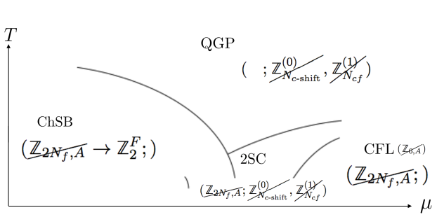
Figure 3: Follow Fig. 1 and Fig. 2, QCD₄ matter phases shown here include the high T QGP (quark-gluon plasma/liquid), the low T ChSB (chiral symmetry breaking), 2SC (2-color superconductivity) and CFL (3-color-flavor locking superconductivity) at high density. The four phases can be matched and cancelled by our approximate anomaly (1.12), ${\mathbf{Z}}\xrightarrow[\text{}]{\mathbb{Z}_{2N_{f},A}\text{transformation}}{\mathbf{Z}}\cdot{\exp\big{(}\frac{{-\hskip 1.0pt\mathrm{i}\hskip 1.0ptN}}{2\pi}\int\limits_{M_{4}}(B_{cf}^{(2)}\wedge B_{cf}^{(2)})\big{)}}$. The four phases can also be matched and cancelled by the anomaly (1.14), ${\mathbf{Z}}\xrightarrow[\text{}]{\mathbb{Z}_{2N_{f},A}\text{transformation}}{\mathbf{Z}}\cdot{\exp\big{(}\frac{{-\hskip 1.0pt\mathrm{i}\hskip 1.0ptN}}{2\pi}\int\limits_{M_{4}}(B_{c}^{(1)}\wedge B_{f}^{(2)})\big{)}}$ introduced in LABEL:1706.06104Yonekura. We use the triple data $(\mathbb{Z}_{2N_{f},A};\mathbb{Z}_{N_{c\text{-shift}}}^{(0)},{\mathbb{Z}^{{(1)}}_{N_{cf}}})$ to label the discrete 0-form axial symmetry $\mathbb{Z}_{2N_{f},A}$, a dimensionally reduced color-shift $\mathbb{Z}_{N_{c\text{-shift}}}^{(0)}$ symmetry introduced in LABEL:1706.06104Yonekura , and the 1-form mixed chiral-flavor-locked center symmetry ${\mathbb{Z}^{{(1)}}_{N_{cf}}}$ that we introduce.

We use the triple data with three imputs

$$(\mathbb{Z}_{2N_{f},A};\mathbb{Z}_{N_{c\text{-shift}}},{\mathbb{Z}_{N_{cf},[1]}})$$ (1.15)

which in Fig. 3 can be also denoted as

$$(\mathbb{Z}_{2N_{f},A};\mathbb{Z}_{N_{c\text{-shift}}}^{(0)},{\mathbb{Z}^{{(1)}}_{N_{cf}}}),$$ (1.16)

where the upper index ${{(1)}}$ in ${\mathbb{Z}^{{(1)}}_{N_{cf}}}$ indicates it is truly a 1-form symmetry in (1.12), while the upper index ${{(0)}}$ in $\mathbb{Z}_{N_{c\text{-shift}}}^{(0)}$ indicates it is dimensionally reduced from 1-form symmetry $\mathbb{Z}_{N_{c\text{-shift}},[1]}$ to a 0-form symmetry. The 1-form color-shift symmetry $\mathbb{Z}_{N_{c\text{-shift}},[1]}$ is introduced in LABEL:1706.06104Yonekura.

Let us indicate how the higher ’t Hooft anomalies in (1.12) and in (1.14) can be matched by breaking some of the global symmetries in the triple data $(\mathbb{Z}_{2N_{f},A};{\mathbb{Z}^{{(1)}}_{N_{cf}}},\mathbb{Z}_{N_{c\text{-shift}}}^{(0)})$. Our notations are that if the $G_{\text{sym}}$ is broken, we denote it as $\cancel{G_{\text{sym}}}$, if the $G_{\text{sym}}$ is preserved, we would either indicate $G_{\text{sym}}$ remained, or simply omit the symbol as we did in the Fig. 3.

1. QGP (quark-gluon plasma/liquid) at high T:

   $$(\mathbb{Z}_{2N_{f},A};\mathbb{Z}_{N_{c\text{-shift}}}^{(0)},{\mathbb{Z}^{{(1)}}_{N_{cf}}})\xrightarrow[]{\text{SSB}}(\mathbb{Z}_{2N_{f},A};\cancel{\mathbb{Z}_{N_{c\text{-shift}}}^{(0)}},\cancel{\mathbb{Z}^{{(1)}}_{N_{cf}}})\sim(\quad;\cancel{\mathbb{Z}_{N_{c\text{-shift}}}^{(0)}},\cancel{\mathbb{Z}^{{(1)}}_{N_{cf}}})\text{ shown in Fig.~{}\ref{fig:qcd-phase-break} QGP}.$$ (1.17)

2. ChSB (chiral symmetry breaking) at low T and at lower densities and low $\mu$:

   $$(\mathbb{Z}_{2N_{f},A};\mathbb{Z}_{N_{c\text{-shift}}}^{(0)},{\mathbb{Z}^{{(1)}}_{N_{cf}}})\xrightarrow[]{\text{SSB}}(\cancel{\mathbb{Z}_{2N_{f},A}}\to\mathbb{Z}_{2}^{F};\mathbb{Z}_{N_{c\text{-shift}}}^{(0)},{\mathbb{Z}^{{(1)}}_{N_{cf}}})\sim(\cancel{\mathbb{Z}_{2N_{f},A}}\to\mathbb{Z}_{2}^{F};)\text{ shown in Fig.~{}\ref{fig:qcd-phase-break} ChSB}.\quad$$ (1.18)

3. 2SC (2-color superconductivity) at low T and at intermediate densities and $\mu$:

   $$(\mathbb{Z}_{2N_{f},A};\mathbb{Z}_{N_{c\text{-shift}}}^{(0)},{\mathbb{Z}^{{(1)}}_{N_{cf}}})\xrightarrow[]{\text{SSB}}(\cancel{\mathbb{Z}_{2N_{f},A}};\cancel{\mathbb{Z}_{N_{c\text{-shift}}}^{(0)}},\cancel{\mathbb{Z}^{{(1)}}_{N_{cf}}})\text{ shown in Fig.~{}\ref{fig:qcd-phase-break} 2SC}.\quad$$ (1.19)

4. CFL (3-color-flavor locking superconductivity) at low T and at high density and high $\mu$:

   $$(\mathbb{Z}_{2N_{f},A};\mathbb{Z}_{N_{c\text{-shift}}}^{(0)},{\mathbb{Z}^{{(1)}}_{N_{cf}}})\xrightarrow[]{\text{SSB}}(\cancel{\mathbb{Z}_{2N_{f},A}};{\mathbb{Z}_{N_{c\text{-shift}}}^{(0)}},{\mathbb{Z}^{{(1)}}_{N_{cf}}})\sim(\cancel{\mathbb{Z}_{2N_{f},A}};)\text{ shown in Fig.~{}\ref{fig:qcd-phase-break} CFL}.\quad$$ (1.20)

What we have shown above is that higher ’t Hooft anomalies in (1.12) and in (1.14) can indeed be matched by four phases via breaking some of the global symmetries. We thus can constrain other possible QCD phases via the proposed approximate anomaly (1.12), based on higher ’t Hooft anomaly matching and cancellation.

1.3 Mathematical Primer

In this article, we use spectral sequences (Adams spectral sequence, Atiyah-Hirzebruch spectral sequence, and Serre spectral sequence) to compute several cobordism groups which appear in QCD matter phases (QGP, ChSB, 2SC and CFL in Sec. 1.1). See [4, 29, 52] for a primer.

We aim to compute the cobordism group $\Omega_{d}^{G}$ for $d\leq 5$ where $G$ is the gauge group of QCD matter phases (QGP, ChSB, 2SC and CFL).

By the generalized Pontryagin-Thom isomorphism,

$$\Omega_{d}^{G}=\pi_{d}(MTG)$$ (1.21)

which identifies the cobordism group $\Omega_{d}^{G}$ with the homotopy group of the Madsen-Tillmann spectrum $MTG$.

We have the Adams spectral sequence

$$\operatorname{Ext}_{\mathcal{A}_{p}}^{s,t}(\operatorname{H}^{*}(Y,\mathbb{Z}_{p}),\mathbb{Z}_{p})\Rightarrow\pi_{t-s}(Y)_{p}^{\wedge}.$$ (1.22)

Here $\mathcal{A}_{p}$ is the mod $p$ Steenrod algebra, $Y$ is any spectrum. For any finitely generated abelian group $G$, $G_{p}^{\wedge}=\lim_{n\to\infty}G/p^{n}G$ is the $p$-completion of $G$. In particular, $\mathcal{A}_{2}$ is generated by Steenrod squares $\mathrm{Sq}^{i}$.

In our cases, the cobordism groups only have 2-torsion and 3-torsion.

We will use Adams spectral sequence to compute the 2-torsion part of the cobordism groups (we consider $Y=MTG$ in Adams spectral sequence, and we focus on $p=2$).

We will use Serre spectral sequence and Atiyah-Hirzebruch spectral sequence to compute the 3-torsion part of the cobordism groups. In our cases, in order to compute the 3-torsion part of the cobordism groups, we need only to compute the cobordism group $\Omega_{d}^{{\rm SO}}(\mathrm{B}G^{\prime})$ for some group $G^{\prime}$.

We have the Atiyah-Hirzebruch spectral sequence

$$\operatorname{H}_{p}(\mathrm{B}G^{\prime},\Omega_{q}^{{\rm SO}})\Rightarrow\Omega_{p+q}^{{\rm SO}}(\mathrm{B}G^{\prime}).$$ (1.23)

Since

$$\Omega_{d}^{{\rm SO}}=\left\{\begin{array}[]{ll}\mathbb{Z}&d=0\\ 0&d=1\\ 0&d=2\\ 0&d=3\\ \mathbb{Z}&d=4\\ \mathbb{Z}_{2}&d=5\end{array}\right.,$$ (1.30)

we need to know the integral homology groups $\operatorname{H}_{p}(\mathrm{B}G^{\prime},\mathbb{Z})$. In order to obtain this data, we compute the integral cohomology groups $\operatorname{H}^{p}(\mathrm{B}G^{\prime},\mathbb{Z})$ using Serre spectral sequence (we find a fibration of which $\mathrm{B}G^{\prime}$ is the total space).

For example, if $MTG=M{\rm Spin}\wedge X$ where $X$ is any spectrum, by Corollary 5.1.2 of [53], we have

$$\operatorname{Ext}_{\mathcal{A}_{2}}^{s,t}(\operatorname{H}^{*}(M{\rm Spin}\wedge X,\mathbb{Z}_{2}),\mathbb{Z}_{2})=\operatorname{Ext}_{\mathcal{A}_{2}(1)}^{s,t}(\operatorname{H}^{*}(X,\mathbb{Z}_{2}),\mathbb{Z}_{2})$$ (1.31)

for $t-s<8$. Here $\mathcal{A}_{2}(1)$ is the subalgebra of $\mathcal{A}_{2}$ generated by $\mathrm{Sq}^{1}$ and $\mathrm{Sq}^{2}$.

So for the dimension $d=t-s<8$, we have

$$\operatorname{Ext}_{\mathcal{A}_{2}(1)}^{s,t}(\operatorname{H}^{*}(X,\mathbb{Z}_{2}),\mathbb{Z}_{2})\Rightarrow(\Omega_{t-s}^{G})_{2}^{\wedge}.$$ (1.32)

The $\operatorname{H}^{*}(X,\mathbb{Z}_{2})$ is an $\mathcal{A}_{2}(1)$-module whose internal degree $t$ is given by the $*$.

Our computation of $E_{2}$ pages of $\mathcal{A}_{2}(1)$-modules is based on Lemma 11 of [29]. More precisely, we find a short exact sequence of $\mathcal{A}_{2}(1)$-modules $0\to L_{1}\to L_{2}\to L_{3}\to 0$, then apply Lemma 11 of [29] to compute $\operatorname{Ext}_{\mathcal{A}_{2}(1)}^{s,t}(L_{2},\mathbb{Z}_{2})$ by the data of $\operatorname{Ext}_{\mathcal{A}_{2}(1)}^{s,t}(L_{1},\mathbb{Z}_{2})$ and $\operatorname{Ext}_{\mathcal{A}_{2}(1)}^{s,t}(L_{3},\mathbb{Z}_{2})$. Our strategy is choosing $L_{1}$ to be the direct sum of suspensions of $\mathbb{Z}_{2}$ on which $\mathrm{Sq}^{1}$ and $\mathrm{Sq}^{2}$ act trivially, then we take $L_{3}$ to be the quotient of $L_{2}$ by $L_{1}$. We can use this procedure again and again until $\operatorname{Ext}_{\mathcal{A}_{2}(1)}^{s,t}(L_{3},\mathbb{Z}_{2})$ is determined.

2 QCD Symmetries, Anomalies and Topological Terms Without Time-Reversal

Before we consider the cobordism theory and co/bordism group of the following four QCD matter phases, we need to convert our notations to involve both the internal symmetry and the spacetime symmetry. Here are the results of conversions for the high T QGP (quark-gluon plasma/liquid), the low T ChSB (chiral symmetry breaking), 2SC (2-color superconductivity) and CFL (3-color-flavor locking superconductivity) at high density.
QGP:

$$\frac{[{\rm SU}(N_{c})_{V}]\times{\rm SU}(N_{f})_{L}\times{\rm SU}(N_{f})_{R}\times{\rm U}(1)_{V}}{\mathbb{Z}_{N_{c},V}\times\mathbb{Z}_{N_{f},V}}:=\Big{(}{\rm Spin}(d)\times_{\mathbb{Z}_{2}}\frac{{\rm SU}(3)_{L}\times{\rm SU}(3)_{R}\times{\rm U}(1)_{V}}{(\mathbb{Z}_{3})^{2}}\Big{)}$$

$$=\Big{(}{\rm Spin}(d)\times_{\mathbb{Z}_{2}}\frac{{\rm U}(3)_{L}\times{\rm U}(3)_{R}}{(\mathbb{Z}_{3})^{2}\times{\rm U}(1)_{A}}\Big{)}\times\mathbb{Z}_{3,L}\times\mathbb{Z}_{3,R}=\Big{(}{\rm Spin}(d)\times_{\mathbb{Z}_{2}}\frac{{\rm U}(3)_{L}\times{\rm U}(3)_{R}}{(\mathbb{Z}_{3,V}\times\mathbb{Z}_{3,A}\times{\rm U}(1)_{A})}\Big{)}.$$ (2.1)

Here ${\rm U}(1)_{V}=\frac{{\rm U}(1)_{L}\times{\rm U}(1)_{R}}{{\rm U}(1)_{A}}$, ${\rm U}(3)_{L}=\frac{{\rm SU}(3)_{L}\times{\rm U}(1)_{L}}{\mathbb{Z}_{3,L}}$, ${\rm U}(3)_{R}=\frac{{\rm SU}(3)_{R}\times{\rm U}(1)_{R}}{\mathbb{Z}_{3,R}}$ where $L/R$ for $P_{L/R}=\frac{1\pm\gamma^{5}}{2}$ ChSB:

$${\frac{\big{(}[{\rm SU}(N_{c})_{V}]\times{\rm SU}(N_{f})_{V}\times{\rm U}(1)_{V}\big{)}}{\mathbb{Z}_{N_{c},V}\times\mathbb{Z}_{N_{f},V}}}:=\Big{(}{\rm Spin}(d)\times_{\mathbb{Z}_{2}}\frac{{\rm SU}(3)\times{\rm U}(1)}{(\mathbb{Z}_{3})^{2}}\Big{)}=\Big{(}{\rm Spin}(d)\times_{\mathbb{Z}_{2}}\frac{{\rm U}(3)}{\mathbb{Z}_{3}}\Big{)}.$$ (2.2)

2SC:

$$\frac{[{\rm SU}(2_{c})_{V,rg}]\times{\rm SU}(2_{f})_{L,ud}\times{\rm SU}(2_{f})_{R,ud}{\times{\rm U}(1_{f})_{V,s}}{\times{\rm U}(1_{c})_{V,b}}}{{\mathbb{Z}_{2,V}^{F}}}:=\Big{(}{\rm Spin}(d)\times_{\mathbb{Z}_{2}}({\rm SU}(2)\times{\rm SU}(2))\Big{)}\times({\rm U}(1)\times{\rm U}(1)).$$ (2.3)

CFL:

$${\rm SU}(3)_{C+L+R}\times\mathbb{Z}_{2,V}^{F}:={\rm Spin}(d)\times{\rm SU}(3)_{C+L+R}.$$ (2.4)

2.1 Chiral symmetry breaking ${\frac{\big{(}[{\rm SU}(3)_{V}]\times{\rm SU}(3)_{V}\times{\rm U}(1)_{V}\big{)}}{\mathbb{Z}_{3_{c},V}\times\mathbb{Z}_{3_{f},V}}}$ as $({\rm Spin}(d)\times_{\mathbb{Z}_{2}}\frac{{\rm U}(3)}{\mathbb{Z}_{3}})$

For ChSB with a global symmetry:

$${\frac{\big{(}[{\rm SU}(N_{c})_{V}]\times{\rm SU}(N_{f})_{V}\times{\rm U}(1)_{V}\big{)}}{\mathbb{Z}_{N_{c},V}\times\mathbb{Z}_{N_{f},V}}}:=\Big{(}{\rm Spin}(d)\times_{\mathbb{Z}_{2}}\frac{{\rm SU}(3)\times{\rm U}(1)}{(\mathbb{Z}_{3})^{2}}\Big{)}=\Big{(}{\rm Spin}(d)\times_{\mathbb{Z}_{2}}\frac{{\rm U}(3)}{\mathbb{Z}_{3}}\Big{)}.$$

We have a fibration

(2.9)

Hence we have the Serre spectral sequence, see Figure 4.

$$\operatorname{H}^{p}(\mathrm{B}^{2}\mathbb{Z}_{3},\operatorname{H}^{q}(\mathrm{B}{\rm U}(3),\mathbb{Z}))\Rightarrow\operatorname{H}^{p+q}(\mathrm{B}(\frac{{\rm U}(3)}{\mathbb{Z}_{3}}),\mathbb{Z}).$$ (2.10)

We have

$$\operatorname{H}^{*}(\mathrm{B}{\rm U}(3),\mathbb{Z})=\mathbb{Z}[c_{1},c_{2},c_{3}]$$ (2.11)

and

$$\operatorname{H}^{p}(\mathrm{B}^{2}\mathbb{Z}_{3},\mathbb{Z})=\left\{\begin{array}[]{llllllll}\mathbb{Z}&p=0\\ 0&p=1\\ 0&p=2\\ \mathbb{Z}_{3}&p=3\\ 0&p=4\\ \mathbb{Z}_{3}&p=5\\ 0&p=6\\ \mathbb{Z}_{9}&p=7\end{array}\right..$$ (2.20)

[grid=none,labelstep=1,entrysize=1.5cm]0…70…6 Z 1 0 0 2 0 0 3 0 Z_3 4 0 0 5 0 Z_3 6 0 0 7 0 Z_9 0 1 0 1 1 0 2 1 0 3 1 0 4 1 0 5 1 0 6 1 0 7 1 0 0 2 Z 1 2 0 2 2 0 3 2 Z_3 4 2 0 5 2 Z_3 6 2 0 7 2 Z_9 0 3 0 1 3 0 2 3 0 3 3 0 4 3 0 5 3 0 6 3 0 7 3 0 0 4 Z^2 1 4 0 2 4 0 3 4 Z_3^2 4 4 0 5 4 Z_3^2 6 4 0 7 4 Z_9^2 0 5 0 1 5 0 2 5 0 3 5 0 4 5 0 5 5 0 6 5 0 7 5 0 0 6 Z^3 1 6 0 2 6 0 3 6 Z_3^3 4 6 0 5 6 Z_3^3 6 6 0 7 6 Z_9^3

0 4 [color=red] 5 -4

0 4 [color=red,dashed] 3 -2

Figure 4: Serre spectral sequence for the fibration $\mathrm{B}{\rm U}(3)\to\mathrm{B}(\frac{{\rm U}(3)}{\mathbb{Z}_{3}})\to\mathrm{B}^{2}\mathbb{Z}_{3}$. The arrow from (0,4) to (5,0) is a nontrivial differential by comparison with the Serre spectral sequence of the fibration $\mathrm{B}{\rm SU}(3)\to\mathrm{B}{\rm PSU}(3)\to\mathrm{B}^{2}\mathbb{Z}_{3}$. There is no differential from (0,2) to (3,0) since the 3d $\mathbb{Z}_{3}$ survives the spectral sequence in Figure 5.

There is another approach: we have a fibration

(2.25)

Hence we have the Serre spectral sequence, see Figure 5.

$$\operatorname{H}^{p}(\mathrm{B}{\rm U}(1),\operatorname{H}^{q}(\mathrm{B}{\rm PSU}(3),\mathbb{Z}))\Rightarrow\operatorname{H}^{p+q}(\mathrm{B}(\frac{{\rm U}(3)}{\mathbb{Z}_{3}}),\mathbb{Z}).$$ (2.26)

We have

$$\operatorname{H}^{*}(\mathrm{B}{\rm U}(1),\mathbb{Z})=\mathbb{Z}[c_{1}]$$ (2.27)

and

$$\operatorname{H}^{p}(\mathrm{B}{\rm PSU}(3),\mathbb{Z})=\left\{\begin{array}[]{llllllll}\mathbb{Z}&p=0\\ 0&p=1\\ 0&p=2\\ \mathbb{Z}_{3}&p=3\\ \mathbb{Z}&p=4\\ 0&p=5\\ \mathbb{Z}&p=6\end{array}\right..$$ (2.35)

[grid=none,labelstep=1,entrysize=1.5cm]0…60…6 Z 1 0 0 2 0 Z 3 0 0 4 0 Z 5 0 0 6 0 Z

0 1 0 1 1 0 2 1 0 3 1 0 4 1 0 5 1 0 6 1 0

0 2 0 1 2 0 2 2 0 3 2 0 4 2 0 5 2 0 6 2 0

0 3 Z_3 1 3 0 2 3 Z_3 3 3 0 4 3 Z_3 5 3 0 6 3 Z_3

0 4 Z 1 4 0 2 4 Z 3 4 0 4 4 Z 5 4 0 6 4 Z

0 5 0 1 5 0 2 5 0 3 5 0 4 5 0 5 5 0 6 5 0

0 6 Z 1 6 0 2 6 Z 3 6 0 4 6 Z 5 6 0 6 6 Z

0 4 [color=red,dashed] 2 -1

Figure 5: Serre spectral sequence for the fibration $\mathrm{B}{\rm PSU}(3)\to\mathrm{B}(\frac{{\rm U}(3)}{\mathbb{Z}_{3}})\to\mathrm{B}{\rm U}(1)$.

In Figure 5, we find that the 3d $\mathbb{Z}_{3}$ survives the spectral sequence, so in Figure 4, there is no nontrivial differential from (0,2) to (3,0). Since the differential is a derivation, we conclude that in Figure 4 the dashed arrow from (0,4) to (3,2) does not actually exist. So there is a $\mathbb{Z}_{3}$ in 5d survives the spectral sequence, thus in Figure 5, the dashed arrow from (0,4) to (2,3) also does not actually exist.

So

$$\operatorname{H}^{p}(\mathrm{B}(\frac{{\rm U}(3)}{\mathbb{Z}_{3}}),\mathbb{Z})=\left\{\begin{array}[]{lllllll}\mathbb{Z}&p=0\\ 0&p=1\\ \mathbb{Z}&p=2\\ \mathbb{Z}_{3}&p=3\\ \mathbb{Z}^{2}&p=4\\ \mathbb{Z}_{3}&p=5\\ \mathbb{Z}^{3}&p=6\end{array}\right.$$ (2.43)

and

$$\operatorname{H}_{p}(\mathrm{B}(\frac{{\rm U}(3)}{\mathbb{Z}_{3}}),\mathbb{Z})=\left\{\begin{array}[]{lllllll}\mathbb{Z}&p=0\\ 0&p=1\\ \mathbb{Z}\times\mathbb{Z}_{3}&p=2\\ 0&p=3\\ \mathbb{Z}^{2}\times\mathbb{Z}_{3}&p=4\\ 0&p=5\\ \mathbb{Z}^{3}\times?&p=6\end{array}\right..$$ (2.51)

Here ? is an undetermined 3-torsion group.

By the Atiyah-Hirzebruch spectral sequence, we have

$$\operatorname{H}_{p}(\mathrm{B}(\frac{{\rm U}(3)}{\mathbb{Z}_{3}}),\Omega_{q}^{{\rm SO}})\Rightarrow\Omega_{p+q}^{{\rm SO}}(\mathrm{B}(\frac{{\rm U}(3)}{\mathbb{Z}_{3}})).$$ (2.52)

See Figure 6.

[grid=none,labelstep=1,entrysize=1.5cm]0…60…5 Z 1 0 0 2 0 Z×Z_3 3 0 0 4 0 Z^2×Z_3 5 0 0 6 0 Z^3×? 0 1 0 1 1 0 2 1 0 3 1 0 4 1 0 5 1 0

0 2 0 1 2 0 2 2 0 3 2 0 4 2 0

0 3 0 1 3 0 2 3 0 3 3 0 0 4 Z 1 4 0 2 4 Z×Z_3 0 5 Z_2

Figure 6: Atiyah-Hirzebruch spectral sequence for $\Omega_{d}^{{\rm SO}\times\frac{{\rm U}(3)}{\mathbb{Z}_{3}}}$. Here ? is an undetermined 3-torsion group.

Since the localization of ${\rm Spin}\times_{\mathbb{Z}_{2}}\frac{{\rm U}(3)}{\mathbb{Z}_{3}}$ and ${\rm SO}\times\frac{{\rm U}(3)}{\mathbb{Z}_{3}}$ at the prime 3 are the same, the 3-torsion part of $\Omega_{d}^{{\rm Spin}\times_{\mathbb{Z}_{2}}\frac{{\rm U}(3)}{\mathbb{Z}_{3}}}$ and $\Omega_{d}^{{\rm SO}\times\frac{{\rm U}(3)}{\mathbb{Z}_{3}}}$ are the same.

Since the localization of ${\rm Spin}\times_{\mathbb{Z}_{2}}\frac{{\rm U}(3)}{\mathbb{Z}_{3}}$ and ${\rm Spin}\times_{\mathbb{Z}_{2}}{\rm U}(3)$ at the prime 2 are the same, the 2-torsion part of $\Omega_{d}^{{\rm Spin}\times_{\mathbb{Z}_{2}}\frac{{\rm U}(3)}{\mathbb{Z}_{3}}}$ and $\Omega_{d}^{{\rm Spin}\times_{\mathbb{Z}_{2}}{\rm U}(3)}$ are the same.

Also since ${\rm U}(3)={\rm SU}(3)\times_{\mathbb{Z}_{3}}{\rm U}(1)$, the localization of ${\rm Spin}\times_{\mathbb{Z}_{2}}{\rm U}(3)$ and ${\rm Spin}\times_{\mathbb{Z}_{2}}({\rm U}(1)\times{\rm SU}(3))$ at the prime 2 are the same, the 2-torsion part of $\Omega_{d}^{{\rm Spin}\times_{\mathbb{Z}_{2}}{\rm U}(3)}$ and $\Omega_{d}^{{\rm Spin}\times_{\mathbb{Z}_{2}}({\rm U}(1)\times{\rm SU}(3))}=\Omega_{d}^{{\rm Spin}^{c}\times{\rm SU}(3)}$ are the same.

We have $MT({\rm Spin}^{c}\times{\rm SU}(3))=M{\rm Spin}\wedge\Sigma^{-2}M{\rm U}(1)\wedge(\mathrm{B}{\rm SU}(3))_{+}$.

For $t-s<8$, since there is no odd torsion, we have the Adams spectral sequence

$$\operatorname{Ext}_{\mathcal{A}_{2}(1)}^{s,t}(\operatorname{H}^{*+2}(M{\rm U}(1),\mathbb{Z}_{2})\otimes\operatorname{H}^{*}(\mathrm{B}{\rm SU}(3),\mathbb{Z}_{2}),\mathbb{Z}_{2})\Rightarrow\Omega_{t-s}^{{\rm Spin}^{c}\times{\rm SU}(3)}.$$ (2.53)

We have

$$\operatorname{H}^{*}(\mathrm{B}{\rm SU}(3),\mathbb{Z}_{2})=\mathbb{Z}_{2}[c_{2},c_{3}]$$ (2.54)

where $c_{i}$ is the Chern class of the ${\rm SU}(3)$ bundle.

By Thom isomorphism,

$$\operatorname{H}^{*+2}(M{\rm U}(1),\mathbb{Z}_{2})=\mathbb{Z}_{2}[c_{1}]U$$ (2.55)

where $c_{1}$ is the Chern class of the ${\rm U}(1)$ bundle and $U$ is the Thom class.

The $\mathcal{A}_{2}(1)$-module structure of $\operatorname{H}^{*+2}(M{\rm U}(1),\mathbb{Z}_{2})\otimes\operatorname{H}^{*}(\mathrm{B}{\rm SU}(3),\mathbb{Z}_{2})$ below degree 6 and the $E_{2}$ page are shown in Figure 7, 8.

Figure 7: The $\mathcal{A}_{2}(1)$-module structure of $\operatorname{H}^{*+2}(M{\rm U}(1),\mathbb{Z}_{2})\otimes\operatorname{H}^{*}(\mathrm{B}{\rm SU}(3),\mathbb{Z}_{2})$ below degree 6.

Figure 8: $\Omega_{*}^{{\rm Spin}^{c}\times{\rm SU}(3)}$.

So there is no 2-torsion in $\Omega^{{\rm Spin}\times_{\mathbb{Z}_{2}}\frac{{\rm U}(3)}{\mathbb{Z}_{3}}}_{d}$.

Combine the 2-torsion and 3-torsion results, we have

Bordism group
$d$	$\Omega^{{\rm Spin}\times_{\mathbb{Z}_{2}}\frac{{\rm U}(3)}{\mathbb{Z}_{3}}}_{d}$	generators
0	$\mathbb{Z}$
1	0
2	$\mathbb{Z}\times\mathbb{Z}_{3}$
3	$0$
4	$e(\mathbb{Z}^{2}\times\mathbb{Z}_{3},\mathbb{Z})$
5	$0$

Table 3: Bordism group. The notation $e(A,B)$ denotes a group extension of A by B, that is, a group that fits into the following short exact sequence $0\to B\to e(A,B)\to A\to 0$.

2.2 3-Color-Flavor locking superconductivity ${\rm SU}(3)_{C+L+R}\times\mathbb{Z}_{2,V}^{F}$ as ${\rm Spin}\times{\rm SU}(3)$

We have $MT({\rm Spin}\times{\rm SU}(3))=M{\rm Spin}\wedge(\mathrm{B}{\rm SU}(3))_{+}$.

For $t-s<8$, since there is no odd torsion, we have the Adams spectral sequence

$$\operatorname{Ext}_{\mathcal{A}_{2}(1)}^{s,t}(\operatorname{H}^{*}(\mathrm{B}{\rm SU}(3),\mathbb{Z}_{2}),\mathbb{Z}_{2})\Rightarrow\Omega_{t-s}^{{\rm Spin}\times{\rm SU}(3)}.$$ (2.56)

We have

$$\operatorname{H}^{*}(\mathrm{B}{\rm SU}(3),\mathbb{Z}_{2})=\mathbb{Z}_{2}[c_{2},c_{3}]$$ (2.57)

where $c_{i}$ is the Chern class of the ${\rm SU}(3)$ bundle.

The $\mathcal{A}_{2}(1)$-module structure of $\operatorname{H}^{*}(\mathrm{B}{\rm SU}(3),\mathbb{Z}_{2})$ below degree 6 and the $E_{2}$ page are shown in Figure 9, 10.

Figure 9: The $\mathcal{A}_{2}(1)$-module structure of $\operatorname{H}^{*}(\mathrm{B}{\rm SU}(3),\mathbb{Z}_{2})$ below degree 6.

Figure 10: $\Omega_{*}^{{\rm Spin}\times{\rm SU}(3)}$.

Bordism group
$d$	$\Omega^{{\rm Spin}\times{\rm SU}(3)}_{d}$	generators
0	$\mathbb{Z}$
1	$\mathbb{Z}_{2}$	$\tilde{\eta}$
2	$\mathbb{Z}_{2}$	Arf
3	$0$
4	$\mathbb{Z}^{2}$	$\frac{\sigma}{16},c_{2}$
5	$0$
6	$\mathbb{Z}$	$\frac{c_{3}}{2}$

Table 4: Bordism group. $\tilde{\eta}$ is a mod 2 index of 1d Dirac operator. Arf is a 2d Arf invariant. $\sigma$ is the signature of manifold. Note that $c_{3}=\mathrm{Sq}^{2}c_{2}=(w_{2}+w_{1}^{2})c_{2}=0\mod 2$ on Spin 6-manifolds.

2.3 2-Color Superconductivity: $\frac{[{\rm SU}(2_{c})_{V,rg}]\times{\rm SU}(2_{f})_{L,ud}\times{\rm SU}(2_{f})_{R,ud}{\times{\rm U}(1_{f})_{V,s}}{\times{\rm U}(1_{c})_{V,b}}}{{\mathbb{Z}_{2,V}^{F}}}$ as ${\rm Spin}\times_{\mathbb{Z}_{2}}{\rm Spin}(4)\times{\rm U}(1)\times{\rm U}(1)$

We have $MT({\rm Spin}\times_{\mathbb{Z}_{2}}{\rm Spin}(4)\times{\rm U}(1)\times{\rm U}(1))=M{\rm Spin}\wedge\Sigma^{-4}M{\rm SO}(4)\wedge(\mathrm{B}{\rm U}(1)\times\mathrm{B}{\rm U}(1))_{+}$.

For $t-s<8$, since there is no odd torsion, we have the Adams spectral sequence

$$\operatorname{Ext}_{\mathcal{A}_{2}(1)}^{s,t}(\operatorname{H}^{*+4}(M{\rm SO}(4),\mathbb{Z}_{2})\otimes\operatorname{H}^{*}(\mathrm{B}{\rm U}(1),\mathbb{Z}_{2})\otimes\operatorname{H}^{*}(\mathrm{B}{\rm U}(1),\mathbb{Z}_{2}),\mathbb{Z}_{2})\Rightarrow\Omega_{t-s}^{{\rm Spin}\times_{\mathbb{Z}_{2}}{\rm Spin}(4)\times{\rm U}(1)\times{\rm U}(1)}.$$ (2.58)

By Thom isomorphism, we have

$$\operatorname{H}^{*+4}(M{\rm SO}(4),\mathbb{Z}_{2})=\mathbb{Z}_{2}[w_{2}^{\prime},w_{3}^{\prime},w_{4}^{\prime}]U$$ (2.59)

where $w_{i}^{\prime}$ is the Stiefel-Whitney class of the ${\rm SO}(4)$ bundle and $U$ is the Thom class.

We also have

$$\operatorname{H}^{*}(\mathrm{B}{\rm U}(1),\mathbb{Z}_{2})=\mathbb{Z}_{2}[c_{1}]$$ (2.60)

where $c_{1}$ is the first Chern class of the ${\rm U}(1)$ bundle.

The $\mathcal{A}_{2}(1)$-module structure of $\operatorname{H}^{*+4}(M{\rm SO}(4),\mathbb{Z}_{2})\otimes\operatorname{H}^{*}(\mathrm{B}{\rm U}(1),\mathbb{Z}_{2})\otimes\operatorname{H}^{*}(\mathrm{B}{\rm U}(1),\mathbb{Z}_{2})$ below degree 5 and the $E_{2}$ page are shown in Figure 11, 12.

Figure 11: The $\mathcal{A}_{2}(1)$-module structure of $\operatorname{H}^{*+4}(M{\rm SO}(4),\mathbb{Z}_{2})\otimes\operatorname{H}^{*}(\mathrm{B}{\rm U}(1),\mathbb{Z}_{2})\otimes\operatorname{H}^{*}(\mathrm{B}{\rm U}(1),\mathbb{Z}_{2})$ below degree 5.

Figure 12: $\Omega_{*}^{{\rm Spin}\times_{\mathbb{Z}_{2}}{\rm Spin}(4)\times{\rm U}(1)\times{\rm U}(1)}$.

Bordism group
$d$	$\Omega^{{\rm Spin}\times_{\mathbb{Z}_{2}}{\rm Spin}(4)\times{\rm U}(1)\times{\rm U}(1)}_{d}$	generators
0	$\mathbb{Z}$
1	$0$
2	$\mathbb{Z}^{2}$	$c_{1},c_{1}^{\prime}$
3	$0$
4	$\mathbb{Z}^{6}$	$p_{1}^{\prime},e_{4}^{\prime},c_{1}^{2},c_{1}^{\prime 2},c_{1}c_{1}^{\prime},?$
5	$\mathbb{Z}_{2}^{3}$	$w_{2}^{\prime}w_{3}^{\prime},w_{4}^{\prime}\tilde{\eta},w_{3}^{\prime}\text{Arf}(?)$

Table 5: Bordism group. Here $e_{i}$ is the Euler class, $p_{i}$ is the Pontryagin class, $c_{i}$ is the Chern class. Here $w_{i}^{\prime}=w_{i}({\rm SO}(4))$, $p_{1}^{\prime}=p_{1}({\rm SO}(4))$, $e_{i}^{\prime}=e_{i}({\rm SO}(4))$. $\tilde{\eta}$ is the mod 2 index of 1d Dirac operator, Arf is the Arf invariant. The ? is an undetermined cobordism invariant which also appears in [52].

2.4 Quark Gluon Plasma/Liquid $\frac{[{\rm SU}(3)_{V}]\times{\rm SU}(3)_{L}\times{\rm SU}(3)_{R}\times{\rm U}(1)_{V}}{\mathbb{Z}_{3,V}\times\mathbb{Z}_{3,V}}$ as ${\rm Spin}(d)\times_{\mathbb{Z}_{2}}\frac{{\rm U}(3)_{L}\times{\rm U}(3)_{R}}{(\mathbb{Z}_{3,V}\times\mathbb{Z}_{3,A}\times{\rm U}(1)_{A})}$

Since the localization of ${\rm Spin}\times_{\mathbb{Z}_{2}}\frac{{\rm U}(3)\times{\rm U}(3)}{\mathbb{Z}_{3}\times\mathbb{Z}_{3}\times{\rm U}(1)}$ and ${\rm SO}\times\frac{{\rm U}(3)\times{\rm U}(3)}{\mathbb{Z}_{3}\times\mathbb{Z}_{3}\times{\rm U}(1)}$ at the prime 3 are the same, the 3-torsion of $\Omega_{d}^{{\rm Spin}\times_{\mathbb{Z}_{2}}\frac{{\rm U}(3)\times{\rm U}(3)}{\mathbb{Z}_{3}\times\mathbb{Z}_{3}\times{\rm U}(1)}}$ and $\Omega_{d}^{{\rm SO}\times\frac{{\rm U}(3)\times{\rm U}(3)}{\mathbb{Z}_{3}\times\mathbb{Z}_{3}\times{\rm U}(1)}}$ are the same.

Since the localization of ${\rm Spin}\times_{\mathbb{Z}_{2}}\frac{{\rm U}(3)\times{\rm U}(3)}{\mathbb{Z}_{3}\times\mathbb{Z}_{3}\times{\rm U}(1)}$ and ${\rm Spin}\times_{\mathbb{Z}_{2}}({\rm U}(1)\times{\rm SU}(3)\times{\rm SU}(3))$ at the prime 2 are the same, the 2-torsion of $\Omega_{d}^{{\rm Spin}\times_{\mathbb{Z}_{2}}\frac{{\rm U}(3)\times{\rm U}(3)}{\mathbb{Z}_{3}\times\mathbb{Z}_{3}\times{\rm U}(1)}}$ and $\Omega_{d}^{{\rm Spin}^{c}\times{\rm SU}(3)\times{\rm SU}(3)}$ are the same.

We have $MT({\rm Spin}^{c}\times{\rm SU}(3)\times{\rm SU}(3))=M{\rm Spin}\wedge\Sigma^{-2}M{\rm U}(1)\wedge(\mathrm{B}{\rm SU}(3)\times\mathrm{B}{\rm SU}(3))_{+}$.

For $t-s<8$, since there is no odd torsion, we have the Adams spectral sequence

$$\operatorname{Ext}_{\mathcal{A}_{2}(1)}^{s,t}(\operatorname{H}^{*+2}(M{\rm U}(1),\mathbb{Z}_{2})\otimes\operatorname{H}^{*}(\mathrm{B}{\rm SU}(3),\mathbb{Z}_{2})\otimes\operatorname{H}^{*}(\mathrm{B}{\rm SU}(3),\mathbb{Z}_{2}),\mathbb{Z}_{2})\Rightarrow\Omega_{t-s}^{{\rm Spin}^{c}\times{\rm SU}(3)\times{\rm SU}(3)}.$$ (2.61)

We have

$$\operatorname{H}^{*}(\mathrm{B}{\rm SU}(3)\times\mathrm{B}{\rm SU}(3),\mathbb{Z}_{2})=\mathbb{Z}_{2}[c_{2},c_{3},c_{2}^{\prime},c_{3}^{\prime}]$$ (2.62)

where $c_{i}$ is the Chern class of the ${\rm SU}(3)$ bundle.

By Thom isomorphism,

$$\operatorname{H}^{*+2}(M{\rm U}(1),\mathbb{Z}_{2})=\mathbb{Z}_{2}[c_{1}]U$$ (2.63)

where $c_{1}$ is the Chern class of the ${\rm U}(1)$ bundle and $U$ is the Thom class.

The $\mathcal{A}_{2}(1)$-module structure of $\operatorname{H}^{*+2}(M{\rm U}(1),\mathbb{Z}_{2})\otimes\operatorname{H}^{*}(\mathrm{B}{\rm SU}(3),\mathbb{Z}_{2})\otimes\operatorname{H}^{*}(\mathrm{B}{\rm SU}(3),\mathbb{Z}_{2})$ below degree 6 and the $E_{2}$ page are shown in Figure 13, 14.

Figure 13: The $\mathcal{A}_{2}(1)$-module structure of $\operatorname{H}^{*+2}(M{\rm U}(1),\mathbb{Z}_{2})\otimes\operatorname{H}^{*}(\mathrm{B}{\rm SU}(3),\mathbb{Z}_{2})\otimes\operatorname{H}^{*}(\mathrm{B}{\rm SU}(3),\mathbb{Z}_{2})$ below degree 6.

Figure 14: $\Omega_{*}^{{\rm Spin}^{c}\times{\rm SU}(3)\times{\rm SU}(3)}$.

So there is no 2-torsion in $\Omega^{{\rm Spin}\times_{\mathbb{Z}_{2}}\frac{{\rm U}(3)\times{\rm U}(3)}{\mathbb{Z}_{3}\times\mathbb{Z}_{3}\times{\rm U}(1)}}_{d}$.

We have a fibration

(2.68)

Hence we have the Serre spectral sequence, see Figure 15.

$$\operatorname{H}^{p}(\mathrm{B}^{2}\mathbb{Z}_{3}\times\mathrm{B}^{2}\mathbb{Z}_{3}\times\mathrm{B}^{2}{\rm U}(1),\operatorname{H}^{q}(\mathrm{B}{\rm U}(3)\times\mathrm{B}{\rm U}(3),\mathbb{Z}))\Rightarrow\operatorname{H}^{p+q}(\mathrm{B}(\frac{{\rm U}(3)\times{\rm U}(3)}{\mathbb{Z}_{3}\times\mathbb{Z}_{3}\times{\rm U}(1)}),\mathbb{Z}).$$ (2.69)

We have

$$\operatorname{H}^{*}(\mathrm{B}{\rm U}(3)\times\mathrm{B}{\rm U}(3),\mathbb{Z})=\mathbb{Z}[c_{1},c_{2},c_{3},c_{1}^{\prime},c_{2}^{\prime},c_{3}^{\prime}]$$ (2.70)

and

$$\operatorname{H}^{p}(\mathrm{B}^{2}\mathbb{Z}_{3},\mathbb{Z})=\left\{\begin{array}[]{llllllll}\mathbb{Z}&p=0\\ 0&p=1\\ 0&p=2\\ \mathbb{Z}_{3}&p=3\\ 0&p=4\\ \mathbb{Z}_{3}&p=5\\ 0&p=6\\ \mathbb{Z}_{9}&p=7\end{array}\right.$$ (2.79)

and

$$\operatorname{H}^{p}(\mathrm{B}^{2}{\rm U}(1),\mathbb{Z})=\left\{\begin{array}[]{llllllll}\mathbb{Z}&p=0\\ 0&p=1\\ 0&p=2\\ \mathbb{Z}&p=3\\ 0&p=4\\ 0&p=5\\ \mathbb{Z}_{2}&p=6\end{array}\right..$$ (2.87)

By Künneth formula,

$$\operatorname{H}^{p}(\mathrm{B}^{2}\mathbb{Z}_{3}\times\mathrm{B}^{2}\mathbb{Z}_{3}\times\mathrm{B}^{2}{\rm U}(1),\mathbb{Z})=\left\{\begin{array}[]{llllllll}\mathbb{Z}&p=0\\ 0&p=1\\ 0&p=2\\ \mathbb{Z}\times\mathbb{Z}_{3}^{2}&p=3\\ 0&p=4\\ \mathbb{Z}_{3}^{3}&p=5\\ \mathbb{Z}_{2}\times\mathbb{Z}_{3}^{3}&p=6\end{array}\right..$$ (2.95)

[grid=none,labelstep=1,entrysize=1.5cm]0…60…5 Z 1 0 0 2 0 0 3 0 Z×Z_3^2 4 0 0 5 0 Z_3^3 6 0 Z_2×Z_3^3

0 1 0 1 1 0 2 1 0 3 1 0 4 1 0 5 1 0

0 2 Z^2 1 2 0 2 2 0 3 2 Z^2×Z_3^4 4 2 0

0 3 0 1 3 0 2 3 0 3 3 0

0 4 Z^5 1 4 0 2 4 0

0 5 0

0 2 [color=red,dashed] 3 -2 0 4 [color=red,dashed] 3 -2 0 4 [color=red,dashed] 5 -4

Figure 15: Serre spectral sequence for the fibration $\mathrm{B}{\rm U}(3)\times\mathrm{B}{\rm U}(3)\to\mathrm{B}(\frac{{\rm U}(3)\times{\rm U}(3)}{\mathbb{Z}_{3}\times\mathbb{Z}_{3}\times{\rm U}(1)})\to\mathrm{B}^{2}\mathbb{Z}_{3}\times\mathrm{B}^{2}\mathbb{Z}_{3}\times\mathrm{B}^{2}{\rm U}(1)$. The dashed arrows are possible differentials.

Compared with the 2-torsion result, we find that the differential from (0,2) to (3,0) kills one $\mathbb{Z}$ since the 2d cobordism group contains only one $\mathbb{Z}$, and the differential from (0,4) to (3,2) kills two $\mathbb{Z}$ since the 4d cobordism group contains four $\mathbb{Z}$ while one $\mathbb{Z}$ is from $\Omega_{4}^{{\rm SO}}$.

So

$$\operatorname{H}^{p}(\mathrm{B}(\frac{{\rm U}(3)\times{\rm U}(3)}{\mathbb{Z}_{3}\times\mathbb{Z}_{3}\times{\rm U}(1)}),\mathbb{Z})=\left\{\begin{array}[]{lllllll}\mathbb{Z}&p=0\\ 0&p=1\\ \mathbb{Z}&p=2\\ \mathbb{Z}_{3}\text{ or }\mathbb{Z}_{3}^{2}&p=3\\ \mathbb{Z}^{3}&p=4\\ ?&p=5\end{array}\right.$$ (2.102)

and

$$\operatorname{H}_{p}(\mathrm{B}(\frac{{\rm U}(3)\times{\rm U}(3)}{\mathbb{Z}_{3}\times\mathbb{Z}_{3}\times{\rm U}(1)}),\mathbb{Z})=\left\{\begin{array}[]{lllllll}\mathbb{Z}&p=0\\ 0&p=1\\ \mathbb{Z}\times\mathbb{Z}_{3}\text{ or }\mathbb{Z}\times\mathbb{Z}_{3}^{2}&p=2\\ 0&p=3\\ \mathbb{Z}^{3}\times?&p=4\\ 0&p=5\end{array}\right..$$ (2.109)

Here ? is an undetermined 3-torsion group.

By the Atiyah-Hirzebruch spectral sequence, we have

$$\operatorname{H}_{p}(\mathrm{B}(\frac{{\rm U}(3)\times{\rm U}(3)}{\mathbb{Z}_{3}\times\mathbb{Z}_{3}\times{\rm U}(1)}),\Omega_{q}^{{\rm SO}})\Rightarrow\Omega_{p+q}^{{\rm SO}}(\mathrm{B}(\frac{{\rm U}(3)\times{\rm U}(3)}{\mathbb{Z}_{3}\times\mathbb{Z}_{3}\times{\rm U}(1)})).$$ (2.110)

See Figure 16.

[grid=none,labelstep=1,entrysize=1.5cm]0…50…5 Z 1 0 0 2 0 Z×Z_3^n 3 0 0 4 0 Z^3×? 5 0 0

0 1 0 1 1 0 2 1 0 3 1 0 4 1 0

0 2 0 1 2 0 2 2 0 3 2 0

0 3 0 1 3 0 2 3 0

0 4 Z 1 4 0

0 5 Z_2

Figure 16: Atiyah-Hirzebruch spectral sequence for $\Omega_{d}^{{\rm SO}\times\frac{{\rm U}(3)\times{\rm U}(3)}{\mathbb{Z}_{3}\times\mathbb{Z}_{3}\times{\rm U}(1)}}$. Here $n=1$ or 2, while ? is an undetermined 3-torsion group.

Combine the 2-torsion and 3-torsion results, we have

Bordism group
$d$	$\Omega^{{\rm Spin}\times_{\mathbb{Z}_{2}}\frac{{\rm U}(3)\times{\rm U}(3)}{\mathbb{Z}_{3}\times\mathbb{Z}_{3}\times{\rm U}(1)}}_{d}$	generators
0	$\mathbb{Z}$
1	0
2	$\mathbb{Z}\times\mathbb{Z}_{3}^{n}$
3	$0$
4	$e(\mathbb{Z}^{3}\times?,\mathbb{Z})$
5	$0$

Table 6: Bordism group. The notation $e(A,B)$ denotes a group extension of A by B, that is, a group that fits into the following short exact sequence $0\to B\to e(A,B)\to A\to 0$. Here $n=1$ or 2, while ? is an undetermined 3-torsion group.

3 QCD Symmetries, Anomalies and Topological Terms With Time-Reversal

Now we consider putting the QCD matters on the smooth differentiable and unorientable spacetime manifolds – if the fermions/spinor can live on them, we require Spin structure; if we require time-reversal $T=CP$, or $CT$ or other reflection symmetries, we require Pin⁺, Pin^- or other semi-direct ($\ltimes$) product or twisted structures between the spacetime tangent bundle $TM$ and the gauge bundle $E_{G}$ of the gauge group $G$. See more in the main text and see an overview of our setting in [4]. Follow Fig. 1 and Fig. 2, we can choose any suitable outer automorphism of the color gauge or flavor global symmetry group as possible time-reversal symmetries, which can be any reasonable $\mathbb{Z}_{2}$-reflection symmetry. This implies putting the Euclidean QCD₄ path integral on an unorientable spacetime. The most general case is a semi-direct product $\rtimes\mathbb{Z}_{4}^{T}$, which is all allowed total group made from the exact sequence:

$$1\to\mathbb{Z}_{2}^{F}\to\mathbb{Z}_{4}^{T}\to\mathbb{Z}_{2}^{T}\to 1.$$

Here we will only focus on two cases: The direct product $\times\mathbb{Z}_{4}^{T}$ which implies the Pin⁺ structure, where $\mathbb{Z}_{4}^{T}\supset\mathbb{Z}_{2}^{F}$. We may also denote such a $\mathbb{Z}_{4}^{T}:=\mathbb{Z}_{4}^{TF}$ to indicates it includes $\mathbb{Z}_{2}^{F}$ as a normal subgroup. The direct product $\times\mathbb{Z}_{2}^{T}\times\mathbb{Z}_{2}^{F}$ which implies the Pin^- structure. For other possible time-reversal symmetries, we leave them in a future work [47].

3.1 Chiral symmetry breaking ${\frac{\big{(}[{\rm SU}(3)_{V}]\times{\rm SU}(3)_{V}\times{\rm U}(1)_{V}\big{)}\rtimes\mathbb{Z}_{4}^{T}}{\mathbb{Z}_{3_{c},V}\times\mathbb{Z}_{3_{f},V}\times\mathbb{Z}_{2,V}^{F}}}$

3.1.1 ${\frac{\big{(}[{\rm SU}(3)_{V}]\times{\rm SU}(3)_{V}\times{\rm U}(1)_{V}\big{)}\times\mathbb{Z}_{4}^{TF}}{\mathbb{Z}_{3_{c},V}\times\mathbb{Z}_{3_{f},V}\times\mathbb{Z}_{2,V}^{F}}}$ as $(\mathrm{Pin}^{+}(d)\times_{\mathbb{Z}_{2}}\frac{{\rm U}(3)}{\mathbb{Z}_{3}})$ and
${\frac{\big{(}[{\rm SU}(3)_{V}]\times{\rm SU}(3)_{V}\times{\rm U}(1)_{V}\big{)}\times\mathbb{Z}_{2}^{T}}{\mathbb{Z}_{3_{c},V}\times\mathbb{Z}_{3_{f},V}}}$ as $(\mathrm{Pin}^{-}(d)\times_{\mathbb{Z}_{2}}\frac{{\rm U}(3)}{\mathbb{Z}_{3}})$

Since the localization of $\mathrm{Pin}^{\pm}\times_{\mathbb{Z}_{2}}\frac{{\rm U}(3)}{\mathbb{Z}_{3}}$ and ${\rm O}\times\frac{{\rm U}(3)}{\mathbb{Z}_{3}}$ at the prime 3 are the same, so the 3-torsion of $\Omega_{d}^{\mathrm{Pin}^{\pm}\times_{\mathbb{Z}_{2}}\frac{{\rm U}(3)}{\mathbb{Z}_{3}}}$ and $\Omega_{d}^{{\rm O}\times\frac{{\rm U}(3)}{\mathbb{Z}_{3}}}$ are the same, hence there is no 3-torsion in $\Omega_{d}^{\mathrm{Pin}^{\pm}\times_{\mathbb{Z}_{2}}\frac{{\rm U}(3)}{\mathbb{Z}_{3}}}$.

Since the localization of $\mathrm{Pin}^{\pm}\times_{\mathbb{Z}_{2}}\frac{{\rm U}(3)}{\mathbb{Z}_{3}}$ and $\mathrm{Pin}^{\pm}\times_{\mathbb{Z}_{2}}({\rm U}(1)\times{\rm SU}(3))$ at the prime 2 are the same, so the 2-torsion of $\Omega_{d}^{\mathrm{Pin}^{\pm}\times_{\mathbb{Z}_{2}}\frac{{\rm U}(3)}{\mathbb{Z}_{3}}}$ and $\Omega_{d}^{\mathrm{Pin}^{c}\times{\rm SU}(3)}$ are the same.

We have $MT(\mathrm{Pin}^{c}\times{\rm SU}(3))=M{\rm Spin}\wedge\Sigma^{-2}M{\rm U}(1)\wedge\Sigma^{-1}M{\rm O}(1)\wedge(\mathrm{B}{\rm SU}(3))_{+}$.

For $t-s<8$, since there is no odd torsion, we have the Adams spectral sequence

$$\operatorname{Ext}_{\mathcal{A}_{2}(1)}^{s,t}(\operatorname{H}^{*+2}(M{\rm U}(1),\mathbb{Z}_{2})\otimes\operatorname{H}^{*+1}(M{\rm O}(1),\mathbb{Z}_{2})\otimes\operatorname{H}^{*}(\mathrm{B}{\rm SU}(3),\mathbb{Z}_{2}),\mathbb{Z}_{2})\Rightarrow\Omega_{t-s}^{\mathrm{Pin}^{c}\times{\rm SU}(3)}.$$ (3.1)

We have

$$\operatorname{H}^{*}(\mathrm{B}{\rm SU}(3),\mathbb{Z}_{2})=\mathbb{Z}_{2}[c_{2},c_{3}]$$ (3.2)

where $c_{i}$ is the Chern class of the ${\rm SU}(3)$ bundle.

By Thom isomorphism,

$$\operatorname{H}^{*+2}(M{\rm U}(1),\mathbb{Z}_{2})=\mathbb{Z}_{2}[c_{1}]U$$ (3.3)

where $c_{1}$ is the Chern class of the ${\rm U}(1)$ bundle and $U$ is the Thom class.

Also by Thom isomorphism,

$$\operatorname{H}^{*+1}(M{\rm O}(1),\mathbb{Z}_{2})=\mathbb{Z}_{2}[w_{1}]V$$ (3.4)

where $w_{1}$ is the Stiefel-Whitney class of the ${\rm O}(1)$ bundle and $V$ is the Thom class.

The $\mathcal{A}_{2}(1)$-module structure of $\operatorname{H}^{*+2}(M{\rm U}(1),\mathbb{Z}_{2})\otimes\operatorname{H}^{*+1}(M{\rm O}(1),\mathbb{Z}_{2})\otimes\operatorname{H}^{*}(\mathrm{B}{\rm SU}(3),\mathbb{Z}_{2})$ below degree 6 and the $E_{2}$ page are shown in Figure 17, 18.

Figure 17: The $\mathcal{A}_{2}(1)$-module structure of $\operatorname{H}^{*+2}(M{\rm U}(1),\mathbb{Z}_{2})\otimes\operatorname{H}^{*+1}(M{\rm O}(1),\mathbb{Z}_{2})\otimes\operatorname{H}^{*}(\mathrm{B}{\rm SU}(3),\mathbb{Z}_{2})$ below degree 6.

Figure 18: $\Omega_{*}^{\mathrm{Pin}^{c}\times{\rm SU}(3)}$.

Combine the 2-torsion and 3-torsion results, we have

Bordism group
$d$	$\Omega^{\mathrm{Pin}^{c}\times{\rm SU}(3)}_{d}=\Omega_{d}^{\mathrm{Pin}^{+}\times_{\mathbb{Z}_{2}}\frac{{\rm U}(3)}{\mathbb{Z}_{3}}}=\Omega_{d}^{\mathrm{Pin}^{-}\times_{\mathbb{Z}_{2}}\frac{{\rm U}(3)}{\mathbb{Z}_{3}}}$	generators
0	$\mathbb{Z}_{2}$
1	0
2	$\mathbb{Z}_{4}$	ABK mod 4
3	0
4	$\mathbb{Z}_{2}^{2}\times\mathbb{Z}_{8}$	$c_{2}\mod 2,c_{1}^{2}\mod 2,(c_{1}\mod 2)\text{ABK}$
5	0

Table 7: Bordism group. Here $c_{1}$ is the Chern class of the ${\rm U}(1)$ bundle, $c_{2}$ is the Chern class of the ${\rm SU}(3)$ bundle, ABK is the Arf-Brown-Kervaire invariant.

3.2 3-Color-Flavor locking superconductivity ${\rm SU}(3)_{C+L+R}\rtimes\mathbb{Z}_{4}^{T}$

3.2.1 ${\rm SU}(3)_{C+L+R}\times\mathbb{Z}_{4}^{TF}$ as $\mathrm{Pin}^{+}\times{\rm SU}(3)$

We have $MT(\mathrm{Pin}^{+}\times{\rm SU}(3))=MT\mathrm{Pin}^{+}\wedge(\mathrm{B}{\rm SU}(3))_{+}$.

$MT\mathrm{Pin}^{+}=M{\rm Spin}\wedge\Sigma^{1}MT{\rm O}(1)$.

By Künneth formula,

$$\operatorname{H}^{*}(\Sigma^{1}MT{\rm O}(1)\wedge(\mathrm{B}{\rm SU}(3))_{+},\mathbb{Z}_{2})=\operatorname{H}^{*-1}(MT{\rm O}(1),\mathbb{Z}_{2})\otimes\operatorname{H}^{*}(\mathrm{B}{\rm SU}(3),\mathbb{Z}_{2}).$$ (3.5)

For $t-s<8$, since there is no odd torsion, we have the Adams spectral sequence

$$\operatorname{Ext}_{\mathcal{A}_{2}(1)}^{s,t}(\operatorname{H}^{*-1}(MT{\rm O}(1),\mathbb{Z}_{2})\otimes\operatorname{H}^{*}(\mathrm{B}{\rm SU}(3),\mathbb{Z}_{2}),\mathbb{Z}_{2})\Rightarrow\Omega_{t-s}^{\mathrm{Pin}^{+}\times{\rm SU}(3)}.$$ (3.6)

The $\mathcal{A}_{2}(1)$-module structure of $\operatorname{H}^{*-1}(MT{\rm O}(1),\mathbb{Z}_{2})\otimes\operatorname{H}^{*}(\mathrm{B}{\rm SU}(3),\mathbb{Z}_{2})$ below degree 5 and the $E_{2}$ page are shown in Figure 19, 20.

Figure 19: The $\mathcal{A}_{2}(1)$-module structure of $\operatorname{H}^{*-1}(MT{\rm O}(1),\mathbb{Z}_{2})\otimes\operatorname{H}^{*}(\mathrm{B}{\rm SU}(3),\mathbb{Z}_{2})$ below degree 5.

Figure 20: $\Omega_{*}^{\mathrm{Pin}^{+}\times{\rm SU}(3)}$

Bordism group
$d$	$\Omega^{\mathrm{Pin}^{+}\times{\rm SU}(3)}_{d}$	generators
0	$\mathbb{Z}_{2}$
1	0
2	$\mathbb{Z}_{2}$	$w_{1}\tilde{\eta}$
3	$\mathbb{Z}_{2}$	$w_{1}\text{Arf}$
4	$\mathbb{Z}_{2}\times\mathbb{Z}_{16}$	$c_{2}\mod 2,\eta$
5	0

Table 8: Bordism group. Here $w_{1}$ is the Stiefel-Whitney class of the tangent bundle, $\tilde{\eta}$ is the mod 2 index of 1d Dirac operator, Arf is the Arf invariant, $\eta$ is the 4d eta invariant, $c_{2}$ is the Chern class of the ${\rm SU}(3)$ bundle.

3.2.2 ${\rm SU}(3)_{C+L+R}\times\mathbb{Z}_{2,V}^{F}\times\mathbb{Z}_{2}^{T}$ as $\mathrm{Pin}^{-}\times{\rm SU}(3)$

We have $MT(\mathrm{Pin}^{-}\times{\rm SU}(3))=MT\mathrm{Pin}^{-}\wedge(\mathrm{B}{\rm SU}(3))_{+}$.

$MT\mathrm{Pin}^{-}=M{\rm Spin}\wedge\Sigma^{-1}M{\rm O}(1)$.

By Künneth formula,

$$\operatorname{H}^{*}(\Sigma^{-1}M{\rm O}(1)\wedge(\mathrm{B}{\rm SU}(3))_{+},\mathbb{Z}_{2})=\operatorname{H}^{*+1}(M{\rm O}(1),\mathbb{Z}_{2})\otimes\operatorname{H}^{*}(\mathrm{B}{\rm SU}(3),\mathbb{Z}_{2}).$$ (3.7)

For $t-s<8$, since there is no odd torsion, we have the Adams spectral sequence

$$\operatorname{Ext}_{\mathcal{A}_{2}(1)}^{s,t}(\operatorname{H}^{*+1}(M{\rm O}(1),\mathbb{Z}_{2})\otimes\operatorname{H}^{*}(\mathrm{B}{\rm SU}(3),\mathbb{Z}_{2}),\mathbb{Z}_{2})\Rightarrow\Omega_{t-s}^{\mathrm{Pin}^{-}\times{\rm SU}(3)}.$$ (3.8)

The $\mathcal{A}_{2}(1)$-module structure of $\operatorname{H}^{*+1}(M{\rm O}(1),\mathbb{Z}_{2})\otimes\operatorname{H}^{*}(\mathrm{B}{\rm SU}(3),\mathbb{Z}_{2})$ below degree 5 and the $E_{2}$ page are shown in Figure 21, 22.

Figure 21: The $\mathcal{A}_{2}(1)$-module structure of $\operatorname{H}^{*+1}(M{\rm O}(1),\mathbb{Z}_{2})\otimes\operatorname{H}^{*}(\mathrm{B}{\rm SU}(3),\mathbb{Z}_{2})$ below degree 5.

Figure 22: $\Omega_{*}^{\mathrm{Pin}^{-}\times{\rm SU}(3)}$

Bordism group
$d$	$\Omega^{\mathrm{Pin}^{-}\times{\rm SU}(3)}_{d}$	generators
0	$\mathbb{Z}_{2}$
1	$\mathbb{Z}_{2}$	$\tilde{\eta}$
2	$\mathbb{Z}_{8}$	ABK
3	0
4	$\mathbb{Z}_{2}$	$c_{2}\mod 2$
5	0

Table 9: Bordism group. Here $\tilde{\eta}$ is the mod 2 index of 1d Dirac operator, ABK is the Arf-Brown-Kervaire invariant, $c_{2}$ is the Chern class of the ${\rm SU}(3)$ bundle.

3.3 2-Color Superconductivity: $\frac{([{\rm SU}(2_{c})_{V,rg}]\times{\rm SU}(2_{f})_{L,ud}\times{\rm SU}(2_{f})_{R,ud}{\times{\rm U}(1_{f})_{V,s}}{\times{\rm U}(1_{c})_{V,b}})\rtimes\mathbb{Z}_{4}^{T}}{{(\mathbb{Z}_{2,V}^{F})^{2}}}$

3.3.1 $\frac{([{\rm SU}(2_{c})_{V,rg}]\times{\rm SU}(2_{f})_{L,ud}\times{\rm SU}(2_{f})_{R,ud}{\times{\rm U}(1_{f})_{V,s}}{\times{\rm U}(1_{c})_{V,b}})\times\mathbb{Z}_{4}^{TF}}{{(\mathbb{Z}_{2,V}^{F})^{2}}}$ as $\mathrm{Pin}^{+}\times_{\mathbb{Z}_{2}}{\rm Spin}(4)\times{\rm U}(1)\times{\rm U}(1)$

We have $MT(\mathrm{Pin}^{+}\times_{\mathbb{Z}_{2}}{\rm Spin}(4)\times{\rm U}(1)\times{\rm U}(1))=MT\mathrm{Pin}^{+}\wedge\Sigma^{-4}M{\rm SO}(4)\wedge(\mathrm{B}{\rm U}(1)\times\mathrm{B}{\rm U}(1))_{+}=M{\rm Spin}\wedge\Sigma^{1}MT{\rm O}(1)\wedge\Sigma^{-4}M{\rm SO}(4)\wedge(\mathrm{B}{\rm U}(1)\times\mathrm{B}{\rm U}(1))_{+}$.

We have the constraint $w_{2}=w_{2}^{\prime}$ where $w_{i}$ is the Stiefel-Whitney class of the tangent bundle, $w_{i}^{\prime}$ is the Stiefel-Whitney class of the ${\rm SO}(4)$ bundle.

For $t-s<8$, since there is no odd torsion, we have the Adams spectral sequence

$$\operatorname{Ext}_{\mathcal{A}_{2}(1)}^{s,t}(\operatorname{H}^{*-1}(MT{\rm O}(1),\mathbb{Z}_{2})\otimes\operatorname{H}^{*+4}(M{\rm SO}(4),\mathbb{Z}_{2})\otimes\operatorname{H}^{*}(\mathrm{B}{\rm U}(1),\mathbb{Z}_{2})\otimes\operatorname{H}^{*}(\mathrm{B}{\rm U}(1),\mathbb{Z}_{2}),\mathbb{Z}_{2})$$

$$\Rightarrow\Omega_{t-s}^{\mathrm{Pin}^{+}\times_{\mathbb{Z}_{2}}{\rm Spin}(4)\times{\rm U}(1)\times{\rm U}(1)}.$$ (3.9)

By Thom isomorphism, we have

$$\operatorname{H}^{*+4}(M{\rm SO}(4),\mathbb{Z}_{2})=\mathbb{Z}_{2}[w_{2}^{\prime},w_{3}^{\prime},w_{4}^{\prime}]U$$ (3.10)

where $w_{i}^{\prime}$ is the Stiefel-Whitney class of the ${\rm SO}(4)$ bundle and $U$ is the Thom class.

Also by Thom isomorphism, we have

$$\operatorname{H}^{*-1}(MT{\rm O}(1),\mathbb{Z}_{2})=\mathbb{Z}_{2}[w_{1}]V$$ (3.11)

where $w_{1}$ is the Stiefel-Whitney class of the ${\rm O}(1)$ bundle $V_{1}$, and $V$ is the Thom class of $-V_{1}$.

We also have

$$\operatorname{H}^{*}(\mathrm{B}{\rm U}(1),\mathbb{Z}_{2})=\mathbb{Z}_{2}[c_{1}]$$ (3.12)

where $c_{1}$ is the first Chern class of the ${\rm U}(1)$ bundle.

The $\mathcal{A}_{2}(1)$-module structure of $\operatorname{H}^{*-1}(MT{\rm O}(1),\mathbb{Z}_{2})\otimes\operatorname{H}^{*+4}(M{\rm SO}(4),\mathbb{Z}_{2})\otimes\operatorname{H}^{*}(\mathrm{B}{\rm U}(1),\mathbb{Z}_{2})\otimes\operatorname{H}^{*}(\mathrm{B}{\rm U}(1),\mathbb{Z}_{2})$ below degree 5 and the $E_{2}$ page are shown in Figure 23, 24.

Figure 23: The $\mathcal{A}_{2}(1)$-module structure of $\operatorname{H}^{*-1}(MT{\rm O}(1),\mathbb{Z}_{2})\otimes\operatorname{H}^{*+4}(M{\rm SO}(4),\mathbb{Z}_{2})\otimes\operatorname{H}^{*}(\mathrm{B}{\rm U}(1),\mathbb{Z}_{2})\otimes\operatorname{H}^{*}(\mathrm{B}{\rm U}(1),\mathbb{Z}_{2})$ below degree 5.

Figure 24: $\Omega_{*}^{\mathrm{Pin}^{+}\times_{\mathbb{Z}_{2}}{\rm Spin}(4)\times{\rm U}(1)\times{\rm U}(1)}$.

Bordism group
$d$	$\Omega^{\mathrm{Pin}^{+}\times_{\mathbb{Z}_{2}}{\rm Spin}(4)\times{\rm U}(1)\times{\rm U}(1)}_{d}$	generators
0	$\mathbb{Z}_{2}$
1	$0$
2	$\mathbb{Z}_{2}^{3}$	$w_{1}^{2},c_{1}\mod 2,c_{1}^{\prime}\mod 2$
3	$0$
4	$\mathbb{Z}_{2}^{7}\times\mathbb{Z}_{4}$	$w_{4}^{\prime},w_{2}^{\prime 2},w_{1}^{2}c_{1},w_{1}^{2}c_{1}^{\prime},c_{1}^{2}\mod 2,c_{1}^{\prime 2}\mod 2,c_{1}c_{1}^{\prime}\mod 2,\eta_{{\rm Spin}(4)}$
5	$\mathbb{Z}_{2}$	$w_{2}^{\prime}w_{3}^{\prime}$

Table 10: Bordism group. Here $w_{i}$ is the Stiefel-Whitney class of the tangent bundle, $w_{i}^{\prime}$ is the Stiefel-Whitney class of the ${\rm SO}(4)$ bundle, $c_{1}$ ($c_{1}^{\prime}$) is the Chern class of the ${\rm U}(1)$ bundle, $\eta_{{\rm Spin}(4)}$ is similar to the $\eta_{{\rm SU}(2)}$ defined in [4].

3.3.2 $\frac{([{\rm SU}(2_{c})_{V,rg}]\times{\rm SU}(2_{f})_{L,ud}\times{\rm SU}(2_{f})_{R,ud}{\times{\rm U}(1_{f})_{V,s}}{\times{\rm U}(1_{c})_{V,b}})\times\mathbb{Z}_{2}^{T}}{{\mathbb{Z}_{2,V}^{F}}}$ $\mathrm{Pin}^{-}\times_{\mathbb{Z}_{2}}{\rm Spin}(4)\times{\rm U}(1)\times{\rm U}(1)$

We have $MT(\mathrm{Pin}^{-}\times_{\mathbb{Z}_{2}}{\rm Spin}(4)\times{\rm U}(1)\times{\rm U}(1))=MT\mathrm{Pin}^{-}\wedge\Sigma^{-4}M{\rm SO}(4)\wedge(\mathrm{B}{\rm U}(1)\times\mathrm{B}{\rm U}(1))_{+}=M{\rm Spin}\wedge\Sigma^{-1}M{\rm O}(1)\wedge\Sigma^{-4}M{\rm SO}(4)\wedge(\mathrm{B}{\rm U}(1)\times\mathrm{B}{\rm U}(1))_{+}$.

We have the constraint $w_{2}+w_{1}^{2}=w_{2}^{\prime}$ where $w_{i}$ is the Stiefel-Whitney class of the tangent bundle, $w_{i}^{\prime}$ is the Stiefel-Whitney class of the ${\rm SO}(4)$ bundle.

For $t-s<8$, since there is no odd torsion, we have the Adams spectral sequence

$$\operatorname{Ext}_{\mathcal{A}_{2}(1)}^{s,t}(\operatorname{H}^{*+1}(M{\rm O}(1),\mathbb{Z}_{2})\otimes\operatorname{H}^{*+4}(M{\rm SO}(4),\mathbb{Z}_{2})\otimes\operatorname{H}^{*}(\mathrm{B}{\rm U}(1),\mathbb{Z}_{2})\otimes\operatorname{H}^{*}(\mathrm{B}{\rm U}(1),\mathbb{Z}_{2}),\mathbb{Z}_{2})$$

$$\Rightarrow\Omega_{t-s}^{\mathrm{Pin}^{-}\times_{\mathbb{Z}_{2}}{\rm Spin}(4)\times{\rm U}(1)\times{\rm U}(1)}.$$ (3.13)

By Thom isomorphism, we have

$$\operatorname{H}^{*+4}(M{\rm SO}(4),\mathbb{Z}_{2})=\mathbb{Z}_{2}[w_{2}^{\prime},w_{3}^{\prime},w_{4}^{\prime}]U$$ (3.14)

where $w_{i}^{\prime}$ is the Stiefel-Whitney class of the ${\rm SO}(4)$ bundle and $U$ is the Thom class.

Also by Thom isomorphism, we have

$$\operatorname{H}^{*+1}(M{\rm O}(1),\mathbb{Z}_{2})=\mathbb{Z}_{2}[w_{1}]V$$ (3.15)

where $w_{1}$ is the Stiefel-Whitney class of the ${\rm O}(1)$ bundle $V_{1}$, and $V$ is the Thom class of $V_{1}$.

We also have

$$\operatorname{H}^{*}(\mathrm{B}{\rm U}(1),\mathbb{Z}_{2})=\mathbb{Z}_{2}[c_{1}]$$ (3.16)

where $c_{1}$ is the first Chern class of the ${\rm U}(1)$ bundle.

The $\mathcal{A}_{2}(1)$-module structure of $\operatorname{H}^{*+1}(M{\rm O}(1),\mathbb{Z}_{2})\otimes\operatorname{H}^{*+4}(M{\rm SO}(4),\mathbb{Z}_{2})\otimes\operatorname{H}^{*}(\mathrm{B}{\rm U}(1),\mathbb{Z}_{2})\otimes\operatorname{H}^{*}(\mathrm{B}{\rm U}(1),\mathbb{Z}_{2})$ below degree 5 and the $E_{2}$ page are shown in Figure 25, 26.

Figure 25: The $\mathcal{A}_{2}(1)$-module structure of $\operatorname{H}^{*+1}(M{\rm O}(1),\mathbb{Z}_{2})\otimes\operatorname{H}^{*+4}(M{\rm SO}(4),\mathbb{Z}_{2})\otimes\operatorname{H}^{*}(\mathrm{B}{\rm U}(1),\mathbb{Z}_{2})\otimes\operatorname{H}^{*}(\mathrm{B}{\rm U}(1),\mathbb{Z}_{2})$ below degree 5.

Figure 26: $\Omega_{*}^{\mathrm{Pin}^{-}\times_{\mathbb{Z}_{2}}{\rm Spin}(4)\times{\rm U}(1)\times{\rm U}(1)}$.

Bordism group
$d$	$\Omega^{\mathrm{Pin}^{-}\times_{\mathbb{Z}_{2}}{\rm Spin}(4)\times{\rm U}(1)\times{\rm U}(1)}_{d}$	generators
0	$\mathbb{Z}_{2}$
1	$0$
2	$\mathbb{Z}_{2}^{3}$	$w_{1}^{2},c_{1}\mod 2,c_{1}^{\prime}\mod 2$
3	$0$
4	$\mathbb{Z}_{2}^{9}$	$w_{1}^{4},w_{4}^{\prime},w_{2}^{\prime 2},w_{1}^{2}c_{1},w_{1}^{2}c_{1}^{\prime},w_{2}c_{1},w_{2}c_{1}^{\prime},c_{1}c_{1}^{\prime}\mod 2,(w_{1}^{3}+w_{1}w_{2}^{\prime}+w_{3}^{\prime})\tilde{\eta}$
5	$\mathbb{Z}_{2}^{3}$	$w_{2}^{\prime}w_{3}^{\prime},w_{4}^{\prime}\tilde{\eta},(w_{1}^{3}+w_{1}w_{2}^{\prime}+w_{3}^{\prime})\text{Arf}$

Table 11: Bordism group. Here $w_{i}$ is the Stiefel-Whitney class of the tangent bundle, $w_{i}^{\prime}$ is the Stiefel-Whitney class of the ${\rm SO}(4)$ bundle, $c_{1}$ ($c_{1}^{\prime}$) is the Chern class of the ${\rm U}(1)$ bundle, $\tilde{\eta}$ is the mod 2 index of 1d Dirac operator, Arf is the Arf invariant.

3.4 Quark Gluon Plasma/Liquid $\frac{([{\rm SU}(3)_{V}]\times{\rm SU}(3)_{L}\times{\rm SU}(3)_{R}\times{\rm U}(1)_{V})\rtimes\mathbb{Z}_{4}^{T}}{\mathbb{Z}_{3,V}\times\mathbb{Z}_{3,V}\times\mathbb{Z}_{2,V}^{F}}$

3.4.1 $\frac{([{\rm SU}(3)_{V}]\times{\rm SU}(3)_{L}\times{\rm SU}(3)_{R}\times{\rm U}(1)_{V})\times\mathbb{Z}_{4}^{TF}}{\mathbb{Z}_{3,V}\times\mathbb{Z}_{3,V}\times\mathbb{Z}_{2,V}^{F}}$ as $\mathrm{Pin}^{+}\times_{\mathbb{Z}_{2}}\frac{{\rm U}(3)_{L}\times{\rm U}(3)_{R}}{(\mathbb{Z}_{3,V}\times\mathbb{Z}_{3,A}\times{\rm U}(1)_{A})}$ and
$\frac{([{\rm SU}(3)_{V}]\times{\rm SU}(3)_{L}\times{\rm SU}(3)_{R}\times{\rm U}(1)_{V})\times\mathbb{Z}_{2}^{T}}{\mathbb{Z}_{3,V}\times\mathbb{Z}_{3,V}}$ as $\mathrm{Pin}^{-}\times_{\mathbb{Z}_{2}}\frac{{\rm U}(3)_{L}\times{\rm U}(3)_{R}}{(\mathbb{Z}_{3,V}\times\mathbb{Z}_{3,A}\times{\rm U}(1)_{A})}$

Since the localization of $\mathrm{Pin}^{\pm}\times_{\mathbb{Z}_{2}}\frac{{\rm U}(3)\times{\rm U}(3)}{(\mathbb{Z}_{3}\times\mathbb{Z}_{3}\times{\rm U}(1))}$ and ${\rm O}\times\frac{{\rm U}(3)\times{\rm U}(3)}{(\mathbb{Z}_{3}\times\mathbb{Z}_{3}\times{\rm U}(1))}$ at the prime 3 are the same, the 3-torsion of $\Omega_{d}^{\mathrm{Pin}^{\pm}\times_{\mathbb{Z}_{2}}\frac{{\rm U}(3)\times{\rm U}(3)}{(\mathbb{Z}_{3}\times\mathbb{Z}_{3}\times{\rm U}(1))}}$ and $\Omega_{d}^{{\rm O}\times\frac{{\rm U}(3)\times{\rm U}(3)}{(\mathbb{Z}_{3}\times\mathbb{Z}_{3}\times{\rm U}(1))}}$ are the same, hence there is no 3-torsion in $\Omega_{d}^{\mathrm{Pin}^{\pm}\times_{\mathbb{Z}_{2}}\frac{{\rm U}(3)\times{\rm U}(3)}{(\mathbb{Z}_{3}\times\mathbb{Z}_{3}\times{\rm U}(1))}}$.

Since the localization of $\mathrm{Pin}^{\pm}\times_{\mathbb{Z}_{2}}\frac{{\rm U}(3)\times{\rm U}(3)}{(\mathbb{Z}_{3}\times\mathbb{Z}_{3}\times{\rm U}(1))}$ and $\mathrm{Pin}^{\pm}\times_{\mathbb{Z}_{2}}({\rm U}(1)\times{\rm SU}(3)\times{\rm SU}(3))$ at the prime 2 are the same, the 2-torsion of $\Omega_{d}^{\mathrm{Pin}^{\pm}\times_{\mathbb{Z}_{2}}\frac{{\rm U}(3)\times{\rm U}(3)}{(\mathbb{Z}_{3}\times\mathbb{Z}_{3}\times{\rm U}(1))}}$ and $\Omega_{d}^{\mathrm{Pin}^{c}\times{\rm SU}(3)\times{\rm SU}(3)}$ are the same.

We have $MT(\mathrm{Pin}^{c}\times{\rm SU}(3)\times{\rm SU}(3))=M{\rm Spin}\wedge\Sigma^{-2}M{\rm U}(1)\wedge\Sigma^{-1}M{\rm O}(1)\wedge(\mathrm{B}{\rm SU}(3)\times\mathrm{B}{\rm SU}(3))_{+}$.

For $t-s<8$, since there is no odd torsion, we have the Adams spectral sequence

$$\operatorname{Ext}_{\mathcal{A}_{2}(1)}^{s,t}(\operatorname{H}^{*+2}(M{\rm U}(1),\mathbb{Z}_{2})\otimes\operatorname{H}^{*+1}(M{\rm O}(1),\mathbb{Z}_{2})\otimes\operatorname{H}^{*}(\mathrm{B}{\rm SU}(3),\mathbb{Z}_{2})\otimes\operatorname{H}^{*}(\mathrm{B}{\rm SU}(3),\mathbb{Z}_{2}),\mathbb{Z}_{2})$$

$$\Rightarrow\Omega_{t-s}^{\mathrm{Pin}^{c}\times{\rm SU}(3)\times{\rm SU}(3)}.$$ (3.17)

We have

$$\operatorname{H}^{*}(\mathrm{B}{\rm SU}(3)\times\mathrm{B}{\rm SU}(3),\mathbb{Z}_{2})=\mathbb{Z}_{2}[c_{2},c_{3},c_{2}^{\prime},c_{3}^{\prime}]$$ (3.18)

where $c_{i}$ is the Chern class of the ${\rm SU}(3)$ bundle.

By Thom isomorphism,

$$\operatorname{H}^{*+2}(M{\rm U}(1),\mathbb{Z}_{2})=\mathbb{Z}_{2}[c_{1}]U$$ (3.19)

where $c_{1}$ is the Chern class of the ${\rm U}(1)$ bundle and $U$ is the Thom class.

Also by Thom isomorphism,

$$\operatorname{H}^{*+1}(M{\rm O}(1),\mathbb{Z}_{2})=\mathbb{Z}_{2}[w_{1}]V$$ (3.20)

where $w_{1}$ is the Stiefel-Whitney class of the ${\rm O}(1)$ bundle and $V$ is the Thom class.

The $\mathcal{A}_{2}(1)$-module structure of $\operatorname{H}^{*+2}(M{\rm U}(1),\mathbb{Z}_{2})\otimes\operatorname{H}^{*+1}(M{\rm O}(1),\mathbb{Z}_{2})\otimes\operatorname{H}^{*}(\mathrm{B}{\rm SU}(3),\mathbb{Z}_{2})\otimes\operatorname{H}^{*}(\mathrm{B}{\rm SU}(3),\mathbb{Z}_{2})$ below degree 6 and the $E_{2}$ page are shown in Figure 27, 28.

Figure 27: The $\mathcal{A}_{2}(1)$-module structure of $\operatorname{H}^{*+2}(M{\rm U}(1),\mathbb{Z}_{2})\otimes\operatorname{H}^{*+1}(M{\rm O}(1),\mathbb{Z}_{2})\otimes\operatorname{H}^{*}(\mathrm{B}{\rm SU}(3),\mathbb{Z}_{2})\otimes\operatorname{H}^{*}(\mathrm{B}{\rm SU}(3),\mathbb{Z}_{2})$ below degree 6.

Figure 28: $\Omega_{*}^{\mathrm{Pin}^{c}\times{\rm SU}(3)\times{\rm SU}(3)}$.

Combine the 2-torsion and 3-torsion results, we have

Bordism group
$d$	$\begin{matrix}\Omega^{\mathrm{Pin}^{c}\times{\rm SU}(3)\times{\rm SU}(3)}_{d}\\ =\Omega_{d}^{\mathrm{Pin}^{+}\times_{\mathbb{Z}_{2}}\frac{{\rm U}(3)\times{\rm U}(3)}{(\mathbb{Z}_{3}\times\mathbb{Z}_{3}\times{\rm U}(1))}}\\ =\Omega_{d}^{\mathrm{Pin}^{-}\times_{\mathbb{Z}_{2}}\frac{{\rm U}(3)\times{\rm U}(3)}{(\mathbb{Z}_{3}\times\mathbb{Z}_{3}\times{\rm U}(1))}}\end{matrix}$	generators
0	$\mathbb{Z}_{2}$
1	0
2	$\mathbb{Z}_{4}$	ABK mod 4
3	0
4	$\mathbb{Z}_{2}^{3}\times\mathbb{Z}_{8}$	$c_{2}\mod 2,c_{2}^{\prime}\mod 2,c_{1}^{2}\mod 2,(c_{1}\mod 2)\text{ABK}$
5	0

Table 12: Bordism group. Here $c_{1}$ is the Chern class of the ${\rm U}(1)$ bundle, $c_{2}$ ($c_{2}^{\prime}$) is the Chern class of the ${\rm SU}(3)$ bundle, ABK is the Arf-Brown-Kervaire invariant.

4 Acknowledgements

The authors are listed in the alphabetical order by the standard convention. JW thanks Kantaro Ohmori, Pavel Putrov, Nathan Seiberg, Edward Witten, and Yunqin Zheng for conversations. JW are also grateful to many other colleagues for helpful conversations, at Institute for Advanced Study, MIT, Princeton University, Harvard University, National Taiwan University and University of Tokyo. Part of this work was also reported by JW at the Aspen Center for Physics during “Field Theory Dualities and Strongly Correlated Matter,” March 18-24, 2018 under the title: “Time Reversal, SU(N) Yang Mills, and Topological Phases” at http://www.its.caltech.edu/$\sim$motrunch/Aspen2018_Dualities/. ZW acknowledges previous supports from NSFC grants 11431010 and 11571329. ZW is supported by the Shuimu Tsinghua Scholar Program. JW was supported by NSF Grant PHY-1606531 at IAS. This work is also supported by NSF Grant DMS-1607871 “Analysis, Geometry and Mathematical Physics” and Center for Mathematical Sciences and Applications at Harvard University.