Cyclic homology, $S^{1}$-equivariant Floer cohomology, and Calabi-Yau structures

Abstract.

We construct geometric maps from the cyclic homology groups of the (compact or wrapped) Fukaya category to the corresponding $S^{1}$-equivariant (Floer/quantum or symplectic) cohomology groups, which are natural with respect to all Gysin and periodicity exact sequences and are isomorphisms whenever the (non-equivariant) open-closed map is. These cyclic open-closed maps give (a) constructions of geometric smooth and/or proper Calabi-Yau structures on Fukaya categories (which in the proper case implies the Fukaya category has a cyclic $A_{\infty}$ model in characteristic 0) and (b) a purely symplectic proof of the non-commutative Hodge-de Rham degeneration conjecture for smooth and proper subcategories of Fukaya categories of compact symplectic manifolds. Further applications of cyclic open-closed maps, to counting curves in mirror symmetry and to comparing topological field theories, are the subject of joint projects with Perutz-Sheridan [GPS1:2015, GPS2:2015] and Cohen [CohenGanatra:2015].

1. Introduction

This paper concerns the compatibility between chain level $S^{1}$ actions arising in two different types of Floer theory on a symplectic manifold $M$. The first of these $C_{-*}(S^{1})$ actions is induced geometrically on the Hamiltonian Floer homology chain complex $CF^{*}(M)$, formally a type of Morse complex for an action functional on the free loop space, through rotating free loops. The homological action of $[S^{1}]$ is known as the BV operator $[\Delta]$, and the $C_{-*}(S^{1})$ action can be used to define $S^{1}$-equivariant Floer homology theories — see e.g., [Seidel:2010fk, Bourgeois:2012fk]. The second $C_{-*}(S^{1})$ action lies on the Fukaya category of $M$, and has discrete or combinatorial origins, coming from the hierarchy of compatible cyclic ${\mathbb{Z}}/k{\mathbb{Z}}$ actions on cyclically composable chains of morphisms between Lagrangians. A (categorical analogue of a) fundamental observation of Connes’, Tsygan, and Loday-Quillen that such a structure, which exists on any category $\mathcal{C}$, can be packaged into a $C_{-*}(S^{1})$ action on the Hochschild homology chain complex $\mathrm{CH}_{*}(\mathcal{C})$ of the category (see e.g., [Connes:1985aa, Tsygan:1983aa, Loday:1984aa, McCarthy:1994aa, Keller:1999aa]) The associated operation of multiplcation by (a cycle representing) $[S^{1}]$ is frequently called the Connes’ $B$ operator $B$, and the corresponding $S^{1}$-equivariant homology theories are called cyclic homology groups.

A relationship between the Hochschild homology of the Fukaya category $\mathcal{F}$ and Floer homology on $M$ is provided by the so-called open-closed string map [Abouzaid:2010kx]

(1.1) $$\mathcal{OC}:\mathrm{CH}_{*}(\mathcal{F})\rightarrow CF^{*+n}(M).$$

Our main result is about the compatibility of $\mathcal{OC}$ with $C_{-*}(S^{1})$ actions. Namely, we prove — under technical hypotheses detailed below the main result — that $\mathcal{OC}$ can be made (coherently homotopically) $C_{-*}(S^{1})$-equivariant:

Theorem 1.

Suppose $M$, its Fukaya category, and $CF^{*}(M)$ satisfy the technical assumptions $(\star)$. Then the map $\mathcal{OC}$ admits a geometrically defined ‘$S^{1}$-equivariant enhancement’, to an $A_{\infty}$ homomorphism of $C_{-*}(S^{1})$-modules, $\widetilde{\mathcal{OC}}\in\mathrm{RHom}_{C_{-*}(S^{1})}^{n}(\mathrm{CH}_{*}(\mathcal{F}),\mathrm{CF}^{*}(M))$.

Remark 1.

Theorem 1 implies (but is not implied by) the statement (see Theorem 5) that $[\mathcal{OC}]$ intertwines homological actions of $[S^{1}]$.

Remark 2.

In the geometric settings considered here $\mathcal{OC}$ does not a priori strictly intertwine the $C_{-*}(S^{1})$ actions (due to a priori non-equivariant perturbations made to moduli spaces to define operations, and further due to the potential non-triviality of $\Delta$, which — as $\Delta$ is defined using moduli spaces but $B$ is defined using algebra — imply that $\mathcal{OC}\circ B$ and $\Delta\circ\mathcal{OC}$ involve moduli spaces of maps from differing domains). In particular, the homomorphism $\widetilde{\mathcal{OC}}$ involves extra data recording coherently higher homotopies between the two $C_{-*}(S^{1})$ actions. This explains our use of the term ‘enhancement’.

Remark 3.

It can be shown using usual invariance arguments that the enhancement $\widetilde{\mathcal{OC}}$ we define in this paper is uniquely determined up to homotopy: while the geometric chain-level construction requires a number of auxiliary choices (of perturbation data on moduli spaces), any two sets of such choices produce homotopic enhancements.

To explain the consequences of Theorem 1 to cyclic homology and equivariant Floer homology, recall that there are a variety of $S^{1}$-equivariant homology chain complexes (and homology groups) that one can associate functorially to an $A_{\infty}$ $C_{-*}(S^{1})$ module $P$. For instance, denote by

(1.2) $$P_{hS^{1}},\ P^{hS^{1}},\ P^{Tate}$$

the homotopy orbit complex, homotopy fixed point complex, and Tate complex constructions of $P$, described in §2.2. When applied to the Hochschild complex $\mathrm{CH}_{*}(\mathcal{C})$, the constructions (1.2) by definition recover complexes computing (positive) cyclic homology, negative cyclic homology, and periodic cyclic homology groups of $\mathcal{C}$ respectively (see §3.2). Similarly the group $H^{*}(CF^{*}(M)_{hS^{1}})$ is the $S^{1}$-equivariant Floer cohomology studied (for the symplectic homology Floer chain complex); see e.g., [Viterbo:1999fk, Seidel:2010fk, Bourgeois:2012fk]. The groups $H^{*}(CF^{*}(M)^{hS^{1}})$ and $H^{*}(CF^{*}(M)^{Tate})$ have also been studied in recent work in Floer theory [Seidel:2018aa, Zhao:2019aa, Albers:2016aa]. Functoriality of the constructions (1.2) and homotopy invariance properties of $C_{-*}(S^{1})$ modules (see Cor. 3 and Prop. 2) immediately imply the result announced in the abstract:

Corollary 1.

Let $HF^{*,+/-/\infty}_{S^{1}}(M)$ denote the (cohomology of the) homotopy orbit complex, fixed point complex, and Tate complex construction applied to $CF^{*}(M)$, and let $\mathrm{HC}^{+/-/\infty}(\mathcal{C})$ denote the corresponding positive/negative/periodic cyclic homology groups. Then under the hypotheses $(\star)$ of Theorem 1, $\widetilde{\mathcal{OC}}$ induces cyclic open-closed maps

(1.3) $$[\widetilde{\mathcal{OC}}^{+/-/\infty}]:\mathrm{HC}^{+/-/\infty}_{*}(\mathcal{F})\rightarrow HF^{*+n,+/-/\infty}_{S^{1}}(M),$$

naturally compatible with respect to the various periodicity/Gysin exact sequences, which are isomorphisms whenever $\mathcal{OC}$ is.∎

The map (1.1) is frequently an isomorphism, allowing one to recover in these cases closed string Floer/quantum homology groups from open string, categorical ones [BEE1published, ganatra1_arxiv, GPS1:2015, afooo]. In such cases, Theorem 1 and Corollary 1 allow one to further categorically recover the $C_{-*}(S^{1})$ as well as the associated equivariant homology groups (in terms of the cyclic homology groups of the Fukaya category).

Remark 4.

There are other $S^{1}$-equivariant homology functors, to which our results apply tautologically as well. For instance, consider the contravariant functor $P\mapsto(P_{hS^{1}})^{\vee}$; when applied to $\mathrm{CH}_{*}(\mathcal{C})$ this produces the cyclic cohomology chain complex of $\mathcal{C}$.

We have been deliberately vague about which Fukaya category and which Hamiltonian Floer homology groups Theorem 1 applies to, as it applies in several different geometric (compact and non-compact) settings. To keep this paper a manageable length, we implement the map $\widetilde{\mathcal{OC}}$ and prove Theorem 1 in the technically simplest of such settings — our technical hypotheses are detailed in $(\star)$ below — for which the moduli spaces appearing in the constructions can be shown to be well-behaved by classical methods. That being said, we should remark that our methods and arguments are orthogonal to the usual analytic difficulties faced in constructing Fukaya categories and open-closed maps in more general contexts, and we expect they should extend relatively directly to other settings. For instance, in the setting of relative Fukaya categories of compact projective Calabi-Yau manifolds (not considered here), an adapted version of our construction will appear in joint work with Perutz-Sheridan [GPS2:2015].

$(\star)$ Assumptions on $M$, $\mathcal{F}$, and $CF^{*}(M)$:

In our main results we make technical assumptions, explained in detail in §3.3 for $M$ and its Fukaya category and in §4.1.1-4.1.2 for the corresponding Hamiltonian Floer homology chain complexes, which broadly encapsulate the following situations:

1. If $M$ is compact and satisfies suitable technical hypotheses such as being monotone or symplectically aspherical (see §3.3.1), one could take $\mathcal{F}$ to be the usual Fukaya category (or a summand thereof) of those compact Lagrangians also satisfying suitable technical hypotheses such as being monotone or not bounding disks with symplectic area. In this case $CF^{*}(M)$, the Hamiltonian Floer complex of any (sufficiently generic) Hamiltonian, is quasi-isomorphic to the quantum cohomology ring with its trivial $C_{-*}(S^{1})$ action.

2. If $M$ is non-compact and Liouville, one could take $\mathcal{F}=\mathcal{W}$ to be the wrapped Fukaya category and $CF^{*}(M)=SC^{*}(M)$ to be the symplectic cohomology co-chain complex with its (typically highly non-trivial) $C_{-*}(S^{1})$ action.

3. If $M$ is non-compact and Liouville, one could take $\mathcal{F}\subset\mathcal{W}$ to be the Fukaya category of compact exact Lagrangians. When restricted to $\mathrm{CH}_{*}(\mathcal{F})$, the map $\mathcal{OC}$ to $SC^{*}(M)$ of (2) factors through $H^{*}(M,\partial^{\infty}M)$, the relative (or compactly supported) cohomology group with its trivial $C_{-*}(S^{1})$ action. In fact, as reviewed in §5.6.2 $\mathcal{OC}$ further factors through the symplectic homology chain complex $SC_{*}(M)\cong(SC^{*}(M))^{\vee}[-2n]$. One could take any of these groups ($SC^{*}(M)$, $H^{*}(M,\partial^{\infty}M)$, or $SC_{*}(M)$) to be $CF^{*}(M)$ here. For the main portion of the paper we use $CF^{*}(M):=H^{*}(M,\partial^{\infty}M)$.

For example, in case (2) above, when the relevant $[\mathcal{OC}]$ map is an isomorphism, Corollary 1 computes various $S^{1}$-equivariant symplectic cohomology groups in terms of cyclic homology groups of the wrapped Fukaya category.

Remark 5.

For the Fukaya subcategory of a single Lagrangian in a compact symplectic manifold $M$ over a characteristic zero (Novikov) field containing ${\mathbb{R}}$, a variant of the (positive) cyclic open-closed map has also been constructed by Fukaya-Oh-Ohta-Ono [foooasterisque] (and will be generalized to multiple Lagrangians in [afooo]). Their construction, which requires the target group ($H^{*}(M)$) to have trivial $C_{-*}(S^{1})$ action, uses Connes’ small (“coinvariants of cyclic group action bar”) complex for (in characteristic zero only) positive cyclic homology, along with cyclically symmetric (necessarily virtual) perturbations of all moduli spaces (building on work of Fukaya [Fukaya:2010aa] described in Remark 10), to directly construct a geometric map bypassing the higher $A_{\infty}$ $C_{-*}(S^{1})$-action homotopies constructed here. It does not seem possible to generalize the methods of [foooasterisque] to the (possibly non-compact $M$ with arbitrary coefficients e.g., integral/rational/finite characteristic) settings considered here, see for instance the discussion in Remark 9. Also, the perspective of $C_{-*}(S^{1})$-modules taken here makes it simpler to talk about (and describe) all cyclic homology theories at once, as well to study the compatibility of additional structures (e.g., exact sequences, semi-infinite/noncommutative Hodge structures).

Remark 6.

There are other settings in which Fukaya categories are now well-studied, for instance Fukaya categories of Lefschetz fibrations (and more general LG models), or more generally partially wrapped Fukaya categories (such as wrapped Fukaya categories of Liouville sectors). We do not discuss these situations in our paper, but expect suitable versions of Theorem 1 to hold in such settings too. We do note however that the target of the open-closed map from Hochschild homology in such settings is usually more subtle than in the cases discussed here, e.g., it does not typically have the structure of a unital ring.

Remark 7.

One can consider variations on Theorem 1. As a notable example, let $M$ denote a (noncompact) Liouville manifold, and $\mathcal{F}$ the Fukaya category of compact exact Lagrangians in $M$. Then there is a non-trivial refinement of the map $\mathrm{HH}_{*}(\mathcal{F})\rightarrow H^{*}(M,\partial^{\infty}M)$, which can be viewed as a pairing $\mathrm{HH}_{*}(\mathcal{F})\times H^{*}(M)\to\mathbf{k}$, to a pairing

$$\mathrm{CH}_{*}(\mathcal{F})\otimes SC^{*}(M)\rightarrow\mathbf{k}.$$

(note symplectic cohomology does not satisfy Poincaré duality, so this is not equivalent to a map to symplectic cohomology). Our methods also imply that this pairing admits an $S^{1}$-equivariant enhancement, with respect to the diagonal $C_{-*}(S^{1})$ action on the left and the trivial action on the right. Passing to adjoints, we obtain cyclic open closed maps from $S^{1}$-equivariant symplectic cohomology to cyclic cohomology groups of $\mathcal{F}$, and from cyclic homology of $\mathcal{F}$ to equivariant symplectic homology. See §5.6.2 for more details.

Beyond computing equivariant Floer cohomology groups in terms of cyclic homology theories, we describe in the following subsection two applications of Theorem 1 to the structure of Fukaya categories.

Remark 8.

We anticipate additional concrete applications of Theorem 1 and its homological shadow, Theorem 5. For instance, one can study the compatibility of open-closed maps with dilations in the sense of [Seidel:2010uq], which are elements $B$ in $SH^{*}(M)$ satisfying $[\Delta]B=1$; the existence of dilations strongly constrains intersection properties of embedded Lagrangians [Seidel:2014aa]. Theorem 5, or rather the variant discussed in Remark 7, implies if there exists a dilation, e.g., an element $x\in SH^{1}(M)$ with $[\Delta]x=1$, then on the Fukaya category of compact Lagrangians $\mathcal{F}$, there exists $x^{\prime}\in(\mathrm{HH}_{n+1}(\mathcal{F}))^{\vee}$ with $x^{\prime}\circ[B]=[tr]$, where $tr$ is the geometric weak proper Calabi-Yau structure on the Fukaya category (see §1.1).

1.1. Calabi-Yau structures on the Fukaya category

Calabi-Yau structures are a type of cyclically symmetric duality structure on a dg or $A_{\infty}$ category $\mathcal{C}$ generalizing the notion of a nowhere vanishing holomorphic volume form on a complex algebraic variety $X$ in the case $\mathcal{C}=perf(X)$. As is well understood, there are two (in some sense dual) types of Calabi-Yau structures on $A_{\infty}$ categories:

1. proper Calabi-Yau structures [Kontsevich:2009ab] can be associated to proper categories $\mathcal{C}$ (those which have cohomologically finite-dimensional morphism spaces), abstract and refine the notion of integration against a nowhere vanishing holomorphic volume form. For $\mathcal{C}=perf(X)$ with $X$ a proper $n$-dimensional variety, the resulting structure in particular induces the Serre duality pairing with trivial canonical sheaf $\mathrm{Ext}^{*}(\mathcal{E},\mathcal{F})\times\mathrm{Ext}^{*}(\mathcal{F},\mathcal{E})\to\mathbf{k}[-n]$, Roughly, a proper Calabi-Yau structure on $\mathcal{C}$ (of dimension $n$) is a map $[\widetilde{tr}]:\mathrm{HC}^{+}_{*}(\mathcal{C})\to\mathbf{k}[-n]$ satisfying a non-degeneracy condition.

2. smooth Calabi-Yau structures [Kontsevich:uq, Kontsevich:CY] can be associated to smooth categories $\mathcal{C}$ (those with perfect diagonal bimodule), and abstract the notion of the nowhere vanishing holomorphic volume form itself, along with the induced identification (by contraction against the volume form) of polyvectorfields with differential forms. Roughly, a smooth Calabi-Yau structure on $\mathcal{C}$ (of dimension $n$) is a map $[\widetilde{cotr}]:\mathbf{k}[n]\to\mathrm{HC}^{-}_{*}(\mathcal{C})$, or equivalently an element $[\widetilde{\sigma}]$ or “$[vol_{\mathcal{C}}]$” in $\mathrm{HC}^{-}_{-n}(\mathcal{C})$, satisfying a non-degeneracy condition.

In both cases, the non-degeneracy condition can be phrased purely in terms of the underlying non-equivariant shadow of the map, e.g. in the first case on the induced map $[tr]:\mathrm{HH}_{*}(\mathcal{C})\to\mathrm{HC}^{+}(\mathcal{C})\stackrel{{\scriptstyle[\widetilde{tr}]}}{{\to}}\mathbf{k}[-n]$. Precise definitions are reviewed in §6. When $\mathcal{C}$ is simultaneously smooth and proper, it is a folk result that the notions are equivalent; see [GPS1:2015]*Prop. 6.10.

In general, Calabi-Yau structures may not exist and when they do, there may be a non-trivial space of choices (see [Menichi:2009aa] for an example). A Calabi-Yau structure in either form induces non-trivial identifications between Hochschild invariants of the underlying category $\mathcal{C}$. Moreover, categories with Calabi-Yau structures (should) carry induced 2-dimensional chain level TQFT operations on their Hochschild homology chain complexes, associated to moduli spaces of Riemann surfaces with marked points [Costello:2006vn, Kontsevich:2009ab] (in the smooth case, this has not yet been established, but is ongoing work [Kontsevich:uq, Kontsevich:CY]); if the category is proper and non-smooth (respectively smooth non-proper) the resulting TQFT is incomplete in that every operation must have at least one input (respectively output). In the smooth and proper case in particular, Calabi-Yau structures play a central role in the mirror symmetry-motivated question of recovering Gromov-Witten invariants from the Fukaya category and to the related question of categorically recovering Hamiltonian Floer homology with all of its (possibly higher homotopical) operations. See [Costello:2006vn, Costello:2009aa, Kontsevich:2008aa] for work around these questions in the setting of abstract topological field theories and [GPS1:2015] for applications of Calabi-Yau structures to recovering genus-0 Gromov-Witten invariants from the Fukaya category.

Remark 9.

A closely related to (1), and well studied, notion is that of a cyclic $A_{\infty}$ category: this is an $A_{\infty}$ category $\mathcal{C}$ equipped with a chain level perfect pairing

$$\langle-,-\rangle:\hom(X,Y)\times\hom(Y,X)\to\mathbf{k}[-n]$$

such that the induced correlation functions

$$\langle\mu^{d}(-,-,\ldots,-),-\rangle$$

are strictly (graded) cyclically symmetric, for each $d$ see e.g., [Costello:2006vn, Fukaya:2010aa, Cho:2012aa]. Although the property of being a cyclic $A_{\infty}$ structure is not a homotopy invariant notion (i.e., not preserved under $A_{\infty}$ quasi-equivalences), cyclic $A_{\infty}$ categories and proper Calabi-Yau structures turn out to be weakly equivalent in characteristic 0, in the following sense. Any cyclic $A_{\infty}$ category carries a canonical proper Calabi-Yau structure, and Kontsevich-Soibelman proved that a proper Calabi-Yau structure on any $A_{\infty}$ category $\mathcal{C}$ determines a (canonical up to quasi-equivalence) quasi-isomorphism between $\mathcal{C}$ and a cyclic $A_{\infty}$ category $\widetilde{\mathcal{C}}$ [Kontsevich:2009ab, Thm. 10.7]. When $\mathrm{char}(\mathbf{k})\neq 0$, the two notions of proper Calabi-Yau and cyclic $A_{\infty}$ differ in general, due to group cohomology obstructions to imposing cyclic symmetry. In such instances, it seems that the notion of a proper Calabi-Yau structure is the “correct” one (as it is a homotopy invariant notion and, by Theorem 2, the compact Fukaya category always has one).

As a first application of Theorem 1, we verify the longstanding expectation that various compact Fukaya categories possess geometrically defined canonical Calabi-Yau structures:

Theorem 2.

The Fukaya category of compact Lagrangians has — under technical hypotheses $(\star)$ — a canonical geometrically defined proper Calabi-Yau structure over any ground field $\mathbf{k}$ (over which the Fukaya category and $\widetilde{\mathcal{OC}}$ are defined).

In fact, this proper Calabi-Yau structure is easy to describe in terms of the cyclic open-closed map (c.f., Cor. 1): it is the composition of the map $\widetilde{\mathcal{OC}}^{+}:\mathrm{HC}^{+}_{*}(\mathcal{F})\rightarrow H^{*+n}(M,\partial M)((u))/uH^{*+n}(M,\partial M)[[u]]$ with the linear map to $\mathbf{k}$ which sends the top class $PD(pt)\cdot u^{0}\in H^{2n}(M,\partial M)$ to $1$, and all other generators $\alpha\cdot u^{-i}$ to 0. See §6 for more details.

As a consequence of the discussion in Remark 9, specifically [Kontsevich:2009ab, Thm. 10.7], we deduce that

Corollary 2.

If $\mathrm{char}(\mathbf{k})=0$, then any Fukaya category of compact Lagrangians satisfying $(\star)$ admits a (canonical up to equivalence) cyclic $A_{\infty}$ (minimal) model.

Remark 10.

In the case of compact symplectic manifolds and over $\mathbf{k}=$ a Novikov field containing ${\mathbb{R}}$, Fukaya [Fukaya:2010aa] constructed a cyclic $A_{\infty}$ model of the Floer cohomology algebra of a single compact Lagrangian, which will be extended to multiple objects by Abouzaid-Fukaya-Oh-Ohta-Ono [afooo].

Remark 11.

In order to construct (chain level) 2d-TFTs on the Hochschild chain complexes of categories, Kontsevich-Soibelman [Kontsevich:2009ab] partly show (on the closed sector) that a proper Calabi-Yau structure can be used instead of the (weakly equivalent in characteristic 0) cyclic $A_{\infty}$ structures considered in [Costello:2006vn]. One might similarly hope that, for applications of cyclic $A_{\infty}$ structures to disc counting/open Gromov-Witten invariants developed in [Fukaya:2011aa], a proper Calabi-Yau structure is in fact sufficient. See [Cho:2012aa] for related work.

Turning to smooth Calabi-Yau structures, in §6.2, we will establish the following existence result for smooth Calabi-Yau structures, which applies to wrapped Fukaya categories of non-compact (Liouville) manifolds as well as to Fukaya categories of compact manifolds:

Theorem 3.

Under the technical hypotheses $(\star)$, suppose further that our symplectic manifold $M$ is non-degenerate in the sense of [ganatra1_arxiv], meaning that the map $[\mathcal{OC}]:\mathrm{HH}_{*-n}(\mathcal{F})\rightarrow HF^{*}(M)$ hits the unit $1\in HF^{*}(M)$. Then, its (compact or wrapped) Fukaya category $\mathcal{F}$ possesses a canonical, geometrically defined strong smooth Calabi-Yau structure.

Once more, the cyclic open-closed map gives an efficient description of this structure: it is the unique element $\mathrm{HC}^{-}_{-n}(\mathcal{F})$ mapping via $\widetilde{\mathcal{OC}}^{-}$ to the geometrically canonical lift $\widetilde{1}\in H^{*}(CF^{*}(M)^{hS^{1}})$ of the unit $1\in CF^{*}(M)$ described in §4.4.

Remark 12.

In contrast to compact Fukaya categories or wrapped Fukaya categories of Liouville manifolds, the Fukaya categories of non-compact Lagrangians discussed in Remark 6 are typically not Calabi-Yau in either sense, even if they are smooth or proper categories; indeed they typically arise as homological mirrors to perfect/coherent complexes on non-Calabi-Yau varieties. Instead, one might expect such categories to admit pre-Calabi-Yau structures in the sense of [Kontsevich:uq, Kontsevich:CY, Yeung:2018aa] (e.g., see [Seidel:2018ab] for a construction of related structures) or relative Calabi-Yau structures in the sense of [brav_dyckerhoff_2019].

The notion of a smooth Calabi-Yau structure, or sCY structure, will be studied further in forthcoming joint work with R. Cohen [CohenGanatra:2015], and used to compare the wrapped Fukaya category of a cotangent bundle and string topology category of its zero section as categories with sCY structures (in order to to deduce a comparison of topological field theories on both sides).

1.2. Noncommutative Hodge-de-Rham degeneration for smooth and proper Fukaya categories

For a $C_{-*}(S^{1})$ module $P$, there is a canonical Tor spectral sequence converging to $H^{*}(P_{hS^{1}})$ with first page $H^{*}(P)\otimes_{\mathbf{k}}H^{*}(\mathbf{k}_{hS^{1}})\cong H^{*}(P)\otimes_{\mathbf{k}}H_{*}(\mathbb{CP}^{\infty})$. When applied to the Hochschild complex $P=\mathrm{CH}_{*}(\mathcal{C})$ of a (dg/$A_{\infty}$) category $\mathcal{C}$, the resulting spectral sequence, from (many copies of) $\mathrm{HH}_{*}(\mathcal{C})$ to $\mathrm{HC}^{+}(\mathcal{C})$ is called the Hochschild-to-cyclic or noncommutative Hodge-de-Rham (ncHDR) spectral sequence. The latter name comes from the fact that when $\mathcal{C}=perf(X)$ is perfect complexes on a complex variety $X$, this spectral sequence is equivalent (via Hochschild-Kostant-Rosenberg (HKR) isomorphisms) to the usual Hodge-to-de-Rham spectral sequence from Hodge cohomology to de Rham cohomology

$$H^{*}(X,\Omega^{*}_{X})\Rightarrow H^{*}_{dR}(X),$$

which degenerates (as we are in characteristic 0) whenever $X$ is smooth and proper. Motivated by this, Kontsevich formulated the noncommutative Hodge-de-Rham (ncHDR) degeneration conjecture [Kontsevich:2009ab, Kontsevich:2008aa]: for any smooth and proper category $\mathcal{C}$ in characteristic 0, its ncHDR spectral sequence degenerates. A general proof of this fact for ${\mathbb{Z}}$-graded categories was recently given by Kaledin, following earlier work establishing it in the coconnective case [Kaledin:2017aa, Kaledin:2008aa].

Using the cyclic open-closed map, we can give a purely symplectic proof of the nc-HdR degeneration property for those smooth and proper $\mathcal{C}$ arising as Fukaya categories, including in non-${\mathbb{Z}}$-graded cases:

Theorem 4.

Let $\mathcal{A}\subset\mathcal{F}(M)$ be a smooth and proper subcategory of any Fukaya category of any compact symplectic manifold satisfying the technical assumptions $(\star)$, over any field $\mathbf{k}$ (over which the Fukaya category and the cyclic open-closed map are defined). Then, the nc Hodge-de-Rham spectral sequence for $\mathcal{A}$ degenerates.

Proof.

The nc Hodge-de-Rham spectral sequence for $\mathcal{A}$ degenerates at page 1 if and only if $P=CH_{*}(\mathcal{A})$ is isomorphic (in the category of $C_{-*}(S^{1})$ modules) to a trivial $C_{-*}(S^{1})$-module, e.g., if the $C_{-*}(S^{1})$ action is trivializable [Dotsenko:2015aa]*Thm. 2.1. For compact symplectic manifolds $M$, recall that $CF^{*}(M)\cong H^{*}(M)$ has a canonically trivial(izable) $C_{-*}(S^{1})$ action (see Corollary 5; this comes from, e.g., the fact that we can choose a $C^{2}$ small Hamiltonian to compute the complex, all of the orbits of which are constant loops on which geometric rotation acts trivially. Or more directly, we can modify the definition of $\widetilde{\mathcal{OC}}$ to give a map directly to $H^{*}(M)$ with its trivial $C_{-*}(S^{1})$ action, as described in §5.6.1).

By earlier work [GPS1:2015, Gautogen_arxiv], whenever $\mathcal{A}$ is smoooth, $\mathcal{OC}|_{\mathcal{A}}$ is an isomorphism from $\mathrm{HH}_{*-n}(\mathcal{A})$ onto a non-trivial summand $S$ of $HF^{*}(M)\cong\mathrm{QH}^{*}(M)$; the $C_{-*}(S^{1})$ action on this summand is trivial too. Theorem 1 shows that $\widetilde{\mathcal{OC}}|_{\mathcal{A}}$ induces an isomorphism in the category of $C_{-*}(S^{1})$ modules between $\mathrm{CH}_{*}(\mathcal{A})$ and $S[n]$ with its trivial action, so we are done. ∎

Remark 13.

Theorem 4 holds for a field $\mathbf{k}$ of any characteristic over which the Fukaya category and relevant structures (satisfy $(\star)$ and) are defined, for any grading structure that can be defined on the given Fukaya category (for instance, it holds for the ${\mathbb{Z}}/2$-graded Fukaya category of a monotone symplectic manifold over a field of any characteristic). In contrast, for an arbitrary smooth and proper ${\mathbb{Z}}/2$-graded dg category in characteristic zero, the noncommutative Hodge-de-Rham degeneration is not yet established (though it is expected). And it is not always true in finite characteristic.

An incomplete explanation for the degeneration property holding for finite characteristic smooth and proper Fukaya categories may be that the Fukaya category over a characteristic $p$ field $\mathbf{k}$ (whenever Lagrangians are monotone or tautologically unobstructed at least) may always admit a lift to second Witt vectors $W_{2}(\mathbf{k})$.

As is described in joint work (partly ongoing) with T. Perutz and N. Sheridan [GPS1:2015, GPS2:2015], the cyclic open-closed map $\widetilde{\mathcal{OC}}^{-}$ can further be shown to be a morphism of semi-infinite Hodge structures, a key step (along with the above degeneration property and construction of Calabi-Yau structure) in recovering Gromov-Witten invariants from the Fukaya category and enumerative mirror predictions from homological mirror theorems.

1.3. Outline of Paper

In §2, we recall a convenient model for the category of $A_{\infty}$ modules over $C_{-*}(S^{1})$ and various equivariant homology functors from this category. In §3, we review the (compact and wrapped) Fukaya category along with $C_{-*}(S^{1})$ action on its (and more generally, any cohomologically unital $A_{\infty}$ category’s) non-unital Hochschild chain complex (a variant on usual cyclic bar complex that has usually appeared in the symplectic literature e.g., in [Abouzaid:2010kx]). In §4, we recall the construction of the $A_{\infty}$ $C_{-*}(S^{1})$ module structure on the (Hamiltonian) Floer chain complex, following [Bourgeois:2012fk, Seidel:2010fk] (note that our technical setup is slightly different, though equivalent). Then we prove our main results in §5. Some technical and conceptual variations on the construction of $\widetilde{\mathcal{OC}}$ (including Remark 7) are discussed at the end of this section, see §5.6. Finally, in §6 we apply our results to construct proper and smooth Calabi-Yau structures, proving Theorems 2 and 3.

1.4. Conventions

We work over a ground field $\mathbf{k}$ of arbitrary characteristic (though we note that all of our geometric constructions are valid over an arbitrary ring, e.g., ${\mathbb{Z}}$). All chain complexes will be graded cohomologically, including singular chains of any space, which hence have negative the homological grading and are denoted by $C_{-*}(X)$. All gradings are either in ${\mathbb{Z}}$ or ${\mathbb{Z}}/2$ (in the latter case, degrees of maps are implicitly mod 2).

Acknowledgements

I’d like to thank Paul Seidel for a very helpful conversation and Nick Sheridan for several helpful discussions about technical aspects of this paper such as signs. I would also like to thank Zihong Chen for catching a typo in the construction of Floer data. Part of this work was revised during a visit at the Institut Mittag-Leffler in 2015, who I’d like to thank for their hospitality. Finally, I’d like to thank an anonymous referee for a number of helpful suggestions, comments, and corrections which improved the exposition of this article.

2. Complexes with circle action

In this section, we review a convenient model for the category of $A_{\infty}$ $C_{-*}(S^{1})$ modules, for which the $A_{\infty}$ $C_{-*}(S^{1})$ action can be described by a single hierarchy of maps satisfying equations. We also describe various equivariant homology complexes in this language in terms of simple formulae. This model appears elsewhere in the literature as $\infty$-mixed complexes or $S^{1}$-complexes or multicomplexes (we will sometimes adopt the second term); see e.g., [Bourgeois:2012fk, Zhao:2019aa, Dotsenko:2015aa] (but note that the first and third references use homological grading conventions).

2.1. Definitions

Let $C_{-*}(S^{1})$ denote the dg algebra of chains on the circle with coefficients in $\mathbf{k}$, graded cohomologically, with multiplication induced by the Pontryagin product $S^{1}\times S^{1}\rightarrow S^{1}$. This algebra is formal, or quasi-isomorphic to its homology, an exterior algebra on one generator $\Lambda$ of degree -1 with no differential. Henceforth, by abuse of notation we take this exterior algebra as our working model for $C_{-*}(S^{1})$

(2.1) $$C_{-*}(S^{1}):=\mathbf{k}[\Lambda]/\Lambda^{2},\ \ \ \ |\Lambda|=-1,$$

and use the terminology $C_{-*}^{sing}(S^{1})$ to refer to usual singular chains on $S^{1}$.

Definition 1.

A strict $S^{1}$-complex, or a chain complex with strict/dg $S^{1}$ action, is a unital differential graded module over $\mathbf{k}[\Lambda]/\Lambda^{2}$.

Let $(M,d)$ be a strict $S^{1}$-complex; by definition $(M,d)$ is a co-chain complex (recall our conventions for complexes from §1.4) and the unital dg $\mathbf{k}[\Lambda]/\Lambda^{2}$ module structure is equivalent to the data of the single additional operation of multiplying by $\Lambda$

(2.2) $$\Delta=\Lambda\cdot-:M_{*}\rightarrow M_{*-1},$$

which must square to zero and anti-commute with $d$. In other words, $(M,d,\Delta)$ is what is known as a mixed complex, see e.g., [Burghelea:1986aa, Kassel:1987aa, Loday:1992fk].

We will need to work with the weaker notion of an $A_{\infty}$ action, or rather an $A_{\infty}$ module structure over $C_{-*}(S^{1})=\mathbf{k}[\Lambda]/\Lambda^{2}$. Recall that a (left) $A_{\infty}$ module $M$ [Keller:2006ab, Seidel:2008zr, Seidel:2008cr, ganatra1_arxiv] over the associative graded algebra $A=\mathbf{k}[\Lambda]/\Lambda^{2}$ is a graded $\mathbf{k}$-module $M$ equipped with maps

(2.3) $$\mu^{k|1}:A^{\otimes k}\otimes M\rightarrow M,\ \ \ k\geq 0$$

of degree $1-k$, satisfying the $A_{\infty}$ module equations described in [Seidel:2008cr] or [ganatra1_arxiv]*(2.35). Since $A=\mathbf{k}[\Lambda]/\Lambda^{2}$ is unital, we can work with modules that are also strictly unital (see [Seidel:2008cr]*(2.6)); this implies that all multiplications by a sequence with at least one unit element is completely specified, and hence the only non-trivial structure maps to define are the operators

(2.4) $$\delta_{k}:=\mu^{k|1}_{M}(\underbrace{\Lambda,\ldots,\Lambda}_{k\textrm{ copies}},-):M\rightarrow M[1-2k],\ k\geq 0.$$

The $A_{\infty}$ module equations are equivalent to the following relations for (2.4) for each $s\geq 0$,

(2.5) $$\sum_{i=0}^{s}\delta_{i}\delta_{s-i}=0.$$

We summarize the discussion so far with the following definition:

Definition 2.

An $S^{1}$-complex, or a chain complex with a $A_{\infty}$ $S^{1}$ action, is a stricly unital (left) $A_{\infty}$ module $M$ over $\mathbf{k}[\Lambda]/\Lambda^{2}$. Equivalently, it is a graded $\mathbf{k}$-module $M$ equipped with operations $\{\delta_{k}:M\to M[1-2k]\}_{k\geq 0}$ satisfying, for each $s\geq 0$, the hierarchy of equations (2.5).

Remark 14.

If $X$ is a topological space with $S^{1}$ action, then $C_{-*}(X)$ carries a dg $C_{-*}^{sing}(S^{1})$ module structure, with module action induced by the action $S^{1}\times X\to X$. Under the $A_{\infty}$ equivalence $C_{-*}^{sing}(S^{1})\cong\mathbf{k}[\Lambda]/\Lambda^{2}$, it follows that $C_{-*}(X)$ carries an $A_{\infty}$ (not necessarily dg) $\mathbf{k}[\Lambda]/\Lambda^{2}$ module structure, which can further be made strictly unital (by [Lefevre02]*Thm. 3.3.1.2 or by passing to normalized chains). If one wishes, one can then appeal to abstract strictification results to produce a dg $\mathbf{k}[\Lambda]/\Lambda^{2}$ module which is quasi-isomorphic as $A_{\infty}$ $\mathbf{k}[\Lambda]/\Lambda^{2}$ modules to $C_{-*}(X)$. More directly, it turns out [CohenGanatra:2015] one can find an equivalent dg $\mathbf{k}[\Lambda]/\Lambda^{2}$ module by taking a suitable quotient of the normalized singular chain complex $C_{-*}(X)$ to form unordered normalized singular chains of $X$ (identifying simplices differing by permuting vertices and quotienting by those that are degenerate).

Remark 15.

There are multiple sign conventions for $A_{\infty}$ modules over an $A_{\infty}$ algebra; the most common two conventions appear in e.g., [Seidel:2008cr]*(2.6) and [Seidel:2008zr]*(1j) as well as many other places. These conventions are completely irrelevant for strictly unital $A=\mathbf{k}[\Lambda]/\Lambda^{2}$ modules, as the reduced degree of any element in $\bar{A}=\mathrm{span}_{\mathbf{k}}(\Lambda)$ is zero; hence the (Koszul) signs in various formulae are $+1$ in either convention.

For $s=0$, (2.5) says simply that the differential $d=\delta_{0}$ squares to 0; for $s=1$, (2.5) implies $\delta:=\delta_{1}$ anti-commutes with $d$, and for $s=2$, $(\delta)^{2}=-(d\delta_{2}+\delta_{2}d)$, or that $\delta^{2}$ is chain-homotopic to zero, but not strictly zero, as measured by the chain homotopy $\delta_{2}$.

$S^{1}$-complexes, as strictly unital $A_{\infty}$ modules over the augmented algebra $A=\mathbf{k}[\Lambda]/\Lambda^{2}$, are the objects of a dg category which we will call

(2.6) $$S^{1}\mathrm{-mod}:=uA\mathrm{-mod}$$

(compare [Seidel:2008cr]*p. 90, 94 for the definition of this category where it is called $mod(A)=mod(A,\mathbf{k})$) whose morphisms and compositions we now recall. Denote by $\epsilon:A\rightarrow\mathbf{k}$ the augmentation map, and $\bar{A}=\ker\epsilon=\mathrm{span}_{\mathbf{k}}(\Lambda)$ the augmentation ideal. Let $M$ and $N$ be two strictly unital $A_{\infty}$ $A$-modules. A unital pre-morphism of degree $k$ from $M$ to $N$ of degree $k$ is a collection of maps $F^{d|1}:\overline{A}^{\otimes d}\otimes M\rightarrow N$, $d\geq 0$, of degree $k-d$, or equivalently since $\dim_{\mathbf{k}}(\overline{A})=1$ in degree -1, a collection of operators

(2.7) $$\begin{split}F&=\{F^{d}\}_{d\geq 0}\\ F^{d}&:=F^{d|1}(\underbrace{\Lambda,\ldots,\Lambda}_{d\textrm{ copies}},-):M\to N[k-2d].\end{split}$$

If $T(\bar{A}[1])=\oplus_{d\geq 0}\bar{A}[1]^{\otimes d}$ denotes the tensor algebra of $\bar{A}[1]$, then $F$ can be alternatively packaged into the data of a single degree $k$ map $F:=\oplus_{d\geq 0}F^{d}:T\bar{A}[1]\otimes M\to N$. The space of pre-morphisms of each degree form the graded space of morphisms in $S^{1}\mathrm{-mod}$, which we will denote by $\mathrm{Rhom}_{S^{1}}(-,-)$:

(2.8) $$\begin{split}\mathrm{Rhom}_{S^{1}}(M,N)&:=\bigoplus_{k\in{\mathbb{Z}}}\mathrm{Rhom}_{S^{1}}^{k}(M,N):=\bigoplus_{k\in{\mathbb{Z}}}\hom_{grVect}(T(\overline{A}[1])\otimes M,N[k])\\ &=(\bigoplus_{k\in{\mathbb{Z}}}\hom_{grVect}(\oplus_{d\geq 0}M[2d],N[k])).\end{split}$$

There is a differential $\partial$ on (2.8) described in [Seidel:2008cr]*p. 90; in terms of the simplified form of pre-morphisms (2.7), one has

(2.9) $$(\partial F)^{s}=\sum_{i=0}^{s}F^{i}\circ\delta^{M}_{s-i}-(-1)^{\deg(F)}\sum_{j=0}^{s}\delta^{N}_{s-j}\circ F^{j}.$$

An $A_{\infty}$ $\mathbf{k}[\Lambda]/\Lambda^{2}$ module homomorphism, or $S^{1}$-complex homomorphism is a pre-morphism $F=\{F^{d}\}$ which is closed, e.g., $\partial F=0$. In particular, $F$ is an $A_{\infty}$ module homomorphism if the following equations are satisfied, for each $s$:

(2.10) $$\sum_{i=0}^{s}F^{i}\circ\delta^{M}_{s-i}=(-1)^{\deg(F)}\sum_{j=0}^{s}\delta^{N}_{s-j}\circ F^{j}.$$

Note that the $s=0$ equation reads $F^{0}\circ\delta_{0}^{M}=(-1)^{\deg(F)}\delta_{0}^{N}\circ F^{0}$, so (if $\partial F=0$) $F^{0}$ induces a cohomology level map $[F^{0}]:H^{*}(M)\rightarrow H^{*+\deg(F)}(N)$. A module homomorphism (or closed morphism) $F$ is said to be a quasi-isomorphism if $[F^{0}]$ is an isomorphism on cohomology. A strict module homomorphism $F$ is one for which $F^{k}=0$ for $k>0$.

Remark 16.

There is an enlarged notion of a non-unital pre-morphism (used for modules which aren’t necessarily strictly unital), which is a collection of maps $\{\hat{F}^{d}:A^{\otimes d}\otimes M\to N\}_{d}$ instead of $\{F^{d}:\overline{A}^{\otimes d}\otimes M\to N\}_{d}$. Any pre-morphism $F=\{F^{d}\}_{d}$ as we’ve defined extends to a non-unital pre-morphism $\hat{F}=\{\hat{F}^{d}\}$ by declaring $\hat{F}^{d}(\ldots,1,\ldots,\mathbf{m})=0$. For strictly unital modules, the resulting inclusion from the complex of pre-morphisms to the complex of non-unital pre-morphisms is a quasi-isomorphism.

Remark 17.

When $M$ and $N$ are $dg$ modules, or strict $S^{1}$-complexes, $\mathrm{Rhom}_{S^{1}}(M,N)$ is a reduced bar model of the chain complex of derived $\mathbf{k}[\Lambda]/\Lambda^{2}$ module homomorphisms, which is one of the reasons we’ve adopted the terminology “$\mathrm{Rhom}$”. In the $A_{\infty}$ setting, we recall that there is no sensible “non-derived” notion of a $\mathbf{k}[\Lambda]/\Lambda^{2}$ module map (compare [Seidel:2008cr]).

The composition in the category $S^{1}\mathrm{-mod}$

(2.11) $$\mathrm{Rhom}_{S^{1}}(N,P)\otimes\mathrm{Rhom}_{S^{1}}(M,N)\rightarrow\mathrm{Rhom}_{S^{1}}(M,P)$$

is defined by

(2.12) $$(G\circ F)^{s}=\sum_{j=0}^{s}G^{s-j}\circ F^{j}.$$

Remark 18.

If $M$ is any $S^{1}$-complex, then its endomorphisms $\mathrm{Rhom}_{S^{1}}(M,M)$ equipped with composition, form a dg algebra. As an example, consider $M=\mathbf{k}$, with trivial module structure (determined by the augmentation $\epsilon:\mathbf{k}[\Lambda]/\Lambda^{2}\rightarrow\mathbf{k}$). It is straightforward to compute that, as a dga

(2.13) $$\mathrm{Rhom}_{S^{1}}(\mathbf{k},\mathbf{k})\cong\mathbf{k}[u],\ |u|=2.$$

(in terms of the definition of morphism spaces (2.8), $u$ corresponds to the unique morphism $G=\{G^{d}\}_{d\geq 0}$ of degree $+2$ with $G^{1}=\mathrm{id}$ and $G^{s}=0$ for $s\neq 1$).

In addition to taking the morphism spaces, one can define the (derived) tensor product of $S^{1}$-complexes $N$ and $M$: using the isomorphism $A\cong A^{op}$ coming from commutativity of $A=\mathbf{k}[\Lambda]/\Lambda^{2}$, first view $N$ as a right $A_{\infty}$ $A$ module (see [Seidel:2008cr]*p. 90, 94 where the category of right $A$ modules are called $mod(\mathbf{k},A)$, [Seidel:2008zr]*(1j), [ganatra1_arxiv]*§2) and then take the usual (necessarily derived) tensor product of $N$ and $M$ over $A$ (see [Seidel:2008cr]*p. 91 or [ganatra1_arxiv]*§2.5). The resulting chain complex (which we will by abuse of notation indicate as the derived tensor product over $S^{1}$) has underlying graded vector space

(2.14) $$\begin{split}N\otimes_{S^{1}}^{\mathbb{L}}M&:=N\otimes_{A}^{\mathbb{L}}M:=\bigoplus_{d\geq 0}N\otimes\overline{A}[1]^{\otimes d}\otimes M\\ &=\bigoplus_{d\geq 0}(N\otimes_{\mathbf{k}}M)[2d]\end{split}$$

(the degree $s$ part is $\bigoplus_{d\geq 0}\bigoplus_{s}N_{t}\otimes M_{s+2d-t}$). Let us refer to an element $n\otimes m$ of the $d$th summand of this complex by suggestive notation $n\otimes\underbrace{\Lambda\otimes\cdots\otimes\Lambda}_{d\textrm{ times}}\otimes m$ as in the first line of (2.14). With this notation, the differential on (2.14) acts as

(2.15) $$\partial(n\otimes\underbrace{\Lambda\otimes\cdots\otimes\Lambda}_{d}\otimes m)=\sum_{i=0}^{d}\left((-1)^{|m|}\delta_{i}^{N}n\otimes\underbrace{\Lambda\otimes\cdots\otimes\Lambda}_{d-i}\otimes m+n\otimes\underbrace{\Lambda\otimes\cdots\otimes\Lambda}_{d-i}\otimes\delta_{i}^{M}m\right).$$

(here our sign convention follows [ganatra1_arxiv]*§2.5 rather than [Seidel:2008cr], though the sign difference is minimal).

Remark 19.

Analogously to Remark 17, if $M$ and $N$ are unital dg modules over $A=\mathbf{k}[\Lambda]/\Lambda^{2}$, the chain complex described above computes their derived tensor product, whose homology is $\mathrm{Tor}_{A}(M,N)$. While we have therefore opted for the notation $N\otimes_{A}^{\mathbb{L}}M$ (or rather the abbreviation $N\otimes_{S^{1}}^{\mathbb{L}}M$) we note that the (derived) tensor product of $A_{\infty}$ modules is often written in the $A_{\infty}$ literature without the superscript $\mbox{ }^{\mathbb{L}}$ as simply $N\otimes_{A}M$ (compare [Seidel:2008cr]*eq. (2.6)).

The pairing (2.14) is suitably functorial with respect to morphisms of the $S^{1}$-complexes involved, meaning that $-\otimes_{S^{1}}N$ and $M\otimes_{S^{1}}-$ both induce dg functors from $S^{1}\mathrm{-mod}$ to chain complexes (compare [Seidel:2008cr]*p. 92). For instance, if $F=\{F^{j}\}:M_{0}\to M_{1}$ is a pre-morphism of $S^{1}$-complexes, then there are induced maps

(2.16) $$F_{\sharp}:N\otimes_{S^{1}}^{\mathbb{L}}M_{0} \rightarrow N\otimes_{S^{1}}^{\mathbb{L}}M_{1}$$

$$n\otimes\underbrace{\Lambda\otimes\cdots\otimes\Lambda}_{d}\otimes m \mapsto\sum_{j=0}^{d}n\otimes\underbrace{\Lambda\otimes\cdots\otimes\Lambda}_{d-j}\otimes F^{j}(m);$$

(2.17) $$F_{\sharp}:M_{0}\otimes_{S^{1}}^{\mathbb{L}}N \rightarrow M_{1}\otimes_{S^{1}}^{\mathbb{L}}N$$

$$m\otimes\underbrace{\Lambda\otimes\cdots\otimes\Lambda}_{d}\otimes n \mapsto\sum_{j=0}^{d}(-1)^{\deg(F)\cdot|n|}F^{j}(m)\otimes\underbrace{\Lambda\otimes\cdots\otimes\Lambda}_{d-j}\otimes n;$$

which are chain maps if $\partial(F)=0$.

Hom and tensor complexes of $S^{1}$-complexes, as in any category of $A_{\infty}$ modules, satisfy the following strong homotopy invariance properties:

Proposition 1 (Homotopy invariance).

If $F:M\rightarrow M^{\prime}$ is any quasi-isomorphism of $S^{1}$-complexes (meaning $\partial(F)=0$ and $[F^{0}]:H^{*}(M)\stackrel{{\scriptstyle\cong}}{{\to}}H^{*}(M^{\prime})$ is an isomorphism), then composition with $F$ induces quasi-isomorphisms of hom and tensor complexes:

(2.18) $$\begin{split}F\circ\cdot:\mathrm{Rhom}_{S^{1}}(M^{\prime},P)&\stackrel{{\scriptstyle\sim}}{{\rightarrow}}\mathrm{Rhom}_{S^{1}}(M,P)\\ \cdot\circ F:\mathrm{Rhom}_{S^{1}}(P,M)&\stackrel{{\scriptstyle\sim}}{{\rightarrow}}\mathrm{Rhom}_{S^{1}}(P,M^{\prime})\\ F_{\sharp}:N\otimes_{S^{1}}^{\mathbb{L}}M&\stackrel{{\scriptstyle\sim}}{{\rightarrow}}N\otimes_{S^{1}}^{\mathbb{L}}M^{\prime}.\\ F_{\sharp}:M\otimes_{S^{1}}^{\mathbb{L}}N&\stackrel{{\scriptstyle\sim}}{{\rightarrow}}M^{\prime}\otimes_{S^{1}}^{\mathbb{L}}N.\end{split}$$

The proof is a standard argument (though we do not know a specific reference): one exhibits acyclicity of the cone of each of the above maps by studying the spectral sequence with respect to the length filtration (with respect to the number of $\overline{A}^{\otimes d}$ factors in the bar model of the complexes); the first page of the associated spectral sequence is the cone of the map associated to the derived homs/tensor products of the associated homology-level modules by the homology level map $[F^{0}]$, which is acyclic by hypothesis; hence the second page vanishes and the cone is acyclic (compare analogous arguments in [Seidel:2008zr]*Lemma 2.12 or [ganatra1_arxiv]*Prop. 2.2).

Let $(P,\{\delta_{i}^{P}\})$ and $(Q,\{\delta_{j}^{Q}\}_{j})$ be $S^{1}$-complexes, and $f:P\to Q$ a chain map of some degree $\deg(f)$ (with respect to the $\delta_{0}^{P}$ and $\delta_{0}^{Q}$ differentials). An $S^{1}$-equivariant enhancement of $f$ is a degree $\deg(f)$ homomorphism $\mathbf{F}=\{\mathbf{F}^{i}\}_{i\geq 0}$ of $S^{1}$-complexes (e.g., a closed morphism, so $\mathbf{F}$ satisfies (2.10)) with $[\mathbf{F}^{0}]=[f]$.

Remark 20.

Note that there are a series of obstructions to the existence of an $S^{1}$-equivariant enhancement of a given chain map $f$; for instance a first necessary condition is the vanishing of the cohomology class $[f]\circ[\delta_{1}^{P}]-[\delta_{1}^{Q}]\circ[f]$.

Finally, we note that, just as the product of $S^{1}$ spaces $X\times Y$ possesses a diagonal action, the (linear) tensor product of $S^{1}$-complexes is again an $S^{1}$-complex.

Lemma 1.

If $(M,\delta_{eq}^{M}=\sum_{i=0}^{\infty}\delta_{j}^{M}u^{j})$ and $(N,\delta_{eq}^{N}=\sum_{i=0}^{\infty}\delta_{i}^{N}u^{i})$ are $S^{1}$-complexes, then the graded vector space $M\otimes N$ is naturally an $S^{1}$-complex with $\delta_{eq}^{M\otimes N}=\sum_{i=0}^{\infty}\delta_{k}^{M\otimes N}u^{k}$, where

(2.19) $$\delta_{k}^{M\otimes N}(\mathbf{m}\otimes\mathbf{n}):=(-1)^{|\mathbf{n}|}\delta_{k}^{M}\mathbf{m}\otimes\mathbf{n}+\mathbf{m}\otimes\delta_{k}^{N}\mathbf{n}$$

We call the resulting $S^{1}$ action on $M\otimes N$ the diagonal $S^{1}$-action.

Proof.

We compute

(2.20) $$\delta_{j}^{M\otimes N}\delta_{k}^{M\otimes N}(\mathbf{m}\otimes\mathbf{n})=\delta_{j}^{M}\delta_{k}^{M}\mathbf{m}\otimes\mathbf{n}+(-1)^{|\mathbf{n}|+1}\delta_{j}^{M}\mathbf{m}\otimes\delta_{k}^{N}\mathbf{n}+(-1)^{|\mathbf{n}|}\delta_{k}^{M}\mathbf{m}\otimes\delta_{j}^{N}\mathbf{n}+\mathbf{m}\otimes\delta_{j}^{N}\delta_{k}^{N}\mathbf{n}\\$$

Summing over all $j+k=s$, the middle two terms cancel in pairs and the sums of the leftmost terms (respectively rightmost) terms respectively vanish because $M$ (respectively $N$) is an $S^{1}$-complex. ∎

Definition 3.

Let $M:=(M,d)$ be a chain complex over $\mathbf{k}$. The pullback of $M$ along the (augmentation) map $\mathbf{k}[\Lambda]/\Lambda^{2}\to\mathbf{k}$ is called the trivial $S^{1}$-complex, or chain complex with trivial $S^{1}$-action associated to $M$, and denoted $\underline{M}^{triv}$. Concretely, $\underline{M}^{triv}:=(M,\delta_{0}=d,\delta_{k}=0\textrm{ for }k>0)$.

2.2. Equivariant homology groups

Let $M$ be an $S^{1}$-complex. Let $\mathbf{k}=\underline{\mathbf{k}}^{triv}$ denote the strict trivial rank-1 $S^{1}$-complex concentrated in degree 0.

Definition 4.

The homotopy orbit complex of $M$ is the (derived) tensor product of $M$ with $\mathbf{k}$ over $C_{-*}(S^{1})$:

(2.21) $$M_{hS^{1}}:=\mathbf{k}\otimes^{\mathbb{L}}_{S^{1}}M.$$

The (strict) morphism of $S^{1}$-complexes $\epsilon:\mathbf{k}[\Lambda]/\Lambda^{2}\to\mathbf{k}$ (here $\mathbf{k}[\Lambda]/\Lambda^{2}$ comes equipped with structure maps $\delta_{k}=0$ for $k\neq 1$ and $\delta_{1}=\Lambda\cdot-$) induces by functoriality a chain map from $M$ to $M_{hS^{1}}$ called the projection to homotopy orbits:

(2.22) $$pr:M\cong\mathbf{k}[\Lambda]/\Lambda^{2}\otimes^{\mathbb{L}}_{S^{1}}M\to\mathbf{k}\otimes^{\mathbb{L}}_{S^{1}}M=M_{hS^{1}}$$

Remark 21.

When $M=C_{-*}(X)$, with $S^{1}$-complex induced by a topological $S^{1}$ action on $X$ as in Remark 14, the complex (2.21) computes the Borel equivariant homology of $X$, by the following reasoning: first, the $A_{\infty}$ equivalence between $\mathbf{k}[\Lambda]/\Lambda^{2}$ and $C_{-*}^{sing}(S^{1})$ induces an equivalence

$$M_{hS^{1}}\simeq C_{-*}(pt)\otimes^{\mathbb{L}}_{C_{-*}^{sing}(S^{1})}C_{-*}(X).$$

Next, one observes that $C_{-*}(ES^{1})\to C_{-*}(pt)$ is a free resolution of dg $C_{-*}^{sing}(S^{1})$ modules (where the $C_{-*}^{sing}(S^{1})$ actions are induced by the $S^{1}$ actions on $ES^{1}$ and $pt$ respectively), as $S^{1}$ acts freely on $ES^{1}$. Hence, the derived tensor product becomes an ordinary tensor product

$$C_{-*}(pt)\otimes^{\mathbb{L}}_{C_{-*}^{sing}(S^{1})}C_{-*}(X)=C_{-*}(ES^{1})\otimes_{C_{-*}^{sing}(S^{1})}C_{-*}(X).$$

Finally, it is a standard fact in algebraic topology (used in the construction of Eilenberg-Moore type spectral sequences, e.g., [McCleary:2001fk]*Thm. 7.27) that

$$C_{-*}(ES^{1})\otimes_{C_{-*}^{sing}(S^{1})}C_{-*}(X)\simeq C_{-*}(ES^{1}\times_{S^{1}}X)=C_{-*}(X_{hS^{1}}),$$

which is the usual chain complex computing (Borel) equivariant homology. This gives some justification for the usage of the ${}_{hS^{1}}$ notation in Definition 4.

Definition 5.

The homotopy fixed point complex of $M$ is the chain complex of morphisms from $\mathbf{k}$ to $M$ in the category of $S^{1}$-complexes:

(2.23) $$M^{hS^{1}}:=\mathrm{Rhom}_{S^{1}}(\mathbf{k},M).$$

The morphism of modules $\epsilon:\mathbf{k}[\Lambda]/\Lambda^{2}\to\mathbf{k}$ induces a chain map $M^{hS^{1}}\to M$ called the inclusion of homotopy fixed points

(2.24) $$\iota:M^{hS^{1}}=\mathrm{Rhom}_{S^{1}}(\mathbf{k},M)\to\mathrm{Rhom}_{S^{1}}(\mathbf{k}[\Lambda]/\Lambda^{2},M)\cong M.$$

Remark 22.

To motivate the usage “homotopy fixed points,” note that in the topological category, the usual fixed points of a $G$ action can be described as $Maps_{G}(pt,X)$. When $M=C_{-*}(X)$ for $X$ an $S^{1}$-space, there is a canonical map $C_{-*}(X^{hS^{1}})\to(C_{-*}(X))^{hS^{1}}$. However (in contrast to the case of homotopy orbits discussed in Remark 21), this map need not be an equivalence.

Composition in the category $S^{1}\mathrm{-mod}$ induces a natural action of

(2.25) $$\mathrm{Rhom}_{S^{1}}(\mathbf{k},\mathbf{k})=\mathbf{k}[u]\ \ (|u|=2)=H^{*}(BS^{1})$$

on the homotopy fixed point complex. There is a third important equivariant homology complex, called the periodic cyclic, or Tate complex of $M$, defined as the localization of $M^{hS^{1}}$ away from $u=0$;

(2.26) $$M^{Tate}:=M^{hS^{1}}\otimes_{\mathbf{k}[u]}\mathbf{k}[u,u^{-1}].$$

The Tate construction sits in an exact sequence between the homotopy orbits and fixed points.

Remark 23 (Gysin sequences).

It is straightforward from the viewpoint of $A_{\infty}$ $C_{-*}(S^{1})$ modules to explain the appearance of various Gysin and periodicity sequences. Take for instance the Gysin exact triangle

$$M\stackrel{{\scriptstyle pr}}{{\to}}M_{hS^{1}}\to M_{hS^{1}}[2]\stackrel{{\scriptstyle[1]}}{{\to}}$$

This is a manifestation of a canonical exact triangle of objects in $S^{1}\mathrm{-mod}$:

$$\mathbf{k}[\Lambda]/\Lambda^{2}\stackrel{{\scriptstyle\epsilon}}{{\to}}\mathbf{k}\stackrel{{\scriptstyle u}}{{\rightarrow}}\mathbf{k}[2]\stackrel{{\scriptstyle[1]}}{{\rightarrow}}$$

(recall in Remark 18 it was shown $\mathrm{Rhom}_{S^{1}}(\mathbf{k},\mathbf{k})\cong\mathbf{k}[u]$), pushed forward by the functor $\mathrm{Rhom}_{S^{1}}(\cdot,M)$. The other exact sequences arise similarly.

As a special case of the general homotopy-invariance properties of $A_{\infty}$ modules stated in Proposition 1, we have:

Corollary 3.

If $F:M\rightarrow N$ is a homomorphism of $S^{1}$-complexes (meaning a closed morphism), it induces chain maps between equivariant theories

(2.27) $$F^{hS^{1}}:M^{hS^{1}} \to N^{hS^{1}}$$

(2.28) $$F_{hS^{1}}:M_{hS^{1}} \to N_{hS^{1}}$$

(2.29) $$F^{Tate}:M^{Tate} \to N^{Tate}$$

If $F$ is a quasi-isomorphism of $S^{1}$-complexes (meaning simply $[F^{0}]$ is a homology isomorphism), then (2.27)-(2.29) are quasi-isomorphisms of chain complexes. ∎

Functoriality further tautologically implies that

Proposition 2.

If $F:M\rightarrow N$ is a homomorphism of $S^{1}$-complexes, then the various induced maps (2.27) - (2.29) intertwine all of the long exact sequences for (equivariant homology groups of) $M$ with those for $N$. ∎

2.3. $u$-linear models for $S^{1}$-complexes

It is convenient to package the data described in the previous two sections into “$u$-linear generating functions”, in the following way: Let $u$ be a formal variable of degree $+2$. Let us use the abuse of notation

$$M[[u]]:=M\widehat{\otimes}_{\mathbf{k}}\mathbf{k}[u]$$

for the $u$-adically completed tensor product in the category of graded vector spaces; in other words $M[[u]]:=\oplus_{k}M[[u]]_{k}$, where $M[[u]]_{k}=\{\sum_{i=0}^{\infty}m_{i}u^{i}\ |\ m_{i}\in M_{k-2i}\}$. Then, we frequently write an $S^{1}$-complex $(M,\{\delta_{k}\}_{k\geq 0})$ as a $\mathbf{k}$-module $M$ equipped with a map

(2.30) $$\delta_{eq}^{(M)}=\sum_{i=0}^{\infty}\delta_{i}^{M}u^{i}:M\to M[[u]]$$

of total degree 1, satisfying $\delta_{eq}^{2}=0$ (where we are implicitly conflating $\delta_{eq}$ with its $u$-linear extension to a map $M[[u]]\to M[[u]]$ in order to $u$-linearly compose and obtain a map $M\to M[[u]]$).

Pre-morphisms from $M$ to $N$ of degree $k$ can similarly be recast as maps $F_{eq}=\sum_{i=0}^{\infty}F_{i}u^{i}:M\to N[[u]]$ of pure degree $k$ (so each $F_{i}$ has degree $k-2i$). The differential on pre-morphisms can be described $u$-linearly as

(2.31) $$\partial(F_{eq})=F_{eq}\circ\delta_{eq}^{M}-\delta_{eq}^{N}\circ F_{eq},$$

and composition is simply the $u$-linear composition $G_{eq}\circ F_{eq}$ (again, one implicitly $u$-linearly extends $G_{eq}$ and then $u$-linearly composes); explicitly $(\sum_{i\geq 0}G_{i}u^{i})\circ(\sum_{j\geq 0}F_{j}u^{j})=\sum_{k\geq 0}(\sum_{i+j=k}G^{i}\circ F^{j})u^{k}$.

With respect to this packaging, the formulae for various equivariant homology chain complexes can be given the following more readable form:

(2.32) $$M_{hS^{1}}=(M((u))/uM[[u]],\ \delta_{eq})$$

(2.33) $$M^{hS^{1}}=(M[[u]],\ \delta_{eq})$$

(2.34) $$M^{Tate}=(M((u)),\delta_{eq})$$

where again, we use the abuse of notation $M((u))=M[[u]]\otimes_{\mathbf{k}[u]}\mathbf{k}[u,u^{-1}]$ (on the other hand, note that (2.32) is not completed). As before, any homomorphism (that is, closed morphism) of $S^{1}$-complexes $F_{eq}=\sum_{i=0}^{\infty}F^{i}u^{i}$ induces a $\mathbf{k}[u]$-linear chain map between homotopy-fixed point complexes by $u$-linearly extended composition, and hence, by tensoring over $\mathbf{k}[u]$ with $\mathbf{k}((u))/u\mathbf{k}[[u]]$ or $\mathbf{k}((u))$, chain maps between homotopy orbit and Tate complex constructions. With respect to these explicit complexes, the projection to homotopy orbits (2.22) and inclusion of fixed points (2.24) chain maps have simple explicit descriptions as follows:

(2.35) $$\begin{split}pr:M&\to M_{hS^{1}}\\ \alpha&\mapsto\alpha\cdot u^{0};\end{split}$$

(2.36) $$\begin{split}\iota:M^{hS^{1}}&\to M\\ \sum_{i=0}^{\infty}\alpha_{i}u^{i}&\mapsto\alpha_{0}.\end{split}$$

Remark 24.

This $u$-linear lossless packaging of the data describing an $S^{1}$-complex is a manifestation of Koszul duality; in the case of $A=\mathbf{k}[\Lambda]/\Lambda^{2}$, it posits that there is a fully faithful embedding, $\mathrm{Rhom}(\mathbf{k},-)=(-)^{hS^{1}}$ from $A$-modules into $B:=\mathrm{Rhom}_{A}(\mathbf{k},\mathbf{k})=\mathbf{k}[u]$ modules.

From the $u$-linear point of view, it is easier to observe that the exact triangle of $\mathbf{k}[u]$ modules $\mathbf{k}[[u]]\to\mathbf{k}((u))\to\mathbf{k}((u))/\mathbf{k}[[u]]=u^{-1}(\mathbf{k}((u))/u\mathbf{k}[[u]])$ induces a (functorial in $M$) exact triangle between equivariant homology chain complexes $M^{hS^{1}}\to M^{Tate}\to M_{hS^{1}}[2]\stackrel{{\scriptstyle[1]}}{{\to}}$.

3. Circle action on the open sector

3.1. The usual and non-unital Hochschild chain complex

Recall that an $A_{\infty}$ category over $\mathbf{k}$, $\mathcal{C}$ is specified by the following data:

• a collection of objects $\mathrm{ob\ }\mathcal{C}$

• for each pair of objects $X,X^{\prime}$, a graded vector space over $\mathbf{k}$, $\hom_{\mathcal{C}}(X,X^{\prime})$

• for any set of $d+1$ objects $X_{0},\ldots,X_{d}$, higher multilinear (over $\mathbf{k}$) composition maps

  (3.1) $$\mu^{d}:\hom_{\mathcal{C}}(X_{d-1},X_{d})\times\cdots\times\hom_{\mathcal{C}}(X_{0},X_{1})\rightarrow\hom_{\mathcal{C}}(X_{0},X_{d})$$

  (sometimes equivalently viewed as a map from the tensor product) of degree $2-d$, satisfying the (quadratic) $A_{\infty}$ relations, for each $k>0$:

  (3.2) $$\sum_{i,l}(-1)^{\maltese_{i}}\mu^{k-l+1}_{\mathcal{C}}(x_{k},\ldots,x_{i+l+1},\mu^{l}_{\mathcal{C}}(x_{i+l},\ldots,x_{i+1}),x_{i},\ldots,x_{1})=0.$$

  with sign

  (3.3) $$\maltese_{i}:=||x_{1}||+\cdots+||x_{i}||.$$

  where $|x|$ denotes degree and $||x||:=|x|-1$ denotes reduced degree.

The first two equations of (3.2) imply that $\mu^{1}$ is a differential, and the cohomology level maps $[\mu^{2}]$ are a genuine composition for the (non-unital) category $H^{*}(\mathcal{C})$ with the same objects and morphisms

(3.4) $$\mathrm{Hom}_{H^{*}(\mathcal{C})}(X,Y):=H^{*}(\hom_{\mathcal{C}}(X,Y),\mu^{1}).$$

We say that $\mathcal{C}$ is cohomologically unital if there exist cohomology-level identity morphisms $[e_{X}]\in\mathrm{Hom}_{H^{*}(\mathcal{C})}(X,X)$ for each object $X$, making $H^{*}(\mathcal{C})$ into a genuine category. We say that $\mathcal{C}$ is strictly unital if there exist elements ${e}_{X}^{+}\in\hom_{\mathcal{C}}(X,X)$, for every object $X$, satisfying

(3.5) $$\begin{split}\mu^{1}(e_{X}^{+})&=0\\ (-1)^{|y|}\mu^{2}(e_{X_{1}}^{+},y)&=y=\mu^{2}(y,e_{X_{0}}^{+})\textrm{ for any }y\in\hom_{\mathcal{C}}(X_{0},X_{1})\\ \mu^{d}(\cdots,e_{X}^{+},\cdots)&=0\textrm{ for }d>2.\end{split}$$

(we call such elements the chain-level, or strict, identity elements).

The Hochschild chain complex, or cyclic bar complex of an $A_{\infty}$ category $\mathcal{C}$ is the direct sum of all cyclically composable sequences of morphism spaces in $\mathcal{C}$:

(3.6) $$\mathrm{CH}_{*}(\mathcal{C}):=\bigoplus_{k\geq 0,X_{i_{0}},\ldots,X_{i_{k}}\in\mathrm{ob\ }\mathcal{C}}\hom_{\mathcal{C}}(X_{i_{k}},X_{i_{0}})\otimes\hom_{\mathcal{C}}(X_{i_{k}-1},X_{i_{k}})\otimes\cdots\otimes\hom_{\mathcal{C}}(X_{i_{0}},X_{i_{1}}),$$

The (cyclic bar) differential $b$ acts on Hochschild chains by summing over ways to cyclically collapse elements by any of the $A_{\infty}$ structure maps:

(3.7) $$\begin{split}b(\mathbf{x}_{d}\otimes&x_{d-1}\otimes\cdots\otimes x_{1})=\\ &\sum(-1)^{\#_{k}^{d}}\mu^{d-i}(x_{k},\ldots,x_{1},\mathbf{x}_{d},x_{d-1},\ldots,x_{k+i+1})\otimes x_{k+i}\otimes\cdots\otimes x_{k+1}\\ &+\sum(-1)^{\maltese_{1}^{s}}\mathbf{x}_{d}\otimes\cdots\otimes\mu^{j}(x_{s+j+1},\ldots,x_{s+1})\otimes x_{s}\otimes\cdots\otimes x_{1}.\end{split}$$

with signs

(3.8) $$\maltese_{i}^{k} :=\sum_{j=i}^{k}||x_{i}||$$

(3.9) $$\#_{k}^{d} :=\maltese_{1}^{k}\cdot(1+\maltese_{k+1}^{d})+\maltese_{k+1}^{d-1}+1$$

In this complex, Hochschild chains are (cohomologically) graded as follows:

(3.10) $$\deg(\mathbf{x}_{d}\otimes x_{d-1}\otimes\cdots\otimes x_{1}):=\deg(\mathbf{x}_{d})+\sum_{i=1}^{d-1}\deg(x_{i})-d+1=|\mathbf{x}_{d}|+\sum_{i=1}^{d-1}||x_{i}||.$$

Remark 25.

Frequently the notation $\mathrm{CH}_{*}(\mathcal{C},\mathcal{C})$ is used for (3.6) to emphasize that Hochschild homology is taken here with diagonal coefficients, rather than coefficients in another bimodule.

If $\mathcal{C}$ is a strictly unital $A_{\infty}$ category, then the chain complex (3.6) carries a strict $S^{1}$ action $B:\mathrm{CH}_{*}(\mathcal{C})\to\mathrm{CH}_{*-1}(\mathcal{C})$, involving summing over ways to cyclically permute chains and insert identity morphisms; see Remark 27 below. However, there is a quasi-isomorphic non-unital Hochschild complex of $\mathcal{C}$, which always carries a strict $S^{1}$-action (even if $\mathcal{C}$ is not strictly unital), which we will now describe.

As a graded vector space, the non-unital Hochschild complex consists of two copies of the cyclic bar complex, the second copy shifted down in grading by 1:

(3.11) $$\mathrm{CH}_{*}^{nu}(\mathcal{C}):=\mathrm{CH}_{*}(\mathcal{C})\oplus\mathrm{CH}_{*}(\mathcal{C})[1]$$

With respect to the decomposition (3.11), we sometimes refer to elements as $\sigma:=(\check{\alpha},\hat{\beta})$ with the notation $\check{\alpha}$ or $\hat{\beta}$ indicating that a given element $\alpha$ and $\beta$ belong to the left or right factor respectively. Similarly, we refer to the left and right factors as the check factor and the hat factor respectively.

Let $b^{\prime}$ denote a version of the differential (3.7) omitting the “wrap-around terms” (often simply called the bar differential):

(3.12) $$\begin{split}b^{\prime}(x_{d}\otimes&x_{d-1}\otimes\cdots\otimes x_{1})=\\ &\sum(-1)^{\maltese_{1}^{s}}x_{d}\otimes\cdots\cdots\otimes x_{s+j+1}\otimes\mu^{j}(x_{s+j},\ldots,x_{s+1})\otimes x_{s}\otimes\cdots\otimes x_{1}\\ &+\sum(-1)^{\maltese_{1}^{d-j}}\mu^{j}(x_{d},x_{d-1},\ldots,x_{d-j+1})\otimes x_{d-j}\otimes\cdots\otimes x_{1}.\end{split}$$

For an element $\hat{\beta}=x_{d}\otimes\cdots\otimes x_{1}$ in the hat (right) factor of (3.11), define an element $d_{\wedge\vee}(\hat{\beta})$ in the check (left) factor of (3.11) as follows:

(3.13) $$\begin{split}d_{\wedge\vee}(\hat{\beta})&:=(-1)^{\maltese_{2}^{d}+||x_{1}||\cdot\maltese_{2}^{d}+1}x_{1}\otimes x_{d}\otimes\cdots\otimes x_{2}+(-1)^{\maltese_{1}^{d-1}}x_{d}\otimes\cdots\otimes x_{1}.\end{split}$$

In this language, the differential on the non-unital Hochschild complex can be written as:

(3.14) $$b^{nu}:(\check{\alpha},\hat{\beta})\mapsto(b(\check{\alpha})+d_{\wedge\vee}(\hat{\beta}),b^{\prime}(\hat{\beta}))$$

or equivalently can be expressed via the matrix

(3.15) $$b^{nu}=\left(\begin{array}[]{cc}b&d_{\wedge\vee}\\ 0&b^{\prime}\end{array}\right).$$

The left factor $\mathrm{CH}_{*}(\mathcal{C})\hookrightarrow\mathrm{CH}_{*}^{nu}(\mathcal{C})$ is by definition a subcomplex. Moreoever, since the quotient complex is the standard $A_{\infty}$ bar complex with differential $b^{\prime}$, which is acyclic for cohomologically unital $\mathcal{C}$ (by a standard length filtration spectral sequence argument, compare [Seidel:2008zr]*Lemma 2.12 or [ganatra1_arxiv]*Prop. 2.2), it follows that:

Lemma 2.

The inclusion map $\iota:\mathrm{CH}_{*}(\mathcal{C})\hookrightarrow\mathrm{CH}_{*}^{nu}(\mathcal{C})$ is a quasi-isomorphism (when $\mathcal{C}$ is cohomologically unital).∎

Remark 26.

The non-unital Hochschild complex of $\mathcal{C}$ can be conceptually explained in terms of cyclic bar complexes as follows (compare [Loday:1992fk]*§1.4.1 and [Sheridan:2015ab]*§3.5): first, augment the category $\mathcal{C}$ by adjoining strict units; meaning consider the $A_{\infty}$ category $\mathcal{C}^{+}$ with $\mathrm{ob\ }\ \mathcal{C}^{+}=\mathrm{ob\ }\mathcal{C}$,

(3.16) $$\hom_{\mathcal{C}^{+}}(X,Y)=\begin{cases}\hom_{\mathcal{C}}(X,Y)&X\neq Y\\ \hom_{\mathcal{C}}(X,X)\oplus\mathbf{k}\langle e^{+}_{X}\rangle&X=Y\end{cases}$$

whose $A_{\infty}$ structure maps completely determined by the fact that $\mathcal{C}$ is an $A_{\infty}$ subcategory, and the elements $e^{+}_{X}$ elements act as strict units in the sense of (3.5). Next, consider the normalized (or reduced) Hochschild complex of the strictly unital category $\mathcal{C}^{+}$, $\mathrm{CH}_{*}^{red}(\mathcal{C}^{+})$, by definition the quotient of $\mathrm{CH}_{*}(\mathcal{C}^{+})$ by the acyclic subcomplex consisting of $e^{+}$ terms in any position but the first. Now, take the further quotient of $\mathrm{CH}_{*}^{red}(\mathcal{C}^{+})$ by the subcomplex of length 1 Hochschild chains of the form $e^{+}_{X}$ for some $X$. The resulting complex, denoted $\widetilde{\mathrm{CH}_{*}}(\mathcal{C}^{+})$, can be identified as a chain complex with $\mathrm{CH}_{*}^{nu}(\mathcal{C})$ via the map

(3.17) $$\begin{split}f:\widetilde{\mathrm{CH}_{*}}(\mathcal{C}^{+})&\stackrel{{\scriptstyle\cong}}{{\to}}\mathrm{CH}_{*}^{nu}(\mathcal{C})\\ f(y_{k}\otimes\cdots\otimes y_{1})&=\begin{cases}(0,y_{k-1}\otimes\cdots\otimes y_{1})&y_{k}=e^{+}_{X}\textrm{ for some }X\\ (y_{k}\otimes\cdots\otimes y_{1},0)&\textrm{otherwise}\end{cases}\end{split}$$

In particular, the differential in $\mathrm{CH}^{nu}(\mathcal{C})$ on a Hochschild chain $\hat{\beta}$ in the right factor (of the decomposition (3.11)) agrees with the (usual cyclic bar) Hochschild differential applied to $e^{+}_{X}\otimes\beta$ under the correspondence $f$.

3.2. Circle action on the Hochschild complex

The $S^{1}$ action on the non-unital (or usual) Hochschild complex is built out of several intermediate operations. First, let $t:\mathrm{CH}_{*}(\mathcal{C})\to\mathrm{CH}_{*}(\mathcal{C})$ denote the (signed) cyclic permutation operator on the cyclic bar complex generating the ${\mathbb{Z}}/k{\mathbb{Z}}$ cyclic action on the length $k$ expressions

(3.18) $$t:x_{k}\otimes\cdots\otimes x_{1}\mapsto(-1)^{||x_{1}||\cdot\maltese_{2}^{k}+||x_{1}||+||x_{k}||}x_{1}\otimes x_{k}\otimes\cdots\otimes x_{2},$$

(this is not a chain map). Let $N$ denote the norm of this operation; that is the sum of all powers of $t$ (this depends on $k$, the length of a given Hochschild chain):

(3.19) $$\begin{split}N:x_{k}\otimes\cdots\otimes x_{1}=\sigma\mapsto(1+t+t^{2}+\cdots+t^{k-1})\sigma;\end{split}$$

Let $s^{nu}:\mathrm{CH}^{nu}_{*}(\mathcal{C})\to\mathrm{CH}^{nu}_{*-1}(\mathcal{C})$ be the linear map which sends check chains to the corresponding hat chains, and hat chains to zero:

(3.20) $$s^{nu}(x_{d}\otimes\cdots\otimes x_{1},y_{t}\otimes\cdots\otimes y_{1}):=(-1)^{\maltese_{1}^{d}+||x_{d}||+1}(0,x_{d}\otimes\cdots\otimes x_{1}).$$

(again, not a chain map), and finally define

(3.21) $$\begin{split}B^{nu}:\mathrm{CH}^{nu}_{*}(\mathcal{C})&\to\mathrm{CH}^{nu}_{*-1}(\mathcal{C})\\ B^{nu}(x_{k}\otimes\cdots\otimes x_{1},y_{l}\otimes\cdots\otimes y_{1})&:=\sum_{i=1}^{k}(-1)^{\maltese_{1}^{i}\maltese_{i+1}^{k}+||x_{k}||+\maltese_{1}^{k}+1}(0,x_{i}\otimes\cdots\otimes x_{1}\otimes x_{k}\otimes\cdots\otimes x_{i+1}))\\ &=s^{nu}(N(x_{k}\otimes\cdots\otimes x_{1}),y_{l}\otimes\cdots\otimes y_{1})\\ &=\sum_{i=0}^{k-1}s^{nu}(t^{i}(x_{k}\otimes\cdots\otimes x_{1}),y_{l}\otimes\cdots\otimes y_{1})\end{split}$$

Lemma 3.

$(B^{nu})^{2}=0$ and $b^{nu}B^{nu}+B^{nu}b^{nu}=0$. That is, $\mathrm{CH}_{*}^{nu}(\mathcal{C})$ is a strict $S^{1}$-complex, with the action of $\Lambda=[S^{1}]$ given by $B^{nu}$.∎

Let $b_{eq}=b^{nu}+uB^{nu}$ be the strict $S^{1}$-complex structure on the non-unital Hochschild complex $\mathrm{CH}_{*}^{nu}(\mathcal{C})$, $u$-linearly packaged as in §2.3. Using this, we can define cyclic homology groups:

Definition 6.

The (positive) cyclic chain complex, the negative cyclic chain complex, and the periodic cyclic chain complexes of $\mathcal{C}$ are the homotopy orbit complex, homotopy fixed point complex, and Tate constructions of the $S^{1}$-complex $(\mathrm{CH}_{*}^{nu}(\mathcal{C}),b_{eq})$ respectively. That is:

(3.22) $$\mathrm{CC}^{+}_{*}(\mathcal{C}) :=(\mathrm{CH}_{*}^{nu}(\mathcal{C}))_{hS^{1}}=(\mathrm{CH}_{*}^{nu}(\mathcal{C})\otimes_{\mathbf{k}}\mathbf{k}((u))/u\mathbf{k}[[u]],b_{eq})$$

(3.23) $$\mathrm{CC}^{-}_{*}(\mathcal{C}) :=(\mathrm{CH}_{*}^{nu}(\mathcal{C}))^{hS^{1}}=(\mathrm{CH}_{*}^{nu}(\mathcal{C})\widehat{\otimes}_{\mathbf{k}}\mathbf{k}[[u]],b_{eq})$$

(3.24) $$\mathrm{CC}^{\infty}_{*}(\mathcal{C}) :=(\mathrm{CH}_{*}^{nu}(\mathcal{C}))^{Tate}=(\mathrm{CH}_{*}^{nu}(\mathcal{C})\widehat{\otimes}_{\mathbf{k}}\mathbf{k}((u)),b_{eq})$$

with grading induced by setting $|u|=+2$, and where (as in §2.3), $\widehat{\otimes}$ refers to the $u$-adically completed tensor product in the category of graded vector spaces. The cohomologies of these complexes, denoted $\mathrm{HC}^{+/-/\infty}_{*}(\mathcal{C})$, are called the (positive), negative, and periodic cyclic homologies of $\mathcal{C}$ respectively.

The $C_{-*}(S^{1})$ module structure on $\mathrm{CH}_{*}^{nu}(\mathcal{C})$ is suitably functorial in the following sense: Let $\mathbf{F}:\mathcal{C}\rightarrow\mathcal{C}^{\prime}$ be an $A_{\infty}$ functor, There is an induced chain map on non-unital Hochschild complexes

(3.25) $$\begin{split}\mathbf{F}_{\sharp}^{nu}:\mathrm{CH}_{*}^{nu}(\mathcal{C})&\rightarrow\mathrm{CH}_{*}^{nu}(\mathcal{C}^{\prime},\mathcal{C}^{\prime})\\ (x,y)&\mapsto(\mathbf{F}_{\sharp}(x),\mathbf{F}_{\sharp}^{\prime}(y))\end{split}$$

where

(3.26) $$\mathbf{F}_{\sharp}^{\prime}(x_{k}\otimes\cdots\otimes x_{0}) :=\sum_{i_{1},\ldots,i_{s}}\mathbf{F}^{i_{1}}(x_{k}\cdots)\otimes\cdots\otimes\mathbf{F}^{i_{s}}(\cdots x_{0})$$

(3.27) $$\mathbf{F}_{\sharp}(x_{k}\otimes\cdots\otimes x_{0}) :=\sum_{i_{1},\ldots,i_{s},j}\mathbf{F}^{j+1+i_{1}}(x_{j},\ldots,x_{0},x_{k},\ldots,x_{k-i_{1}+1})\otimes\mathbf{F}^{i_{2}}(\ldots)\otimes\cdots\otimes\mathbf{F}^{i_{s}}(x_{j+i_{s}}\ldots,x_{j+1}).$$

which is an isomorphism on homology if $\mathbf{F}$ is a quasi-isomorphism (indeed, even a Morita equivalence). This functoriality preserves $S^{1}$ structures:

Proposition 3.

$\mathbf{F}_{\sharp}^{nu}$ gives a strict morphism of strict $S^{1}$-complexes, meaning $\mathbf{F}_{\sharp}^{nu}\circ b^{nu}=b^{nu}\circ\mathbf{F}_{\sharp}^{nu}$ and $\mathbf{F}_{\sharp}^{nu}\circ B^{nu}=B^{nu}\circ\mathbf{F}_{\sharp}^{nu}$. In other words, the pre-morphism of $A_{\infty}$ $\mathbf{k}[\Lambda]/\Lambda^{2}$ modules defined as

(3.28) $$\mathbf{F}_{*}^{d}(\underbrace{\Lambda,\ldots,\Lambda}_{d},\sigma):=\begin{cases}\mathbf{F}_{\sharp}^{nu}(\sigma)&d=0\\ 0&d\geq 1\end{cases}$$

is closed, i.e., an $A_{\infty}$ module homomorphism.

Sketch.

It is well known that $\mathbf{F}_{\sharp}^{nu}$ is a chain map, so it suffices to verify that $\mathbf{F}_{\sharp}^{nu}\circ B^{nu}=B^{nu}\circ\mathbf{F}_{\sharp}^{nu}$, or in terms of (3.25)

(3.29) $$\mathbf{F}_{\sharp}^{\prime}\circ s^{nu}N=s^{nu}N\circ\mathbf{F}_{\sharp}.$$

We leave this an exercise, noting that applying either side to a Hochschild chain $x_{k}\otimes\cdots\otimes x_{1}$, the sums match identically. ∎

Remark 27.

If $\mathcal{C}$ is strictly unital, one can also define an operator $B:\mathrm{CH}_{*}(\mathcal{C})\to\mathrm{CH}_{*-1}(\mathcal{C})$ on the usual cyclic bar complex by

$$B=(1-t)sN$$

where up to a sign $s$ denotes the operation of inserting, at the beginning of a chain, the unique strict unit $e_{X}^{+}$ preserving cyclic composability:

(3.30) $$\begin{split}s:x_{k}\otimes\cdots\otimes x_{1}\mapsto(-1)^{||x_{k}||+\maltese_{1}^{k}+1}e_{X_{i_{k}}}^{+}\otimes x_{k}\otimes\cdots\otimes x_{1},\\ \textrm{where }x_{k}\in\hom_{\mathcal{C}}(X_{i_{k}},X_{i_{0}}).\end{split}$$

It can be shown that $B^{2}=0$ and $Bb+bB=0$, $\mathrm{CH}_{*}(\mathcal{C})$ is a strict $S^{1}$-complex; moreoever that the quasi-isomorphism $\mathrm{CH}_{*}(\mathcal{C})\cong\mathrm{CH}_{*}^{nu}(\mathcal{C})$ is one of $S^{1}$-complexes. In fact, $B$ descends to the reduced Hochschild complex $\mathrm{CH}_{*}^{red}(\mathcal{C})$ described in Remark 26 where it takes the simpler form

$$B^{red}=sN$$

(as applying $tsN$ results in a Hochschild chain with a strict unit not in the first position, which becomes zero in $\mathrm{CH}_{*}^{red}(\mathcal{C})$). If $\mathcal{C}$ was not necessarily strictly unital, following Remark 26 one can still consider the quotient of the reduced Hochschild complex of the augmented category $\mathcal{C}^{+}$, which we called $\widetilde{\mathrm{CH}}_{*}(\mathcal{C}^{+})$. The discussion here equips this complex with an $S^{1}$ action $\widetilde{B}^{red}$. Under the bijection $f$ (3.17), $\widetilde{B}^{red}$ is sent to $B^{nu}$ and $s$ is sent to $s^{nu}$.

Remark 28.

Continuing Remark 26, suppose we have constructed $\mathrm{CH}^{nu}_{*}(\mathcal{C})$ as $\widetilde{\mathrm{CH}}_{*}(\mathcal{C}):=\mathrm{CH}^{red}_{*}(\mathcal{C}^{+})/\oplus_{X}\mathbf{k}\langle e_{X}^{+}\rangle$, the quotient of the reduced Hochschild complex of the augmented category $\mathcal{C}^{+}$. Given any $\mathbf{F}$ as above, extend $\mathbf{F}$ to an augmented functor $\mathbf{F}^{+}$ by mandating that

(3.31) $$\begin{split}(\mathbf{F}^{+})^{1}(e^{+}_{X})&=e^{+}_{\mathbf{F}X}\\ ({\mathbf{F}^{+}})^{d}(\ldots,e^{+}_{X},\ldots)&=0.\end{split}$$

It is easy to see that $(\mathbf{F}^{+})_{*}:\mathrm{CH}_{*}(\mathcal{C}^{+})\to\mathrm{CH}_{*}((\mathcal{C}^{\prime})^{+})$ descends to a map $\widetilde{\mathbf{F}}:\widetilde{\mathrm{CH}}_{*}(\mathcal{C}^{+})\to\widetilde{\mathrm{CH}}_{*}((\mathcal{C}^{\prime})^{+})$. Under the bijection (3.17), this precisely corresponds to $\mathbf{F}_{\sharp}^{nu}$ described above. In particular, the fact that strictly unital functors induce strict $S^{1}$-morphisms between (usual) Hochschild complexes immediately implies Proposition 3.

Remark 29.

There are options besides the non-unital Hochschild complex for seeing the $C_{-*}(S^{1})$ action on a Hochschild complex of the Fukaya category. For instance one could:

1. perform a strictly unital replacement (via homological algebra as in [Seidel:2008zr]*§2 [Lefevre02]*Thm. 3.2.1.1), and work with the Hochschild complex of the replacement. However, this doesn’t retain a relationship between the $A_{\infty}$ operations and geometric structure, and hence is difficult to use with open-closed maps.

2. Geometrically construct a strictly unital structure on the Fukaya category via constructing homotopy units [Fukaya:2009qf], which roughly involves building a series of geometric higher homotopies between the operation of $A_{\infty}$ multiplying by a specified geometrically defined cohomological unit, and the operation of $A_{\infty}$ multiplying by a strict unit (which is algebraically defined, but may also be geometrically characterized in terms of forgetful maps). From this one defines a strictly unital $A_{\infty}$ category $\mathcal{F}^{hu}$ with $\hom_{\mathcal{F}^{hu}}(X,X)=\hom_{\mathcal{F}}(X,X)\oplus\mathbf{k}\langle e^{+}_{X},f_{X}\rangle$ and $\hom_{\mathcal{F}^{hu}}(X,Y)=\hom_{F}(X,Y)$ for $X\neq Y$, extending the $A_{\infty}$ structure on $\mathcal{F}$, such that each $e^{+}_{X}$ a strict unit and $\mu^{1}(f_{X})=e^{+}_{X}-e_{X}$ for $e_{X}$ a chosen a cohomological unit. The geometric higher homotopies alluded to above give operations used to define e.g., $\mu^{k}$ of a sequence of elements containing one or more $f_{X}$ terms.

   Remark 27 then equips the usual Hochschild complex $\mathrm{CH}_{*}(\mathcal{F}^{hu},\mathcal{F}^{hu})$ with a strict $S^{1}$ action. Using this one can construct a cyclic open-closed map with source $\mathrm{CH}_{*}(\mathcal{F}^{hu},\mathcal{F}^{hu})$, in a manner completely analogous to the construction of $\mathcal{F}^{hu}$ and the cyclic open-closed map here. This option is equivalent to the one we have chosen (and has some benefits), but requires additional technicalities/moduli spaces beyond the route taken here (both in constructing and defining the category $\mathcal{F}^{hu}$, and then in defining further “higher homotopies” between inserting a cohomological unit asymptotic and imposing a strict unit — i.e. forgettable — constraint into the cyclic open-closed map in various places, which give operations that correspond to applying the cyclic open-closed map to a Hochschild chain with one or more $f_{X}$ terms).

   A construction of homotopy units was introduced in the work of Fukaya-Oh-Ohta-Ono [Fukaya:2009qf]*Ch. 7, §31. See [ganatra1_arxiv] for an implementation in the (possibly wrapped) exact (or otherwise tautologically unobstructed), multiple Lagrangians setting.

3.3. The Fukaya category

The goal of this subsection is to review (under simplifying technical hypotheses) the definition of the Fukaya category of a symplectic manifold. The outcome, a (homologically unital but not necessarily strictly unital) $A_{\infty}$ category, will in particular carry a circle action on its non-unital Hochschild complex.

In §3.3.1 below, we detail a set of simplifying assumptions imposed on all of the moduli spaces of Floer curves considered in this paper (mostly pertaining to transversality and compactness), and recall examples of the variety of geometric situations in which they are satisfied. Such assumptions are in particular satisfied in the technically simplest cases in which (compact or wrapped) Fukaya categories can be defined, namely exact (Liouville) and monotone or aspherical symplectic manifolds. In §3.3.2 we’ll quickly review the construction of the Fukaya category under such hypotheses. The initial thread of discussion will focus on compact Lagrangians, but immediately extends to wrapped Fukaya categories of Liouville manifolds as described in a series of Remarks (here we are using the framework of quadratic Hamiltonians as defined in [Abouzaid:2010kx] for wrapped Fukaya categories, whose construction is nearly as simple as that of compact Fukaya categories and requires only a few minor modifications).

3.3.1. Geometric setup and assumptions about moduli spaces of Floer trajectories

To simplify technicalities, the main assumption we make about moduli spaces in this paper is:

Assumption 1 (Main assumption about moduli spaces).

All (semi-stably compactified) moduli spaces of Floer trajectories considered in this paper of virtual dimension $\leq 1$ are — for generic choices of complex structure and Hamiltonian (“perturbation data”) — compact transversally cut out manifolds with boundary of dimension equal to virtual dimension. Moreoever, the union of any such moduli space with fixed “input” asymptotic conditions over all possible “output” asymptotic conditions remains compact, and in particular is empty for all but finitely many possible output conditions (vacuous when there are only finitely many possible outputs).

Let $M=(M^{2n},\omega)$ denote our target symplectic manifold and fix a collection of (always properly embedded) Lagrangian submanifolds $\{L_{i}\}$ in $M$ which we wish to be the objects of our Fukaya category. We will call any $M$, $\{L_{i}\}$, and choices of Floer perturbation data used to define moduli spaces for which Assumption 1 holds admissible. We will say $M$ and/or $M,\{L_{i}\}$ are admissible if they possess an ample supply of Floer data for which Assumption 1 holds for the moduli spaces considered below involving these targets. Examples of admissible $M$ include:

• any Liouville manifold (in particular noncompact), which is to say that $\omega$ is exact with a fixed choice of primitive $\lambda$, such that flowing out by the Liouville vector field $Z$ (defined by $\iota_{Z}\omega=\lambda$) induces a diffeomorphism

  (3.32) $$M\backslash\mathring{\bar{M}}\cong\partial\bar{M}\times[0,\infty)$$

  for some codimension-0 manifold-with-boundary $\bar{M}$ (called a Liouville domain whose completion is $M$); or

• any compact symplectic manifold which is either monotone ($[\omega]=2\tau c_{1}(M)$ for some constant $\tau>0$) or symplectically aspherical ($\omega(\pi_{2}(M))=0$).

If $M$ is Liouville, we henceforth fix a cylindrical end (3.32), and use $r$ to refer to the corresponding $[0,\infty)$ coordinate. Examples of (properly embedded) admissible Lagrangian submanifolds $L\subset M$ in admissible $M$ include

• in Liouville $M$, one can take any exact $L$ (i.e., with $\lambda_{L}=df$), equipped with fixed choice of primitive which vanishes outside a compact set (which implies, as in (3.32) that $L$ is modeled on the cone of a Legendrian near infinity);

• in (compact) monotone $M$, one can take monotone $L$ (in the sense that $\omega(-)=\rho\mu_{L}(-):H_{2}(M,L)\to{\mathbb{R}}$ for some constant $\rho>0$, where $\omega$ is symplectic area and $\mu_{L}$ is the Maslov class).

• in (compact) symplectically aspherical $M$ one can take $L$ to be tautologically unobstructed (i.e., $L$ bounds no $J$-holomorphic discs for some $J$, which holds for all $J$ if $\omega(\pi_{2}(M,L))=0$).

The conditions above on $M$ and $L$ serve to rule out “bad” (unstable) breakings (such as $J$-holomorphic sphere bubbles in $M$ or $J$-holomorphic disc bubbles in $M$ with boundary on $L$) from arising in the limit of a sequence of curves in the moduli spaces considered, which could obstruct compactness and/or simultaneously complicate transversality arguments.

Remark 30 (More general examples of admissible $M$ and $L$).

More generally, one could impose that the possible non-compactness of $M$ and (if $M$ is non-compact) $L$ must be of the geometrically tame variety and that $M$/$L$ have no/bound no $J$-holomorphic spheres/discs, or if they do that such spheres/discs can either be shown (using classical methods) either not to arise in the compactifications of virtual 1-dimensional moduli spaces, or to arise but only contribute cancelling contributions to the resulting algebraic formulae.

For non-compact $M$ and $\{L_{i}\}$, on any given moduli space of trajectories considered, further (non-generic) assumptions on the profile of Floer perturbation data near $\infty$ are required to ensure Assumption 1 holds (to preclude sequences of curves escaping to $\infty$ so that usual Gromov compactness techniques apply, and also to obtain the second finiteness statement of Assumption 1, which is trivial in the compact case due to there being a finite list of outputs). We will say a few words about this in Remarks 33, 34, 35 and 36; the verification of Assumption 1 for the $A_{\infty}$ structure maps (by citing established works) appears in Lemma 4. The verification of Assumption 1 for other moduli spaces considered in the paper is identical and hence omitted. However, we will in various places point out the restrictions are needed on Floer data in non-compact cases to preclude curves escaping to infinity and obtain finiteness along the lines of Lemma 4.

3.3.2. Admissible Fukaya categories

For an admissible $M$ we will review the definition of the Fukaya category associated to an an admissible collection of Lagrangians in $M$, which we will term an admissible Fukaya category. Examples of admissible Fukaya categories (in light of the examples given above) include

1. in a compact aspherical $M$, the Fukaya category of tautologically unobstructed Lagrangians,

2. in a monotone $M$, the Fukaya category of monotone Lagrangians,

3. in Liouville $M$, the Fukaya category of compact exact Lagrangians, and

4. in Liouville $M$, the wrapped Fukaya category of exact (cylindrical at infinity) Lagrangians.

Fix first an underlying ground field $\mathbf{k}$ and grading structure (${\mathbb{Z}}$ or ${\mathbb{Z}}/2$ here but see Remark 31) we wish to use when defining the category. If $2c_{1}(M)=0$ and we wish to define a ${\mathbb{Z}}$-graded category, we begin by equipping $M$ with a grading structure, which is a trivialization of the square of the canonical bundle $(\Lambda_{{\mathbb{C}}}^{n}T^{*}M)^{\otimes 2}$. Next one equips the Lagrangian submanifolds under consideration with some extra structure depending on the ground field $\mathbf{k}$ and the grading structure. Concretely, we say an admissible Lagrangian brane consists of a properly embedded admissible Lagrangian submanifold $L\subset M$ which is equipped with the following extra two optional pieces of data (which are only required if one wants to work with $\mathrm{char\ }\mathbf{k}\neq 2$ or with ${\mathbb{Z}}$ gradings respectively, the latter in particular is always excluded in the monotone case):

(3.33) an orientation and Spin structure; and

(3.34) a grading in the sense of [Seidel:2000uq] (with respect to the fixed grading structure on $$M$$).

(these choices of extra data require $L$ to be Spin and satisfy $2c_{1}(M,L)=0$, where $c_{1}(M,L)\in H^{2}(M,L)$ is the relative first Chern class respectively).

Remark 31.

There are other possible grading structures on $M$ and $L$ one can use to equip the Fukaya category with suitable gradings (under geometric hypotheses), for instance ${\mathbb{Z}}/2k$ gradings, homology class gradings or hybrids thereof (c.f., [Seidel:2000uq, Sheridan:2015aa]). We suppress discussion of these, but — seeing as such matters are largely orthogonal to our arguments — note that our results apply in such contexts as well.

Henceforth, by abuse of notation all Lagrangians are implicitly admissible Lagrangian branes. Denote by $\mathrm{ob\ }\mathcal{F}$ a finite collection of such (admissible) Lagrangian( brane)s. Choose a (potentially time-dependent) Hamiltonian $H=H_{t}:M\to{\mathbb{R}}$ satisfying the following genericity condition:

Assumption 2.

All time-1 chords of $X_{H_{t}}$ between any pair of Lagrangians in $\mathrm{ob\ }\mathcal{F}$ are non-degenerate.

Remark 32.

It is straightforward to adapt all of our constructions to larger collections of Lagrangians, by for instance, choosing a different Hamiltonian $H_{L_{0},L_{1}}$ for each pair of Lagrangians $L_{0},L_{1}$ (as well as a different $H$ for closed orbits), and by choosing Floer perturbation data depending on corresponding sequences of objects, see e.g., [Seidel:2008zr]*§9j. We have opted for using a single $H_{t}$ simply to keep the notation simpler.

Remark 33 (Admissible Hamiltonians in the Liouville case).

When $M$ is Liouville, we need to impose further restrictions on the profile of $H$ near $\infty$ in order to satisfy Assumption 1. If $\mathrm{ob\ }\mathcal{F}$ consists solely of compact exact Lagrangians, it suffices to impose that $H$ is compactly supported or more generally of the form $f(r)$ near infinity for some function with non-negative first and second derivatives. If $\mathrm{ob\ }\mathcal{F}$ contains any non-compact Lagrangians, we will impose following [Abouzaid:2010kx] that $H$ satisfies the following quadratic at $\infty$ condition: $H=r^{2}$ on the cylindrical end (3.32) (outside a compact subset).

For any pair of Lagrangians $L_{0},L_{1}\in\mathrm{ob\ }\mathcal{F}$ the set of time 1 Hamiltonian flow lines of $H$ from $L_{0}$ to $L_{1}$, $\chi(L_{0},L_{1})$, can be thought of as the critical points of an action functional on the path space from $L_{0}$ to $L_{1}$, $\mathcal{P}_{L_{0},L_{1}}$ (this functional is a priori multi-vaued, but it is certainly ${\mathbb{R}}$-valued in the presence of primitives $\lambda$ for $\omega$ and $f_{i}$ for $\lambda|_{L_{i}}$). Given a choice of grading structure on $M$ and grading for each $L_{i}$ above, elements of $\chi(L_{0},L_{1})$ can be graded by the Maslov index

(3.35) $$\deg:\chi(L_{0},L_{1})\rightarrow{\mathbb{Z}}$$

(in the absence of grading structures this is always well defined mod 2, provided our Lagrangians are oriented, which is automatic if they are Spin). As a graded $\mathbf{k}$-module, the morphism space in the Fukaya category between $L_{0}$ and $L_{1}$, also known as the (wrapped if $M$ is Liouville) Floer homology cochain complex of $L_{0}$ and $L_{1}$ with respect to $H$, has one (free) generator for each element of $\chi(L_{0},L_{1})$; concretely

(3.36) $$\hom_{\mathcal{F}}^{i}(L_{0},L_{1})=CF^{*}(L_{0},L_{1},H_{t},J_{t}):=\bigoplus_{x\in\chi(L_{0},L_{1}),deg(x)=i}|o_{x}|_{\mathbf{k}},$$

where the orientation line $o_{x}$ is the real vector space associated to $x$ by index theory (see [Seidel:2008zr]*§11h; a priori $o_{x}$ depends on a choice of trivialization of $x^{*}TM$ compatible with the grading structure. However, there is a unique such choice in the presence of a ${\mathbb{Z}}$-grading, and in the ${\mathbb{Z}}/2$-graded case any two choices made induce canonically isomorphic orientation lines) and for any one dimensional real vector space $V$ and any ring $\mathbf{k}$, the $\mathbf{k}$-normalization

(3.37) $$|V|_{\mathbf{k}}$$

is the $\mathbf{k}$-module generated by the two possible orientations on $V$, with the relationship that their sum vanishes (if one does not want to worry about signs, note that $|V|_{{\mathbb{Z}}/2}\cong{\mathbb{Z}}/2$ canonically).

The $A_{\infty}$ structure maps arise as counts of parameterized families of (suitably coherently perturbed) solutions to Floer’s equation with source a disc with $d$ inputs and one output. We will quickly summarize the definition and relevant choices required, referring the reader to standard references for more details (the basic reference we follow is [Seidel:2008zr] for Fukaya categories of compact exact Lagrangians in Liouville manifolds; see also [Sheridan:2016] for the mostly straightforward generalization to the monotone case. In the main body of exposition, we focus on the (slightly simpler) case of compact (admissible) Lagrangians in compact (admissible) symplectic manifolds; we detail the additional data and variations required for Fukaya categories of exact Lagrangians in Liouville manifolds (which are simpler if one is working only with compact exact Lagrangians) in Remarks 33, 34, 35 and 36.

For $d\geq 2$, we use the notation $\overline{\mathcal{R}}^{d}$ for the (Deligne-Mumford compactified) moduli space of discs with $d+1$ marked points modulo reparametrization, with one point $z_{0}^{-}$ marked as negative and the remainder $z_{1}^{+},\ldots,z_{d}^{+}$ (labeled counterclockwise from $z_{0}^{-}$) marked as positive. Orient the open (interior) locus $\mathcal{R}^{d}$ as in [Seidel:2008zr]*§12g and [Abouzaid:2010kx]. $\overline{\mathcal{R}}^{d}$ can be given the structure of a manifold-with-corners, and its higher strata are trees of stable discs with a total of $d$ exterior positive marked points and 1 exterior negative marked point. Denote the positive and negative semi-infinite strips by

(3.38) $$Z_{+} :=[0,\infty)\times[0,1]$$

(3.39) $$Z_{-} :=(-\infty,0]\times[0,1]$$

One first equips the spaces $\overline{\mathcal{R}}^{d}$ for each $d$ with a consistent collection of strip-like ends $\mathfrak{S}$: that is, for each component $S$ of $\overline{\mathcal{R}}^{d}$, a collection of maps $\epsilon^{\pm}_{k}:Z_{\pm}\rightarrow S$ all with disjoint image in $S$, chosen so that positive/negative strips map to neighborhoods of positively/negatively-labeled boundary marked points respectively, smoothly varying with respect to the manifold-with-corners structures and compatible with choices made on boundary and corner strata, which are products of lower dimensional copies of $\overline{\mathcal{R}}^{k}$’s.

In order to associate transversely cut out moduli spaces of such maps, one studies a parametric family of solutions to Floer’s equation depending on a choice of “Floer (or perturbation) data” over the parameter space. Concretely, a Floer datum for a family of domains (in this case $\overline{\mathcal{R}}^{d}$) is a choice of, for each domain $S$ in the parametric family, of

• an $S$-(or domain-)dependent almost complex structure $J_{S}$ and Hamiltonian $H_{S}$,

• a one-form $\alpha$ on $S$;

which depends (smoothly) on the particular domain in $\overline{\mathcal{R}}^{d}$ (and the position in that domain), and are compatible with strip-like ends, meaning $\alpha$ pulls back to $dt$ and $(H_{S},J_{S})$ pull back to a fixed choice $(H_{t},J_{t})$ in coordinates (3.38)-(3.39). One inductively chooses a Floer datum for the $A_{\infty}$ structure, which is a choice of Floer data for the collection of domains $\{\overline{\mathcal{R}}^{d}\}_{d\geq 2}$ which is consistent, meaning that the Floer data chosen on a given family of domains $\overline{\mathcal{R}}^{d}$ agree smoothly along the boundary and corners (which are products of lower dimensional $\overline{\mathcal{R}}^{k}$’s) with previous choices of Floer data made. Such consistent choices exist essentially because spaces of Floer data are contractible.

Remark 34 (Floer data for compact exact Lagrangians in Liouville manifolds).

If $M$ is Liouville and we are studying the Fukaya category of compact exact Lagrangains, there is an additional requirement imposed on any Floer datum one uses; namely one requires that $J_{S}$ be of contact type in a neighborhood of infinity in the sense of [Seidel:2008zr]*(7.3), and $H_{S}$ be either $0$ or of the form $f(r)$ near infinity for some function with non-negative first and second derivatives. The more restrictive types of Floer data chosen for wrapped Fukaya categories in Remark 35 of course suffice as well.

Remark 35 (Floer data for wrapped Fukaya categories).

Following [Abouzaid:2010kx], we recall the additional information and constraints appearing in Floer data for wrapped Floer theory (with quadratic Hamiltonians). If $M$ is a Liouville manifold let $\psi^{\rho}:M\to M$ denote the time $\log(\rho)$ (outward) Liouville flow. One fixes for each $S$ in addition to $(H_{S},J_{S},\alpha_{S})$, a collection of constants $w_{k}\in{\mathbb{R}}_{>0}$ for each end called weights (so $w_{k}$ is the weight associated to the $k$th end), and a map $\rho_{S}:\partial S\to{\mathbb{R}}_{>0}$, called the time-shifting map. These should all satisfy:

1. $\rho_{S}$ should be constant and equal to the weight $w_{k}$ on the $k$th strip-like end;

2. The 1-form $\alpha_{S}$ should be sub-closed meaning $d\alpha_{S}\leq 0$, equal to $w_{k}dt$ in the local coordinates on each strip-like end, and 0 when restricted to $\partial S$. By Stokes’ theorem, this condition implies the sum of weights over all negative ends is greater than or equal to the sum of weights over all positive ends, and there should therefore be at least one negative end always (in this case there is one);

3. The Hamiltonian should be quadratic at infinity and pull back to $\frac{H\circ\psi^{w_{k}}}{w_{k}^{2}}$ in coordinates on each end (note that such a Hamiltonian is quadratic if $H$ is by an elementary computation [Abouzaid:2010kx]*Lem. 3.1);

4. The almost complex structure should be of contact-type at infinity and equal to $(\psi^{w_{k}})^{*}J_{t}$ in coordinates on each end.

There is a rescaling action by $({\mathbb{R}}_{>0},\cdot)$ on the space of such surface dependent data, which sends $(\rho_{S},\{w_{k}\},\alpha_{S},H_{S},J_{S})\mapsto(\lambda\rho_{S},\{\lambda w_{k}\},\lambda\alpha_{S},\frac{H_{S}\circ\psi^{\lambda}}{\lambda^{2}},(\psi^{\lambda})^{*}J_{S})$ for $\lambda\in{\mathbb{R}}_{>0}$. Using this action, one also relaxes the consistency requirement imposed: The Floer datum on $\overline{\mathcal{R}}^{d}$ must agree smoothly, on a boundary or corner stratum, with some rescaling of the previously made choice (compare [Abouzaid:2010kx]*Def 4.1).

Given our choices of Floer data, we can define the moduli spaces appearing in the $A_{\infty}$ operations. First for any pair of objects $L_{0},L_{1}$, and any pair of chords $x_{0},x_{1}\in\chi(L_{0},L_{1})$, define $\widetilde{\mathcal{R}}^{1}(x_{0};x_{1})$ to be the moduli space of maps $u:{\mathbb{R}}_{s}\times[0,1]_{t}\to M$ with boundary condition and asymptotics $u(s,0)\in L_{0}$, $u(s,1)\in L_{1}$, $\lim_{s\to+\infty}u(s,t)=x_{1}$ and $\lim_{s\to-\infty}u(s,t)=x_{0}$ satisfying Floer’s equation for $(H_{t},J_{t})$:

(3.40) $$(du-X\otimes dt)^{0,1}=0$$

where $X$ is the Hamiltonian vector field associated to $H_{t}$ and $(0,1)$ is taken with respect to $J_{t}$. The translation action on ${\mathbb{R}}_{s}$ descends to a map on this moduli space (as the equation satisfied is $s$-independent), and we define the moduli space of (unparametrized) Floer strips to be

(3.41) $$\mathcal{R}^{1}(x_{0};x_{1}):=\widetilde{\mathcal{R}}^{1}(x_{0};x_{1})/{\mathbb{R}}$$

(with the added convention that whenever we are in a component of $\widetilde{\mathcal{R}}^{1}(x_{0};x_{1})$ with expected dimension 0, this quotient is replaced by the empty set). Now for $d\geq 2$ let $L_{0},\ldots,L_{d}$ be objects of $\mathcal{F}$ and fix any sequence of chords $\vec{x}=\{x_{k}\in\chi(L_{k-1},L_{k})\}$ as well as another chord $x_{0}\in\chi(L_{0},L_{d})$. We write $\mathcal{R}^{d}(x_{0};\vec{x})$ for the space of maps

$$u:S\rightarrow M$$

with source an arbitrary element $S\in\mathcal{R}^{d}$, satisfying boundary conditions and asymptotics

(3.42) $$\begin{cases}u(z)\in L_{k}&\mathrm{if\ }z\in\partial S\textrm{ lies between }z^{k}\textrm{ and }z^{k+1}\\ \lim_{s\rightarrow\pm\infty}u\circ\epsilon^{k}(s,\cdot)=x_{k}\end{cases}$$

(where the limit above is taken as $s\to+\infty$ if the $k$th end is positive and $-\infty$ if it is negative) and differential equation

(3.43) $$(du-X_{S}\otimes\alpha_{S})^{0,1}=0$$

where $X_{S}$ is the Hamiltonian vector field associated to $H_{S}$ and where $0,1$ is taken with respect to the complex structure $J_{S}$ (for the choice of consistent Floer datum we have fixed).

The consistency condition imposed on Floer data over the abstract moduli spaces $\overline{\mathcal{R}}^{d}$, along with the compatibility with strip-like ends, implies that the (Gromov-type) compactification of the space of maps $\overline{\mathcal{R}}^{d}(x_{0};\vec{x})$ can be formed by adding the images of the natural inclusions of products of lower-dimensional such moduli spaces:

(3.44) $$\overline{\mathcal{R}}^{d_{2}}(y;\vec{x}_{2})\times\overline{\mathcal{R}}^{d_{1}}(x_{0};\vec{x}_{1})\rightarrow\overline{\mathcal{R}}^{d}(x_{0};\vec{x})$$

where $y$ agrees with one of the elements of $\vec{x}_{1}$ and $\vec{x}$ is obtained by removing $y$ from $\vec{x}_{1}$ and replacing it with the sequence $\vec{x}_{2}$. Here, we let $d_{1}$ range from 1 to $d$, with $d_{2}=d-d_{1}+1$, with the stipulation that $d_{1}=1$ or $d_{2}=1$ is the semistable case (3.41).

Remark 36 (Operations for wrapped Fukaya categories).

In the setting of the wrapped Fukaya category (continuing Remark 35), one needs to incorporate the map $\rho_{S}$ into the Lagrangian boundary conditions and asymptotics specified in Floer’s equation; namely instead of (3.42) we require the moving boundary condition $u(z)\in(\psi^{\rho_{S}(z)})^{*}L_{k}$ if $z\in\partial S$ lies between $z^{k}$ and $z^{k+1}$ where $(\psi^{\rho})^{*}L_{i}$ denotes the pullback by $\psi^{\rho}$ (or application of $(\psi^{\rho})^{-1}=\psi^{\frac{1}{\rho}}$). We similarly impose that on the $k$th end, $\lim_{s\rightarrow\pm\infty}u\circ\epsilon^{k}(s,\cdot)=(\psi^{\rho_{S}(z):=w_{k}})^{*}x_{k}$. The point is that Liouville flow for time $\log(\rho)$ defines a canonical identification between Floer complexes

(3.45) $$CF^{*}(L_{0},L_{1};H,J_{t})\simeq CF^{*}\left((\psi^{\rho})^{*}L_{0},(\psi^{\rho})^{*}L_{1};\frac{H}{\rho}\circ\psi^{\rho},(\psi^{\rho})^{*}J_{t}\right).$$

The right hand object is equivalently the (wrapped) Floer complex for $((\psi^{\rho})^{*}L_{0},(\psi^{\rho})^{*}L_{1})$ for a strip with one-form $\rho dt$ using Hamiltonian $\frac{H}{\rho^{2}}\circ\psi^{\rho}$ and $(\psi^{\rho})^{*}J_{t}$. Up to Liouville flow, the Floer equation and boundary conditions satisfied on the $k$th strip-like end therefore coincides with the usual Floer equation for $(H_{t},J_{t})$ between $L_{k-1}$ and $L_{k}$. In light of this condition and the weakened consistency requirement for Floer data described in Remark 35, one can again deduce (3.44), that lower-dimensional strata of the Gromov bordification of the space of maps can be identified (now possibly using a non-trivial Liouville rescaling) with products of previously defined moduli spaces.

In the graded setting, every connected component of the moduli space $\overline{\mathcal{R}}^{d}(x_{0};\vec{x})$ has expected (or virtual) dimension $\deg(x_{0})+d-2-\sum_{1\leq k\leq d}\deg(x_{k})$; more generally, this moduli space consists of components of varying expected dimension (a number which can be computed using index theory in terms of the underlying homotopy class of $u$) all of whose mod 2 reductions are $\deg(x_{0})+d-2-\sum_{1\leq k\leq d}\deg(x_{k})$. The following Lemma is the prototypical method of verifying Assumption 1 for the various moduli spaces considered throughout the paper:

Lemma 4.

Assumption 1 holds for the moduli spaces $\overline{\mathcal{R}}^{d}(x_{0};\vec{x})$ for admissible $M,\{L_{i}\}$ and generic choices of a Floer datum for the $A_{\infty}$ structure (satisfying the constraints detailed in Remarks 33-35 in the Liouville case). Namely: components of these moduli spaces of virtual dimension $\leq 1$ are (for generic choices) compact manifolds-with-boundary of the given expected dimension. Moreoever, given a fixed $\vec{x}$ these moduli spaces are empty for all but finitely many $x_{0}$ (automatic if there are only finitely many possible $x_{0}$ to begin with e.g., if all of the Lagrangians being considered are compact).

Proof.

If $M$ is compact (and admissible), these assertions (the last of which is automatic) follow from standard Gromov compactness and transversality methods as in [Seidel:2008zr]*(9k), (11h), Prop. 11.13. In the case $M$ and possibly also its Lagrangians are non-compact, there is an additional concern that solutions could escape to infinity in the target. To address this, one can e.g., appeal to the integrated maximum principle (compare [Abouzaid:2010ly]*Lemma 7.2 or [Abouzaid:2010kx]*§B), which implies that elements of $\mathcal{R}(x_{0};\vec{x})$ have image contained in a compact subset of $M$ dependent on $x_{0}$ and $\vec{x}$, from where one can again appeal to standard Gromov compactness techniques. (this is strongly dependent on the form of $H$, $J$, and $\alpha$ chosen for our Floer data as in Remarks 33, 34, 35). The same result can be used to show that solutions do not exist for $x_{0}$ of sufficiently negative action compared to $\vec{x}$ (with our conventions, action is bounded above and there are finitely many $x_{0}$ with action above any fixed level), verifying the last assertion. ∎

Choose a generic Floer datum for the $A_{\infty}$ structure satisfying Lemma 4 and let let $u\in\overline{\mathcal{R}}^{d}(x_{0};\vec{x})$ be a rigid curve, meaning for us an element of the virtual dimension 0 component (which has dimension 0 in this case). By [Seidel:2008zr]*(11h), (12b),(12d), given the fixed orientation of $\mathcal{R}^{d}$ (in the case $d\geq 2$ that is; for $d=1$ one instead needs to “orient the operation of quotienting by ${\mathbb{R}}$” as in [Seidel:2008zr]*(12f)), any such element $u\in\overline{\mathcal{R}}^{d}(x_{0};\vec{x})$ determines an isomorphism of orientation lines

(3.46) $$\mathcal{R}^{d}_{u}:o_{x_{d}}\otimes\cdots\otimes o_{x_{1}}\longrightarrow o_{x_{0}}.$$

Now for any 1-dimensional vector spaces $V_{1},\ldots,V_{k},W$, an isomorphism $f:V_{k}\otimes\cdots\otimes V_{1}\to W$ induces a canonical map between $\mathbf{k}$-normalizations $|V_{1}|_{\mathbf{k}}\otimes\cdots\otimes|V_{k}|_{\mathbf{k}}\cong|V_{1}\otimes\cdots\otimes V_{k}|_{\mathbf{k}}\to|W|_{\mathbf{k}}$, which by abuse of notation, to simplify notation, we also call $f$ (rather than $|f|_{\mathbf{k}}$). Using this, define the $d$th $A_{\infty}$ operation, for $d\geq 1$

(3.47) $$\mu^{d}:\hom^{*}_{\mathcal{F}}(L_{d-1},L_{d})\otimes\cdots\otimes\hom^{*}_{\mathcal{F}}(L_{0},L_{1})\longrightarrow\hom^{*}_{\mathcal{F}}(L_{0},L_{d})$$

as a sum

(3.48) $$\mu^{d}([x_{d}],\ldots,[x_{1}]):=\sum_{u\in\overline{\mathcal{R}}^{d}(x_{0};\vec{x})\textrm{ rigid}}(-1)^{\bigstar_{d}}\mathcal{R}^{d}_{u}([x_{d}],\ldots,[x_{1}])$$

where $[x_{i}]\in|o_{x_{i}}|_{\mathbf{k}}$ is an arbitrary element, $\mathcal{R}^{d}_{u}$ is the map (on $\mathbf{k}$-normalizations induced by) (3.46), and the sign is given by

(3.49) $$\bigstar_{d}=\sum_{i=1}^{d}i\cdot\deg(x_{i})$$

(note that this sum is finite by Corollary 4). An analysis of the codimension 1 boundary of 1-dimensional moduli spaces along with their induced orientations establishes that the maps $\mu^{d}$ satisfy the $A_{\infty}$ relations (see [Seidel:2008zr]*Prop. 12.3).

We record here two abuses of notation which will systematically appear in definitions and usage of operations such as $\mu^{d}$. First, as above, we will frequently use the same symbol for a multilinear map $F:V_{1}\times\cdots\times V_{k}\to W$ and its corresponding linear map $F:V_{1}\otimes\cdots\otimes V_{k}\to W$. Second, we will frequently use $x_{i}$ to refer to the arbitrary element $[x_{i}]\in|o_{x_{i}}|_{\mathbf{k}}$ to simplify expressions, e.g., above we might write $\mu^{d}(x_{d},\ldots,x_{1})$ in place of $\mu^{d}([x_{d}],\ldots,[x_{1}])$.

4. Circle action on the closed sector

4.1. Floer cohomology and symplectic cohomology

Let $M$ be admissible as in §3.3.1. Given a (potentially time-dependent) Hamiltonian $H:M\rightarrow{\mathbb{R}}$, Hamiltonian Floer cohomology when it is defined is formally the Morse cohomology of the $H$-perturbed action functional $\mathcal{A}_{H}:\mathcal{L}M\rightarrow{\mathbb{R}}$ on the free loop space $\mathcal{L}M$ of $M$. If $\omega$ is exact and comes with a fixed primitive $\lambda$, this functional can be written as:

$$x\mapsto-\int_{x}\lambda+\int_{0}^{1}H_{t}(x(t))dt$$

In general, $\mathcal{A}_{H}$ may be multi-valued, but $d\mathcal{A}_{H}$ is always well-defined, leading at least to a Morse-Novikov type theory. Recall that the set of critical points of $\mathcal{A}_{H_{t}}$ (when $H_{t}$ is implicit) is precisely the set $\mathcal{O}$ of time-1 orbits of the associated (time-dependent) Hamiltonian vector field $X_{H}$, and we assume $H_{t}$ is chosen sufficiently generically so that

Assumption 3.

The elements of $\mathcal{O}$ are non-degenerate.

Optionally, given the data of a grading structure on $M$ in the sense of §3.3.2 one can define an absolute ${\mathbb{Z}}$ grading on orbits by $\deg(y):=n-CZ(y)$, where $CZ$ is the Conley-Zehnder index of $y$ (and such a grading is always well-defined mod 2).

Fix a (potentially $S^{1}$-dependent) almost complex structure $J_{t}$. In the formal picture, this induces a metric on $\mathcal{L}M$. A Floer trajectory is formally a gradient flowline of $\mathcal{A}_{H_{t}}$ using the metric induced by $J_{t}$; concretely it is a map $u:(-\infty,\infty)\times S^{1}\rightarrow M$ satisfying Floer’s equation (3.40) (which is formally the gradient flow equation for $\mathcal{A}_{H_{t}}$), and converging exponentially near $\pm\infty$ to a pair of specified orbits $y^{\pm}\in\mathcal{O}$. In standard coordinates $s,t$ on the cylinder (i.e., $s\in{\mathbb{R}}$, $t\in{\mathbb{R}}/{\mathbb{Z}}=S^{1}$) this reads as

(4.1) $$\partial_{s}u=-J_{t}(\partial_{t}u-X).$$

The space of non-constant Floer trajectories between a fixed $y^{+}$ and $y^{-}$ modulo the free ${\mathbb{R}}$ action given by translation in the $s$ direction is denoted $\mathcal{M}(y^{-};y^{+})$. As in Morse theory, one should compactify this space by allowing broken trajectories:

(4.2) $$\overline{\mathcal{M}}(y^{-};y^{+})=\coprod\mathcal{M}(y^{k};y^{+})\times\mathcal{M}(y^{k-1};y^{k})\times\cdots\times\mathcal{M}(y^{1};y^{2})\times\mathcal{M}(y^{-};y^{1}).$$

In the graded situation, every component of $\overline{\mathcal{M}}(y^{-};y^{+})$ has expected/virtual dimension $\deg(y^{-})-\deg(y^{+})-1$; in general $\overline{\mathcal{M}}(y^{-};y^{+})$ has components of varying virtual dimension (of fixed parity $\deg(y^{-})-\deg(y^{+})-1$) depending on the underlying homotopy class of the cylinder. By Assumption 1 for $\overline{\mathcal{M}}(y^{-};y^{+})$, for generic choices of (time-dependent) $J_{t}$, the virtual dimension $\leq 1$ components of the moduli spaces $\overline{\mathcal{M}}(y^{-};y^{+})$ are compact manifolds (with boundary) of the given expected dimension; fix such a $J_{t}$.

Putting this all together, the Floer co-chain complex for $(H_{t},J_{t})$ over $\mathbf{k}$ has generators corresponding to orbits of $H_{t}$:

(4.3) $$CF^{i}(M):=CF^{i}(M;H_{t},J_{t}):=\bigoplus_{y\in\mathcal{O},deg(y)=i}|o_{y}|_{\mathbf{k}},$$

where the orientation line $o_{y}$ is a real vector space associated to every orbit in $\mathcal{O}$ via index theory (see e.g., [Abouzaid:2010kx]*§C.6) — as before this index-theoretic definition a priori depends on a choice of trivialization of $y^{*}TM$ compatible with the grading structure, but any two choices induce isomorphic lines — and $|V|_{\mathbf{k}}$ is the $\mathbf{k}$-normalization of $V$ as in (3.37).

The differential $d:CF^{*}(M;H_{t},J_{t})\longrightarrow CF^{*}(M;H_{t},J_{t})$ counts rigid elements of the compactified moduli spaces (4.2). To fix sign issues, we recall that for a rigid element $u\in\mathcal{M}(y_{0};y_{1})$ (meaning $u$ belongs to a component of virtual, hence actual, dimension 0) there is a natural isomorphism between orientation lines induced by index theory (see e.g., [Seidel:2008zr]*(11h), (12b),(12d), [Abouzaid:2010kx]*Lemma C.4)

(4.4) $$\mu_{u}:o_{y_{1}}\longrightarrow o_{y_{0}}.$$

Then, one defines the differential as

(4.5) $$d([y_{1}])=\sum_{u\in\overline{\mathcal{M}}(y_{0};y_{1})\textrm{ rigid}}(-1)^{\deg(y_{1})}\mu_{u}([y_{1}]),$$

where $[y_{1}]\in|o_{y_{1}}|_{\mathbf{k}}$ is an arbitrary element and $\mu_{u}$ is the map (on $\mathbf{k}$-normalizations induced by) (4.4). One can show $d^{2}=0$ (under the assumptions made), and we call the resulting cohomology group $HF^{*}(H_{t},J_{t})$.

If $M$ is compact (and admissible), Assumption 1 holds for all (suitably generic) $J_{t}$ (and all $H_{t}$ whose time-1 orbits are non-degenerate as in Assumption 3). If $M$ is non-compact and admissible then further hypotheses are needed on the profile of $(H_{t},J_{t})$ at $\infty$ to obtain admissibility (in particular to prevent curves from escaping to $\infty$ in $M$ and ensure compactness of $\bigcup_{y^{-}}\overline{\mathcal{M}}(y^{-};y^{+})$; we recall the two most relevant possible hypotheses for our purposes in §4.1.1-4.1.2, which can lead to distinct Floer cohomology groups. For simplicity, the discussion in §4.1.2 subsumes the case of compact $M$ as well.

Remark 37.

Our (cohomological) grading convention for Floer cohomology follows [Seidel:2010fk, Ritter:2013aa, Abouzaid:2010kx, ganatra1_arxiv].

4.1.1. Symplectic cohomology

Symplectic cohomology [Cieliebak:1995fk, Cieliebak:1996aa, Floer:1994uq, Viterbo:1999fk], the target of the open-closed map for wrapped Fukaya categories, is Hamiltonian Floer cohomology for a particular class of Hamiltonians on non-compact convex symplectic manifolds. There are several methods for defining this group. We define it here by making the following specific choices of target, Hamiltonian, and almost complex structure:

• $M$ is a Liouville manifold equipped with a conical end, meaning that it comes equipped with a choice of (3.32). (this serves primarily as a technical device; the resulting invariants are independent of the specific choice).

• The Hamiltonian term $H_{t}$ is a sum $H+F_{t}$ of an autonomous Hamiltonian $H:M\rightarrow{\mathbb{R}}$ which is quadratic at $\infty$, namely

  (4.6) $$H|_{M\backslash\bar{M}}(r,y)=r^{2},$$

  and a time-dependent perturbation $F_{t}$ such that on the collar (3.32) of $M$,

  (4.7) $$\textrm{for any $r_{0}\gg 0$, there exists an $R>r_{0}$ such that $F(t,r,y)$ vanishes in a neighborhood of $R$}.$$

  (for instance, $F_{t}$ could be supported near non-trivial orbits of $H$, where it is modeled on a Morse function on the circle). We denote by $\mathcal{H}(M)$ the class of Hamiltonians satisfying (4.6).

• The almost complex structure should belong to the class $\mathcal{J}(M)$ of complex structures which are (rescaled) contact type on the cylindrical end (3.32), meaning that for some $c>0$,

  (4.8) $$\lambda\circ J=f(r)dr$$

  where $f$ is any function with $f(r)>0$ and $f^{\prime}(r)\geq 0$.

A well known result (see e.g., [Ritter:2013aa, Abouzaid:2010kx]) asserts that Assumption 1 holds for the resulting spaces of broken Floer trajectories (4.2). Hence if $M$, $H_{t}$, and $J_{t}$ are as above, one has a well-defined Floer chain complex $CF^{*}(M,H_{t},J_{t})$, which we refer to as the symplectic co-chain complex $SC^{*}(M)$; this will be the Floer chain complex we use when working with wrapped Fukaya categories. We call the resulting cohomology group symplectic cohomology $SH^{*}(M)$.

4.1.2. Relative cohomology

We review here the Floer cohomology group that is the target of the open-closed map for an admissible symplectic manifold $M$ when working with a Fukaya category of compact admissible Lagrangian submanifolds in the sense of §3.3.1. Fix a (non-degenerate, generic) pair $(H_{t},J_{t})$ which is arbitrary for compact $M$ and which satisfies the following additional properties if $M$ is Liouville:

• $H$ is linear of very small negative slope near infinity:

  (4.9) $$H_{t}|_{M\backslash\bar{M}}(r,y)=-\lambda r$$

  where $r$ is the cylindrical coordinate and $\lambda\ll 1$ is a sufficiently small number (smaller than the length of any Reeb orbit on $\partial\bar{M}$); and

• $J_{t}$ is (rescaled) contact type near infinity as before.

It is well known that Assumption 1 holds for the moduli spaces (4.2) for generic $(H_{t},J_{t})$ as above (see e.g., [Ritter:2013aa]), and also that:

Proposition 4.

For generic $(H_{t},J_{t})$ as above there is an isomorphism $HF^{*}(H_{t},J_{t})\cong H^{*}(\bar{M},\partial\bar{M})$ (which equals $H^{*}(M)$ in case $M$ is compact, using the convention then that $\bar{M}=M$ and $\partial\bar{M}=\emptyset$).∎

The isomorphism can be realized in one of two ways:

• choose $H_{t}$ as above to be a $C^{2}$ small (time-independent) Morse function, in which case a well-known argument of Floer [Floer:1989aa] equates $HF^{*}(H_{t},J_{t})$ with the Morse complex of $H$ by showing that all Floer trajectories must in fact be Morse trajectories of $H|_{\bar{M}}$ (which in turn, as $H$ is inward pointing near $\bar{M}$, compute the relative cohomology)

• Construct a geometric PSS morphism [Piunikhin:1996aa] $PSS:H^{*}(\bar{M},\partial\bar{M})\cong H_{2n-*}(M)\to HF^{*}(H_{t},J_{t})$.

4.2. The cohomological BV operator

The first order BV operator is a Floer analogue of a natural operator that exists on the Morse cohomology of any manifold with a smooth $S^{1}$ action. Like the case of ordinary Morse theory, this operator exists even when the Hamiltonian and complex structure (c.f. Morse function and metric) are not $S^{1}$-equivariant.

For $p\in S^{1}$, consider the following collection of cylindrical ends on ${\mathbb{R}}\times S^{1}$:

(4.10) $$\begin{split}\epsilon^{+}_{p}:(s,t)&\mapsto(s+1,t+p),\ \ \ s\geq 0\\ \epsilon^{-}_{p}:(s,t)&\mapsto(s-1,t),\ \ \ s\leq 0\end{split}$$

Pick $K:S^{1}\times({\mathbb{R}}\times S^{1})\times M\rightarrow{\mathbb{R}}$ dependent on $p$, satisfying

(4.11) $$(\epsilon^{\pm}_{p})^{*}K(p,s,\cdot,\cdot)=H(t,m)$$

meaning that

(4.12) $$K_{p}(s,t,m)=\begin{cases}H(t+p,m)&s\geq 1\\ H(t,m)&s\leq-1,\end{cases}$$

so in the range $-1\leq s\leq 1$, $K_{p}(s,t,m)$ interpolates between $H_{t+p}(m)$ and $H_{t}(m)$ (and outside of this interval is independent of $s$).

Similarly, pick a family of almost complex structures $J:S^{1}\times({\mathbb{R}}\times S^{1})\times M\rightarrow{\mathbb{R}}$ satisfying

(4.13) $$(\epsilon^{\pm}_{p})^{*}J(p,s,t,m) =J(t,m)$$

Now, for $x^{+},x^{-}\in\mathcal{O}$, define

(4.14) $$\mathcal{M}_{1}(x^{-};x^{+})$$

to be the following parametrized moduli space of Floer cylinders

(4.15) $$\left\{(p,u)\ |\ p\in S^{1},u:S\rightarrow M,\ \begin{cases}\lim_{s\rightarrow\pm\infty}(\epsilon^{\pm}_{p})^{*}u(s,\cdot)=x^{\pm}\\ (du-X_{K}\otimes dt)^{0,1}=0.\end{cases}\right\}$$

There is a natural bordification by adding broken Floer cylinders to either end

(4.16) $$\overline{\mathcal{M}}_{1}(x^{-};x^{+})=\coprod\mathcal{M}(a_{0};x^{+})\times\cdots\times\mathcal{M}(a_{k};a_{k-1})\times\mathcal{M}_{1}(b_{1};a_{k})\times\mathcal{M}(b_{2};b_{1})\times\cdots\times\mathcal{M}(x^{-};b_{l})$$

Remark 38 (Choices of $K$ and $J$ when $M$ is non-compact).

When $M$ is non-compact and Liouville, further constraints on the profile of $K$ and $J$ are required near $\infty$ (beyond genericity) in order to satisfy Assumption 1. In the case of symplectic cohomology described in §4.1.1, it suffices to choose $K$ carefully as follows. Given that $H_{t}(M)=H+F_{t}$ is a sum of an autonomous term and a time-dependent term that is zero at infinitely many levels tending towards infinity, we can ensure that

(4.17) $$\textrm{at infinity many levels tending towards infinity, }K_{p}(s,t,m)\textrm{ is equal to }r^{2},$$

and in particular is autonomous. In the setting of §4.1.2 (when $M$ is non-compact), we can similarly ensure a version of (4.17) with $r^{2}$ replaced by $-\lambda r$ (in this case we could also more simply ensure that $K_{p}(s,t,m)=-\lambda r$ outside a compact set). In either case, one can take $J$ to be (rescaled) contact type on the cylindrical end. As usual, the verification of Assumption 1 for the moduli spaces (4.16) on Liouville $M$ follows by combining the results [Abouzaid:2010kx]*§B or [Abouzaid:2010ly]*Lemma 7.2 (which prevent curves escaping to $\infty$ and ensure $\mathcal{M}_{1}(x^{+},x^{-})$ is empty for all but finitely many $x^{-}$ given the constraints near $\infty$ fixed in this remark) with classical transversality and compactness arguments.

As before, $\overline{\mathcal{M}}_{1}(x^{-};x^{+})$ contains components of varying expected dimension depending on the underlying homotopy class $\beta$ of a map. Due to the fact that we are studying 1-parametric families of domains and not quotienting by ${\mathbb{R}}$, the relevant expected dimension is 2 more than the expected dimension of the components of $\overline{\mathcal{M}}(x^{-};x^{+})$ underlying the same homotopy class $\beta$. In particular in the graded case, this expected dimension is $\deg(x^{+})-\deg(x^{-})+1$ for every component. By Assumption 1 for admissible choices of the above data (i.e., generic choices satsifying Remark 38 in the non-compact case), every component of $\overline{\mathcal{M}}_{1}(x^{-};x^{+})$ of virtual dimension $\leq 1$ is a compact manifold-with-boundary of dimension equal to its virtual dimension. (In particular, the boundary of the 1-dimensional components consists of the once-broken trajectories in (4.16)). In the usual fashion, counting rigid elements of this compactified moduli space of maps with the right sign (explained more carefully in the next section) give an operation $\delta_{1}:CF^{*}(M)\to CF^{*-1}(M)$, satisfying

$$d\delta_{1}+\delta_{1}d=0$$

(coming from the fact that the codimension 1 boundary of $\overline{\mathcal{M}}_{1}(x^{-};x^{+})$ is $\coprod_{y}\overline{\mathcal{M}}(y;x^{+})\times\overline{\mathcal{M}}_{1}(x^{-};y)\cup\overline{\mathcal{M}}_{1}(y;x^{+})\times\overline{\mathcal{M}}(x^{-};y)$). It would be desirable for $\delta_{1}$ square to zero on the chain level, which would give $(CF^{*}(M),\delta_{0}=d,\delta_{1})$ the structure of a strict $S^{1}$-complex, or mixed complex. However, the $S^{1}$ dependence of our Hamiltonian and almost complex structure prevent this, in a manner we now explain.

Typically one attempts to prove a geometric/Floer-theoretic operation (such as $\delta_{1}^{2}$) is zero by exhibiting that the relevant moduli problem has no zero-dimensional solutions (due to, say, extra symmetries in the equation), or otherwise arises as the boundary of a 1-dimensional moduli space. To that end, we first describe a moduli space parametrized by $S^{1}\times S^{1}$ which looks like two of the previous parametrized spaces naively superimposed, leading us to call the associated operation $\delta_{2}^{naive}$. The extra symmetry involved in this definition will allow us to easily conclude

Lemma 5.

$\delta_{2}^{naive}$ is the zero operation.

For $(p_{1},p_{2})\in S^{1}\times S^{1}$, consider the following collection of cylindrical ends:

(4.18) $$\begin{split}\epsilon^{+}_{(p_{1},p_{2})}:(s,t)&\mapsto(s+1,t+p_{1}+p_{2}),\ \ \ s\geq 0\\ \epsilon^{-}_{(p_{1},p_{2})}:(s,t)&\mapsto(s-1,t),\ \ \ s\leq 0\end{split}$$

Pick $K:(S^{1}\times S^{1})\times({\mathbb{R}}\times S^{1})\times M\rightarrow{\mathbb{R}}$ dependent on $(p_{1},p_{2})$, satisfying

(4.19) $$\epsilon^{\pm}_{(p_{1},p_{2})}K(p_{1},p_{2},s,\cdot,\cdot)=H(t,m)$$

meaning that

(4.20) $$K_{(p_{1},p_{2})}(s,t,m)=\begin{cases}H(t+p_{1}+p_{2},m)&s\geq 1\\ H(t,m)&s\leq-1,\end{cases}$$

so in the range $-1\leq s\leq 1$, $K_{p_{1}+p_{2}}(s,t,m)$ interpolates between $H_{t+p_{1}+p_{2}}(m)$ and $H_{t}(m)$.

Similarly, pick a family of almost complex structures $J:S^{1}\times S^{1}\times({\mathbb{R}}\times S^{1})\times M\rightarrow{\mathbb{R}}$

(4.21) $$\epsilon^{\pm}_{(p_{1},p_{2})}J(p_{1},p_{2},s,t,m) =J(t,m),$$

such that

(4.22) $$J\textrm{ only depends on the sum }p_{1}+p_{2}.$$

Now, for $x^{+},x^{-}\in\mathcal{O}$, define

(4.23) $$\mathcal{M}_{2}^{naive}(x^{-};x^{+})$$

to be the parametrized moduli space of Floer cylinders

(4.24) $$\left\{(p_{1},p_{2},u)\ |\ (p_{1},p_{2})\in S^{1}\times S^{1},u:S\rightarrow M,\ \begin{cases}\lim_{s\rightarrow\pm\infty}(\epsilon^{\pm}_{(p_{1},p_{2})})^{*}u(s,\cdot)=x^{\pm}\\ (du-X_{K}\otimes dt)^{0,1}=0.\end{cases}\right\}$$

For generic choices of $K$ and $J$ (again bearing in mind the extra impositions of Remark 38 in the non-compact case), this moduli space, suitably compactified by adding broken trajectories, will be (for components of virtual dimension $\leq 1$) a manifold with boundary of the correct (expected) dimension; the dimension agrees mod 2 in the ${\mathbb{Z}}/2$-graded case and exactly in the graded case with $\deg(x^{+})-\deg(x^{-})+2$ (the details are similar to the previous section, and will be omitted). Counts of rigid elements in this moduli space will thus, in the usual fashion give a map of degree $-2$, which we call $\delta_{2}^{naive}$.

Proof of Lemma 5.

Let $(p_{1},p_{2},u)$ be an element of $\mathcal{M}_{2}^{naive}(x^{-};x^{+})$. Then, $(p_{1}-r,p_{2}+r,u)$ is an element too, for any $r\in S^{1}$, as the equation satisfied by the map $u$ only depends on the sum $p_{1}+p_{2}$. We conclude that elements of $\mathcal{M}_{2}^{naive}(x^{-};x^{+})$ are never rigid, and thus that the resulting operation $\delta_{2}^{naive}$ is zero. ∎

We would like $\delta_{2}^{naive}$ to be genuinely equal to $\delta_{1}^{2}$, which would imply that $\delta_{1}^{2}=0$. However, this is only true on the homology level; the lack of $S^{1}$ invariance of our Hamiltonian and almost complex structure, and the corresponding family of choices of homotopy between $\theta^{*}H_{t}$ and $H_{t}$, over varying $\theta\in S^{1}$, breaks symmetry and ensures that $\delta_{1}^{2}\neq\delta_{2}^{naive}$ as geometric chain maps. However, there is a geometric chain homotopy, $\delta_{2}$ between $\delta_{1}^{2}$ and $\delta_{2}^{naive}$ along with a hierarchy of higher homotopies $\delta_{k}$ forming the $S^{1}$-complex structure on $CF^{*}(M)$, which we define in the next section (see in particular Lemma 6 for the proof of the $S^{1}$-complex equations, one of which recovers the chain homotopy between $\delta_{1}^{2}$ and $\delta_{2}^{naive}=0$).

4.3. The $A_{\infty}$ circle action

We turn to a “coordinate-free” definition of the relevant parametrized moduli spaces, which will help us incorporate the construction into open-closed maps.

Definition 7.

An $r$-point angle-decorated cylinder consists of a semi-infinite or infinite cylinder $C\subseteq(-\infty,\infty)\times S^{1}$, along with a collection of auxiliary points $p_{1},\ldots,p_{r}\in C$, satisfying

(4.25) $$(p_{1})_{s}\leq\cdots\leq(p_{r})_{s},$$

where $(a)_{s}$ denotes the $s\in(-\infty,\infty)$ coordinate. The heights associated to this data are the $s$ coordinates

(4.26) $$h_{i}=(p_{i})_{s},\ i=1,\ldots,r$$

and the angles associated to $C$ are the $S^{1}$ coordinates

(4.27) $$\theta_{i}:=(p_{i})_{t},\ i\in 1,\ldots,r.$$

The cumulative rotation of an $r$-point angle-decorated cylinder is the first angle:

(4.28) $$\eta:=\eta(C,p_{1},\ldots,p_{r})=\theta_{1}.$$

The $i$th incremental rotation of an $r$-point angle-decorated cylinder is the difference between the $i$th and $i-1$st angles:

(4.29) $$\kappa^{inc}_{i}:=\theta_{i}-\theta_{i+1}\textrm{ (where $\theta_{r+1}=0$)}.$$

Inductively each $\theta_{i}$ can be expressed as a sum of all incremental rotations from $i$ to $r$:

(4.30) $$\theta_{i}=\sum_{j=i}^{r}\kappa^{inc}_{j}$$

Definition 8.

The moduli space of $r$-point angle-decorated cylinders

(4.31) $$\mathcal{M}_{r}$$

is the space of $r$-point angle-decorated infinite cylinders, modulo translation.

Remark 39 (Orientation for $\mathcal{M}_{r}$).

Note that $C_{r}$, the space of all $r$-point angle-decorated infinite cylinders (not modulo translation) has a canonical complex orientation. Thus, to orient the quotient space $\mathcal{M}_{r}:=C_{r}/{\mathbb{R}}$ it is sufficient to give a choice of trivialization of the action of ${\mathbb{R}}$ on $C_{r}$. We choose $\partial_{s}$ to be the vector field inducing said trivialization.

For an element of this moduli space, the angles and relative heights of the auxiliary points continue to be well-defined, so there is a non-canonical isomorphism

(4.32) $$\mathcal{M}_{r}\simeq(S^{1})^{r}\times[0,\infty)^{r-1}$$

The moduli space $\mathcal{M}_{r}$ thus possesses the structure of an open manifold-with-corners, with boundary and corner strata given by the various loci where heights of the auxiliary points $p_{i}$ are coincident (we allow the points $p_{i}$ themselves to coincide; one alternative is to first Deligne-Mumford compactify, and then collapse all sphere bubbles containing multiple $p_{i}$’s. That the result still forms a smooth manifold with corners is a standard local calculation near any such stratum). Given an arbitrary representative $C$ of $\mathcal{M}_{r}$ with associated heights $h_{1},\ldots,h_{r}$, we can always find a translation $\tilde{C}$ satisfying $\tilde{h}_{r}=-\tilde{h}_{1}$; we call this the standard representative associated to $C$.

Given a representative $C$ of this moduli space, and a fixed constant $\delta$, we fix a positive cylindrical end around $+\infty$

(4.33) $$\begin{split}\epsilon^{+}:[0,\infty)\times S^{1}&\rightarrow C\\ (s,t)&\mapsto(s+h_{r}+\delta,t)\\ \end{split}$$

and a negative cylindrical end around $-\infty$ (note the angular rotation in $t$!):

(4.34) $$\begin{split}\epsilon^{-}:(-\infty,0]\times S^{1}&\rightarrow C\\ (s,t)&\mapsto(s-(h_{1}-\delta)),t+\theta_{1}).\end{split}$$

These ends are disjoint from the $p_{i}$ and vary smoothly with $C$; via thinking of $C$ as a sphere with two points with asymptotic markers removed, these cylindrical ends correspond to the positive asymptotic marker having angle 0 and the negative asymptotic marker having angle $\theta_{1}=\kappa^{inc}_{1}+\kappa^{inc}_{2}+\cdots+\kappa^{inc}_{r}$.

There is a compactification of $\mathcal{M}_{r}$ consisting of broken $r$-point angle-decorated cylinders

(4.35) $$\overline{\mathcal{M}}_{r}=\coprod_{s}\coprod_{j_{1},\ldots,j_{s};j_{i}>0,\sum j_{i}=r}\mathcal{M}_{j_{1}}\times\cdots\times\mathcal{M}_{j_{s}}.$$

The stratum consisting of $s$-fold broken configurations lies in the codimension $s$ boundary, with the manifolds-with-corners structure explicitly defined by local gluing maps using the ends (4.33) and (4.34). The gluing maps, which rotate the bottom cylinder of the gluing in order to match its top end (4.33) with the bottom end (4.34) of the upper cylinder, induce cylindrical ends on the glued cylinders which agree with the choices of ends made in (4.33)-(4.34). Concretely, for a 1-fold broken configuration of the form $\mathcal{M}_{r-k}\times\mathcal{M}_{k}$, the gluing map (for any choice of sufficiently small gluing parameter) has the following effect on angles (denoting coordinates in the second, bottom factor by $\bar{\theta}_{j}$ ($1\leq j\leq k$) and in the first, top factor by $\theta_{i}$ ($1\leq i\leq r-k$):

(4.36) $$\left((\theta_{1},\ldots,\theta_{r-k}),(\bar{\theta}_{1},\ldots,\bar{\theta}_{k})\right)\mapsto\left(\bar{\theta}_{1}+\theta_{1},\bar{\theta}_{2}+\theta_{1},\ldots,\bar{\theta}_{k}+\theta_{1},\theta_{1},\ldots,\theta_{r-k}\right);$$

see Figure 1.

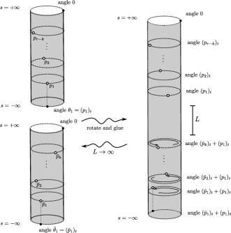
Figure 1. The gluing map for an angle-decorated cylinder rotates all of the angles of the bottom cylinder by the first angle of the top cylinder as in (4.36).

More simply, in the glued surface, the list of incremental angles $(\kappa_{1}^{inc,glued},\ldots,\kappa_{r}^{inc,glued})$ is equal to the concatenation of the lists of incremental angles of the original bottom and top surfaces, $(\bar{\kappa}_{1}^{inc},\bar{\kappa}_{2}^{inc},\ldots,\bar{\kappa}_{k}^{inc},\kappa_{1}^{inc},\kappa_{2}^{inc},\ldots,\kappa_{r-k}^{inc})$.

The compactification $\overline{\mathcal{M}}_{r}$ thus has codimension-1 boundary covered by the images of the natural inclusion maps

(4.37) $$\overline{\mathcal{M}}_{r-k}\times\overline{\mathcal{M}}_{k} \longrightarrow\partial\overline{\mathcal{M}}_{r},\ 0<k<r$$

(4.38) $$\overline{\mathcal{M}}_{r}^{i,i+1} \longrightarrow\partial\overline{\mathcal{M}}_{r},\ 1\leq i<r,$$

where $\overline{\mathcal{M}}_{r}^{i,i+1}$ denotes the compactification of the locus where $i$th and $i+1$st heights are coincident

(4.39) $$\mathcal{M}_{r}^{i,i+1}:=\{C\in\mathcal{M}_{r}\ |\ h_{i}=h_{i+1}\}.$$

With regards to the above stratum, for $r>1$ there is a projection map which will be relevant, a version of the forgetful map which remembers only the first of the angles with coincident heights:

(4.40) $$\begin{split}\pi_{i}:\mathcal{M}_{r}^{i,i+1}&\longrightarrow\mathcal{M}_{r-1}\\ (h_{1},\ldots,h_{i},h_{i+1}=h_{i},h_{i+2},\ldots,h_{r})&\longmapsto(h_{1},\ldots,h_{i},h_{i+2},\ldots,h_{r})\\ (\theta_{1},\ldots,\theta_{i},\theta_{i+1},\ldots,\theta_{r})&\longmapsto(\theta_{1},\ldots,\theta_{i-1},\theta_{i},\widehat{\theta_{i+1}},\theta_{i+2},\ldots,\theta_{r}).\end{split}$$

$\pi_{i}$ is compatible with the choice of positive and negative ends (4.33)-(4.34) and hence $\pi_{i}$ extends to compactifications

(4.41) $$\pi_{i}:\overline{\mathcal{M}}_{r}^{i,i+1}\rightarrow\overline{\mathcal{M}}_{r-1}.$$

We will equip each $r$-point angle-rotated cylinder $\tilde{C}:=(C,p_{1},\ldots,p_{r})$ with perturbation data for Floer’s equation or a Floer datum in the sense of the last section, which consists of

• The positive and negative cylindrical ends on $\epsilon^{\pm}:C^{\pm}\rightarrow C$ chosen in (4.33)-(4.34).

• The one-form on $C$ given by $\alpha=dt$.

• A surface-dependent Hamiltonian $H_{\tilde{C}}:C\rightarrow\mathcal{H}(M)$ compatible with the positive and negative cylindrical ends, meaning that

  (4.42) $$(\epsilon^{\pm})^{*}H_{\tilde{C}}=H_{t},$$

  where $H_{t}$ was the previously chosen Hamiltonian.

• A surface dependent almost complex structure $J_{\tilde{C}}:C\rightarrow\mathcal{J}_{1}(M)$ also compatible with $\epsilon^{\pm}$, meaning that

  (4.43) $$(\epsilon^{\pm})^{*}J_{\tilde{C}}=J_{t}$$

  for our previously fixed choice $J_{t}$.

A choice of Floer data for the $S^{1}$-action is an inductive (smoothly varying) choice of Floer data, for each $r$ and each representative $S=(C,p_{1},\ldots,p_{r})$ of $\overline{\mathcal{M}}_{r}$, satisfying the following consistency conditions at boundary strata:

(4.44) At a boundary stratum (4.37), the datum chosen coincides with the product of

Floer data already chosen on lower-dimensional spaces.

(4.45) At a boundary stratum (4.38), the Floer data coincides with the pull back, via the

forgetful map $$\pi_{i} \overline{\mathcal{M}}_{r-1}$$ defined in (4.41) of the Floer data chosen on .

Inductively, since the space of choices at each level is non-empty and contractible (and since the consistency conditions are compatible along overlapping strata), universal and consistent choices of Floer data exist. From the gluing map, a representative $S$ sufficiently near the boundary strata (4.37) inherits cylindrical regions, also known as thin parts, which are the surviving images of the cylindrical ends of lower-dimensional strata. Together with the cylindrical ends of $S$, this determines a collection of cylindrical regions:

Definition 9.

Given a fixed positive constant $\delta$, the ($\delta$-spaced) rotated cylindrical regions for an $r$-point angle-decorated cylinder $(C,p_{1},\ldots,p_{r})$ consist of the following cylindrical ends and finite cylinders (where $h_{i}=(p_{i})_{s}$ and $\theta_{i}=(p_{i})_{t}$):

• The top cylinder

  (4.46) $$\begin{split}\epsilon^{+}:[0,\max(top(C)-(h_{r}+\delta),0)]\times S^{1}&\rightarrow C\\ (s,t)&\mapsto(\min(s+h_{r}+\delta,top(C)),t)\\ \end{split}$$

• The bottom cylinder

  $$\begin{split}\epsilon^{-}:[\min(bottom(C)-(h_{1}-\delta),0),0]\times S^{1}&\rightarrow C\\ (s,t)&\mapsto(\max(s-(h_{1}-\delta),bottom(C)),t+\theta_{1})\\ &=(\max(s-(h_{1}-\delta),bottom(C)),t+\sum_{j=1}^{r}\kappa_{i})\end{split}$$

• For any $1\leq i\leq r-1$ satisfying $h_{i+1}-h_{i}>2\delta$, the $i$th thin part

  (4.47) $$\begin{split}\epsilon_{i}:[h_{i}+\delta,h_{i+1}-\delta]\times S^{1}&\rightarrow C\\ (s,t)&\mapsto(s,t+\eta_{i})\end{split}$$

Note that a given $r$-point angle-decorated cylinder may not have an the $i$th thin part, for a given $i\in[1,r-1]$, and indeed may not have any thin parts. The consistency conditions at boundary strata can be ensured in particular by requiring that for any ($\delta$-spaced) rotated cylindrical region $\epsilon:C^{\prime}\rightarrow C$ of sufficiently large length (greater than some fixed $L$, say $L=3\delta$) associated to $(C,p_{1},\ldots,p_{r})$ and $\delta$, we have that

(4.48) $$\epsilon^{*}(K_{C},J_{C})=(K_{t},J_{t}).$$

Given the cylindrical regions of Definition 9, this would imply the following condition on $(K_{C},J_{C})$ (assuming $L\gg 3\delta$): for $z=(s,t)\in C$

(4.49) $$\begin{split}(K_{z},J_{z})&=(K_{t},J_{t})\ \textrm{ for }s>h_{r}+\delta;\\ (K_{z},J_{z})&=(\epsilon^{-})^{*}(K_{t},J_{t})=(K_{t+\theta_{1}},J_{t+\theta_{1}})\ \textrm{ for }s<h_{1}-\delta;\\ (K_{z},J_{z})&=\epsilon_{i}^{*}(K_{z},J_{z})=(K_{t+\theta_{i}},J_{t+\theta_{i}})\textrm{ if }h_{i+1}-h_{i}>3\delta\textrm{ and }s\in[h_{i}+\delta,h_{i+1}-\delta].\end{split}$$

Given a choice of Floer data for the $S^{1}$-action and a pair of asymptotics $(x^{+},x^{-})\in\mathcal{O}$ for each $k\geq 1$ there is an associated parametrized moduli space of Floer cylinders with source an arbitrary element of $S\in\mathcal{M}_{r}$ (where the Floer equation is with respect to the Hamiltonian $H_{S}$ and $J_{S}$, with asymptotics $(x^{+},x^{-})$:

(4.50) $$\mathcal{M}_{r}(x^{-};x^{+}):=\{S=(C,p_{1},\ldots,p_{r})\in\mathcal{M}_{r},\ u:C\rightarrow M\ |\ \begin{cases}\lim_{s\rightarrow\pm\infty}(\epsilon^{\pm})^{*}u(s,\cdot)&=x^{\pm}\\ (du-X_{H_{S}}\otimes dt)^{(0,1)_{S}}&=0.\end{cases}\}$$

The consistency condition imposes that the boundary of the Gromov bordification $\overline{\mathcal{M}}_{r}(x^{-};x^{+})$ is covered by the images of the natural inclusions

(4.51) $$\overline{\mathcal{M}}_{r-k}(y;x^{+})\times\overline{\mathcal{M}}_{k}(x^{-};y)\rightarrow\partial\overline{\mathcal{M}}_{r}(x^{-};x^{+})$$

(4.52) $$\overline{\mathcal{M}}_{r}^{i,i+1}(x^{-};x^{+})\rightarrow\partial\overline{\mathcal{M}}_{r}(x^{-};x^{+}),$$

along with the usual semi-stable strip breaking boundaries

(4.53) $$\begin{split}\overline{\mathcal{M}}(y;x^{+})\times\overline{\mathcal{M}}_{r}(x^{-};y)&\rightarrow\partial\overline{\mathcal{M}}_{r}(x^{-};x^{+})\\ \overline{\mathcal{M}}_{r}(y;x^{+})\times\overline{\mathcal{M}}(x^{-};y)&\rightarrow\partial\overline{\mathcal{M}}_{r}(x^{-};x^{+})\end{split}$$

Remark 40 (Floer data in the Liouville case).

Continuing Remark 38, when $M$ is Liouville we impose the following further constraint on Floer data:

(4.54) $$\begin{split}&\textrm{$H_{\tilde{C}}$ is equal to $r^{2}$ or $-\lambda r$ (depending on whether we are in the setting of \S\ref{subsubsec:sh} or \S\ref{subsubsec:relh})}\\ &\textrm{at infinitely many levels of $r$ tending to $\infty$, and $J_{\tilde{C}}$ is (rescaled) contact type near $\infty$.}\end{split}$$

(in fact, in the setting of §4.1.2 we can take $H_{\tilde{C}}$ to be simply equal to $-\lambda r$ for all $r$ outside of a compact set). By e.g., [Abouzaid:2010ly]*Lemma 7.2 or [Abouzaid:2010kx]*§B, this hypothesis implies that sequences of curves with fixed asymptotics cannot escape to $\infty$ in $M$, and that $\mathcal{M}_{r}(x^{-};x^{+})$ given a fixed $x^{+}$ is non-empty for only finitely many $x^{-}$, both necessary inputs to verifying Assumption 1.

In the ${\mathbb{Z}}$-graded case, the virtual dimension of (every component of) $\overline{\mathcal{M}}_{r}(x^{-};x^{+})$ is

(4.55) $$\deg(x^{+})-\deg(x^{-})+(2r-1);$$

in the ${\mathbb{Z}}/2$-graded case every component has virtual dimension of the above parity. By Assumption 1 for a generic fixed choice of Floer data for the $S^{1}$-action (satisfying Remark 40 in the Liouville case), the components of virtual dimension $\leq 1$ of the moduli spaces $\overline{\mathcal{M}}_{r}(x^{-};x^{+})$ are compact manifolds-with-boundary of the correct (expected) dimension. As usual, signed counts of rigid elements of this moduli space for varying $x^{+}$ and $x^{-}$ (using induced maps on orientation lines, twisted as in the differential by $(-1)^{\deg(x_{+})}$—see (4.5)) give the matrix coefficients for the overall map

(4.56) $$\delta_{r}:CF^{*}(M)\rightarrow CF^{*-2r+1}(M).$$

In the degenerate case $r=0$ we define $\delta_{0}$ to be the (already defined) differential:

(4.57) $$\delta_{0}:=d:CF^{*}(M)\to CF^{*+1}(M).$$

Lemma 6.

For each $r$,

(4.58) $$\sum_{i=0}^{r}\delta_{i}\delta_{r-i}=0.$$

Proof.

The counts of rigid elements associated to the boundary of 1-dimensional components of $\partial\overline{\mathcal{M}}_{r}(x^{+};x^{-})$, along with a description of this codimension 1 boundary (4.51)-(4.53) immediately implies that

(4.59) $$(\sum_{i=1}^{r}\delta_{i}\delta_{r-i})+(\sum_{i}\delta_{r}^{i,i+1})+(d\delta_{r}+\delta_{r}d)=0,$$

where $\delta_{r}^{i,i+1}$ for each $i$ is the operation associated to the moduli space of maps (4.52). (Observe that $\delta_{2}^{1,2}$ is precisely the operation $\delta_{2}^{naive}$ from §4.2). Note that the consistency condition (4.45) implies that the Floer datum chosen for any element $S\in\mathcal{M}_{r}^{i,i+1}$ only depends on $\pi_{i}(S)$, where the forgetful map $\pi_{i}:\mathcal{M}_{r}^{i,i+1}\rightarrow\mathcal{M}_{r-1}$ has 1-dimensional fibers. Hence given an element $(S,u)\in\overline{\mathcal{M}}_{r}^{i,i+1}(x^{-};x^{+})$, it follows that $(S^{\prime},u)\in\overline{\mathcal{M}}_{r}^{i,i+1}(x^{-};x^{+})$ for all $S^{\prime}\in\pi_{i}^{-1}\pi_{i}(S)$. In other words, elements of $\overline{\mathcal{M}}_{r}^{i,i+1}(x^{-};x^{+})$ are never rigid, so the associated operation $\delta_{r}^{i,i+1}$ is zero. ∎

By definition we conclude:

Corollary 4.

The pair $(CF^{*}(M;H_{t},J_{t}),\{\delta_{r}\}_{r\geq 0})$ as defined above forms an $S^{1}$-complex, in the sense of Definition 2.∎

By using continuation maps parametrized by various $(S^{1})^{r}\times(0,1]^{r}$ (or equivalently, by spaces of angle-decorated cylinders that are not quotiented by overall ${\mathbb{R}}$-translation), one can prove that

Proposition 5.

Any continuation map $f:CF^{*}(M,H_{1})\to CF^{*}(M,H_{2})$ enhances to a homomorphism $\mathbf{F}$ of $S^{1}$-complexes (which is in particular a quasi-isomorphism if $f$ is). Moreoever, this homomorphism is canonical up to homotopy, in the sense that any two homomorphisms $\mathbf{F}$ and $\mathbf{F}^{\prime}$ enhancing $f$ constructed geometrically from parametrized continuation maps differ by an exact pre-morphism of $S^{1}$-complexes (also constructed geometrically). ∎

We omit the proof, which is standard (see e.g., [Zhao:2019aa] though note some notational differences). In particular, the $S^{1}$-complex defined on the symplectic co-chain complex $SC^{*}(M)$ or the Hamiltonian Floer complex (with small negative slope if $M$ is non-compact) is an invariant of $M$, up to quasi-isomorphism.

Remark 41 (Relation to earlier definitions in the literature).

In [Bourgeois:2012fk] three different definitions of $S^{1}$-equivariant symplectic cohomology are considered and shown to be equivalent; one of the definitions involves taking the $S^{1}$-equivariant homology associated to a certain $S^{1}$-complex defined on $CF^{*}(M)=SC^{*}(M)$ ([Bourgeois:2012fk]*Prop. 2.19). After normalizing for differing conventions (e.g., homological versus cohomological conventions for Floer theory, and the fact that their $u^{-1}$ is our $u$), it is direct to see that the $S^{1}$-complex constructed therein coincides up to equivalence with the one here (and even agrees on the chain level, seeing as the choices of Floer data chosen in that paper constitute a choice of Floer data for the $S^{1}$-action in our sense; compare e.g., [Bourgeois:2012fk]*Fig. 1 with (4.49)).

4.4. The circle action on the interior

From the formal point of view of Floer homology of $M$ as the Morse homology of an action functional on the free loop space $\mathcal{L}M$, one would expect the contributions coming from constant loops to be acted on trivially by the $C_{-*}(S^{1})$ action (which comes from rotation of free loops). This is indeed the case, as we now review.

Suppose that the Hamiltonian $H_{t}$ defining $CF^{*}(M)$ is chosen to be $C^{2}$-small, time-independent, and Morse in the compact region of $\bar{M}$ (which recall equals $M$ if $M$ is compact). Then, Floer proved that all orbits of $H_{t}$ inside $\bar{M}$ are (constant orbits at) Morse critical points of $H$, and all Floer cylinders between such orbits which remain in $\bar{M}$ are in fact Morse trajectories of $H$ [Floer:1989aa].

Let $C_{Morse}(H)$ denote the Morse complex of $H$. In the setting where $H$ is as in §4.1.2 ($M$ can be Liouville or compact), all contributions to $CF^{*}(M)$ (both orbits and cylinders) come from $\bar{M}$, so Floer’s argument gives an isomorphisms

(4.60) $$C_{Morse}(H)\cong CF^{*}(M)$$

In the setting where $H$ is quadratic at infinity (and $M$ is Liouville) as in §4.1.1, one can ensure the collection of orbits coming from $\bar{M}$ is an action-filtered subcomplex (and e.g., the integrated maximum principle will ensure that all cylinders between such orbits lie in $\bar{M}$). Hence, there is an inclusion of subcomplexes

(4.61) $$C_{Morse}(H)\to SC^{*}(M),$$

which, under smallness constraints on the Floer data for the $S^{1}$-action gives an $S^{1}$-subcomplex [Zhao:2019aa]*Lemma 5.4 (meaning the operators $\delta_{k}$ preserve the subcomplex and in fact the action filtration), hence a morphism of $S^{1}$-complexes. We will discuss both of the above cases at once: in either case by considering a Hamiltonian which is $C^{2}$-small on $\bar{M}$ we obtain an inclusion of $S^{1}$-subcomplexes

(4.62) $$C_{Morse}(H)\to CF^{*}(M)$$

with the understanding that in the former case this inclusion is the whole complex.

Lemma 7.

There exists a choice of Floer data for the $S^{1}$-action so that $C_{Morse}(H)$ becomes a trivial $S^{1}$-subcomplex; meaning that the various operators $\delta_{r}$, $r\geq 1$, associated to the $C_{-*}(S^{1})$ action strictly vanish on the subcomplex.

Proof.

By the integrated maximum principle, any Floer trajectory with asymptotics along two generators in $C_{Morse}(H)$ remains in the interior of $\bar{M}$. We can choose the Hamiltonian term of our Floer data on $\mathcal{M}_{r}$ in this region of $M$ to be autonomous (i.e., $t$ and $s$-independent on the cylinder), $C^{2}$-small and Morse — in fact equal to $H$; then Floer’s theorem [Floer:1989aa] again guarantees that any Floer trajectory in $\mathcal{M}_{r}(x^{-};x^{+})$ between Morse critical points $x^{\pm}$ is in fact a Morse trajectory of $H$. It follows that for $x^{+},x^{-}$ critical points of $H$, any element $u=(C,\vec{p})$ in the parametrized moduli space of maps $\overline{\mathcal{M}}_{r}(x^{-};x^{+})$ solves an equation that is independent of the choice of parameter $\vec{p}\in(S^{1})^{r}\times(0,1]^{r-1}$. Namely, $u$ lives in a family of solutions of dimension at least $2r-1$ (given by varying $\vec{p}$), and hence $u$ cannot be rigid. The associated operation $\delta_{r}$, which counts rigid solutions, is therefore zero. ∎

By invariance of the $S^{1}$-complex structure on $CF^{*}(M)$ (up to homotopically canonical quasi-isomorphism as in Proposition 5), we conclude

Corollary 5.

For $M$ compact and admissible, or Liouville with $(H,J)$ as in §4.1.2, $CF^{*}(M)$ is quasi-isomorphic to a trivial $S^{1}$-complex canonically up to homotopy.

Corollary 6.

For $M$ Liouville with $(H,J)$ as in §4.1.1, the inclusion chain map

(4.63) $$C^{*}_{Morse}(M)\rightarrow SC^{*}(M)$$

lifts (cohomologically) canonically to a chain map

(4.64) $$(C_{Morse}(H)[[u]],d_{Morse})=(C_{Morse}(H))^{hS^{1}}\to(SC^{*}(M))^{hS^{1}}=(SC^{*}(M)[[u]],\delta_{eq}).$$

inducing a cohomological map

(4.65) $$H^{*}(M)[[u]]\rightarrow H^{*}(SC^{*}(M)^{hS1}).$$

Remark 42.

Another possibly more direct way of producing the map $H^{*}(M)[[u]]\rightarrow H^{*}(SC^{*}(M)^{hS1})$ is via an $S^{1}$-equivariant enhancement $\widetilde{PSS}$ of the PSS morphism $PSS:C^{*}(M)\to SC^{*}(M)$. We omit a further description here, and simply note that the resulting map can be shown to coincide cohomologically with the map defined above.

Since the $S^{1}$-complex structure on $C^{*}_{Morse}(H)$ is trivial, one can (canonically) split the inclusion of homotopy fixed points map (2.36) $H^{*}(C^{*}_{Morse}(H)^{hS^{1}})\to H^{*}(C^{*}_{Morse}(H))$ by the map

(4.66) $$H^{*}(M)\stackrel{{\scriptstyle[x\mapsto x\cdot 1]}}{{\rightarrow}}H^{*}(M)[[u]];$$

the associated composition

(4.67) $$H^{*}(M)\stackrel{{\scriptstyle[x\mapsto x\cdot 1]}}{{\rightarrow}}H^{*}(M)[[u]]\rightarrow H^{*}(SC^{*}(M)^{hS1})\stackrel{{\scriptstyle[\iota]}}{{\rightarrow}}SH^{*}(M)$$

coincides with the usual map $H^{*}(M)\rightarrow SH^{*}(M)$. In particular, we note that the homotopy fixed point complex of $SC^{*}(X)$ possesses a canonical (geometrically defined) cohomological element,

(4.68) $$\tilde{1}\in H^{*}(SC^{*}(M)^{hS^{1}}),$$

lifting the usual unit $1\in SH^{*}(M)$ (under the map $[\iota]$), defined as the image of $1$ under (4.65).

5. Cyclic open-closed maps

5.1. Open-closed Floer data

Here we review the sort of Floer perturbation data that needs to be specified on the domains appearing in the open-closed map and their cyclic analogues. The main body of our treatment, following §3.3 consists of a (slightly modified) simplification of the setup from [Abouzaid:2010kx] tailored to the case of Fukaya categories of compact admissible $M$; in Remarks 43 and 44 below we will indicate the modifications we need to make (following [Abouzaid:2010kx] and building on Remarks 33, 34, 35, and 36 above) the case of compact Fukaya categories of Liouville manifolds (minor modifications) or wrapped Fukaya categories (slightly more involved modifications). There is one notable deviation from [Abouzaid:2010kx] in that we allow our interior marked point to have a varying asymptotic marker and choose Floer data depending on this choice (as is done in constructions of BV-type operations in Hamiltonian Floer theory involving such asymptotic markers, see e.g., [Seidel:2010uq, Seidel:2014aa]).

Let $S$ be a disc with $d$ boundary punctures $z_{1},\ldots,z_{d}$ (labeled in counterclockwise order) marked as positive and an interior marked point $p$ removed, marked as either positive or negative; for the main body of the construction $p$ is negative. We also equip the interior marked point $p$ with an asymptotic marker, that is a half-line $\tau_{p}\in T_{p}S$ (or equivalently an element of the unit tangent bundle, defined with respect to some metric). Call any such $S=(S,z_{1},\ldots,z_{d},p,\tau_{p})$ an open-closed framed disc.

In addition to the notation for semi-infinite strips (3.38) - (3.39), we use the following notation to refer to the positive and negative semi-infinite cylinder:

(5.1) $$A_{+} :=[0,\infty)\times S^{1}$$

(5.2) $$A_{-} :=(-\infty,0]\times S^{1}$$

A Floer datum on a stable open-closed framed disc $S$ consists of the following choices on each component:

1. A collection of strip-like or cylindrical ends $\mathfrak{S}$ around each boundary or interior marked point respectively of sign matching the sign of the marked point; strip-like ends were defined in §3.3 and a (positive resp. negative) cylindrical end is map

   $$\begin{split}\delta^{\pm}_{j}:A_{\pm}&\rightarrow S\end{split}$$

   (so for the main body of the construction we use a negative cylindrical end around $p$). All of the strip-like ends around each of the $z_{i}$ should be positive, and all (strip-like or cylindrical) ends should have disjoint image in $S$. The cylindrical end around $p$ should further should be compatible with the asymptotic marker, meaning the points with angle zero should asymptotically approach the marker:

   (5.3) $$\lim_{s\rightarrow\pm\infty}\delta^{\pm}(s,0)=\tau_{p}.$$

2. A one-form $\alpha_{S}$ on $S$, an $S$-dependent Hamiltonian function $H_{S}$ on $M$, and an $S$-dependent almost-complex structure $J_{S}$ on $M$, such that on each strip-like end these data pull back to a given fixed $(dt,H_{t},J_{t})$ (which we used to define Lagrangian Floer homology chain-complexes) and on the cylindrical end this data pulls back to a given fixed $(dt,H_{t}^{cyl},J_{t}^{cyl})$ which we used to define our Hamiltonian Floer homology chain complex (note: in many cases we could further simplify and choose $(H_{t}^{cyl},J_{t}^{cyl})=(H_{t},J_{t})$ given a sufficiently generic choice of $(H_{t},J_{t})$)

Given a stable open-closed framed disc $S$ equipped with a Floer datum $F_{S}$, a collection of Lagrangians $\{L_{0},\ldots,L_{d-1}\}$, and asymptotics $\{x_{1},\ldots,x_{d};y\}$ with $x_{i}$ a chord between $L_{i-1}$ and $L_{i\textrm{ mod }d}$, a map $u:S\rightarrow M$ satisfies Floer’s equation for $F_{S}$ with boundary and asymptotics $\{L_{0},\ldots,L_{d-1}\},\{x_{1},\ldots,x_{d};y\}$ if

(5.4) $$(du-X_{S}\otimes\alpha_{S})^{0,1}=0\textrm{ using the Floer data given by $F_{S}$}$$

(meaning $X_{S}$ is the Hamiltonian vector field associated to $H_{S}$, and $0,1$ parts are taken with respect to $J_{S}$), and

(5.5) $$\begin{cases}u(z)\in L_{i}&\textrm{ if $z\in\partial S$ lies counterclockwise from $z_{i}$ and clockwise from $z_{i+1\ \mathrm{mod}\ d}$ }\\ \lim_{s\rightarrow+\infty}u\circ\epsilon^{k}(s,\cdot)=x_{k}&\\ \lim_{s\rightarrow\mp\infty}u\circ\delta(s,\cdot)=y&\end{cases}$$

(here $\epsilon^{k}$ denotes the $k$th strip-like end, $\delta$ denotes the cylindrical end, and the sign $\mp$ in the last line is $-$ if $\delta$ is a negative end — which is the case for the main body of the construction — and $+$ if $\delta$ is a positive end).

Remark 43 (Floer data for compact Lagrangians in Liouville manifolds).

If $M$ is Liouville and we are studying the Fukaya category of compact exact Lagrangians, then we take $H_{t}^{cyl},J_{t}^{cyl}$ (the data required to define Floer cohomology) as in §4.1.2 and we again impose the additional requirements on Floer data described in Remark 34, As before the $H_{t}^{cyl},J_{t}^{cyl}$ and more restrictive types of Floer data chosen for wrapped Fukaya categories in Remark 44 below would also work. The ability to choose $H_{t}^{cyl}$ and $J_{t}^{cyl}$ as in §4.1.2 is indicative of a more general freedom in the Floer data here, which also will allow us later to define operations in which the interior marked point (and all boundary marked points) are positive (see §5.6.2).

Remark 44 (Floer data and Floer’s equation for wrapped Fukaya categories).

Almost exactly as in Remark 35, and following [Abouzaid:2010kx] in order to associate operations between the wrapped Fukaya category and symplectic cohomology, one needs to make the following modifications to the notion of Floer data. First, one takes $H_{t}^{cyl},J_{t}^{cyl}$ to be the data defining the symplectic co-chain complex as in §4.1.1. Then one equips $S$ with strip-like and cylindrical ends as above. Let $\psi^{\rho}$ as before denote the time $\log(\rho)$ Liouville flow on $M$. The modifications to the Floer data are:

• Extra choices of weights and time-shifting maps: Exactly as in Remark 35, one associates a weight $w_{k}\in{\mathbb{R}}_{>0}$ to each boundary or interior marked point and a time-shifting map $\rho_{S}:\partial S\to{\mathbb{R}}_{>0}$ agreeing with $w_{k}$ near the $k$th strip-like end.

• Modified requirements on one-form: The 1-form $\alpha_{S}$ should be subclosed meaning $d\alpha_{S}\leq 0$, restrict to 0 along $\partial S$, and restrict to $w_{k}dt$ on each (strip-like or cylindrical) end (as in item 2 of Remark 35). It follows by Stokes’ theorem that the weight at the (output) cylindrical end should be greater than the sum of weights over all (input) strip-like ends. In particular, it is not possible for $\alpha_{S}$ to be subclosed and restrict to 0 along $\partial S$, conditions necessary to appeal to the integrated maximum principle if the interior marked point were also positive. (This is a reflection of the fact that wrapped Fukaya categories do not admit geometric operations with no outputs.)

• Modified requirements on Hamiltonians, as in item 3 of Remark 35: The Hamiltonian term should pull back to $\frac{H\circ\psi^{w_{k}}}{w_{k}^{2}}$ along any strip-like end and to $\frac{H^{cyl}\circ\psi^{w_{k}}}{w_{k}^{2}}$ along the cylindrical end. The Hamiltonian term should also be quadratic at infinitely many levels of (3.32) tending to infinity (this is a slight weakening of Remark 35 coming from the fact that the Hamiltonian used to define $SC^{*}(X)$ is not quadratic at every level near infinity due to (4.7)).

• Modified requirements on almost complex structures, as in item 4 of Remark 35 The almost-complex structure should be contact-type at infinity and pull back to $(\psi^{w_{k}})^{*}J_{t}$ along each strip-like end and $(\psi^{w_{k}})^{*}J_{t}^{cyl}$ along the cylindrical end.

Exactly as in Remark 35, there is a rescaling action on the space of such Floer data, and we will relax any consistency requirement imposed on Floer data to allow for an arbitrary rescaling when equating different choices of Floer data. Finally, we note the slight modifications to the boundary and asymptotic conditions of Floer’s equation (5.5), following Remark 36: on the boundary component of $\partial S$ lying counterclockwise from $z_{i}$ and clockwise from $z_{i+1\textrm{ mod }d}$ we impose the moving boundary condition $u(z)\in(\psi^{\rho_{S}(z)})^{*}L_{i}$, on the $k$th strip-like end we impose $\lim_{s\rightarrow+\infty}u\circ\epsilon^{k}(s,\cdot)=(\psi^{w_{k}})^{*}x_{k}$, and on the cylindrical end, we impose $\lim_{s\rightarrow-\infty}u\circ\delta(s,\cdot)=(\psi^{w})^{*}y$ where $w$ is the weight associated to the interior puncture $p$.

Exactly as in the proof of Lemma 4, the constraints to Floer data in the Liouville case made in the above two remarks help ensure Assumption 1 holds for associated moduli spaces.

5.2. Non-unital open-closed maps

We begin by constructing a variant of the open-closed map of [Abouzaid:2010kx] with source the non-unital Hochschild complex of (3.11), which we call the non-unital open-closed map (and indicate by $\mathcal{OC}$ or $\mathcal{OC}^{nu}$)

(5.6) $$\mathcal{OC}:=\mathcal{OC}^{nu}:\mathrm{CH}^{nu}_{*-n}(\mathcal{F})\longrightarrow CF^{*}(M).$$

This map actually has a straightforward explanation from the perspective of Remark 26: we define the map $\mathcal{OC}$ from $\widetilde{\mathrm{CH}}_{*}(\mathcal{F})$ by counting discs with an arbitrary number of boundary punctured and one interior puncture asymptotic to an orbit (as in [Abouzaid:2010kx] with the proviso that we treat the formal elements $e_{L}^{+}$ as “fundamental class $[L]$ point constraints (i.e., empty constraints)”: we fill back in the relevant boundary puncture and impose no constraints on that marked point. With respect to the decomposition (3.11), we define a pair of maps

(5.7) $$\check{\mathcal{OC}}\oplus\hat{\mathcal{OC}}:\mathrm{CH}_{*}(\mathcal{F})\oplus\mathrm{CH}_{*}(\mathcal{F})[1]\rightarrow CF^{*}(M)$$

giving the left and right component of the non-unital open-closed map

(5.8) $$\begin{split}\mathcal{OC}:\mathrm{CH}^{nu}_{*-n}(\mathcal{F})&\longrightarrow SC(M),\\ (x,y)&\longmapsto\check{\mathcal{OC}}(x)+\hat{\mathcal{OC}}(y).\end{split}$$

Since the left (check) factor is equal to the usual cyclic bar complex for Hochschild homology, $\check{\mathcal{OC}}$ will be defined exactly as the open-closed map is defined in [Abouzaid:2010kx] (briefly recalled below), and the new content is the map $\hat{\mathcal{OC}}$. We will define $\hat{\mathcal{OC}}$ below (and recall the definition of $\check{\mathcal{OC}}$) and prove, extending [Abouzaid:2010kx] that

Lemma 8.

$\mathcal{OC}$ is a chain map of degree $n$.

We note a notational difference from [Abouzaid:2010kx], which uses $\mathcal{OC}$ to refer to what we call here $\check{\mathcal{OC}}$; in contrast in this paper we use $\mathcal{OC}$ exclusively to refer to the (non-unital) open-closed map $\mathcal{OC}=\mathcal{OC}^{nu}:=\check{\mathcal{OC}}\oplus\hat{\mathcal{OC}}$ with domain the non-unital Hochschild complex. Of course, the two maps $\mathcal{OC}$ and $\check{\mathcal{OC}}$ are homologically the same. That is, assuming Lemma 8,

Corollary 7.

As homology level maps, $[\mathcal{OC}]=[\check{\mathcal{OC}}]$.

Proof.

By construction, the chain level map $\check{\mathcal{OC}}$ constructed in [Abouzaid:2010kx] factors as

(5.9) $$\mathrm{CH}_{*-n}(\mathcal{F})\subset\mathrm{CH}_{*-n}^{nu}(\mathcal{F})\stackrel{{\scriptstyle\mathcal{OC}}}{{\longrightarrow}}CF^{*}(M).$$

The first inclusion is a quasi-isomorphism by Lemma 2, since $\mathcal{F}$ is known to be cohomologically unital. ∎

The moduli space controlling the operation $\check{\mathcal{OC}}$, denoted

(5.10) $$\overline{\check{\mathcal{R}}}_{d}^{1}$$

is the (Deligne-Mumford compactification of the) abstract moduli space of discs with $d$ boundary positive punctures $z_{1},\ldots,z_{d}$ labeled in counterclockwise order and 1 interior negative puncture $z_{out}$, with an asymptotic marker $\tau_{out}$ at $z_{out}$ pointing towards $z_{d}$. The space (5.10) has a manifold with corners structure, with boundary strata described in [Abouzaid:2010kx]*§C.3 (there, the space is called $\overline{\mathcal{R}}_{d}^{1}$)–in short, codimension one strata consist of disc bubbles containing any cyclic subsequence of $k$ inputs attached to an element of $\check{\mathcal{R}}_{d-k+1}^{1}$ at the relative position of this cyclic subsequence. Orient the top stratum $\check{\mathcal{R}}_{d}^{1}$ by trivializing it, sending $[S]$ to the unit disc representative $S$ with $z_{d}$ and $z_{out}$ fixed at 1 and 0, and taking the orientation induced by the (angular) positions of the remaining marked points:

(5.11) $$-dz_{1}\wedge\cdots\wedge dz_{d-1}.$$

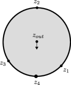
Figure 2. A representative of an element of the moduli space $\check{\mathcal{R}}^{1}_{4}$ with special points at 0 (output), $-i$.

The moduli space controlling the new map $\hat{\mathcal{OC}}$ is nearly identical to $\check{\mathcal{R}}_{d}^{1}$, but there is additional freedom in the direction of the asymptotic marker at the interior puncture $z_{out}$. The top (open) stratum is easiest to define: let

(5.12) $$\mathcal{R}_{d}^{1,free}$$

be the moduli space of discs with $d$ positive boundary punctures and one interior negative puncture as in $\check{\mathcal{R}}_{d}^{1}$, but with the asymptotic marker $\tau_{out}$ pointing anywhere between $z_{1}$ and $z_{d}$.

Remark 45.

There is a delicate point in naively compactifying $\mathcal{R}_{d}^{1,free}$: on any formerly codimension 1 stratum in which $z_{1}$ and $z_{d}$ bubble off, the position of $\tau_{out}$ becomes fixed too, and so the relevant stratum actually should have codimension 2 (and hence does not contribute to the codimension-1 boundary equation for $\hat{\mathcal{OC}}$. Moreoever, there is no nice corner chart near this stratum). For technical convenience, we pass to an alternate, larger (blown-up) model for the compactification in which these strata have codimension 1 but consist of degenerate contributions.

In light of Remark 45, we use (5.12) as motivation and instead define

(5.13) $$\hat{\mathcal{R}}_{d}^{1}$$

to be the abstract moduli space of discs with $d+1$ boundary punctures $z_{f}$, $z_{1}$, …, $z_{d}$ and an interior puncture $z_{out}$ with asymptotic marker $\tau_{out}$ pointing towards the boundary point $z_{f}$, modulo automorphism. We mark $z_{f}$ as “auxiliary,” but otherwise the space is abstractly isomorphic to $\check{\mathcal{R}}^{1}_{d+1}$. Identifying $\hat{\mathcal{R}}_{d}^{1}$ with the space of unit discs with $z_{out}$ and $z_{f}$ fixed at 1 and 0, the remaining (angular) positions of $z_{1},\ldots,z_{d}$ determine an orientation

(5.14) $$-dz_{1}\wedge\cdots\wedge dz_{d}.$$

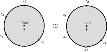
Figure 3. A representative of an element of the moduli space $\mathcal{R}^{1}_{4,free}$ and the corresponding element of $\hat{\mathcal{R}}_{4}^{1}$.

The forgetful map

(5.15) $$\pi_{f}:\hat{\mathcal{R}}_{d}^{1}\rightarrow\mathcal{R}_{d}^{1,free}$$

puts back in the point $z_{f}$ and forgets it. Since the point $z_{f}$ is recoverable from the direction of the asymptotic marker at $z_{out}$,

Lemma 9.

$\pi_{f}$ is a diffeomorphism.∎

The perspective of the former space (5.13) gives us a model for the compactification

(5.16) $$\overline{\mathcal{R}}_{d}^{1,free}$$

as the ordinary Deligne-Mumford compactification

(5.17) $$\overline{\hat{\mathcal{R}}}_{d}^{1}.$$

We call a component $T$ of a representative $S$ of (5.17) the main component if it contains the interior marked point, and a secondary component if its output is attached to the main component. As a manifold with corners, (5.17) is equal to the compactification $\overline{\check{\mathcal{R}}}_{d+1}^{1}$ except from the point of view of assigning Floer datum, as we will be forgetting the point $z_{f}$ instead of fixing asymptotics for it. It is convenient therefore (for the purpose of indicating choices of Floer data made) to name components of strata containing $z_{f}$ differently. At any stratum:

• we treat the main component (containing $z_{out}$ and $k$ boundary marked points) as belonging to $\overline{\hat{\mathcal{R}}}_{k-1}^{1}$ if it contains $z_{f}$ and $\overline{\check{\mathcal{R}}}_{k}^{1}$ otherwise; and

• If the $i$th boundary marked point of any non-main component was $z_{f}$, we view it as an element of $\mathcal{R}^{k,f_{i}}$, the space of discs with 1 output and $k$ input marked points removed from the boundary, with the $i$th point marked as “forgotten,” constructed in Appendix A.2.

• We treat any other non-main component as belonging to $\mathcal{R}^{k}$ as usual.

Thus, the codimension-1 boundary of the Deligne-Mumford compactification is covered by the natural inclusions of the following strata

(5.18) $$\overline{\mathcal{R}}^{m} \times_{i}\overline{\hat{\mathcal{R}}}_{d-m+1}^{1}\ \ \ 1\leq i<d-m+1$$

(5.19) $$\overline{\mathcal{R}}^{m,f_{k}} \times_{d-m+1}\overline{\check{\mathcal{R}}}^{1}_{d-m+1}\ \ \ 1\leq j\leq m,\ 1\leq k\leq m$$

where the notation $\times_{j}$ means that the output of the first component is identified with the $j$th boundary input of the second. See Figure 4.

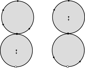
Figure 4. A schematic of the two distinct types of codimension-1 boundary strata of (5.17) in codimension 1. On the left side, corresponding to (5.18), a disc bubble forms involving any collection of boundary marked points not including $z_{f}$. On the right side, corresponding to (5.19), a disc bubble forms involving the point $z_{f}$.

The forgetful map $\pi_{f}$ extends to a map $\overline{\pi}_{f}$ from the compactification $\overline{\hat{\mathcal{R}}}_{d}^{1}$ (to the space of stable framed open-closed discs with $d$ marked points) as follows: $\overline{\pi}_{f}$ puts the auxiliary point $z_{f}$ back in, eliminates any component which is not main or secondary which has only one non-auxiliary marked point $p$, and labels the positive marked point below this component by $p$. Given a representative $S$ of $\overline{\hat{\mathcal{R}}}_{d}^{1}$, we call $\overline{\pi}_{f}(S)$ the associated reduced surface. We will study maps from the associated reduced surfaces $\overline{\pi}_{f}(S)$, parametrized by $S$. To this end, we define a Floer datum on a stable disc $S$ in $\overline{\hat{\mathcal{R}}}_{d}^{1}$ to consist of a Floer datum for the underlying reduced surface $\overline{\pi}_{f}(S)$ in the sense of §5.1.

First, in Appendix A.2 we describe an inductive construction of Floer data for (the underlying reduced surfaces of) the compactified moduli space of discs with a forgotten point $\overline{\mathcal{R}}^{d,f_{i}}$, for every $d$ and $i$ satisfying:

(5.20) $$\begin{split}&\textrm{For $d>2$, the choice of Floer datum on $\mathcal{R}^{d,f_{i}}$ should be pulled back from the forgetful map $\mathcal{R}^{d,f_{i}}\rightarrow\mathcal{R}^{d-1}$. }\\ &\textrm{For $d=2$, the Floer datum on the surface $S$ (with $z_{i}$ forgotten) should be translation invariant.}\end{split}$$

Next, we choose a Floer datum for the non-unital open-closed map which is an inductive set of choices $(\mathbf{D}_{\check{\mathcal{OC}}},\mathbf{D}_{\hat{\mathcal{OC}}})$, for each $d\geq 1$ and every representative $S\in\overline{\check{\mathcal{R}}}_{d}^{1}$, $T\in\overline{\hat{\mathcal{R}}}_{d}^{1}$, of a Floer datum for $S$ and (the associated reduced surface of) $T$ respectively. As usual, these choices should be smoothly varying, and restrict smoothly to previously chosen Floer data on boundary strata. Note that for a given $d$ the boundary strata have components that are either $\overline{\check{\mathcal{R}}}_{d^{\prime}}^{1}$ or $\overline{\hat{\mathcal{R}}}_{d^{\prime}}^{1}$ for $d^{\prime}<d$, a stratum $\mathcal{R}^{d^{\prime}}$ (over which we have chosen a Floer datum for the $A_{\infty}$ structure), or a stratum $\mathcal{R}^{d,f_{i}}$ where we have chosen a Floer datum in Appendix A.2 as described above. (As usual for Liouville manifolds we use the notion of Floer data and consistency described in Remarks 43 or 44 in the wrapped case.) Contractibility of the space of choices at every stage (and consistency of the compatibility conditions imposed at corners) ensures as usual that a Floer datum for the non-unital open-closed map exists.

Fixing such a choice, we obtain, for any $d$-tuple of Lagrangians $L_{0},\ldots,L_{d-1}$, and asympotic conditions $\vec{x}=(x_{d},\ldots,x_{1}),\ x_{i}\in\chi(L_{i-1},L_{i\textrm{ mod }d})$, $y_{out}\in\mathcal{O}$ a pair of moduli spaces

(5.21) $$\check{\mathcal{R}}_{d}^{1}(y_{out};\vec{x})$$

(5.22) $$\hat{\mathcal{R}}_{d}^{1}(y_{out};\vec{x}),$$

of parametrized families of solutions to Floer’s equation

(5.23) $$\{(S,u)|S\in\check{\mathcal{R}}_{d}^{1}:u:S\rightarrow M,(du-X\otimes\alpha)^{0,1}=0\textrm{ using the Floer datum given by $\mathbf{D}_{\check{\mathcal{OC}}}(S)$}\}$$

(5.24) $$\{(S,u)|S\in\hat{\mathcal{R}}_{d}^{1},u:\pi_{f}(S)\rightarrow M|(du-X\otimes\alpha)^{0,1}=0\textrm{ using the Floer datum given by $\mathbf{D}_{\hat{\mathcal{OC}}}(S)$}\}$$

satisfying asymptotic and boundary conditions (in either case) as in (5.5) (with the modification for wrapped Fukaya categories involving Liouville rescalings described in Remark 44). The expected dimension of every component of (5.21) and (5.22) respectively, is (in the ${\mathbb{Z}}$-graded case), or agrees mod 2 with (in the ${\mathbb{Z}}/2$-graded case):

(5.25) $$\deg(y_{out})-n+d-1-\sum_{k=1}^{d}\deg(x_{k});$$

(5.26) $$\deg(y_{out})-n+d-\sum_{k=1}^{d}\deg(x_{k}).$$

As usual there are Gromov-type bordifications

(5.27) $$\overline{\check{\mathcal{R}}}_{d}^{1}(y_{out};\vec{x});$$

(5.28) $$\overline{\hat{\mathcal{R}}}_{d}^{1}(y_{out};\vec{x}),$$

which allow semi-stable breakings, as well as maps from strata corresponding to the boundary strata of $\overline{\check{\mathcal{R}}}_{d}^{1}$ and $\overline{\hat{\mathcal{R}}}_{d}^{1}$.

By Assumption 1, for generic choices of Floer datum for the non-unital open-closed map, the components of (5.27) and (5.28) of virtual dimension $\leq 1$ are compact manifolds-with-boundary of dimension agreeing with virtual dimension. Fix such a Floer datum. At a rigid element $u$ of each of the above moduli spaces, we obtain, using the fixed orientations of moduli spaces of domains (5.11)-(5.14) and [Abouzaid:2010kx]*Lemma C.4, isomorphisms of orientation lines

(5.29) $$(\check{\mathcal{R}}_{d}^{1})_{u}:o_{x_{d}}\otimes\cdots\otimes o_{x_{1}}\rightarrow o_{y_{out}}$$

(5.30) $$(\hat{\mathcal{R}}_{d}^{1})_{u}:o_{x_{d}}\otimes\cdots\otimes o_{x_{1}}\rightarrow o_{y_{out}}.$$

These isomorphisms in turn define the $|o_{y_{out}}|_{\mathbf{k}}$ component of the check and hat components of the non-unital open-closed map with $d$ inputs in the lines $|o_{x_{d}}|_{\mathbf{k}},\ldots,|o_{x_{1}}|_{\mathbf{k}}$, up to a sign twist:

(5.31) $$\begin{split}\check{\mathcal{OC}}_{d}&([x_{d}],\ldots,[x_{1}]):=\\ &\sum_{u\in\overline{\check{\mathcal{R}}}^{d}_{1}(y;x_{d},\ldots,x_{1})\textrm{ rigid}}(-1)^{\check{\star}_{d}}(\check{\mathcal{R}}_{d}^{1})_{u}([x_{d}],\ldots,[x_{1}]),\\ \check{\star}_{d}&:=\deg(x_{d})+\sum_{k=1}^{d}k\deg(x_{k})\end{split}$$

(5.32) $$\begin{split}\hat{\mathcal{OC}}_{d}([x_{d}],\ldots,[x_{1}])&:=\sum_{u\in\overline{\hat{\mathcal{R}}}_{d}^{1}(y_{out};\vec{x})\textrm{ rigid}}(-1)^{\hat{\star}_{d}}(\hat{\mathcal{R}}_{d}^{1})_{u}([x_{d}],\ldots,[x_{1}]),\\ \hat{\star}_{d}&:=\sum_{i=1}^{d}i\cdot\deg(x_{i}).\end{split}$$

By analyzing the boundary of one-dimensional components of the moduli spaces $\overline{\check{\mathcal{R}}}_{d}^{1}(y_{out};\vec{x})$, the consistency condition imposed on Floer data, and a sign analysis, it was proven in [Abouzaid:2010kx] that

Lemma 10 ([Abouzaid:2010kx], Lemma 5.4).

$\mathcal{OC}:=\check{\mathcal{OC}}$ is a chain map of degree $n$; that is $(-1)^{n}d_{CF}\circ\check{\mathcal{OC}}=\check{\mathcal{OC}}\circ b$.∎

Similarly, we prove the following, completing the proof of Lemma 8:

Lemma 11.

The following equation holds:

(5.33) $$(-1)^{n}d_{CF}\circ\hat{\mathcal{OC}}=\check{\mathcal{OC}}\circ d_{\wedge\vee}+\hat{\mathcal{OC}}\circ b^{\prime}$$

Proof.

The consistency condition imposed on Floer data implies that the boundary of the 1-dimensional components of $\overline{\check{\mathcal{R}}}_{d}^{1}(y;\vec{x})$ are covered by the images of the natural inclusions of the rigid (zero-dimensional) components of the moduli spaces of maps coming from the boundary strata (5.18), (5.19) along with (the rigid components of) semi-stable breakings:

(5.34) $$\overline{\hat{\mathcal{R}}}_{d}^{1}(y_{1};\vec{x})\times\overline{\mathcal{M}}(y_{out};y_{1}) \rightarrow\partial\overline{\check{\mathcal{R}}}_{d}^{1}(y_{out};\vec{x})$$

(5.35) $$\overline{\mathcal{R}}^{1}(x;x_{i})\times\overline{\hat{\mathcal{R}}}_{d}^{1}(y_{out};\tilde{\vec{x}}) \rightarrow\partial\overline{\check{\mathcal{R}}}_{d}^{1}(y_{out};\vec{x}),$$

where $\tilde{\vec{x}}$ denotes the collection of inputs $\vec{x}$ with $x_{i}$ replaced with $x$. Let $\mu^{d,i}$ be the operation associated to the space of discs with $i$th point marked as forgotten $\mathcal{R}^{d,f_{i}}$, which is described in detail in Appendix A.2. $\mu^{d,i}$ takes a composable sequence of $d-1$ inputs, separated into an $i-1$ tuple and a $d-i$ tuple; in line with Remark 26 we will use the suggestive notation

(5.36) $$\mu^{d}(x_{d},\ldots,x_{i+1},e^{+},x_{i-1},\ldots,x_{1}):=\mu^{d,i}(x_{d},\ldots,x_{i+1};x_{i-1},\ldots,x_{1})\text{}$$

(recall the abuse of notation $x_{i}:=[x_{i}]$). Then, up to sign, by the standard codimension-1 boundary principle for Floer-theoretic operations, we have shown that

(5.37) $$\begin{split}0=&d_{CF}\hat{\mathcal{OC}}(x_{d},\ldots,x_{1})-\sum_{i,j}(-1)^{\maltese_{1}^{i}}\hat{\mathcal{OC}}(x_{d},\ldots,x_{i+j+1},\mu^{j}(x_{i+j},\ldots,x_{i+1}),x_{i},\cdots,x_{1})\\ &-\sum_{i,j,k}(-1)^{\sharp_{j}^{k}}\check{\mathcal{OC}}(\mu^{j+k+1}(x_{j},\ldots,x_{1},e^{+},x_{d},\ldots,x_{d-k+1}),x_{d-k},\ldots,x_{j+1})\end{split}$$

with desired signs

(5.38) $$\maltese_{m}^{n} =\sum_{j=m}^{n}||x_{i}||$$

(5.39) $$\sharp_{j}^{k} =\maltese_{1}^{j}\maltese_{j+1}^{d}+\maltese_{j+1}^{d}+1.$$

However, as shown in Appendix A.2,

(5.40) $$\mu^{j+k+1}(x_{j},\ldots,x_{1},e^{+},x_{d},\ldots,x_{d-k+1})=\begin{cases}x_{1}&j=1,\ k=0\\ (-1)^{|x_{d}|}x_{d}&j=0,k=1\\ 0&\textrm{otherwise}\end{cases}$$

(in this manner, $e^{+}$, though a formal element, behaves as a strict unit). So if (5.37) held, it would follow that

(5.41) $$\begin{split}d_{CF}\circ\hat{\mathcal{OC}}(x_{d}\otimes\cdots\otimes x_{1})&=(-1)^{||x_{1}||\maltese_{2}^{d}+\maltese_{2}^{d}+1}\check{\mathcal{OC}}(x_{1}\otimes x_{d}\otimes\cdots\otimes x_{2})\\ &+(-1)^{|x_{d}|+\maltese_{1}^{d}+1}\check{\mathcal{OC}}(x_{d}\otimes\cdots\otimes x_{1})+\hat{\mathcal{OC}}\circ b^{\prime}(x_{d}\otimes\cdots\otimes x_{1})\\ &=\check{\mathcal{OC}}((-1)^{\maltese_{1}^{d}+||x_{d}||}(1-t)(x_{d}\otimes\cdots\otimes x_{1}))+\hat{\mathcal{OC}}\circ b^{\prime}(x_{d}\otimes\cdots\otimes x_{1}).\\ &=\left(\check{\mathcal{OC}}\circ d_{\wedge\vee}+\hat{\mathcal{OC}}\circ b^{\prime}\right)(x_{d}\otimes\cdots\otimes x_{1}).\end{split}$$

So we are done if we establish the signs are exactly (5.38)-(5.39).

Using the notation

(5.42) $$\mathcal{OC}(e^{+}\otimes x_{d}\otimes\cdots\otimes x_{1}):=\hat{\mathcal{OC}}(x_{d}\otimes\cdots\otimes x_{1}),$$

where again $e^{+}$ is simply a formal symbol referring to the position of the auxiliary (forgotten) input point, we observe that the equation (5.37) is exactly the equation for $\mathcal{OC}$ being a chain map on inputs of the form $(e^{+}\otimes x_{d}\otimes\cdots\otimes x_{1})$ (where we treat an “$e^{+}$” input as an auxiliary unconstrained point on our domain). The sign verification therefore follows from that of $\check{\mathcal{OC}}$ being a chain map (in [Abouzaid:2010kx]*Lemma 5.4), for we have used identical orientations on the abstract moduli space $\hat{\mathcal{R}}_{d}^{1}$ as on $\check{\mathcal{R}}_{d+1}^{1}$ (identifying $z_{f}$ with $z_{d+1}$), and on $\mathcal{R}^{d,f_{i}}$ as on $\mathcal{R}^{d}$, and we can even insert a formal degree zero orientation line $o_{e^{+}}$ into the procedure for orienting moduli spaces of open-closed maps (see [Abouzaid:2010kx]*§C.6), corresponding to the marked point (obtained by filling in) $z_{f}$. Note that $o_{e^{+}}$, being of degree zero, commutes with everything, and is just used as a placeholder as if we had an asymptotic condition at $z_{f}$. ∎

Proof of Lemma 8.

Given that $\check{\mathcal{OC}}$ is already known to be a chain map by [Abouzaid:2010kx]*Lemma 5.4, repeated as Lemma 10 above, the new part to check is that the $(-1)^{n}d_{CF}\circ\hat{\mathcal{OC}}=\check{\mathcal{OC}}d_{\wedge\vee}+\hat{\mathcal{OC}}\circ b^{\prime}$. This is the content of Lemma 11 above. ∎

5.3. An auxiliary operation

It will be technically convenient to define an auxiliary operation

(5.43) $$\mathcal{OC}^{S^{1}}:\mathrm{CH}_{*-n}(\mathcal{F})\rightarrow CH^{*+1}(M)$$

from the left factor of the non-unital Hochschild complex to Floer co-chains, in which the asymptotic marker $\tau_{out}$ varies freely around the circle. This operation is more easily comparable to the BV operator on Floer cohomology, and moreover, we will show that $\mathcal{OC}^{S^{1}}$ (and $\hat{\mathcal{OC}}$) can be chosen to satisfy the following crucial identity:

Proposition 6.

There is an equality of chain level operations:

(5.44) $$\mathcal{OC}^{S^{1}}=\hat{\mathcal{OC}}\circ B^{nu}.$$

To define (5.43), let

(5.45) $$\mathcal{R}^{S^{1}}_{d}$$

be the abstract moduli space of discs with $d$ boundary positive punctures $z_{1},\ldots,z_{d}$ labeled in counterclockwise order and 1 interior negative puncture $z_{out}$, with an asymptotic marker $\tau_{out}$ at $z_{out}$ (or choice of real half line in $T_{z_{out}}D$) which is free to vary. Equivalently,

(5.46) $$\begin{split}&\textrm{\eqref{S1modulispace} is the space of discs with $z_{1},\ldots,z_{d}$ and $z_{out}$ as before, and an extra auxiliary }\\ &\textrm{interior marked point $p_{1}$ such that, for a representative with $(z_{out},z_{1})$ fixed at $(0,-i)$, }\\ &\textrm{$|p_{1}|=\frac{1}{2}$, and the asymptotic marker $\tau_{out}$ points towards $p_{1}$.}\end{split}$$

By using a representative with fixed $(z_{out},z_{1})$ as above, the argument of $p_{1}$ produces an abstract identification

(5.47) $$\mathcal{R}^{S^{1}}_{d}=\check{\mathcal{R}}^{1}_{d}\times S^{1};$$

using this identification, fix an orientation of (5.47) given by negative the product orientation of (5.11) with the standard counterclockwise orientation on $S^{1}$. The Deligne-Mumford type compactification can thus be thought of as

(5.48) $$\overline{\mathcal{R}_{d}^{S^{1}}}=\overline{\check{\mathcal{R}}}^{1}_{d}\times S^{1}$$

Given an element $S$ of $\mathcal{R}_{d}^{S^{1}}$ and a choice of marked point $z_{i}$ on the boundary of $S$, we say say that $\tau_{out}$ points at $z_{i}$, if, when $S$ is reparametrized so that $z_{1}$ fixed at $-i$ and $z_{out}$ fixed at 0, the vector $\tau_{out}$ is tangent to the straight line from $z_{out}$ to $z_{i}$. Equivalently, for this representative, $z_{out}$, $p_{1}$, and $z_{i}$ are collinear. For each $i$, the locus where $\tau_{out}$ points at $z_{i}$ forms a codimension 1 submanifold, denoted

(5.49) $$\mathcal{R}_{d}^{S^{1}_{i}}.$$

The notion compactifies well; if $z_{i}$ is not on the main component of (5.48) we say $\tau_{out}$ points at $z_{i}$ if it points at the root of the bubble tree $z_{i}$ is on. This compactified locus $\overline{\mathcal{R}_{d}^{S^{1}_{i}}}$ can be identified with $\overline{\mathcal{R}}^{1}_{d}$ via the map

(5.50) $$\tau_{i}:\overline{\mathcal{R}_{d}^{S^{1}_{i}}}\rightarrow\overline{\mathcal{R}}^{1}_{d}$$

which cyclically permutes the labels of the boundary marked points so that $z_{i}$ is now labeled $z_{d}$.

In a similar fashion, we have an invariant notion of what it means for $\tau_{out}$ to point between $z_{i}$ and $z_{i+1}$; this is a codimension 0 submanifold with corners of (5.47), denoted

(5.51) $$\mathcal{R}_{d}^{S^{1}_{i,i+1}}.$$

The compactification has some components that are codimension 1 submanifolds with corners of (5.48), when $z_{i}$ and $z_{i+1}$ both lie on a bubble tree.

Finally, there is a free ${\mathbb{Z}}_{d}$ action generated by the map

(5.52) $$\kappa:\overline{\mathcal{R}_{d}^{S^{1}}}\rightarrow\overline{\mathcal{R}_{d}^{S^{1}}}$$

which cyclically permutes the labels of the boundary marked points; for concreteness, $\kappa$ changes the label $z_{i}$ to $z_{i+1}$ for $i<d$, and $z_{d}$ to $z_{1}$. Note that if, on a given $S$, $\tau_{out}$ points between $z_{i}$ and $z_{i+1}$, then on $\kappa(S)$, $\tau_{out}$ points between $z_{i+1\rm{\ mod\ }d}$ and $z_{i+2\rm{\ mod\ }d}$.

Lemma 12.

The action generated by (5.52) is free and properly discontinuous.

Sketch.

The basic observation arises on the level of uncompactified moduli spaces: since any element of $\mathcal{R}_{d}^{S^{1}}$ has a unit disk representative with $(z_{out},p_{1})$ fixed at $(0,\frac{1}{2})$, the positions of the remaining points identify $\mathcal{R}_{d}^{S^{1}}$ with the space of tuples $(z_{1},\ldots,z_{d})$ of disjoint (cylically ordered) points on $S^{1}$ (without any further quotienting by automorphism). The action of $\kappa$, which cyclically permutes the labels $z_{1},\ldots,z_{d}$ in this identification, evidently acts freely and properly discontinuously on this locus. Similarly, an element of a boundary stratum consists of an element of $\mathcal{R}_{k}^{S^{1}}$ for some $k\leq d$ with some collection of stable disc bubble trees attached to some or all of the marked points of $\mathcal{R}_{k}^{S^{1}}$, so that there are $d$ leaf (non-nodal) boundary marked points, along with a counterclockwise-ordered labeling of these marked points by $z_{1},\ldots,z_{d}$ (note that there is a well-defined cyclic counterclockwise ordering of boundary marked points on any such stable configuration). By using a representative of the main component $\mathcal{R}_{k}^{S^{1}}$ with $(z_{out},p_{1})$ fixed at $(0,\frac{1}{2})$, an explicit analysis shows that the action of (5.52) remains free and properly discontinuous (e.g., to see free, note there is a well-defined “first boundary non-nodal marked point at or counterclockwise from the argument of $p_{1}$”; the action of (5.52) freely permutes the label of this first boundary marked point hence cannot have a fixed point). ∎

The quotient of the action of $\kappa$ consists of the space of discs with $z_{out}$ and $p_{1}$ as before (meaning $z_{out}$ is a negative interior puncture, and $p_{1}$ is an auxiliary interior marked point such that for any representative with $z_{out}$ fixed at 0, $|p_{1}|=\frac{1}{2}$), equipped with $d$ cyclically unordered or unlabeled boundary marked points. Note that on the open-locus $\mathring{\mathcal{R}}_{d}^{S^{1}}$ where $\tau_{out}$ does not point at a boundary marked point, one can choose a labeling by setting the boundary point immediately clockwise of where $\tau_{out}$ points to be $z_{d}$. This induces a diffeomorphism

(5.53) $$\mathring{\mathcal{R}}_{d}^{S^{1}}/\kappa\cong\mathcal{R}_{d}^{1,free}$$

Similarly, on the complementary locus where $\tau_{out}$ points at a boundary marked point, we can similarly choose a labeling by declaring this boundary marked point to be $z_{d}$, giving a diffeomorphism (of this locus) with $\check{\mathcal{R}}_{d}^{1}$.

We now choose Floer perturbation data for the family of moduli spaces $\mathcal{R}_{d}^{S^{1}}$; in fact, it will be helpful to re-choose Floer data for the moduli spaces appearing in the non-unital open-closed map to have extra compatibility. To that end, a BV compatible Floer datum for the non-unital open-closed map is an inductive choice $(\mathbf{D}_{\check{\mathcal{OC}}},\mathbf{D}_{\hat{\mathcal{OC}}},\mathbf{D}_{S^{1}})$ of Floer data where $\mathbf{D}_{\check{\mathcal{OC}}}$ and $\mathbf{D}_{\hat{\mathcal{OC}}}$ is a universal and consistent choice of Floer data for the non-unital open-closed map as before, and $\mathbf{D}_{S^{1}}$ consists of, for each $d\geq 1$ and every representative $S\in\overline{\mathcal{R}_{d}^{S^{1}}}$, a Floer datum for $S$ varying smoothly over the moduli space. Again, these satisfy the usual consistency condition with respect to previously made choices along lower-dimensional strata. Moreover, there are two additional inductive constraints on the Floer data chosen:

(5.54) On the codimension-1 loci $$\overline{\mathcal{R}_{d}^{S^{1}_{i}}} \tau_{out} z_{i}$$ where points at , the Floer datum

should agree with the pullback by $$\tau_{i}$$ of the existing Floer datum

for the (check) open-closed map.

(5.55) The Floer datum should be $$\kappa \kappa$$-equivariant, where is the map (5.52).

Also, there is a final a posteriori constraint on the Floer data for the non-unital open-closed map $\mathbf{D}_{\hat{\mathcal{OC}}}$; for $S\in\overline{\hat{\mathcal{R}}}_{d}^{1}$:

(5.56) $$\begin{split}&\textrm{the Floer datum on the main component $S_{0}$ of $\overline{\pi}_{f}(S)$ should coincide with the}\\ &\textrm{existing datum chosen on $S_{0}\in\mathcal{R}_{d}^{1,free}\subset\mathcal{R}_{d}^{S^{1}}$}.\end{split}$$

By an inductive argument as before, a BV compatible Floer datum for the non-unital open-closed map exists.

To explain the way choices are made (which ensures both existence at every stage and that the requirements above are satisfied): we choose the data for $\mathcal{R}_{d}^{S^{1}}$ prior to choosing that of $\overline{\hat{\mathcal{R}}}_{d}^{1}$ and note that the condition (5.56) specifies the Floer datum on $\overline{\hat{\mathcal{R}}}_{d}^{1}$ entirely. In particular, the conditions (5.20) required on the latter Floer datum are compatibile with consistency and the condition (5.54). With regards to choosing the data for $\mathcal{R}_{d}^{S^{1}}$, the equivariance constraint (5.55), which is compatible with both (5.54) (which is a $\kappa$-equivariant condition) and with the consistency condition, is also unproblematic in light of Lemma 12: one can pull back a Floer datum from the quotient of $\overline{\mathcal{R}_{d}^{S^{1}}}$ by $\kappa$.

Fixing a BV compatible Floer datum for the non-unital open-closed map we obtain, for any $d$-tuple of Lagrangians $L_{0},\ldots,L_{d-1}$, and asympotics $\vec{x}=(x_{d},\ldots,x_{1})$ ($x_{i}\in\chi(L_{i-1},L_{i\mathrm{\ mod\ }d})$), $y_{out}\in\mathcal{O}$, a moduli space

(5.57) $${\mathcal{R}}_{d}^{S^{1}}(y_{out};\vec{x}),$$

of parametrized families of solutions to Floer’s equation (with respect to the Floer data chosen)

(5.58) $$\{(S,u)|S\in\mathcal{R}_{d}^{S^{1}},u:\pi_{f}(S)\rightarrow M|(du-X\otimes\alpha)^{0,1}=0\}$$

satisfying asymptotic and boundary conditions as in (5.5) (again with the modifications of Remarks 43 or 44 for compact or wrapped Fukaya categories of Liouville manifolds). Generically the Gromov-Floer compactification

(5.59) $$\overline{\mathcal{R}}_{d}^{S^{1}}(y_{out};\vec{x})$$

of the components of virtual dimension $\leq 1$ are compact manifolds-with-boundary of the expected dimension; this dimension coincides (mod 2 or exactly depending on whether we are in a ${\mathbb{Z}}/2$ or ${\mathbb{Z}}$-graded setting) with

(5.60) $$\deg(y_{out})-n+d-\sum_{k=1}^{d}\deg(x_{k}).$$

Each rigid $u\in\overline{{\mathcal{R}}}_{d}^{S^{1}}(y_{out};\vec{x})$ gives by the orientation from (5.48) and [Abouzaid:2010kx]*Lemma C.4 an isomorphism of orientation lines

(5.61) $$(\mathcal{R}_{d}^{S^{1}})_{u}:o_{x_{d}}\otimes\cdots\otimes o_{x_{1}}\rightarrow o_{y_{out}},$$

which gives the $|o_{y_{out}}|_{\mathbf{k}}$ component of the $S^{1}$ open-closed map with $d$ inputs in the lines $|o_{x_{d}}|_{\mathbf{k}},\ldots,|o_{x_{1}}|_{\mathbf{k}}$, up to a sign twist given below: define

(5.62) $$\begin{split}\mathcal{OC}^{S^{1}}([x_{d}],\ldots,[x_{1}])&:=\sum_{u\in\overline{\mathcal{R}}_{d}^{S^{1}}(y_{out};\vec{x})\textrm{ rigid}}(-1)^{\clubsuit_{d}}(\mathcal{R}_{d}^{S^{1}})_{u}([x_{d}],\ldots,[x_{1}]),\\ \clubsuit_{d}&=\sum_{i=1}^{d}(i+1)\cdot\deg(x_{i})+\deg(x_{d})+d-1.\end{split}$$

The proof of Proposition 6, which equates $\mathcal{OC}^{S^{1}}$ with $\hat{\mathcal{OC}}\circ B^{nu}$, appears below and is composed of two steps. First, we decompose the moduli space $\mathcal{R}_{d}^{S^{1}}$ into sectors in which $\tau_{out}$ points between a pair of adjacent boundary marked points. It will follow that the sum of the corresponding “sector operations” is exactly $\mathcal{OC}^{S^{1}}$. The sector operations in turn can be compared to $\hat{\mathcal{OC}}$ via cyclically permuting inputs and an orientation analysis.

We begin by defining the relevant sector operations: For $i\in{\mathbb{Z}}/(d+1){\mathbb{Z}}$, define

(5.63) $$\hat{\mathcal{R}}^{1}_{d,\tau_{i}}$$

to be the abstract moduli space of discs with $d+1$ boundary punctures $z_{1},\ldots,z_{i},z_{f},z_{i+1},\ldots,z_{d}$ arranged in counterclockwise order and interior puncture $z_{out}$ with asymptotic marker pointing towards the boundary point $z_{f}$, which is also marked as “auxiliary.” There is a bijection

(5.64) $$\tau_{i}:\hat{\mathcal{R}}^{1}_{d,\tau_{i}}\simeq\hat{\mathcal{R}}^{1}_{d}$$

given by cyclically permuting labels, which induces a model for the compactification $\overline{\hat{\mathcal{R}}^{1}_{d,\tau_{i}}}$. However, we will use a different orientation than the one induced by pullback: on a slice with fixed position of $z_{d}$ and $z_{out}$, we take the volume form

(5.65) $$dz_{1}\wedge\cdots\wedge dz_{d-1}\wedge dz_{f}.$$

By construction, the induced “forgetful map”

(5.66) $$\pi_{f}^{i}:\hat{\mathcal{R}}^{1}_{d,\tau_{i}}\rightarrow\mathcal{R}^{S^{1}_{i,i+1}},$$

is an oriented diffeomorphism that extends to a map between compactifications (note as before that strictly speaking this map does not forget any information, at least on the open locus).

Remark 46.

In the case $i=0$, note that this orientation agrees with the previously chosen orientation (5.14) on $\hat{\mathcal{R}}^{1}_{d}$. To see this, note that we previously defined the orientation on $\hat{\mathcal{R}}^{1}_{d}$ in terms of a different slice of the group action. To compare the forms $dz_{1}\wedge\cdots\wedge dz_{d-1}\wedge dz_{f}$ (coming from the slice with fixed $z_{d}$ and $z_{out}$) and $-dz_{1}\wedge\cdots\wedge dz_{d}$ (coming from the slice with fixed $z_{f}$ and $z_{out}$), note that either orientation is induced by the following procedure:

• fix an orientation on the space of discs as above with fixed position of $z_{out}$ (but not $z_{f}$ or $z_{d}$): we shall fix the canonical orientation $dz_{1}\wedge\cdots\wedge dz_{d}\wedge dz_{f}$;

• fix a choice of trivalizing vector field for the remaining $S^{1}$ action on this space of discs with fixed $z_{out}$: we shall fix $S=(-\partial_{z_{f}}-\partial_{z_{1}}-\cdots-\partial_{z_{d}})$; and

• fix a convention for contracting orientation forms along slices of the action: to determine the orientation on a slice of an $S^{1}$ action, we will contract the orientation on the original space on the right by the trivializing vector field.

Moreoever, this data induces an orientation on the quotient by the $S^{1}$ action, and also an oriented isomorphism between the induced orientation on any slice and that of the quotient. It follows that on the quotient, the orientation $-dz_{1}\wedge\cdots\wedge dz_{d}$ (from the slice where $z_{f}$ is fixed), and the orientation $dz_{1}\wedge\cdots\wedge dz_{d-1}\wedge dz_{f}$ (from the slice where $z_{d}$ is fixed) agree. We conclude these two orientations agree. The author thanks Nick Sheridan for relevant discussions about orientations of moduli spaces.

Choose as a Floer datum for each $\overline{\mathcal{R}^{1}_{d,\tau_{i}}}$ the pulled back Floer datum from $\overline{\hat{\mathcal{R}}^{1}_{d}}$ via (5.64); this system of choices automatically is inductively consistent with choices made on lower strata (inheriting this property from the Floer data on the collection of $\overline{\hat{\mathcal{R}}^{1}_{d}}$). Using this choice, for any $d$-tuple of Lagrangians $L_{0},\ldots,L_{d-1}$, and asympotic conditions $\vec{x}=(x_{d},\ldots,x_{1}),\ x_{i}\in\chi(L_{i-1},L_{i\mathrm{\ mod\ }d})$, $y_{out}\in\mathcal{O}$ we obtain a moduli space

(5.67) $$\mathcal{R}^{1}_{d,\tau_{i}}(y_{out};\vec{x})=\hat{\mathcal{R}}^{1}_{d}(y_{out};(x_{i-1},\ldots,x_{1},x_{d},\ldots,x_{i}))$$

of parametrized families of solutions to Floer’s equation

(5.68) $$\{(S,u)|S\in\hat{\mathcal{R}}_{d}^{1},u:\pi_{f}(S)\rightarrow M|(du-X\otimes\alpha)^{0,1}=0\textrm{ using the Floer datum for $\pi_{f}(S)$}\}$$

satisfying asymptotic and boundary conditions as in (5.5) (with the modifications as in Remark 43 or 44 in the Liouville case), and its Gromov-Floer compactification

(5.69) $$\overline{\mathcal{R}}^{1}_{d,\tau_{i}}(y_{out};\vec{x}):=\overline{\hat{\mathcal{R}}^{1}_{d}}(y_{out};(x_{i},\ldots,x_{1},x_{d},\ldots,x_{i+1})),$$

whose components of virtual dimension $\leq 1$ (at least) are compact manifolds-with-boundary of the correct dimension (which coincides exactly in the graded case and mod 2 in the ${\mathbb{Z}}/2$ graded case with $\deg(y_{out})-n+d-\sum_{j=0}^{d}\deg(x_{j})$).

Each rigid element $u\in\overline{\mathcal{R}}_{d,\tau_{i}}^{1}(y_{out};\vec{x})$ gives by (5.65) and [Abouzaid:2010kx]*Lemma C.4 an isomorphism of orientation lines

(5.70) $$(\mathcal{R}_{d,\tau_{i}}^{1})_{u}:o_{x_{d}}\otimes\cdots\otimes o_{x_{1}}\rightarrow o_{y_{out}},$$

which defines the $|o_{y_{out}}|_{\mathbf{k}}$ component of an operation $\hat{\mathcal{OC}}_{d,\tau_{i}}$ with $d$ inputs in the lines $|o_{x_{d}}|_{\mathbf{k}},\ldots,|o_{x_{1}}|_{\mathbf{k}}$, up to the following sign twist:

(5.71) $$\begin{split}\hat{\mathcal{OC}}_{d,\tau_{i}}([x_{d}],\ldots,[x_{1}])&:=\sum_{u\in\overline{\hat{\mathcal{R}}}_{d,\tau_{i}}^{1}(y_{out};\vec{x})\textrm{ rigid}}(-1)^{\clubsuit_{d}}(\hat{\mathcal{R}}_{d,\tau_{i}}^{1})_{u}([x_{d}],\ldots,[x_{1}]),\\ \clubsuit_{d}&=\sum_{i=1}^{d}(i+1)\cdot\deg(x_{i})+\deg(x_{d})+d-1.\end{split}$$

Lemma 13.

As chain level operations,

(5.72) $$\mathcal{OC}^{S^{1}}=\sum_{i}\hat{\mathcal{OC}}_{d,\tau_{i}}$$

Proof.

For each $d$, there is an embedding of abstract moduli spaces

(5.73) $$\coprod_{i}\hat{\mathcal{R}}^{1}_{d,\tau_{i}}\stackrel{{\scriptstyle\coprod_{i}\pi_{f}^{i}}}{{\longrightarrow}}\coprod_{i}\mathcal{R}^{S^{1}_{i,i+1}}_{d}\hookrightarrow\mathcal{R}^{S^{1}}_{d};$$

see Figure 5.

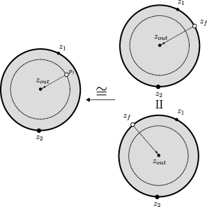
Figure 5. The diffeomorphism between $\hat{\mathcal{R}}^{1}_{2,\tau_{0}}\cup\hat{\mathcal{R}}^{1}_{2,\tau_{1}}$ and the open dense part of $\mathcal{R}^{S^{1}}_{2}$ given by $\mathcal{R}^{S^{1}_{0,1}}_{2}\cup\mathcal{R}^{S^{1}_{1,2}}_{2}$. The former spaces can in turn be compared to $\hat{\mathcal{R}}^{1}_{2}$ via cyclic permutation of labels.

By construction, this map is compatible with Floer data (this uses the fact that the Floer data on $\mathcal{R}^{S^{1}_{i,i+1}}$ agrees with the data on $\hat{\mathcal{R}}_{d}^{1}$ via the reshuffling map $\kappa^{-i}$ by (5.55)), and covers all but a codimension 1 locus in the target. Since after perturbation zero-dimensional solutions to Floer’s equation can be chosen to come from the complement of any codimension 1 locus in the source abstract moduli space, we conclude that the two operations in the Lemma, which arise from either side of (5.73), are identical up to sign. To fix the signs, note that (5.73) is in fact an oriented embedding, and all the sign twists defining the operations $\hat{\mathcal{OC}}_{d,\tau_{i}}$ are chosen to be compatible with the sign twist in the operation $\mathcal{OC}^{S^{1}}$. ∎

Next, because the Floer data used in the constructions are identical, $\hat{\mathcal{OC}}_{d,\tau_{i}}(x_{d}\otimes\cdots\otimes x_{1}):=\hat{\mathcal{OC}}_{d,\tau_{i}}(x_{d},\ldots,x_{1})$ (recall the abuse of notation $x_{i}:=[x_{i}]$) agrees with $\hat{\mathcal{OC}}(x_{i}\otimes\cdots\otimes x_{1}\otimes x_{d}\otimes\cdots\otimes x_{i+1}):=\hat{\mathcal{OC}}(x_{i},\ldots,x_{1},x_{d},\ldots,x_{i+1})$ up to a sign difference coming from orientations of abstract moduli spaces, cyclically reordering inputs, and sign twists. The following proposition computes the sign difference, and hence completes the proof of Proposition 6:

Lemma 14.

There is an equality

(5.74) $$\begin{split}\hat{\mathcal{OC}}_{d,\tau_{i}}(x_{d}\otimes\cdots\otimes x_{1})&=\hat{\mathcal{OC}}^{d}(s^{nu}(t^{i}(x_{d}\otimes\cdots x_{1})))\end{split}$$

where $s^{nu}$ is the operation (3.20) arising from changing a check term to a hat term with a sign twist.

Proof.

It is evident that $\hat{\mathcal{OC}}_{d,\tau_{i}}$ agrees with $\hat{\mathcal{OC}}_{d}\circ s^{nu}\circ t^{i}$ up to sign, as the Floer data used in the two constructions are identical. By an inductive argument it suffices to verify the following equalities of signed operations:

(5.75) $$\hat{\mathcal{OC}}_{d,\tau_{0}} =\hat{\mathcal{OC}}_{d}\circ s^{nu},$$

(5.76) $$\hat{\mathcal{OC}}_{d,\tau_{1}} =\hat{\mathcal{OC}}_{d,\tau_{0}}\circ t;$$

the remaining sign changes are entirely incremental. For the equality (5.75), we simply note that the signs appearing in the operations $\hat{\mathcal{OC}}_{d,\tau_{0}}([x_{d}],\ldots,[x_{1}])$ and $\hat{\mathcal{OC}}_{d}([x_{d}],\ldots,[x_{1}])$ differ in the following fashions:

• The abstract orientations on the moduli space of domains agree, as per Remark 46.

• The difference in sign twists is given by $\clubsuit_{d}-\hat{\star}_{d}=\sum_{i=1}^{d}|x_{i}|+|x_{d}|+d-1=(\sum_{i=1}^{d}||x_{i}||)+1+|x_{d}|=\maltese_{1}^{d}+||x_{d}||$.

All together, the parity of difference in signs is $\maltese_{1}^{d}+||x_{d}||$ which accounts for the sign in the algebraic operation $s^{nu}$ (see (3.20)); this verifies (5.75).

Next, the sign difference between the two operations in the equality (5.76) is a sum of three contributions:

• The two orientations of abstract moduli spaces from (on the slice where $z_{f}$ and $z_{out}$ are fixed; see Remark 46) $-dz_{1}\wedge\cdots\wedge dz_{d}$ to $dz_{2}\wedge\cdots\wedge dz_{d}\wedge dz_{1}$ differ by a sign change of parity

  $$d-1.$$

• For a given collection of inputs, the change in sign twisting data from $\clubsuit_{d}=\sum_{i=1}^{d}(i+1)\cdot|x_{i}|+|x_{d}|+d-1$ to $\sum_{i=1}^{d-1}(i+1)|x_{i+1}|+(d+1)|x_{1}|+|x_{1}|+d-1=\sum_{i=2}^{d}i|x_{i}|+d|x_{1}|+d-1$ ($\clubsuit_{d}$ for the sequence $(x_{2},\ldots,x_{d},x_{1})$) induces a sign change of parity

  $$\sum_{i=2}^{d}|x_{i}|+|x_{d}|+d|x_{1}|=\sum_{i=1}^{d}|x_{i}|+|x_{d}|+(d-1)|x_{1}|=\sum_{i=1}^{d}||x_{i}||+(d-1)||x_{1}||+||x_{d}||=\maltese_{1}^{d}+(d-1)||x_{1}||+||x_{d}||.$$

• Finally, the re-ordering of determinant lines of the inputs induces a sign change of parity

  $$|x_{1}|\cdot(\sum_{i=2}^{d}|x_{i}|)=||x_{1}||\cdot(\sum_{i=2}^{d}||x_{i}||)+\sum_{i=2}^{d}||x_{i}||+(d-1)||x_{1}||+(d-1)=||x_{1}||\maltese_{2}^{d}+\maltese_{1}^{d}+d||x_{1}||+(d-1)$$

The cumulative sign parity is congruent mod 2 to

$$||x_{1}||\maltese_{2}^{d}+||x_{1}||+||x_{d}||,$$

which is precisely the sign appearing in $t$ (see (3.18)). This verifies (5.76). ∎

Proof of Proposition 6.

Combine Lemmas 13 and 14 (note the definition of $B^{nu}$ given in (3.21)). ∎

5.4. Compatibility of homology-level BV operators

Before diving into the statement of chain-level equivariance, we prove a homology-level statement. The below Theorem is insufficient for studying, say, equivariant homology groups, but may be of independent interest.

Theorem 5.

The homology level open-closed map $[\mathcal{OC}]$ intertwines the Hochchild and symplectic cohomology BV operators, that is

(5.77) $$[\mathcal{OC}]\circ[B^{nu}]=[\delta_{1}]\circ[\mathcal{OC}].$$

Theorem 5 is an immediate consequence of the following chain-level statement:

Proposition 7.

The following diagram homotopy commutes:

(5.78)

where $\iota$ is the inclusion onto the left factor, which is a quasi-isomorphism by Lemma 2. More precisely, there exists an operation $\check{\mathcal{OC}}^{1}:\mathrm{CH}_{*-n}(\mathcal{F},\mathcal{F})\rightarrow CF^{*-2}(M)$ satisfying

(5.79) $$(-1)^{n+1}d\check{\mathcal{OC}}^{1}+\check{\mathcal{OC}}^{1}b=\hat{\mathcal{OC}}B^{nu}\iota-(-1)^{n}\delta_{1}\check{\mathcal{OC}}.$$

Proof of Theorem 5.

Proposition 7 immediately implies that $[\delta_{1}]\circ[\check{\mathcal{OC}}]=[\mathcal{OC}]\circ[B^{nu}]\circ[\iota]$ where $\iota:\mathrm{CH}_{*-n}(\mathcal{F},\mathcal{F})\rightarrow\mathrm{CH}_{*-n}^{nu}(\mathcal{F},\mathcal{F})$ is the inclusion of chain complexes. But by Lemma 2, $[\iota]$ is an isomorphism and by Corollary 7 $[\check{\mathcal{OC}}]=[\mathcal{OC}]$. ∎

To define $\check{\mathcal{OC}}^{1}$, consider

(5.80) $${}_{1}\check{\mathcal{R}}_{d}^{1},$$

the moduli space of discs with with $d$ positive boundary marked points $z_{1},\ldots,z_{d}$ labeled in counterclockwise order, 1 interior negative puncture $z_{out}$ equipped with an asymptotic marker, and $1$ additional interior marked point $p_{1}$ (without an asymptotic marker), marked as auxiliary. Also, with respect to the unit disc representative of any element of this moduli space fixing $z_{d}$ at $1$ and $z_{out}$ at 0 on the unit disc, $p_{1}$ should lie inside the circle of radius $\frac{1}{2}$:

(5.81) $$0<|p_{1}|<\frac{1}{2}.$$

Using the above representative, one can talk about the angle, or argument of $p_{1}$

(5.82) $$\theta_{1}:=\arg(p_{1}).$$

We require that with respect to the above representative,

(5.83) the asymptotic marker on $$z_{out} \theta_{1}$$ points in the direction .

For every representative $S\in{}_{1}\check{\mathcal{R}}_{d}^{1}$,

(5.84) $$\begin{split}&\textrm{ fix a negative cylindrical end around $z_{out}$ not containing $p_{1}$, compatible with the }\\ &\textrm{direction of the asymptotic marker, or {\it equivalently compatible with the angle $\theta_{1}$}.}\end{split}$$

We orient (5.80) as follows: pick, on a slice of the automorphism action which fixes the position of $z_{d}$ at 1 and $z_{out}$ at 0, the volume form

(5.85) $$-r_{1}dz_{1}\wedge dz_{2}\wedge\cdots\wedge dz_{d-1}\wedge dr_{1}\wedge d\theta_{1}$$

The compactification of (5.80) is a real blow-up of the ordinary Deligne-Mumford compactification, in the sense of [Kimura:1995fk] (see [Seidel:2010uq] for a first discussion in the context of Floer theory), reviewed in Appendix A.1 (note this is the case $k=1$ of the more general description therein). The result of this discussion is that the codimension 1 boundary of the compactified check moduli space ${}_{1}\overline{\check{\mathcal{R}}}_{d}^{1}$ is covered by the images of the natural inclusions of the following strata:

(5.86) $$\overline{\mathcal{R}}^{s}\times{}_{1}\overline{\check{\mathcal{R}}}_{d-s+1}^{1}$$

(5.87) $$\overline{\check{\mathcal{R}}}_{d}^{1}\times\overline{\mathcal{M}}_{1}$$

(5.88) $$\overline{\check{\mathcal{R}}}_{d}^{S^{1}}$$

The stratum (5.88) describes the locus which $|p_{1}|=\frac{1}{2}$, which is exactly the locus we defined to be the auxiliary moduli space $\mathcal{R}_{d}^{S^{1}}$ inducing the operation $\mathcal{OC}^{S^{1}}$. The strata (5.86)-(5.87) have manifold with corners structure given by standard local gluing maps using fixed choices of strip-like ends near the boundary. For (5.86) this is standard, and for (5.87), the local gluing map uses the cylindrical ends (5.84) and (4.33) (in other words, one rotates the $1$-pointed angle cylinder by an amount commensurate to the angle of the marked point $z_{d}$ on the disk before gluing; see §A.1 particularly (A.12)). See Figure 6 for a schematic of (5.80) and two out of the three types of strata (5.87)-(5.88).

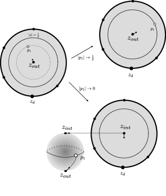
Figure 6. A schematic of an element of (5.80) on the left and a schematic of two of its three types of degenerations on the right, (5.88) (above) and (5.87) (below). The remaining type of degeneration (5.86), omitted from the figure, occurs when some boundary marked points coalesce into a disc bubble.

We will as usual fix a Floer datum for the BV homotopy, meaning an inductive choice, for every $d\geq 1$, of Floer data for every representative $S\in{}_{1}\overline{\check{\mathcal{R}}}_{d}^{1}$ varying smoothly in $S$, which on boundary strata is smoothly equivalent to a product of Floer data inductively chosen on lower dimensional moduli spaces. Such a system of choices exist again by a contractibility argument, and for any such choice, one obtains for any $d$-tuple of Lagrangians $L_{0},\ldots,L_{d-1}$, and asympotic conditions

(5.89) $$\begin{split}\vec{x}&=(x_{d},\ldots,x_{1}),\ x_{i}\in\chi(L_{i-1},L_{i\mathrm{\ mod\ }d})\\ y_{out}&\in\mathcal{O}\end{split}$$

a compactified moduli space

(5.90) $${}_{1}\overline{\check{\mathcal{R}}}_{d}^{1}(y_{out},\vec{x})$$

of maps into $M$ with source an arbitrary element $S$ of the moduli space (5.80), satisfying Floer’s equation using the Floer datum chosen for the given $S$ as in (5.4) with asymptotics and boundary conditions as in (5.5) (with the usual modifications in the Liouville case detailed in Remarks 43 and 44). The virtual dimension of every component of ${}_{1}\overline{\check{\mathcal{R}}}_{d}^{1}(y_{out},\vec{x})$ coincides (mod 2 or exactly depending on whether we are in a ${\mathbb{Z}}/2$ or ${\mathbb{Z}}$-graded setting) with

(5.91) $$\deg(y_{out})-n+d+1-\sum_{i=1}^{d}\deg(x_{i})$$

By Assumption 1, for generic choices of Floer data, the Gromov-Floer compactification of the components of virtual dimension $\leq 1$ of (5.90) are compact manifolds-with-boundary of expected dimension. For rigid elements $u$ of the moduli spaces (5.90), the orientations (5.85), and [Abouzaid:2010kx]*Lemma C.4 induce isomorphisms of orientation lines

(5.92) $$({}_{1}\check{\mathcal{R}}_{d}^{1})_{u}:o_{x_{d}}\otimes\cdots\otimes o_{x_{1}}\rightarrow o_{y}\\$$

As usual “counting rigid elements $u$,” i.e., summing application of these isomorphisms over all $u$, defines the $|o_{y_{out}}|_{\mathbf{k}}$ component of an operation $\check{\mathcal{OC}}^{1}$, up to a sign twist which we specify below:

(5.93) $$\check{\mathcal{OC}}^{1}([x_{d}],\ldots,[x_{1}]):=\sum_{u\in{}_{k}\overline{\check{\mathcal{R}}}_{d}^{1}(y_{out};\vec{x})\textrm{ rigid}}(-1)^{\check{\star}_{d}}({}_{k}\check{\mathcal{R}}_{d}^{1})_{u}([x_{d}],\ldots,[x_{1}]);\\$$

where the sign is given by

(5.94) $$\check{\star}_{d}=\deg(x_{d})+\sum_{i}i\cdot\deg(x_{i}).$$

A codimension 1 analysis of the moduli spaces (5.90) reveals:

Proposition 8.

The following equation is satisfied:

(5.95) $$(-1)^{n}\delta_{1}\check{\mathcal{OC}}+(-1)^{n}d\check{\mathcal{OC}}^{1}=\mathcal{OC}^{S^{1}}+\check{\mathcal{OC}}^{1}b$$

Proof.

The boundary of the 1-dimensional components of (5.90) are covered by the rigid components of the following types of strata:

• spaces of maps with domain lying on the codimension 1 boundary of the moduli space, i.e., in (5.86)-(5.88)

• semi-stable breakings, namely those of the form

  (5.96) $${}_{1}\overline{\check{\mathcal{R}}}_{d}^{1}(y_{1};\vec{x})\times\overline{\mathcal{M}}(y_{out};y_{1})$$

  (5.97) $$\overline{\mathcal{R}}^{1}(x;x_{i})\times{}_{1}\overline{\check{\mathcal{R}}}_{d}^{1}(y_{out};\tilde{\vec{x}})$$

  where $\tilde{\vec{x}}$ denotes the collection of inputs $\vec{x}$ with $x_{i}$ replaced with $x$.

All together, this implies, up to signs, that

(5.98) $$(-1)^{n}\delta_{1}\check{\mathcal{OC}}+(-1)^{n}d\check{\mathcal{OC}}^{1}=\mathcal{OC}^{S^{1}}+\check{\mathcal{OC}}^{1}b.$$

(5.98) is of course a shorthand for saying, for any $d$ and any tuple of $d$ cyclically composable morphisms $x_{d},\ldots,x_{1}$, that

(5.99) $$\begin{split}(-1)^{n}\sum_{i=0}^{1}\delta_{i}&\check{\mathcal{OC}}^{k-i}_{d}(x_{d},\ldots,x_{1})=\mathcal{OC}^{S^{1}}_{d}(x_{d},\ldots,x_{1})\\ &+\sum_{i,s}(-1)^{\maltese_{1}^{s}}\check{\mathcal{OC}}^{1}_{d-i+1}(x_{d},\ldots,x_{s+i+1},\mu^{i}(x_{s+i},\ldots,x_{s+1}),x_{s},\ldots,x_{1})\\ &+\sum_{i,j}(-1)^{\sharp_{j}^{i}}\check{\mathcal{OC}}^{1}_{d-i-j}(\mu^{i+j+1}(x_{i},\ldots,x_{1},x_{d},\ldots,x_{d-j}),x_{d-j-1},\ldots,x_{i+1})\end{split}$$

(recall the abuse of notation $x_{i}:=[x_{i}]$). Thus, it suffices to verify that the signs coming from the codimension 1 boundary are exactly those appearing in (5.98). (in particular, that the terms in, for instance, $\check{\mathcal{OC}}^{1}b$ appear with the right sign).

Let us recall broadly how the signs are computed. For any operator $g$ defined above such as $\mathcal{OC}$, $\mathcal{OC}^{S^{1}}$, $\mu$, $d$, $\delta_{1}$ etc., we let $g_{\mathrm{ut}}$ denote the untwisted version of the same operator, e.g., the operator whose matrix coefficients come from the induced isomorphism on orientation lines, without any sign twists by the degree of the inputs. So for instance $\mu^{d}(x_{d},\ldots,x_{1})=(-1)^{\sum_{i=1}^{d}i\deg(x_{i})}\mu^{d}_{\mathrm{ut}}(x_{d},\ldots,x_{1})$ and so on. The methods described in [Seidel:2008zr]*Prop. 12.3 and elaborated upon in [Abouzaid:2010kx]*§C.3, Lemma 5.3 and [ganatra1_arxiv]*§B, when applied to the boundary of the 1-dimensional component of the moduli space of maps, $\overline{\check{\mathcal{R}}}_{d}^{1}(y_{out},\vec{x}))$, imply the following signed equality:

(5.100) $$\begin{split}0&=d_{\mathrm{ut}}\check{\mathcal{OC}}^{1}_{\mathrm{ut}}(x_{d},\ldots,x_{1})+(\delta_{1})_{\mathrm{ut}}\check{\mathcal{OC}}_{\mathrm{ut}}(x_{d},\ldots,x_{1})\\ &-\mathcal{OC}^{S^{1}}_{\mathrm{ut}}(x_{d},\ldots,x_{1})+(-1)^{\mathfrak{f}_{d}}\check{\mathcal{OC}}^{1}b(x_{d},\ldots,x_{1})\end{split}$$

where

(5.101) $$\mathfrak{f}_{d}:=\sum_{i}(i+1)\deg(x_{i})+\deg(x_{d})=\check{\star}_{d}+\maltese_{d}-d.$$

is an auxiliary sign.

To explain this equation (5.100), we note first that the signs appearing in all terms but the last are simply induced by the boundary orientation on the moduli space of domains. The sign appearing in the first term also follows from a standard boundary orientation analysis for Floer cylinders, which we omit (but see e.g., [Seidel:2008zr]*(12.19-12.20) for a version close in spirit). The signs for the first two terms are also exactly as in Lemma 6. Finally, in the last term, the sign $(-1)^{\mathfrak{f}_{d}}\check{\mathcal{OC}}^{1}b(x_{d}\otimes\cdots\otimes x_{1})$ (compare [Seidel:2008zr]*(12.25) [ganatra1_arxiv]*(B.59)) appears as a cumulative sum of

• the sign twists which turn the untwisted operations $\check{\mathcal{OC}}^{1}_{\mathrm{ut}}$ and $\mu^{s}_{ut}$ into the usual operations $\check{\mathcal{OC}}^{1}$ and $\mu^{s}$;

• the Koszul sign appearing in the Hochschild differential $b$; and

• the boundary orientation sign appearing in the relevant (untwisted) term of $\check{\mathcal{OC}}^{1}b$, for instance $\check{\mathcal{OC}}^{1}_{\mathrm{ut}}(x_{d},\ldots,x_{n+m+1},\mu^{m}_{ut}(x_{n+m},\ldots,x_{n+1}),x_{n},\ldots,x_{1})$, which itself is as a sum of two different contributions:

  1. the comparison between the boundary (of the chosen) orientation and the product (of the chosen orientation) on the moduli of domains and

  2. Koszul reordering signs, which measure the signed failure of the method of orienting the moduli of maps (in terms of orientations of the domain and orientation lines of inputs and outputs) to be compatible with passing to boundary strata.

  See [Seidel:2008zr]*(12d) for more details in the case of the $A_{\infty}$ structure, and [Abouzaid:2010kx]*§C, [ganatra1_arxiv]*§C for the case of these computations for the open-closed map. We note in particular that the forgetful map $F_{1}:{}_{1}\check{\mathcal{R}}_{d}^{1}\rightarrow\check{\mathcal{R}}_{d}^{1}$, which forgets the point $p_{1}$ (and changes the direction of the asymptotic marker to point at $z_{d}$) has complex oriented fibers (in which just the marked point $p_{1}$ varies). So the boundary analysis of these “$\check{\mathcal{OC}^{1}}\circ b$” strata appearing here is identical to the analysis strata appearing in [Abouzaid:2010kx] and [ganatra1_arxiv] for the “$\mathcal{OC}\circ b$” strata, which is why we have not repeated it here.

Multiplying all terms of (5.100) by $(-1)^{\check{\star}_{d}+\maltese_{d}-d+1}$, and noting that, for instance, $\maltese_{d}-d+1+n-2=\deg(\check{\mathcal{OC}}^{1}(x_{d}\otimes\cdots\otimes x_{1}))$, so

(5.102) $$\begin{split}(-1)^{\check{\star}_{d}+\maltese_{d}-d+1}(\delta_{1})_{ut}\check{\mathcal{OC}}^{1}_{\mathrm{ut}}(x_{d},\ldots,x_{1})&=(-1)^{\deg(\check{\mathcal{OC}}^{1}(x_{d},\ldots,x_{1}))-n}(\delta_{1})_{ut}(-1)^{\check{\star}_{d}}\check{\mathcal{OC}}^{1}_{\mathrm{ut}}(x_{d},\ldots,x_{1})\\ &=\delta_{1}\check{\mathcal{OC}}^{1}(x_{d},\ldots,x_{1}),\end{split}$$

(and similarly for the $d\circ\mathcal{OC}^{1}$ term), it follows that

(5.103) $$\begin{split}0&=(-1)^{n}\delta_{1}\check{\mathcal{OC}}(x_{d},\ldots,x_{1})+(-1)^{n}d\check{\mathcal{OC}}^{1}(x_{d},\ldots,x_{1})\\ &-\check{\mathcal{OC}}^{1}b(x_{d},\ldots,x_{1})-(-1)^{\check{\star}_{d}+\maltese_{d}-d+1}\mathcal{OC}^{S^{1}}_{\mathrm{ut}}(x_{d},\ldots,x_{1}),\end{split}$$

but $\check{\star}_{d}+\maltese_{d}-d+1=\clubsuit_{d}$, and hence the last term above is $-\mathcal{OC}^{S^{1}}(x_{d},\ldots,x_{1})$ as desired.

∎

Proof of Proposition 7.

The “sector decomposition” performed in Proposition 6 which compares $\mathcal{OC}^{S^{1}}$ to $\hat{\mathcal{OC}}\circ B^{nu}\circ\iota$, along with Proposition 8, immediately implies the result. ∎

5.5. The main construction

We now turn to the definition of the (closed) morphism of $S^{1}$-complexes, and the proof of Theorem 1 and Corollary 1. The required data takes the form

(5.104) $$\widetilde{\mathcal{OC}}=\bigoplus_{k\geq 0}\overline{\mathbf{k}[\Lambda]/\Lambda^{2}}^{\otimes k}\otimes\mathrm{CH}_{*}^{nu}(\mathcal{F})\rightarrow CF^{*}(M)[n]$$

which is equivalent, as recalled in §2.1 to defining the collection of maps $\widetilde{\mathcal{OC}}=\{\mathcal{OC}^{k}\}_{k\geq 0}$, or $u$-linearly (see §2.3) $\widetilde{\mathcal{OC}}=\sum_{k=0}^{\infty}\mathcal{OC}^{k}u^{k}$, where

(5.105) $$\mathcal{OC}^{k}=(\check{\mathcal{OC}}^{k}+\hat{\mathcal{OC}}^{k}):=\widetilde{\mathcal{OC}}^{k|1}(\Lambda,\ldots,\Lambda,-):\mathrm{CH}_{*}^{nu}(\mathcal{F})\rightarrow CF^{*+n-2k}(M).$$

(recall from §2.1 that $\mathbf{k}[\Lambda]/\Lambda^{2}$ is our small model for $C_{-*}(S^{1})$ and $S^{1}$-complexes are by definition strictly unital $A_{\infty}$ modules over $\mathbf{k}[\Lambda]/\Lambda^{2}$). By definition, the case $k=0$ is already covered:

(5.106) $$\mathcal{OC}^{0}=(\check{\mathcal{OC}}^{0}\oplus\hat{\mathcal{OC}}^{0})=(\check{\mathcal{OC}}\oplus\hat{\mathcal{OC}})=\mathcal{OC}$$

To handle the general case ($k\geq 0$), we will associate operations to, for each $d$, compactifications of three moduli spaces of domains, in the following order:

(5.107) $${}_{k}\check{\mathcal{R}}_{d}^{1}$$

(5.108) $${}_{k}\mathcal{R}_{d}^{S^{1}}$$

(5.109) $${}_{k}\hat{\mathcal{R}}_{d}^{1};$$

The moduli space (5.108) will induce an auxiliary operation useful for the proof, whereas (5.107) and (5.109) will lead to the desired operations. For $k=0$, these moduli spaces are simply $\check{\mathcal{R}}_{d}^{1}$, $\mathcal{R}_{d}^{S^{1}}$, and $\hat{\mathcal{R}}_{d}^{1}$ as defined earlier, and the $k=1$ case of (5.107) was defined in (5.80). Inductively, we will construct, and study operations from (5.107) and (5.108) simultaneously, and then finally construct (5.109). Using these moduli spaces, we will construct the maps $\check{\mathcal{OC}}^{k}$, $\hat{\mathcal{OC}}^{k}$ and an auxiliary operation $\mathcal{OC}^{S^{1},k}$ (which we compare to $\hat{\mathcal{OC}}^{k-1}\circ B^{nu}$ in Proposition 12 below), and then prove that:

Proposition 9.

The following equations hold, for each $k\geq 0$:

(5.110) $$(-1)^{n}\sum_{i\geq 0}^{k}\delta_{i}\check{\mathcal{OC}}^{k-i} =\hat{\mathcal{OC}}^{k-1}B^{nu}+\check{\mathcal{OC}}^{k}b$$

(5.111) $$(-1)^{n}\sum_{i\geq 0}^{k}\delta_{i}\hat{\mathcal{OC}}^{k-i} =\hat{\mathcal{OC}}^{k}b^{\prime}+\check{\mathcal{OC}}^{k}(1-t).$$

All at once, denoting by $\mathcal{OC}^{k}=(\check{\mathcal{OC}}^{k}+\hat{\mathcal{OC}}^{k})$ and $\widetilde{\mathcal{OC}}=\sum_{i=0}^{\infty}\mathcal{OC}^{i}u^{i}$, $\delta_{eq}=\sum_{j=0}^{\infty}\delta_{j}^{CF}u^{j}$, and $b_{eq}=b^{nu}+uB^{nu}$ as in §2.3, we have that

(5.112) $$(-1)^{n}\delta_{eq}\circ\widetilde{\mathcal{OC}}=\widetilde{\mathcal{OC}}\circ b_{eq}.$$

This will also directly imply our main Theorems, as spelled out at the bottom of this subsection.

The space (5.107) is the moduli space of discs with with $d$ positive boundary marked points $z_{1},\ldots,z_{d}$ labeled in counterclockwise order, 1 interior negative puncture $z_{out}$ equipped with an asymptotic marker, and $k$ additional interior marked points $p_{1},\ldots,p_{k}$ (without asymptotic markers), marked as auxiliary. Also, on the unit disc representative of any element of this moduli space which fixes $z_{d}$ at $1$ and $z_{out}$ at 0, the $p_{i}$ should be strictly radially ordered with norms in $(0,\frac{1}{2})$; that is,

(5.113) $$0<|p_{1}|<\cdots<|p_{k}|<\frac{1}{2}.$$

Using the above representative, one can talk about the angle, or argument of each auxiliary interior marked point,

(5.114) $$\theta_{i}:=\arg(p_{i}).$$

We require that with respect to the above representative,

(5.115) the asymptotic marker on $$z_{out} \theta_{1} z_{d} k=0$$ points in the direction (or towards if ).

(equivalently one could define $\theta_{k+1}=0$, so that $\theta_{1}$ is always defined). See Figure 7 for a depiction.

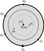
Figure 7. A representative of an element of the moduli space ${}_{3}\check{\mathcal{R}}^{1}_{5}$.

For every representative $S\in{}_{k}\check{\mathcal{R}}_{d}^{1}$,

(5.116) $$\begin{split}&\textrm{ fix a negative cylindrical end around $z_{out}$ not containing any $p_{i}$, compatible with the }\\ &\textrm{direction of the asymptotic marker, or {\it equivalently compatible with the angle $\theta_{1}$}.}\end{split}$$

The second moduli space (5.108) is the moduli space of discs with with $d$ positive boundary marked points $z_{1},\ldots,z_{d}$ labeled in counterclockwise order, 1 interior negative puncture $z_{out}$ equipped with an asymptotic marker, and $k+1$ additional interior marked points $p_{1},\ldots,p_{k},p_{k+1}$ (without asymptotic markers), marked as auxiliary. With respect to the unit disc representative of any element this moduli space fixing $z_{d}$ at $1$ and $z_{out}$ at 0, the $p_{i}$ should again be strictly radially ordered, this time with norms lying in $(0,\frac{1}{2}]$ and with $p_{k+1}$ lying on the circle of radius $\frac{1}{2}$:

(5.117) $$0<|p_{1}|<\cdots<|p_{k}|<|p_{k+1}|=\frac{1}{2}.$$

The asymptotic marker on $z_{out}$ for this representative again satisfies condition (5.115). Abstractly we have that ${}_{k}\mathcal{R}_{d}^{S^{1}}\cong\times{}_{k}\check{\mathcal{R}}_{d}^{1}\times S^{1}$, where the $S^{1}$ parameter is given by the position of $p_{k+1}$. See 8 for a depiction of ${}_{k-1}\check{\mathcal{R}}_{d}^{S^{1}}$.

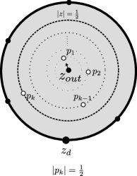
Figure 8. A representative of an element of the moduli space ${}_{k-1}\check{\mathcal{R}}_{d}^{S^{1}}$, which also arises as the boundary stratum (5.120) of ${}_{k}\overline{\check{\mathcal{R}}}_{d}^{1}$.

The compactification of (5.107) is a real blow-up of the ordinary Deligne-Mumford compactification, in the sense of [Kimura:1995fk] (see [Seidel:2010uq] for a first discussion in the context of Floer theory), reviewed in more detail in Appendix A.1. The result of the discussion there is that the codimension 1 boundary of the compactified check moduli space ${}_{k}\overline{\check{\mathcal{R}}}_{d}^{1}$ is covered by the images of the natural inclusions of the following strata:

(5.118) $$\overline{\mathcal{R}^{s}}\times{}_{k}\overline{\check{\mathcal{R}}}_{d-s+1}^{1}$$

(5.119) $${}_{s}\overline{\check{\mathcal{R}}}_{d}^{1}\times\overline{\mathcal{M}}_{k-s}$$

(5.120) $${}_{k-1}\overline{\check{\mathcal{R}}}_{d}^{S^{1}}$$

(5.121) $${}_{k}^{i,i+1}\overline{\check{\mathcal{R}}}_{d}^{1}$$

The strata (5.120)-(5.121), in which $|p_{k}|=\frac{1}{2}$ (see Figure 8) and $|p_{i}|=|p_{i+1}|$ (see Figure 9) respectively, describe the boundary loci of the ordering condition (5.113) and hence come equipped with a natural manifold with corners structure.

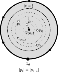
Figure 9. A representative of an element of the stratum (5.121).

The strata (5.118)-(5.119) have manifold with corners structure given by standard local gluing maps using fixed choices of strip-like ends near the boundary. For (5.118) (depicted in Figure 10) this is standard, and for (5.119) (depicted in Figure 11), the local gluing map uses the cylindrical ends (5.116) and (4.33) (in other words, one rotates the $(k-s)$-pointed angle cylinder by an amount commensurate to the angle of the first marked point $p_{k-s+1}$ on the disk before gluing) as also described in §A.1.

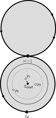
Figure 10. A representative of an element of the boundary stratum (5.118) in which a disc bubble forms (such disc bubble is allowed to include the “first” point — $z_{d}$ by our convention — but need not, and does not in the Figure).

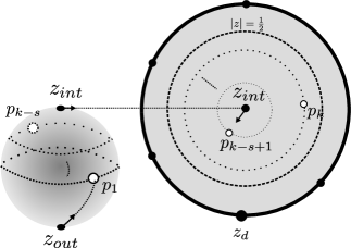
Figure 11. A representative of an element of the boundary stratum (5.119).

Associated to the stratum (5.121) where $p_{i}$ and $p_{i+1}$ have coincident magnitudes, there is a forgetful map

(5.122) $$\check{\pi}_{i}:{}_{k}^{i,i+1}\overline{\check{\mathcal{R}}}_{d}^{1}\rightarrow{}_{k-1}\overline{\check{\mathcal{R}}}_{d}^{1}$$

which simply forgets the point $p_{i+1}$. Since the norm of $p_{i+1}$ and $p_{i}$ agree on this locus, this amounts to forgetting the argument of $p_{i+1}$ (in particular, the fibers of $\check{\pi}_{i}$ are one-dimensional).

The compactification of the $S^{1}$-moduli space (5.108) can be modeled abstractly by ${}_{k}\overline{\check{\mathcal{R}}}_{d}^{1}\times S^{1}$. However, it is again preferable to give an explicit description of the boundary strata, which are covered in codimension 1 by the following strata:

(5.123) $$\overline{\mathcal{R}^{s}}\times{}_{k}\overline{\mathcal{R}}_{d-s+1}^{S^{1}}$$

(5.124) $${}_{s}\overline{\mathcal{R}}_{d}^{S^{1}}\times\overline{\mathcal{M}}_{k-s}$$

(5.125) $${}_{k}^{i,i+1}\overline{\mathcal{R}}_{d}^{S^{1}}.$$

Here, (5.123) and (5.124) are just versions of the degenerations (5.118) and (5.119), in which a collection of boundary points bubbles off, or a collection of auxiliary points convergest to $z_{out}$ and bubbles off (the fact that the latter occurs in codimension 1 is part of the “real blow-up phenomenon” already discussed). The stratum (5.125), is the locus where $|p_{i}|=|p_{i+1}|$, for $i\leq k$ (so when $i=k$, $|p_{k}|=|p_{k+1}|=\frac{1}{2}$).

As in (5.122), on the stratum (5.125) where $p_{i}$ and $p_{i+1}$ have coincident magnitudes, define the map

(5.126) $$\pi_{i}^{S^{1}}:{}_{k}^{i,i+1}\overline{\mathcal{R}}_{d}^{S^{1}}\rightarrow{}_{k-1}\overline{\mathcal{R}}_{d}^{S^{1}}$$

to be the one forgetting the point $p_{i+1}$ (so as before, this map has one-dimensional fibers).

For an element $S\in{}_{k}\overline{\mathcal{R}}_{d}^{S^{1}}$, we say that $p_{k+1}$ points at a boundary point $z_{i}$ if, for any unit disc representative of $S$ with $z_{out}$ at the origin, the ray from $z_{out}$ to $p_{k+1}$ intersects $z_{i}$. The locus where $p_{k+1}$ points at $z_{i}$ is denoted

(5.127) $${}_{k}\overline{\mathcal{R}}_{d}^{S^{1}_{i}}.$$

Similarly, we say that $p_{k+1}$ points between $z_{i}$ and $z_{i+1}$ (modulo $d$, so this includes the case of pointing between $z_{d}$ and $z_{1}$) if for such a representative, the ray from $z_{out}$ to $p_{k+1}$ intersects the portion of $\partial S$ between $z_{i}$ and $z_{i+1}$. The locus where $p_{k+1}$ points between $z_{i}$ and $z_{i+1}$ is denoted

(5.128) $${}_{k}\overline{\mathcal{R}}_{d}^{S^{1}_{i,i+1}}.$$

As before in (5.52), there is a free and properly discontinuous ${\mathbb{Z}}_{d}$-action

(5.129) $$\kappa:{}_{k}\overline{(\mathcal{R}^{1}_{d})^{S^{1}}}\rightarrow{}_{k}\overline{(\mathcal{R}^{1}_{d})^{S^{1}}}$$

which cyclically permutes the labels of the boundary marked points; as before, $\kappa$ changes the label $z_{i}$ to $z_{i+1}$ for $i<d$, and $z_{d}$ to $z_{1}$ (compare Lemma 12).

Finally, we come to the third moduli space (5.109), the moduli space of discs with with $d+1$ positive boundary marked points $z_{1},\ldots,z_{d},z_{f}$ labeled in counterclockwise order, 1 interior negative puncture $z_{out}$ equipped with an asymptotic marker, and $k$ additional interior marked points $p_{1},\ldots,p_{k}$ (without an asymptotic marker), marked as auxiliary, staisfying a strict radial ordering condition as before: for any representative element with $z_{f}$ fixed at 1 and $z_{out}$ at 0, we require (5.113) to hold, as well as condition (5.115). The boundary marked point $z_{f}$ is also marked as auxiliary, but apart from this designation we see that (identifying $z_{f}$ with $z_{d+1}$) ${}_{k}\hat{\mathcal{R}}_{d}^{1}\cong{}_{k}\check{\mathcal{R}}_{d+1}^{1}$. See Figure 12.

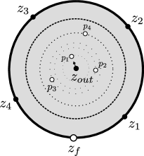
Figure 12. A representative of an element of the moduli space ${}_{4}\hat{\mathcal{R}}^{1}_{4}$.

In codimension 1, the compactification ${}_{k}\overline{\hat{\mathcal{R}}}_{d}^{1}$ has boundary covered by inclusions of the following strata:

(5.130) $$\overline{\mathcal{R}}^{s}\times{}_{k}\overline{\hat{\mathcal{R}}}_{d-s+1}^{1}$$

(5.131) $$\overline{\mathcal{R}}^{m,f_{k}}\times_{d-m+1}{}_{k}\overline{\check{\mathcal{R}}}^{1}_{d-m+1}\ \ \ 1\leq k\leq m$$

(5.132) $${}_{s}\overline{\hat{\mathcal{R}}}_{d}^{1}\times\overline{\mathcal{M}}_{k-s}$$

(5.133) $${}_{k-1}\overline{\hat{\mathcal{R}}}_{d}^{S^{1}}$$

(5.134) $${}_{k}^{i,i+1}\overline{\hat{\mathcal{R}}}_{d}^{1}$$

Once more, on strata (5.134) where $p_{i}$ and $p_{i+1}$ have coincident magnitudes (depicted in Figure 13), define the map

(5.135) $$\hat{\pi}_{i}:{}_{k}^{i,i+1}\overline{\hat{\mathcal{R}}}_{d}^{1}\rightarrow{}_{k-1}\overline{\hat{\mathcal{R}}}_{d}^{1}.$$

to be the one forgetting the point $p_{i+1}$ (so again, this map has one-dimensional fibers).

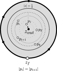
Figure 13. A representative of an element of the stratum (5.134).

On the stratum (5.133), which is the locus where $|p_{k}|=\frac{1}{2}$ (depicted in Figure 14), there is also a map of interest

(5.136) $$\hat{\pi}_{boundary}:{}_{k-1}\overline{\hat{\mathcal{R}}}_{d}^{S^{1}}\rightarrow{}_{k-1}\overline{\mathcal{R}}_{d}^{S^{1}}$$

which forgets the position of the auxiliary boundary point $z_{f}$.

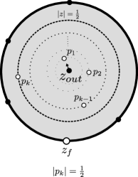
Figure 14. A representative of an element of the boundary stratum (5.133).

The stratum (5.132), depicted in Figure 15, is the locus where some subcollection of interior auxiliary points $p_{1},\ldots,p_{k-s}$ tend to zero and split off an angle-decorated cylinder (in the manner again described in §A.1 for (5.119)).

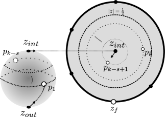
Figure 15. A representative of an element of the boundary stratum (5.132).

The strata (5.130) and (5.131) (depicted in Figures 16 and 17 respectively) are the loci where a disc bubble forms involving some boundary marked points (not including or including $z_{f}$ respectively).

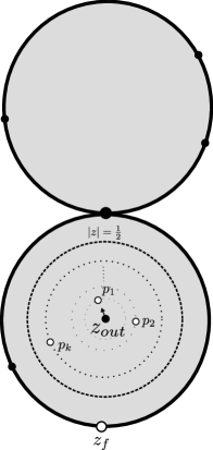
Figure 16. A representative of an element of the boundary stratum (5.130) in which a disc bubble forms not including the auxiliary point $z_{f}$.

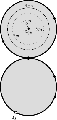
Figure 17. A representative of an element of the boundary stratum (5.131) in which a disc bubble forms including the auxiliary point $z_{f}$.

Denote by ${}_{k}{\mathcal{R}}_{d}^{1,free}:={}_{k}{\mathcal{R}}_{d}^{S^{1}_{d,1}}$ to be the sector of the moduli space ${}_{k}\mathcal{R}^{S^{1}}_{d}$ where $p_{k+1}$ points between $z_{d}$ and $z_{1}$. The auxiliary-rescaling map

(5.137) $$\pi_{f}:{}_{k}\hat{\mathcal{R}}_{d}^{1}\rightarrow{}_{k}{\mathcal{R}}_{d}^{1,free},$$

(our replacement of the “forgetful map”) can be described as follows: given a representative $S$ in ${}_{k}\hat{\mathcal{R}}_{d}^{1}$ with $z_{out}$ fixed at the origin, there is a unique point $p$ with $|p|=\frac{1}{2}$ between $z_{out}$ and $z_{f}$. $\pi_{f}(S)$ is the element of ${}_{k}\mathcal{R}^{S^{1}}_{d}$ with $p_{k+1}$ equal to this point $p$ and with $z_{f}$ deleted. Of course, $z_{f}$ is not actually forgotten, because it is determined by the position of $p_{k+1}$. In particular (5.137) is a diffeomorphism. We extend this map to a map $\overline{\pi}_{f}$ from the compactification ${}_{k}\overline{\hat{\mathcal{R}}}_{d}^{1}$ as in §5.2, by putting the auxiliary point $z_{f}$ back in, eliminating any component which is not main or secondary which has only one (non-auxiliary) boundary marked point $q$, and by labeling the positive marked point below this component by $q$.

We orient the moduli spaces (5.107)-(5.109) as follows: picking, on a slice of the automorphism action which fixes the position of $z_{d}$ at 1 and $z_{out}$ at 0, the volume forms

(5.138) $$-r_{1}\cdots r_{k}dz_{1}\wedge dz_{2}\wedge\cdots\wedge dz_{d-1}\wedge dr_{1}\wedge d\theta_{1}\wedge\cdots\wedge dr_{k}\wedge d\theta_{k}$$

(5.139) $$r_{1}\cdots r_{k}dz_{1}\wedge dz_{2}\wedge\cdots\wedge dz_{d-1}\wedge d\theta_{k+1}\wedge dr_{1}\wedge d\theta_{1}\wedge\cdots\wedge dr_{k}\wedge d\theta_{k}$$

(5.140) $$r_{1}\cdots r_{k}dz_{1}\wedge dz_{2}\wedge\cdots\wedge dz_{d-1}\wedge dz_{f}\wedge dr_{1}\wedge d\theta_{1}\wedge\cdots\wedge dr_{k}\wedge d\theta_{k}.$$

Above, $(r_{i},\theta_{i})$ denote the polar coordinate positions of the point $p_{i}$ (we could equivalently use Cartesian coordinates $(x_{i},y_{i})$ and substitute $dx_{i}\wedge dy_{i}$ for every instance of $r_{i}dr_{i}\wedge d\theta_{i}$, but polar coordinates are straightforwardly compatible with the boundary stratum where $|p_{k}|=\frac{1}{2}$).

A Floer datum on a stable disc $S$ in ${}_{k}\overline{\check{\mathcal{R}}}_{d}^{1}$ or a stable disc $S$ in ${}_{k}\overline{\mathcal{R}}_{d}^{S^{1}}$ is simply a Floer datum for $S$ in the sense of §5.1. A Floer datum on a stable disc $S\in{}_{k}\overline{\hat{\mathcal{R}}}_{d}^{1}$ is a Floer datum for $\overline{\pi}_{f}(S)$.

Again we will make a system of choices of Floer data for the above moduli spaces. A Floer datum for the cyclic open-closed map is an inductive sequence of choices, for every $k\geq 0$ and $d\geq 1$, of Floer data for every representative $S_{0}\in{}_{k}\overline{\check{\mathcal{R}}}_{d}^{1}$, $S_{1}\in{}_{k}\overline{\mathcal{R}}_{d}^{S^{1}}$, and $S_{2}\in{}_{k}\overline{\hat{\mathcal{R}}}_{d}^{1}$, varying smoothly in $S_{0}$, $S_{1}$ and $S_{2}$, which satisfies the usual consistency condition: the choice of Floer datum on any boundary stratum should agree with the previously inductively chosen datum along any boundary stratum for which (is possibly a product of moduli spaces for) we have already inductively picked data. Moreover, this choice should satisfy a series of additional requirements: First, for $S_{0}\in{}_{k}\overline{\check{\mathcal{R}}}_{d}^{1}$,

(5.141) At a boundary stratum of the form (5.121), the Floer datum for $$S_{0}$$ is

$$\textrm{equivalent to the one pulled back from ${}_{k-1}\overline{\check{\mathcal{R}}}_{d}^{1}$ via the forgetful map $\check{\pi}_{i}$}.$$

Next, for $S_{1}\in{}_{k}\overline{\mathcal{R}}_{d}^{S^{1}}$,

(5.142) On the codimension-1 loci $${}_{k}\overline{\mathcal{R}}_{d}^{S^{1}_{i}} p_{k+1} z_{i}$$, where points at , the Floer datum

should agree with the pullback by $$\tau_{i}$$ of the existing Floer datum for the

open-closed map.

(5.143) The Floer datum should be $$\kappa \kappa$$-equivariant, where is the map (5.129).

(5.144) At a boundary stratum of the form (5.125), the Floer datum for $$S_{1}$$ is

$$\textrm{conformally equivalent to the one pulled back from ${}_{k-1}\overline{\mathcal{R}}_{d}^{S^{1}}$ via the forgetful map ${\pi}_{i}^{S^{1}}$ }.$$

Finally, for $S_{2}\in{}_{k}\overline{\hat{\mathcal{R}}}_{d}^{1}$,

(5.145) The choice of Floer datum on strata containing $$\mathcal{R}^{d,f_{i}}$$ components should be

constant along fibers of the forgetful map $$\mathcal{R}^{d,f_{i}}\rightarrow\mathcal{R}^{d-1}$$.

(5.146) The Floer datum on the main component $$(S_{2})_{0} \overline{\pi}_{f}(S_{2})$$ of should coincide with the

$$\textrm{Floer datum chosen on $(S_{2})_{0}\in{}_{k}\mathcal{R}_{d}^{1,free}\subset{}_{k}\mathcal{R}_{d}^{S^{1}}$}.$$

(5.147) At a boundary stratum of the form (5.133), the Floer datum on the main component

of $$S_{2} {}_{k}\overline{\mathcal{R}}_{d}^{S^{1}}$$ is conformally equivalent to the one pulled back from via the forgetful

$$\textrm{map $\hat{\pi}_{boundary}$ }.$$

(5.148) At a boundary stratum of the form (5.134), the Floer datum for $$S_{2}$$ is conformally

$$\textrm{equivalent to the one pulled back from ${}_{k-1}\overline{\hat{\mathcal{R}}}_{d}^{1}$ via the forgetful map $\hat{\pi}_{i}$ }.$$

The above system of requirements can be split into three broad categories: the first type concerns the compatibility with forgetful maps of Floer data along the lower strata which were not previously constrained, the second type concerns the equivariance (under a free properly discontinuous action) of the Floer data on ${}_{k}\overline{\mathcal{R}}_{d}^{S^{1}}$ as well as the relationship between the Floer datum chosen here and the ones chosen on $\overline{\check{\mathcal{R}}}_{d}^{1}$ and ${}_{k}\overline{\hat{\mathcal{R}}}_{d}^{1}$.

Proposition 10.

A Floer datum for the cyclic open-closed map exists.

Proof.

Since the choices of Floer data at each stage are contractible, this follows from the straightforward verification that, for a suitably chosen inductive order on strata, the conditions satisfied by the Floer data at various strata do not contradict each other. We use the following inductive order: first, say we’ve chosen a Floer datum for the $A_{\infty}$ structure as in §3.3 along with a BV compatible Floer datum for the non-unital open-closed map following §5.3. In particular, we have chosen Floer data for the moduli spaces $\overline{\mathcal{R}}^{d,f_{i}}$ (per Appendix A.2), ${}_{0}\overline{\check{\mathcal{R}}}_{d}$, the auxiliary moduli space ${}_{0}\overline{\mathcal{R}}_{d}^{S^{1}}$ and (using the conditions above) induced a particular choice of Floer datum on ${}_{0}\overline{\hat{\mathcal{R}}}_{d}$. Next, inductively assuming we have made all choices at level $k-1$ $(k>0)$, we first choose Floer data for ${}_{k}\overline{\check{\mathcal{R}}}_{d}$ for each $d$, then ${}_{k}\overline{\mathcal{R}}_{d}^{S^{1}}$ for each $d$ (by pulling back a choice of Floer datum on the quotient by $\kappa$ in order to satisfy the equivariance condition), and finally note that a choice is fixed for ${}_{k}\overline{\hat{\mathcal{R}}}_{d}$ by the above constraints. ∎

Fixing a Floer datum for the cyclic open-closed map, we obtain, for any $d$-tuple of Lagrangians $L_{0},\ldots,L_{d-1}$, and asympotic conditions

(5.149) $$\begin{split}\vec{x}&=(x_{d},\ldots,x_{1}),\ x_{i}\in\chi(L_{i-1},L_{i\mathrm{\ mod\ }d})\\ y_{out}&\in\mathcal{O}\end{split}$$

Gromov-Floer compactified moduli spaces

(5.150) $${}_{k}\overline{\check{\mathcal{R}}}_{d}^{1}(y_{out},\vec{x})$$

(5.151) $${}_{k}\overline{\mathcal{R}}_{d}^{S^{1}}(y_{out},\vec{x})$$

(5.152) $${}_{k}\overline{\hat{\mathcal{R}}}_{d}^{1}(y_{out},\vec{x})$$

of maps into $M$ from an arbitrary element $S$ of the moduli spaces (5.107), (5.108), and (5.109) respectively (or rather from $\pi_{f}(S)$ in the case of (5.109)) satisfying Floer’s equation using the Floer datum chosen for the given $S$ as in (5.4) with asymptotics and Lagrangian boundary conditions as in (5.5) (again with the modifications as in Remarks 43 or 44 for compact or wrapped Fukaya categories of Liouville manifolds). The virtual dimension of each component of these moduli spaces coincides (mod 2 or exactly, depending on whether we are ${\mathbb{Z}}/2$ or ${\mathbb{Z}}$-graded) with

(5.153) (for $${}_{k}\overline{\check{\mathcal{R}}}_{d}^{1}(y_{out},\vec{x}) \deg(y_{out})-n+d-1-\sum_{i=1}^{d}\deg(x_{i})+2k;$$)

(5.154) (for $${}_{k}\overline{\mathcal{R}}_{d}^{S^{1}}(y_{out},\vec{x}) \deg(y_{out})-n+d-\sum_{i=1}^{d}\deg(x_{i})+2k;$$)

(5.155) (for $${}_{k}\overline{\hat{\mathcal{R}}}_{d}^{1}(y_{out},\vec{x}) \deg(y_{out})-n+d-\sum_{i=1}^{d}\deg(x_{i})+2k.$$)

By Assumption 1, for generic choices of Floer data, the Gromov-Floer compactifications of the components of virtual dimension $\leq 1$ of (5.150) - (5.152) are compact manifolds-with-boundary of the expected dimension. For rigid elements $u$ in the moduli spaces (5.150) - (5.152), (which occur for asymptotics $(y,\vec{x})$ satisfying (5.153) = 0, (5.154) = 0, or (5.155) = 0 respectively), the orientations (5.138), (5.139), (5.140) and [Abouzaid:2010kx]*Lemma C.4 induce isomorphisms of orientation lines

(5.156) $$({}_{k}\check{\mathcal{R}}_{d}^{1})_{u}:o_{x_{d}}\otimes\cdots\otimes o_{x_{1}}\rightarrow o_{y}$$

(5.157) $$({}_{k}\mathcal{R}_{d}^{S^{1}})_{u}:o_{x_{d}}\otimes\cdots\otimes o_{x_{1}}\rightarrow o_{y}$$

(5.158) $$({}_{k}\hat{\mathcal{R}}_{d}^{1})_{u}:o_{x_{d}}\otimes\cdots\otimes o_{x_{1}}\rightarrow o_{y}.$$

Summing the application of these isomorphisms over all rigid $u$ (or “counting rigid elements”) defines the $|o_{y_{out}}|_{\mathbf{k}}$ component of three families of operations $\check{\mathcal{OC}}^{k}$, ${\mathcal{OC}}^{S^{1},k}$, $\hat{\mathcal{OC}}^{k}$ up to a sign twist specified below: define

(5.159) $$\check{\mathcal{OC}}^{k}([x_{d}],\ldots,[x_{1}]) :=\sum_{u\in{}_{k}\overline{\check{\mathcal{R}}}_{d}^{1}(y_{out};\vec{x})\textrm{ rigid}}(-1)^{\check{\star}_{d}}({}_{k}\check{\mathcal{R}}_{d}^{1})_{u}([x_{d}],\ldots,[x_{1}]);$$

(5.160) $$\mathcal{OC}^{S^{1},k}([x_{d}],\ldots,[x_{1}]) :=\sum_{u\in{}_{k}\overline{\mathcal{R}}_{d}^{S^{1}}(y_{out};\vec{x})\textrm{ rigid}}(-1)^{\star_{d}^{S^{1}}}({}_{k}\mathcal{R}_{d}^{S^{1}})_{u}([x_{d}],\ldots,[x_{1}]);$$

(5.161) $$\hat{\mathcal{OC}}^{k}([x_{d}],\ldots,[x_{1}]) :=\sum_{u\in{}_{k}\overline{\hat{\mathcal{R}}}_{d}^{1}(y_{out};\vec{x})\textrm{ rigid}}(-1)^{\hat{\star}_{d}}({}_{k}\hat{\mathcal{R}}_{d}^{1})_{u}([x_{d}],\ldots,[x_{1}]).$$

where the signs are given by

(5.162) $$\check{\star}_{d} =\deg(x_{d})+\sum_{i}i\cdot\deg(x_{i}).$$

(5.163) $$\star_{d}^{S^{1}}=\clubsuit_{d} =\sum_{i=1}^{d}(i+1)\cdot\deg(x_{i})+\deg(x_{d})+d-1=\check{\star}_{d}+\maltese_{d}-1$$

(5.164) $$\hat{\star}_{d} =\sum_{i}i\cdot\deg(x_{i}).$$

A codimension 1 analysis of the moduli spaces (5.150) and (5.152) reveals:

Proposition 11.

The following equations hold for each $k\geq 0$:

(5.165) $$(-1)^{n}\sum_{i=0}^{k}\delta_{i}\check{\mathcal{OC}}^{k-i} =\mathcal{OC}^{S^{1},k-1}+\check{\mathcal{OC}}^{k}b$$

(5.166) $$(-1)^{n}\sum_{i=0}^{k}\delta_{i}\hat{\mathcal{OC}}^{k-i} =\hat{\mathcal{OC}}^{k}b^{\prime}+\check{\mathcal{OC}}^{k}(1-t).$$

Proof.

The boundary of the 1-dimensional components of (5.150) are covered by the (rigid components of) the following types of strata:

• spaces of maps with domain lying on the codimension 1 boundary of the moduli space, i.e., in (5.118)-(5.121)

• semi-stable breakings, namely those of the form

  (5.167) $${}_{k}\overline{\check{\mathcal{R}}}_{d}^{1}(y_{1};\vec{x})\times\overline{\mathcal{M}}(y_{out};y_{1})$$

  (5.168) $$\overline{\mathcal{R}}^{1}(x;x_{i})\times{}_{k}\overline{\check{\mathcal{R}}}_{d}^{1}(y_{out};\tilde{\vec{x}})$$

  where again $\tilde{\vec{x}}$ denotes the collection of inputs $\vec{x}$ with $x_{i}$ replaced with $x$.

All together, this implies, up to sign, that

(5.169) $$(-1)^{n}\sum_{i=0}^{k}\delta_{i}\check{\mathcal{OC}}^{k-i}=\mathcal{OC}^{S^{1},k-1}+\check{\mathcal{OC}}^{k}b+\sum_{i=1}^{k-1}\check{\mathcal{OC}}^{k,i,i+1},$$

where $\check{\mathcal{OC}}^{k,i,i+1}$ is an operation corresponding with some sign twist to (5.121). (5.169) is of course a shorthand for saying, for a tuple of $d$ cyclically composable morphisms $x_{d},\ldots,x_{1}$ (recalling the abuse of notation $x_{i}:=[x_{i}]$), that

(5.170) $$\begin{split}(-1)^{n}\sum_{i=0}^{k}\delta_{i}\check{\mathcal{OC}}^{k-i}_{d}(x_{d},\ldots,x_{1})&=\mathcal{OC}^{S^{1},k-1}_{d}(x_{d},\ldots,x_{1})+\sum_{i=1}^{k-1}\check{\mathcal{OC}}^{k,i,i+1}_{d}(x_{d},\ldots,x_{1})\\ &+\sum_{i,s}(-1)^{\maltese_{1}^{s}}\check{\mathcal{OC}}^{k}_{d-i+1}(x_{d},\ldots,x_{s+i+1},\mu^{i}(x_{s+i},\ldots,x_{s+1}),x_{s},\ldots,x_{1})\\ &+\sum_{i,j}(-1)^{\sharp_{j}^{i}}\check{\mathcal{OC}}^{k}(\mu^{i+j+1}(x_{i},\ldots,x_{1},x_{d},\ldots,x_{d-j}),x_{d-j-1},\ldots,x_{i+1}).\end{split}$$

We first note that in fact the operation $\check{\mathcal{OC}}^{k,i,i+1}=\sum_{d}\check{\mathcal{OC}}_{d}^{k,i,i+1}$ is zero, because by condition (5.141), the Floer datum chosen for elements $S$ in (5.121) are constant along the one-dimensional fibers of $\check{\pi}_{i}$. Hence, elements of the moduli space with source in (5.121) are never rigid (see Lemma 6 for an analogous and more detailed explanation).

Thus, it suffices to verify that the signs coming from the codimension 1 boundary are exactly those appearing in (5.169). We can safely ignore studying any signs for the vanishing operations such as $\hat{\mathcal{OC}}^{k,i,i+1}$. The remaining sign analysis is exactly as in Proposition 8; more precisely note that the forgetful map $\check{F}_{k}:{}_{k}\check{\mathcal{R}}_{d}^{1}\rightarrow{}_{1}\check{\mathcal{R}}_{d}^{1}$ which forgets $p_{1},\ldots,p_{k-1}$ has complex oriented fibers, and in particular (since the marked points $p_{i}$ contribute complex domain orientations and do not introduce any new orientation lines) the sign computations sketched in Proposition 8 carry over for any strata whose domain is pulled back from a boundary stratum of ${}_{1}\check{\mathcal{R}}_{d}^{1}$ (in turn, as described in Proposition 8, the sign computations for ${}_{1}\check{\mathcal{R}}_{d}^{1}$ largely reduce to those for ${}_{0}\check{\mathcal{R}}_{d}^{1}$. This verifies (5.169).

Similarly, for the hat moduli space, an analysis of the boundary of 1-dimensional moduli spaces of maps tells us, up to sign verification:

(5.171) $$(-1)^{n}\sum_{i=0}^{k}\delta_{i}\hat{\mathcal{OC}}^{k-i}=\hat{\mathcal{OC}}^{k}b^{\prime}+\check{\mathcal{OC}}^{k}(1-t)+\hat{\mathcal{OC}}^{k,k,k+1}+\sum_{i=1}^{k-1}\hat{\mathcal{OC}}^{k,i,i+1},$$

where $\hat{\mathcal{OC}}^{k,k,k+1}$ is an operation corresponding with some sign twist to (5.133) and $\hat{\mathcal{OC}}^{k,i,i+1}$ is an operation corresponding with some sign twist to (5.134). The conditions (5.147)-(5.148) similarly imply that $\hat{\mathcal{OC}}^{k,k,k+1}$ and $\hat{\mathcal{OC}}^{k,i,i+1}$ are zero, so it is not necessary to even establish what the signs for these terms are.

To verify signs for (5.171), we apply the principle discussed in the proof of Lemma 11, in which by treating the auxiliary boundary marked point $z_{f}$ as possessing a “formal unit element asymptotic constraint $e_{+}$,” therefore viewing $\hat{\mathcal{OC}}^{k}(x_{d}\otimes\cdots\otimes x_{1}):=\hat{\mathcal{OC}}^{k}(x_{d},\ldots,x_{1})$ formally as “$\hat{\mathcal{OC}}^{k}(e^{+}\otimes x_{d}\otimes\cdots\otimes x_{1})$” the signs for the equations (5.171) applied to strings $(x_{d}\otimes\cdots\otimes x_{1})$ of length $d$ follow from the sign computations for $\check{\mathcal{OC}}$ applied to strings $(e^{+}\otimes x_{d}\cdots\otimes\cdots x_{1})$ of length $d+1$ (we note that this analysis applies to the term $\hat{\mathcal{OC}}^{k,k,k+1}$ as well, which is the hat version of $\mathcal{OC}^{S^{1},k}$; however, the former operation happens to be zero because extra symmetries imply the moduli space controlling this operation is never rigid). ∎

Next, by decomposing the moduli space ${}_{k}\mathcal{R}_{d}^{S^{1}}$ into sectors, we can write the auxiliary operation $\mathcal{OC}^{S^{1},j}$ in terms of $\hat{\mathcal{OC}}^{j}$ and Connes’ $B$ operator:

Proposition 12.

As chain-level operations,

(5.172) $$\mathcal{OC}^{S^{1},k}=\hat{\mathcal{OC}}^{k}\circ B^{nu}.$$

Proof.

The proof directly emulates Proposition 6, and as such we will give fewer details. We begin by defining operations

(5.173) $$\hat{\mathcal{OC}}^{k}_{d,\tau_{i}}$$

associated to various “sectors” of the $k+1$st marked point $p_{k+1}$ of ${}_{k}\mathcal{R}_{d}^{S^{1}}$, for $i\in{\mathbb{Z}}/d{\mathbb{Z}}$. Once more, to gain better control of the geometry of these sectors in the compactification (when the sector size can shrink to zero), we pass to an alternate model for the compactification: define

(5.174) $${}_{k}\mathcal{R}_{d,\tau_{i}}^{1}$$

to be the abstract moduli space of discs with $d+1$ boundary punctures, $z_{1},\ldots,z_{i},z_{f},z_{i+1},\ldots,z_{d}$ arranged in counterclockwise order, one interior negative puncture $z_{out}$ with asymptotic marker, and $k$ additional interior auxiliary marked points $p_{1},\ldots,p_{k}$ which are strictly radially ordered with norms in $(0,\frac{1}{2})$ for a representative fixing $z_{0}$ at 1 and $z_{out}$ at 0:

(5.175) $$0<|p_{1}|<\ldots<|p_{k}|<\frac{1}{2}.$$

Moreover, as before,

(5.176) the asymptotic marker on $$z_{out} \theta_{1} z_{f} k=0$$ points in the direction (or towards if ).

There is a bijection

(5.177) $$\tau_{i}:{}_{k}\mathcal{R}_{d,\tau_{i}}^{1}\rightarrow{}_{k}\hat{\mathcal{R}}_{d}^{1}$$

given by cyclically permuting boundary labels, and in particular we also have an auxiliary-rescaling map as in (5.137)

(5.178) $${}_{k}\mathcal{R}_{d,\tau_{i}}^{1}\rightarrow{}_{k}\mathcal{R}_{d}^{S^{1}_{i,i+1}},$$

which, for a representative with $|z_{out}|=0$, adds a point $p_{k+1}$ on the line between $z_{out}$ and $z_{f}$ with $|p_{k+1}|=\frac{1}{2}$ and deletes $z_{f}$. We choose orientations on ${}_{k}\mathcal{R}_{d,\tau_{i}}^{1}$ to be compatible with (5.178); more concretely, for a slice fixing the positions of $z_{out}$ and $z_{d}$, consider the top form

(5.179) $$r_{1}\cdots r_{k}dz_{1}\wedge dz_{2}\wedge\cdots\wedge dz_{d-1}\wedge dz_{d}\wedge dz_{f}\wedge dr_{1}\wedge d\theta_{1}\wedge\cdots\wedge dr_{k}\wedge d\theta_{k}$$

The compactification ${}_{k}\overline{\mathcal{R}}_{d,\tau_{i}}^{1}$ is inherited from the identification (5.177); the salient point is that we treat bubbled off boundary strata containing the point $z_{f}$ as coming from $\mathcal{R}^{d,f_{i}}$, the moduli space of discs with $i$th marked point forgotten (where the $i$th marked point is $z_{f}$), constructed in Appendix A.2.

We choose as a Floer datum for ${}_{k}\overline{\mathcal{R}}_{d,\tau_{i}}^{1}$ the pulled back Floer datum from (5.177), it automatically then exists and is universal and consistent as desired. Moreover we have chosen orientations as in the case $k=0$ so that the auxiliary rescaling map (5.178) is an oriented diffeomorphism extending to a map between compactifications.

Thus, given a Lagrangian labeling $\{L_{0},\ldots,L_{d-1}\}$ and compatible asymptotics $\{x_{1},\ldots,x_{d};y_{out}\}$ we obtain a moduli space of maps satisfying Floer’s equation with the chosen boundary and asymptotics

(5.180) $${}_{k}\overline{\mathcal{R}}_{d,\tau_{i}}^{1}(y_{out};\vec{x}):={}_{k}\overline{\hat{\mathcal{R}}}_{d}^{1}(y_{out};x_{i-1},\ldots,x_{1},x_{d},\ldots,x_{i}),$$

which is (for components of virtual dimension $\leq 1$) is a manifold of dimension equal to the virtual dimension of the right hand side, which is $\deg(y_{out})-n+d-\sum_{j=1}^{d}\deg(x_{j})+2k$ (with ${\mathbb{Z}}$-gradings or mod 2 if working with ${\mathbb{Z}}/2$-gradings). The isomorphisms of orientation lines

(5.181) $$({}_{k}\mathcal{R}_{d,\tau_{i}}^{1})_{u}:o_{x_{d}}\otimes\cdots\otimes o_{x_{1}}\rightarrow o_{y_{out}}$$

induced by elements $u$ of the zero-dimensional components of (5.180) define the $|o_{y_{out}}|_{\mathbf{k}}$ component of the operation $\hat{\mathcal{OC}}^{k}_{d,\tau_{i}}$, up to the following sign twist:

(5.182) $$\begin{split}\hat{\mathcal{OC}}^{k}_{d,\tau_{i}}([x_{d}],\ldots,[x_{1}])&:=\sum_{u\in{}_{k}\overline{\hat{\mathcal{R}}}_{d,\tau_{i}}^{1}(y_{out};\vec{x})\textrm{ rigid}}(-1)^{\hat{\star}_{d}}({}_{k}{\mathcal{R}}_{d,\tau_{i}}^{1})_{u}([x_{d}],\ldots,[x_{1}]),\\ \star_{d}^{S^{1}}&=\sum_{i=1}^{d}(i+1)\cdot\deg(x_{i})+\deg(x_{d})+d-1.\end{split}$$

Now, exactly as in Lemma 13, there is a chain-level equality of signed operations

(5.183) $$\mathcal{OC}^{S^{1},k}_{d}=\sum_{i=0}^{d-1}\hat{\mathcal{OC}}^{k}_{d,\tau_{i}}.$$

We recall the geometric statement underlying this; the point is by construction there is an oriented embedding

(5.184) $$\coprod_{i}{}_{k}{\mathcal{R}}^{1}_{d,\tau_{i}}\stackrel{{\scriptstyle\coprod_{i}\pi_{f}^{i}}}{{\longrightarrow}}\coprod_{i}{}_{k}\mathcal{R}^{S^{1}_{i,i+1}}_{d}\hookrightarrow{}_{k}\mathcal{R}^{S^{1}}_{d},$$

compatible with Floer data, covering all but a codimension 1 locus in the target, and moreover all the sign twists defining the operations $\mathcal{OC}^{k}_{d,\tau_{i}}$ are chosen to be compatible with the sign twist in the operation $\mathcal{OC}^{S^{1},k}$ (this uses the fact that the Floer data on ${}_{k}\mathcal{R}^{S^{1}_{i,i+1}}$ agrees with the data on ${}_{k}\hat{\mathcal{R}}_{d}^{1}$ via the cyclic permutation map $\kappa^{-i}$ by (5.55)). After perturbation zero-dimensional solutions to Floer’s equation can be chosen to come from the complement of any codimension 1 locus in the source abstract moduli space, implying the equality (5.183).

Finally, all that remains is a sign analysis whose conclusion is that,

(5.185) $$\hat{\mathcal{OC}}^{k}_{d,\tau_{i}}=\hat{\mathcal{OC}}^{k}_{d}\circ s^{nu}\circ t^{i}$$

where $s^{nu}$ is the operation arising from changing a check term to a hat term with a sign twist (3.20). (The equality up to comparing signs is immediate, as the operations are constructed with identical Floer data and hence involve counts of identical moduli spaces). The details of this sign comparison are exactly the same as in Proposition 14, including with signs, as when orienting the moduli of maps, the additional marked points $p_{1},\ldots p_{k}$ only contribute complex orientations to the moduli spaces of domains (and no additional orientation line terms). ∎

Proof of Proposition 9.

This is an immediate corollary of the previous two propositions. ∎

We now collect all of this information to finish the proof of our main result.

Proof of Theorem 1.

The pre-morphism $\widetilde{\mathcal{OC}}\in\mathrm{Rhom}_{S^{1}}^{n}(\mathrm{CH}_{*}^{nu}(\mathcal{F}),CF^{*}(M))$, written $u$-linearly as $\sum_{i}\mathcal{OC}^{k}u^{k}$, where $\mathcal{OC}^{k}=\check{\mathcal{OC}}^{k}\oplus\hat{\mathcal{OC}}^{k}$ are as constructed above, satisfies $\partial\widetilde{\mathcal{OC}}=0$ by Prop. 9, hence $\widetilde{\mathcal{OC}}$ is closed, or an $S^{1}$-complex homomorphism, also known as an $A_{\infty}$ $C_{-*}(S^{1})$ module homomorphism (see §2.1). Note that $[\mathcal{OC}^{0}]=[\mathcal{OC}]=[\check{\mathcal{OC}}]$ where the first equality is by definition and the second is by Corollary 7, hence $\widetilde{\mathcal{OC}}$ is an enhancement of $\check{\mathcal{OC}}$ (as defined in §2.1). ∎

Proof of Corollary 1.

This is an immediate consequence of Theorem 1 and the induced homotopy-invariance properties for equivariant homology groups discussed in §2, particularly Cor. 3 and Prop. 2. ∎

5.6. Variants of the cyclic open-closed map

5.6.1. Using singular (pseudo-)cycles instead of Morse cycles

Let $M$ be Liouville or compact and admissible (in which case by our convention $\bar{M}=M$ and $\partial\bar{M}=\emptyset$), and let us consider the version of $\widetilde{\mathcal{OC}}$ with target the relative cohomology $H^{*}(\bar{M},\partial\bar{M})$ as in §4.1.2. Instead of using a $C^{2}$ small Hamiltonian to define the Floer complex computing $H^{*+n}(\bar{M},\partial\bar{M})$ (which we only did for simultaneous compatibility with the symplectic cohomology case), we can pass to a geometric cycle model for the group, and then build a version of the map $\widetilde{\mathcal{OC}}$ with such a target, which simplifies many of the constructions in the previous section (in the sense that the codimension 1 boundary strata of moduli spaces, and hence the equations satisfied by $\widetilde{\mathcal{OC}}$, are strictly a subset of the terms appearing above). As such, it will be sufficient to fix some notation for the relevant moduli spaces, and state the relevant simplified results.

We denote by

(5.186) $${}_{k}\check{\mathcal{P}}_{d}^{1}$$

(5.187) $${}_{k}\mathcal{P}_{d}^{S^{1}}$$

(5.188) $${}_{k}\hat{\mathcal{P}}_{d}^{1};$$

copies of the abstract moduli spaces (5.107)-(5.109) where the interior puncture $z_{out}$ is filled in and replaced by a marked point $\bar{z}_{out}$, without any asymptotic marker. The compactifications of these moduli spaces are exactly as before, except that the auxiliary points $p_{1},\ldots,p_{k}$ are now allowed to coincide with $\bar{z}_{out}$, without breaking off an angle-decorated cylinder / element of $\mathcal{M}_{r}$ (in the language of §4.3). In other words, the real blow-up of Deligne-Mumford compactifications at $z_{out}$ described in §A.1, which was responsible for the boundary strata containing $\mathcal{M}_{r}$ factors, no longer occurs (but all other degenerations do occur). Correspondingly the codimension-1 boundaries of compactified moduli spaces have all of the strata as before except for strata containing $\mathcal{M}_{r}$’s.

Inductively choose smoothly varying families Floer data as before on these moduli spaces of domains, satisfying all of the requirements and consistency conditions as before (except for any consistency conditions involving $\mathcal{M}_{r}$ moduli spaces, which no longer occur on the boundary). For a basis $\beta_{1},\ldots,\beta_{s}$ of smooth (pseudo)-cycles in homology $H_{*}(M)$ whose Poincaré duals $[\beta_{i}^{\vee}]$ generate the cohomology $H^{*}(\bar{M},\partial\bar{M})$, one obtains moduli spaces

(5.189) $${}_{k}\check{\mathcal{P}}_{d}^{1}(\beta_{i};\vec{x})$$

(5.190) $${}_{k}\mathcal{P}_{d}^{S^{1}}(\beta_{i},\vec{x})$$

(5.191) $${}_{k}\hat{\mathcal{P}}_{d}^{1}(\beta_{i},\vec{x});$$

of moduli spaces of maps into $M$ with source an arbitrary element of the relevant domain moduli space, satisfying Floer’s equation as before, with Lagrangian boundary and asymptotics $\vec{x}$ as before, with the additional point constraint that $\bar{z}_{out}$ lie on the cycle $\beta_{i}$. As before, standard methods ensure that 0 and 1-dimensional moduli spaces are (for generic choices of perturbation data and/or $\beta_{i}$) transversely cut out manifolds of the “right” dimension and boundary, which is all that we need.

Then, define the coefficient of $[\beta_{i}^{\vee}]\in H^{*}(\bar{M},\partial\bar{M})$ in $\check{\mathcal{OC}}^{k}(x_{d}\otimes\cdots\otimes x_{1})$ to be given by signed counts (with the same sign twists as before) of the moduli spaces (5.189); similarly for $\hat{\mathcal{OC}}^{k}$ and $\mathcal{OC}^{S^{1},k}$ using the moduli spaces (5.191) and (5.190). A simplification of the arguments already given (in which the $\delta_{k}$ operations no longer occur, but every other part of the argument carries through) implies that:

Proposition 13.

The pre-morphism $\widetilde{\mathcal{OC}}=\sum_{i=0}^{\infty}\mathcal{OC}^{k}u^{k}\in\mathrm{Rhom}_{S^{1}}^{n}(\mathrm{CH}_{*}^{nu}(\mathcal{F},\mathcal{F}),H^{*}(\bar{M},\partial\bar{M}))$ satisfies

(5.192) $$\widetilde{\mathcal{OC}}\circ b_{eq}=0,$$

where $b_{eq}=b^{nu}+uB^{nu}$. In other words, $\widetilde{\mathcal{OC}}$ is a homomorphism of $S^{1}$-complexes between $\mathrm{CH}_{*}^{nu}(\mathcal{F},\mathcal{F})$ with its strict $S^{1}$ action and $H^{*}(\bar{M},\partial\bar{M})$ with its trivial $S^{1}$ action.

As usual this model of $\widetilde{\mathcal{OC}}$ again induces maps $\widetilde{\mathcal{OC}}^{+/-/\infty}$ between homotopy orbit complexes, homotopy fixed point complexes etc.; note the relevant equivariant homology chain complexes are particularly simple for the latter $H^{*}(\bar{M},\partial\bar{M})$, seeing as there is no differential and trivial circle action (e.g., $H^{*}(\bar{M},\partial\bar{M})_{hS^{1}}=(H^{*}(\bar{M},\partial\bar{M})((u))/uH^{*}(\bar{M},\partial\bar{M})[[u]],\delta_{eq}=0)$).

5.6.2. Compact Lagrangians in non-compact manifolds

Now let us explicitly restrict to the case of $M$ a Liouville manifold, and denote by $\mathcal{F}\subset\mathcal{W}$ the full-subcategory consisting of a finite collection of compact exact Lagrangian branes contained in the compact region $\overline{M}$. By Poincaré duality we may think of the map $\mathcal{OC}$ (and its cyclic analogue, $\widetilde{\mathcal{OC}}$) with target $H^{*}(\bar{M},\partial\bar{M})$ as a pairing $\mathrm{CH}_{*}^{nu}(\mathcal{F},\mathcal{F})\otimes C^{*}(M)\to\mathbf{k}[n]$. In this case, there is a non-trivial refinement of this pairing to

(5.193) $$\mathcal{OC}_{cpct}:\mathrm{CH}_{*}(\mathcal{F})\otimes SC^{*}(M)\rightarrow\mathbf{k}[-n].$$

where $SC^{*}(M)$ is the symplectic cohomology cochain complex.

Remark 47.

The refinement (5.193) relies on extra flexibility in Floer theory for compact Lagrangians compared to non-compact Lagrangians (compare Remarks 34 and 35), first alluded to in this form in [SeidelEquivariant]. This extra flexibility allows us to define operations without outputs — and in particular study a version of the open-closed map where the interior marked point and boundary marked points are all inputs— for instance by Poincaré dually treating some boundary inputs as outputs with “negative weight”.

One way to implement such operations, using the type of Floer data discussed in Remark 35, is by allowing the sub-closed one-form $\alpha_{S}$ used in Floer theoretic perturbations to have complete freedom along boundary conditions corresponding to compact Lagrangians; in contrast along possibly non-compact Lagrangian boundary conditions, $\alpha_{S}$ is required to vanish in order to appeal to the integrated maximum principle. In particular, if we allow $\alpha_{S}$ to be non-vanishing along boundary components, Stokes’ theorem no longer implies that $\alpha_{S}$ being sub-closed implies that the total “output” weights must be greater than the total “input” weights.

Remark 48.

The existence of a map $SC^{*}(M)\to\mathrm{CH}_{*}(\mathcal{F})^{\vee}[-n]$ is well known. Namely, categories $\mathcal{C}$ with a weak proper Calabi-Yau structure of dimension $n$ (such as the Fukaya category of compact Lagrangians; see e.g., [Seidel:2008zr]*(12j), [Seidel:2010aa]*Proof of Prop. 5.1, Step 1 and [Sheridan:2016]*§2.8) come equipped with isomorphisms between the dual of Hochschild chains and Hochschild co-chains $\mathrm{CH}_{*}(\mathcal{C})^{\vee}[-n]\simeq\mathrm{CH}^{*}(\mathcal{C})$, and the existence of a map $SC^{*}(M)\to\mathrm{CH}^{*}(\mathcal{F})$ was observed in [Seidel:2002ys].

The geometric moduli spaces used to establish our main result apply verbatim in this case (with the interior marked point changed to an input, and the ordering of the auxiliary marked points $p_{1},\ldots,p_{k}$ appearing in the cyclic open-closed map reversed). In this case, the operations associated to such moduli spaces imply:

Proposition 14.

Consider $\mathrm{CH}_{*}^{nu}(\mathcal{F})\otimes SC^{*}(M)$ as an $S^{1}$-complex with its diagonal $S^{1}$ action (see Lemma 1 in §2.1), and $\mathbf{k}=\underline{\mathbf{k}}^{triv}\in S^{1}\mathrm{-mod}$ with its trivial $S^{1}$-complex structure. Then, the map from $\mathrm{CH}_{*}(\mathcal{F})\otimes SC^{*}(M)$ to $\mathbf{k}$ can be enhanced to a homomorphism of $S^{1}$-complexes

$$\widetilde{\mathcal{OC}}_{cpct}\in\mathrm{Rhom}_{S^{1}}^{n}(\mathrm{CH}_{*}^{nu}(\mathcal{F})\otimes SC^{*}(M),\mathbf{k})$$

e.g., $\widetilde{\mathcal{OC}}_{cpct}$ satisfies $\partial\widetilde{\mathcal{OC}}_{cpct}=0$. In other words, in the notation of §2.3 there exists a map $\widetilde{\mathcal{OC}}_{cpct,eq}=\sum_{i=0}^{\infty}\mathcal{OC}_{cpct,i}u^{i}:\mathrm{CH}_{*}^{nu}(\mathcal{F})\otimes SC^{*}(M)\to\mathbf{k}[[u]])$ of pure degree $n$, with $[\mathcal{OC}_{cpct,0}]=[\mathcal{OC}_{cpct}]$ such that

$$\widetilde{\mathcal{OC}}_{cpct,eq}\circ((-1)^{\deg(y)}b_{eq}(\sigma)\otimes y+\sigma\otimes\delta^{SC}_{eq}(y))=0.$$

To clarify the relevant moduli spaces used, we define the spaces

(5.194) $${}_{k}\check{\mathcal{R}}_{d,cpct}^{1}$$

(5.195) $${}_{k}\mathcal{R}_{d,cpct}^{S^{1}}$$

(5.196) $${}_{k}\hat{\mathcal{R}}_{d,cpct}^{1}$$

to be copies of the abstract moduli spaces (5.107)-(5.109) where the interior puncture $z_{out}$ is now a positive puncture (still equipped with an asymptotic marker); and all of the other inputs and auxiliary points are as before, except we’ve reversed the order of the labelings $p_{1},\ldots,p_{k}$ (for notational convenience), so the ordering constraints all now read as $0<|p_{k}|<\cdots<|p_{1}|<\frac{1}{2}$. The compactified moduli spaces have boundary strata agreeing with the boundary strata of the compactified (5.107)-(5.109), except now the $\mathcal{M}_{r}$ cylinders break “above” the ${}_{k-r}\mathcal{R}_{d,cpct}^{1}$ (equipped with $\check{}$, $\hat{}$, or $S^{1}$ decoration) discs instead of “below.” The reversal of the ordering of auxiliary marked points is designed to be compatible with the ordering of the auxiliary marked points on the $\mathcal{M}_{r}$ moduli spaces when it breaks “above” (as in $\mathcal{M}_{r}$ the label numbers of the auxiliary marked points increase from top to bottom).

Equipping these moduli spaces with perturbation data satisfying the same consistency conditions and other requirements as before, and counting solutions with sign twists as before defines the terms of the pre-morphism exactly as in the previous subsections (with identical analysis to show that, for instance, the operation corresponding to ${}_{k}\mathcal{R}_{d,cpct}^{S^{1}}$ is the operation corresponding to ${}_{k-1}\hat{\mathcal{R}}_{d,cpct}^{1}$ composed with Connes’ B operator, the boundary strata in which $|p_{i}|$ and $|p_{i+1}|$ are coincident contributes trivially, and so on).

6. Calabi-Yau structures

6.1. The proper Calabi-Yau structure on the Fukaya category

Here we review the notion of a proper Calabi-Yau structure, following Kontsevich-Soibelman [Kontsevich:2009ab], and construct proper Calabi-Yau structures on Fukaya categories of compact Lagrangians (in a compact admissible or Liouville manifold). A proper Calabi-Yau structure induces chain-level topological field theoretic operations on the Hochschild chain complex of the given category, controlled by the open moduli space of curves with marked points equipped with asymptotic markers, at least one of which is an input [Costello:2006vn, Kontsevich:2009ab]. Note that Costello’s work [Costello:2006vn] constructing field-theoretic operations has the (a priori stronger) requirement that the underlying $A_{\infty}$ category be cyclic, but in characteristic zero any proper Calabi-Yau structure determines a unique quasi-isomorphism between the underlying $A_{\infty}$ category and a cyclic $A_{\infty}$ category [Kontsevich:2009ab, Thm. 10.7]; see Remark 9 for more discussion.

We say an $A_{\infty}$ category $\mathcal{A}$ is proper (sometimes called compact) if its cohomological morphism spaces $H^{*}(\hom_{\mathcal{A}}(X,Y))$ have total finite rank over $\mathbf{k}$, for each $X,Y$. Recall that for any object $X\in\mathcal{A}$, there is an inclusion of chain complexes $\hom(X,X)\rightarrow\mathrm{CH}_{*}(\mathcal{A})$ inducing a map $[i]:H^{*}(\hom(X,X))\rightarrow\mathrm{HH}_{*}(\mathcal{A})$.

Definition 10.

Let $\mathcal{A}$ be a proper category. A chain map $tr:\mathrm{CH}_{*+n}(\mathcal{A})\rightarrow\mathbf{k}$ is called a weak proper Calabi-Yau structure, or non-degenerate trace of dimension $n$ if, for any two objects $X,Y\in\mathrm{ob\ }\mathcal{A}$, the composition

(6.1) $$H^{*}(\hom_{\mathcal{A}}(X,Y))\otimes H^{n-*}(\hom_{\mathcal{A}}(Y,X))\stackrel{{\scriptstyle[\mu^{2}_{\mathcal{A}}]}}{{\rightarrow}}H^{n}(\hom_{\mathcal{A}}(Y,Y))\stackrel{{\scriptstyle[i]}}{{\rightarrow}}\mathrm{HH}_{n}(\mathcal{A})\stackrel{{\scriptstyle[tr]}}{{\rightarrow\mathbf{k}}}$$

is a perfect pairing (this non-degeneracy property evidently only depends on the homology class $[tr]$). A chain map from the non-unital Hochschild complex $tr:\mathrm{CH}_{*+n}^{nu}(\mathcal{A})\rightarrow\mathbf{k}$ is called a weak proper Calabi-Yau structure if composition with the inclusion $\mathrm{CH}_{*+n}(\mathcal{A})\subset\mathrm{CH}_{*+n}^{nu}(\mathcal{A})$ is a weak proper Calabi-Yau structure in the sense above.

Remark 49.

In the symplectic literature, weak proper Calabi-Yau structures of dimension $n$ are sometimes defined as bimodule quasi-isomorphisms $\mathcal{A}_{\Delta}\stackrel{{\scriptstyle\sim}}{{\rightarrow}}\mathcal{A}^{\vee}[n]$, where $\mathcal{A}_{\Delta}$ denotes the diagonal bimodule and $\mathcal{A}^{\vee}$ the linear dual diagonal bimodule — see [Seidel:2008zr]*(12j) and §6.2 for brief conventions on $A_{\infty}$ bimodules (see also [Tradler:2008fk]). To explain the relationship between this definition and the one above, which has sometimes been called a weakly cyclic structure or $\infty$-inner product [Tradler:2008fk, Sheridan:2016], note that for any compact $A_{\infty}$ category $\mathcal{A}$, there are quasi-isomorphisms (with explicit chain-level models)

(6.2) $$(\mathrm{CH}_{*}(\mathcal{A}))^{\vee}=\mathrm{CH}^{*}(\mathcal{A},\mathcal{A}^{\vee})\stackrel{{\scriptstyle\sim}}{{\leftarrow}}\hom_{\mathcal{A}\!-\!\mathcal{A}}(\mathcal{A}_{\Delta},\mathcal{A}^{\vee})$$

where $\hom_{\mathcal{A}\!-\!\mathcal{A}}$ denotes morphisms in the category of $A_{\infty}$ bimodules (see e.g., [Seidel:2008cr] or [ganatra1_arxiv]). Under this correspondence, non-degenerate morphisms from $\mathrm{HH}_{*}(\mathcal{A})\rightarrow\mathbf{k}$ as defined above correspond precisely (cohomologically) to weak Calabi-Yau structures, e.g., those bimodule morphisms from $\mathcal{A}_{\Delta}$ to $\mathcal{A}^{\vee}$ which are cohomology isomorphisms.

Remember that the Hochschild chain complex of an $A_{\infty}$ category $\mathcal{A}$ comes equipped with a natural chain map to the (positive) cyclic homology chain complex, the projection to homotopy orbits (2.22)

$$pr:\mathrm{CH}_{*}^{nu}(\mathcal{A})\rightarrow\mathrm{CC}^{+}_{*}(\mathcal{A})$$

modeled on the chain level by the map that sends $\alpha\mapsto\alpha\cdot u^{0}$, for $\alpha\in\mathrm{CH}^{nu}(\mathcal{A})$ (compare (2.35)).

Definition 11 (c.f. Kontsevich-Soibelman [Kontsevich:2009ab]).

A (strong) proper Calabi-Yau structure of degree $n$ is a chain map

(6.3) $$\tilde{tr}:\mathrm{CC}^{+}_{*}(\mathcal{A})\rightarrow\mathbf{k}[-n]$$

from the (positive) cyclic homology chain complex of $\mathcal{A}$ to $\mathbf{k}$ of degree $-n$, such that the induced map $tr=\tilde{tr}\circ pr:\mathrm{CH}_{*}^{nu}(\mathcal{A})\rightarrow\mathbf{k}[-n]$ (or equivalently the composition $\check{tr}$ of $tr$ with the inclusion $\mathrm{CH}_{*}(\mathcal{A})\subset\mathrm{CH}_{*}^{nu}(\mathcal{A})$) is a weak proper Calabi-Yau structure.

Via the model for cyclic chains given as $\mathrm{CC}_{*}^{+}(\mathcal{A}):=(\mathrm{CH}_{*}^{nu}(\mathcal{A})((u))/u\mathrm{CH}_{*}^{nu}(\mathcal{A})[[u]],b+uB^{nu})$, such an element $\tilde{tr}$ takes the form

(6.4) $$\tilde{tr}:=\sum_{i=0}^{\infty}tr^{k}u^{k}$$

where

(6.5) $$tr^{k}:=(\check{tr}^{k}\oplus\hat{tr}^{k}):\mathrm{CH}_{*}^{nu}(\mathcal{A})\rightarrow\mathbf{k}[-n-2k].$$

We now complete the proof of Theorem 2 described and sketched in the Introduction: first, define the putative proper Calabi-Yau structure as the composition:

(6.6) $$\tilde{tr}:\mathrm{CC}^{+}_{*}(\mathcal{F})\stackrel{{\scriptstyle\widetilde{\mathcal{OC}}^{+}}}{{\rightarrow}}C^{*+n}(\bar{M},\partial\bar{M})\otimes_{\mathbf{k}}\mathbf{k}((u))/u\mathbf{k}[[u]]\rightarrow\mathbf{k}$$

where the last map (cohomologically) sends $PD(pt)\cdot u^{0}\in H^{2n}(\bar{M},\partial\bar{M})$ to $1$, and other elements to zero (i.e., it projects to the $u^{0}$ factor then integrates over $[M]$). Instead of using a $C^{2}$ small Hamiltonian to define the Floer complex computing $H^{*+n}(\bar{M},\partial\bar{M})$ (which we only did for simultaneous compatibility with the symplectic cohomology case), we can pass to a geometric cycle model for $\widetilde{\mathcal{OC}}^{+}$ (and therefore $\tilde{tr}$) which, as described in §5.6.1 directly maps (on the chain level) to $H^{*+n}(\bar{M},\partial\bar{M})\otimes_{\mathbf{k}}\mathbf{k}((u))/u\mathbf{k}[[u]]$. With respect to this model, the map $\tilde{tr}$ involves counts of the moduli spaces described there where the interior marked point $\bar{z}_{out}$ is unconstrained, e.g., ${}_{k}\check{\mathcal{P}}_{d}^{1}([M];\vec{x})$, ${}_{k}\hat{\mathcal{P}}_{d}^{1}([M];\vec{x})$, and ${}_{k}\mathcal{P}_{d}^{S^{1}}([M];\vec{x})$; see Figure 18.

The following well-known Lemma verifies the non-degeneracy property of the map $\tilde{tr}$:

Lemma 15 (see e.g., [Seidel:2008zr]*(12j), [Sheridan:2016]*Lemma 2.4)).

The corresponding morphism $[tr]:\mathrm{HH}_{*+n}(\mathcal{F})\rightarrow\mathbf{k}$ is a non-degenerate trace (or weak proper Calabi-Yau structure).

Sketch.

This is an immediate consequence of Poincaré duality in Lagrangian Floer cohomology, see the references cited above. As a brief sketch, note that $\check{tr}^{0}\circ\mu^{2}=\check{tr}\circ\mu^{2}:\hom(X,Y)\otimes\hom(Y,X)\rightarrow\mathbf{k}$ is chain homotopic (and hence equal in cohomology) to a chain map which counts holomorphic discs with an interior marked point satisfying an empty constraint, and two (positive) boundary asymptotics on $p$, $q$, with corresponding Lagrangian boundary on $x$ and $y$. Via a further homotopy of Floer data, one can arrange that the generators of $\hom(X,Y)$ and $\hom(Y,X)$ are in bijection (for instance if one is built out of time-1 flowlines of $H$ and one out of time-1 flowlines of $-H$), and the only such rigid discs are constant discs between $p$ and the corresponding $p^{\vee}$. ∎

Proof of Theorem 2.

The above discussion constructs $\tilde{tr}$ and Lemma 15 verifies non-degeneracy. ∎

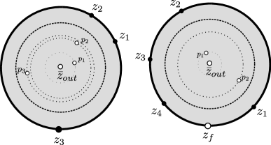
Figure 18. An image of representatives of moduli spaces ${}_{3}\check{\mathcal{P}}_{3}^{1}([M];\vec{x})$ and ${}_{2}\hat{\mathcal{P}}_{4}^{1}([M];\vec{x})$, which appear in the map $\tilde{tr}$.

6.2. The smooth Calabi-Yau structure on the Fukaya category

We give a brief overview of (a categorical version of) the notion of a (strong) smooth Calabi-Yau structure, and construct such smooth Calabi-Yau structures on (wrapped or compact) Fukaya categories under the “non-degeneracy” hypotheses of [ganatra1_arxiv]. Smooth Calabi-Yau structures were proposed in the work-in-progress [Kontsevich:uq] (see also [Kontsevich:CY]; other expositions appear e.g., in [GPS1:2015, brav_dyckerhoff_2019] — in the latter work the terminology “left” is used instead of “smooth” and “right” instead of “proper”). A smooth Calabi-Yau structure is expected (analogously to the proper case) by [Kontsevich:uq] to induce chain-level topological field theory operations on the Hochschild chain complex of the given category, controlled by the open moduli space of curves with marked points equipped with asymptotic markers, at least one of which is an output.

To state the relevant definitions, we make use of some of the theory of $A_{\infty}$ bimodules over a category $\mathcal{C}$. We do so without much explanation, instead referring readers to existing references [Seidel:2008cr, Tradler:2008fk, ganatra1_arxiv]. An $A_{\infty}$ bimodule $\mathcal{P}$ over $\mathcal{C}$ is a bilinear $A_{\infty}$ functor from $\mathcal{C}^{op}\times\mathcal{C}$ to chain complexes, which is roughly the data, of, for every pair of objects $\mathcal{C}$, a chain complex $(\mathcal{P}(X,Y),\mu^{0|1|0})$, along with ‘higher multiplication maps’ $\mu^{s|1|t}:\hom_{\mathcal{C}}({X}_{s-1},{X}_{s})\otimes\cdots\otimes\hom_{\mathcal{C}}({X}_{0},{X}_{1})\otimes\mathcal{P}(X_{0},Y_{t})\otimes\hom_{\mathcal{C}}({Y}_{t-1},{Y}_{t})\otimes\cdots\otimes\hom_{\mathcal{C}}({Y}_{0},{Y}_{1})\rightarrow\mathcal{P}(X_{s},Y_{0})$ satisfying a generalization of the $A_{\infty}$ equations. $A_{\infty}$ bimodules over $\mathcal{C}$ form a dg category $\mathcal{C}\!-\!\mathrm{mod}\!-\!\mathcal{C}$ with morphisms denoted $\hom^{*}_{\mathcal{C}\!-\!\mathcal{C}}(\mathcal{P},\mathcal{Q})$ (for dg bimodules over a dg category, this chain complex corresponds to a particular chain model for the ‘derived morphism space’ using the bar resolution). The basic examples of bimodules we require are:

• the diagonal bimodule $\mathcal{C}_{\Delta}$ which associates to a pair of objects $(K,L)$ the chain complex $\mathcal{C}_{\Delta}(K,L):=\hom_{\mathcal{C}}(L,K)$.

• for any pair of objects $A,B$, there is a Yoneda bimodule $\mathcal{Y}^{l}_{A}\otimes_{\mathbf{k}}\mathcal{Y}^{r}_{B}$ which associates to a pair of objects $(K,L)$ the chain complex $\mathcal{Y}^{l}_{A}\otimes_{\mathbf{k}}\mathcal{Y}^{r}_{B}(K,L):=\hom_{\mathcal{C}}(A,K)\otimes\hom_{\mathcal{C}}(L,B)$.

Yoneda bimodules are the analogues of the free bimodule $A\otimes A^{op}$ in the category of bimodules over an associative algebra $A$ (which are the same as $A\otimes A^{op}$ modules). Accordingly, we say a bimodule $\mathcal{P}$ is perfect if, in the category $\mathcal{C}\!-\!\mathrm{mod}\!-\!\mathcal{C}$, it is split-generated by (i.e., isomorphic to a retract of a finite complex of) Yoneda bimodules. We say that a category $\mathcal{C}$ is (homologically) smooth if $\mathcal{C}_{\Delta}$ is a perfect $\mathcal{C}$-bimodule.

Recall for what follows that for any bimodule $\mathcal{P}$ there is a cap product action

(6.7) $$\cap:\mathrm{HH}^{*}(\mathcal{C},\mathcal{P})\otimes\mathrm{HH}_{*}(\mathcal{C},\mathcal{C})\rightarrow\mathrm{HH}_{*}(\mathcal{C},\mathcal{P}),$$

and hence for any class $[\sigma]\in\mathrm{HH}_{*}(\mathcal{C},\mathcal{C})$ there is an induced map

(6.8) $$[\cap\sigma]:\mathrm{HH}^{*}(\mathcal{C},\mathcal{P})\rightarrow\mathrm{HH}_{*+\deg(\sigma)}(\mathcal{C},\mathcal{P}).$$

More generally, the cap products acts as $\mathrm{HH}^{*}(\mathcal{C},\mathcal{P})\otimes\mathrm{HH}_{*}(\mathcal{C},\mathcal{Q})\rightarrow\mathrm{HH}_{*}(\mathcal{C},\mathcal{P}\otimes_{\mathcal{C}}\mathcal{Q})$; here we are considering $\mathcal{Q}=\mathcal{C}_{\Delta}$, and then composing with the equivalence $\mathcal{P}\otimes_{\mathcal{C}}\mathcal{C}_{\Delta}\cong\mathcal{P}$. See e.g., [ganatra1_arxiv]*§2.10 for explicit chain level formulae in the variant case that $\mathcal{P}=\mathcal{C}_{\Delta}$, which can be straightforwardly adapted to the general case and then specialized to the case here.

Definition 12.

Let $\mathcal{C}$ be a homologically smooth $A_{\infty}$ category. A cycle $\sigma\in\mathrm{CH}_{-n}(\mathcal{C},\mathcal{C})$ is said to be a weak smooth Calabi-Yau structure, or a non-degenerate co-trace if, for any objects $K,L$, the operation of capping with $\sigma$ induces a homological isomorphism

(6.9) $$[\cap\sigma]:\mathrm{HH}^{*}(\mathcal{C},\mathcal{Y}^{l}_{K}\otimes_{\mathbf{k}}\mathcal{Y}^{r}_{L})\stackrel{{\scriptstyle\cong}}{{\rightarrow}}\mathrm{HH}_{*-n}(\mathcal{C},\mathcal{Y}^{l}_{K}\otimes_{\mathbf{k}}\mathcal{Y}^{r}_{L})\simeq H^{*}(\hom_{\mathcal{C}}(K,L)).$$

(this non-degeneracy property only depends on the homology class $[\sigma]$). A cycle in the non-unital Hochschild complex $\sigma\in\mathrm{CH}_{-n}^{nu}(\mathcal{C})$ is said to be a weak smooth Calabi-Yau structure if again $[\sigma]\in H^{*}(\mathrm{CH}_{-n}^{nu}(\mathcal{C}))\cong\mathrm{HH}_{-n}(\mathcal{C})$ is non-degenerate in the sense of (6.9).

Remark 50.

The second isomorphism $\mathrm{HH}_{*-n}(\mathcal{C},\mathcal{Y}^{l}_{K}\otimes_{\mathbf{k}}\mathcal{Y}^{r}_{L})\simeq H^{*}(\hom_{\mathcal{C}}(K,L))$ always holds for cohomologically unital categories (such as the Fukaya category); the content is in the first.

Remark 51.

Continuing Remark 49, there is an alternate perspective on Definition 12 using bimodules. Namely, for any bimodule $\mathcal{P}$, there is a naturally associated bimodule dual $\mathcal{P}^{!}$, defined for a pair of objects $(K,L)$ as the chain complex $\mathcal{P}^{!}(K,L):=\hom^{*}_{\mathcal{C}\!-\!\mathcal{C}}(\mathcal{P},\mathcal{Y}^{l}_{K}\otimes_{\mathbf{k}}\mathcal{Y}^{r}_{L})$. The higher bimodule structure is defined in [ganatra1_arxiv]*Def. 2.40; it is an $A_{\infty}$ analogue of defining, for an $A$ bimodule $B$, $B^{!}:=\mathrm{RHom}_{A\otimes A^{op}}(B,A\otimes A^{op})$ where $\mathrm{RHom}$ is taken with respect to the outer bimodule structure on $A\otimes A^{op}$ and the bimodule structure on $B^{!}$ comes from the inner bimodule structure; see e.g., [Ginzburg:2005aa]*§20.5.

We abbreviate $\mathcal{C}^{!}:=\mathcal{C}_{\Delta}^{!}$, and call $\mathcal{C}^{!}$ the inverse dualizing bimodule, following [Kontsevich:2009ab] (observe $H^{*}(\mathcal{C}^{!}(K,L))\cong\mathrm{HH}^{*}(\mathcal{C},\mathcal{Y}^{l}_{K}\otimes_{\mathbf{k}}\mathcal{Y}^{r}_{L})$). For a homologically smooth category $\mathcal{C}$ one notes that there is a quasi-isomorphism $\mathrm{CH}_{*-n}(\mathcal{C})\simeq\hom^{*}_{\mathcal{C}\!-\!\mathcal{C}}(\mathcal{C}_{\Delta}^{!}[n],\mathcal{C}_{\Delta})$ (see [Kontsevich:2009ab]*Rmk. 8.11 for the case of $A_{\infty}$ algebras), where the equivalence associates to any element, the bimodule morphism whose cohomology level map is the cap product operation (6.9). Non-degenerate cotraces in $\mathrm{CH}_{-n}(\mathcal{C})$ then correspond precisely then to bimodule quasi-isomorphisms $\mathcal{C}^{!}[n]\stackrel{{\scriptstyle\sim}}{{\rightarrow}}\mathcal{C}_{\Delta}$. Further discussion of these structures in the $A_{\infty}$ categorical setting will appear as part of forthcoming work with Cohen [CohenGanatra:2015].

Let $\iota:\mathrm{CC}^{-}_{*}(\mathcal{C})\rightarrow\mathrm{CH}_{*}^{nu}(\mathcal{C})$ denote the inclusion of homotopy fixed points chain map from (2.24); concretely as described in (2.36) this is the chain map sending $\sum_{i=0}^{\infty}\alpha_{i}u^{i}\mapsto\alpha_{0}$.

Definition 13.

Let $\mathcal{C}$ be a homologically smooth $A_{\infty}$ category. A (strong) smooth Calabi-Yau structure is a cycle $\tilde{\sigma}\in\mathrm{CC}^{-}_{-n}(\mathcal{C})$ such that the corresponding element $\iota(\tilde{\sigma})\in\mathrm{CH}_{-n}^{nu}(\mathcal{C})$ is a weak smooth Calabi-Yau structure.

Using these definitions and the cyclic open-closed map, we restate and prove Theorem 3. We adopt the notation of wrapped Fukaya categories in the below result, using $\mathcal{W}$ and $SC^{*}(M)$ in place of $\mathcal{F}$ and $CF^{*}(M)$ (with the understanding that for a compact symplectic manifold, these are the same).

Theorem 6 (Theorem 3 above).

Suppose a Liouville (or compact admissible symplectic) manifold is non-degenerate in the sense of [ganatra1_arxiv], meaning that the map $[\mathcal{OC}]:\mathrm{HH}_{*-n}(\mathcal{W})\rightarrow SH^{*}(M)$ hits 1. Then, the Fukaya category $\mathcal{W}$ possesses a (cohomologically) canonical geometrically defined smooth Calabi-Yau structure.

Proof.

In [ganatra1_arxiv] it was proven that, assuming non-degeneracy of $M$, the map $[\mathcal{OC}]:\mathrm{HH}_{*-n}(\mathcal{W})\rightarrow SH^{*}(M)$ is an isomorphism, $\mathcal{W}$ is homologically smooth, and moreover that the pre-image $[\sigma]$ of 1 gives a weak smooth Calabi-Yau structure in the sense described above (see [Gautogen_arxiv, GPS1:2015, GPS2:2015] for a proof of some of these facts specifically tailored to the case of compact Lagrangians in compact symplectic manifolds). Let us briefly recall how the non-degeneracy condition (6.9) is proven (which is left slightly implicit in [ganatra1_arxiv]): First, a geometric morphism of bimodules $\mathcal{CY}:\mathcal{W}_{\Delta}\to\mathcal{W}^{!}[n]$ is constructed and shown in [ganatra1_arxiv]*Thm. 1.3 to be a quasi-isomorphism under the given non-degeneracy hypotheses. Then, it is shown that capping with $[\sigma]$ is a one-sided inverse to the homological map $[\mathcal{CY}]$, and thus an isomorphism also, by the following argument: the following commutative (up to an overall sign of $(-1)^{n(n+1)/2}$) diagram is established (which can be thought of as coming from the compatibility of $\mathcal{OC}$ with module structures for Hochschild (co)homology with coefficients in $\mathcal{Y}^{l}_{K}\otimes_{\mathbf{k}}\mathcal{Y}^{r}_{L}$, and which can be extracted from the holomorphic curve theory appearing in [ganatra1_arxiv]*Thm. 13.1):

(6.10)

(here $[\mathcal{CO}_{0}]$ is the length-zero part of the closed open map for the object $L$, mapping $SH^{*}(M)$ to $H^{*}(\hom_{\mathcal{W}}(L,L))$). Plugging $[\sigma]$ into $\mathrm{HH}_{*}(\mathcal{W},\mathcal{W})$ and noting $[\mathcal{OC}]([\sigma])=1$ and $[\mu^{2}(\mathcal{CO}_{0}(1),-)]=[\mu^{2}]([e_{L}],-)$ is the identity map establishes as desired that $[\sigma\cap(\mathcal{CY}(y))]=[y]$.

To lift the weak smooth Calabi-Yau structure to a (strong) smooth Calabi-Yau structure, first we note that, because $[\mathcal{OC}]$ is an isomorphism, Corollary 1 implies that there is a commutative diagram of isomorphisms:

(6.11) $$\lx@xy@svg{\hbox{\raise 0.0pt\hbox{\kern 35.11308pt\hbox{\ignorespaces\ignorespaces\ignorespaces\hbox{\vtop{\kern 0.0pt\offinterlineskip\halign{\entry@#!@&&\entry@@#!@\cr&\\&\crcr}}}\ignorespaces{\hbox{\kern-20.32225pt\raise 0.0pt\hbox{\hbox{\kern 0.0pt\raise 0.0pt\hbox{\hbox{\kern 3.0pt\raise 0.0pt\hbox{$\textstyle{\mathrm{HC}^{-}_{*-n}(\mathcal{W})\ignorespaces\ignorespaces\ignorespaces\ignorespaces\ignorespaces\ignorespaces\ignorespaces\ignorespaces}$}}}}}}}\ignorespaces\ignorespaces\ignorespaces\ignorespaces{}{\hbox{\lx@xy@droprule}}\ignorespaces\ignorespaces\ignorespaces{\hbox{\kern 35.14423pt\raise-6.5pt\hbox{{}\hbox{\kern 0.0pt\raise 0.0pt\hbox{\hbox{\kern 3.0pt\hbox{\hbox{\kern 0.0pt\raise-1.75pt\hbox{$\scriptstyle{[\iota]}$}}}\kern 3.0pt}}}}}}\ignorespaces{\hbox{\kern 59.11308pt\raise 0.0pt\hbox{\hbox{\kern 0.0pt\raise 0.0pt\hbox{\lx@xy@tip{1}\lx@xy@tip{-1}}}}}}{\hbox{\lx@xy@droprule}}{\hbox{\lx@xy@droprule}}\ignorespaces\ignorespaces\ignorespaces\ignorespaces{}{\hbox{\lx@xy@droprule}}\ignorespaces\ignorespaces\ignorespaces{\hbox{\kern-16.77779pt\raise-20.74193pt\hbox{{}\hbox{\kern 0.0pt\raise 0.0pt\hbox{\hbox{\kern 3.0pt\hbox{\hbox{\kern 0.0pt\raise-3.16667pt\hbox{$\scriptstyle{[\widetilde{\mathcal{OC}}^{-}]}$}}}\kern 3.0pt}}}}}}\ignorespaces{\hbox{\kern 0.0pt\raise-28.55498pt\hbox{\hbox{\kern 0.0pt\raise 0.0pt\hbox{\lx@xy@tip{1}\lx@xy@tip{-1}}}}}}{\hbox{\lx@xy@droprule}}{\hbox{\lx@xy@droprule}}{\hbox{\kern 59.11308pt\raise 0.0pt\hbox{\hbox{\kern 0.0pt\raise 0.0pt\hbox{\hbox{\kern 3.0pt\raise 0.0pt\hbox{$\textstyle{\mathrm{HH}_{*-n}(\mathcal{W})\ignorespaces\ignorespaces\ignorespaces\ignorespaces}$}}}}}}}\ignorespaces\ignorespaces\ignorespaces\ignorespaces{}{\hbox{\lx@xy@droprule}}\ignorespaces\ignorespaces\ignorespaces{\hbox{\kern 82.65489pt\raise-20.74193pt\hbox{{}\hbox{\kern 0.0pt\raise 0.0pt\hbox{\hbox{\kern 3.0pt\hbox{\hbox{\kern 0.0pt\raise-1.75pt\hbox{$\scriptstyle{[\mathcal{OC}]}$}}}\kern 3.0pt}}}}}}\ignorespaces{\hbox{\kern 82.65489pt\raise-30.34776pt\hbox{\hbox{\kern 0.0pt\raise 0.0pt\hbox{\lx@xy@tip{1}\lx@xy@tip{-1}}}}}}{\hbox{\lx@xy@droprule}}{\hbox{\lx@xy@droprule}}{\hbox{\kern-35.11308pt\raise-41.48386pt\hbox{\hbox{\kern 0.0pt\raise 0.0pt\hbox{\hbox{\kern 3.0pt\raise 0.0pt\hbox{$\textstyle{H^{*}(SC^{*}(M)^{hS^{1}})\ignorespaces\ignorespaces\ignorespaces\ignorespaces}$}}}}}}}\ignorespaces\ignorespaces\ignorespaces\ignorespaces{}{\hbox{\lx@xy@droprule}}\ignorespaces\ignorespaces\ignorespaces{\hbox{\kern 35.14423pt\raise-47.98386pt\hbox{{}\hbox{\kern 0.0pt\raise 0.0pt\hbox{\hbox{\kern 3.0pt\hbox{\hbox{\kern 0.0pt\raise-1.75pt\hbox{$\scriptstyle{[\iota]}$}}}\kern 3.0pt}}}}}}\ignorespaces{\hbox{\kern 61.05353pt\raise-41.48386pt\hbox{\hbox{\kern 0.0pt\raise 0.0pt\hbox{\lx@xy@tip{1}\lx@xy@tip{-1}}}}}}{\hbox{\lx@xy@droprule}}{\hbox{\lx@xy@droprule}}{\hbox{\kern 61.05353pt\raise-41.48386pt\hbox{\hbox{\kern 0.0pt\raise 0.0pt\hbox{\hbox{\kern 3.0pt\raise 0.0pt\hbox{$\textstyle{SH^{*}(M)}$}}}}}}}\ignorespaces}}}}\ignorespaces, \textstyle{\mathrm{HC}^{-}_{*-n}(\mathcal{W})\ignorespaces\ignorespaces\ignorespaces\ignorespaces\ignorespaces\ignorespaces\ignorespaces\ignorespaces} \scriptstyle{[\iota]} \scriptstyle{[\widetilde{\mathcal{OC}}^{-}]} \textstyle{\mathrm{HH}_{*-n}(\mathcal{W})\ignorespaces\ignorespaces\ignorespaces\ignorespaces} \scriptstyle{[\mathcal{OC}]} \textstyle{H^{*}(SC^{*}(M)^{hS^{1}})\ignorespaces\ignorespaces\ignorespaces\ignorespaces} \scriptstyle{[\iota]} \textstyle{SH^{*}(M)} \textstyle{\mathrm{HC}^{-}_{*-n}(\mathcal{W})\ignorespaces\ignorespaces\ignorespaces\ignorespaces\ignorespaces\ignorespaces\ignorespaces\ignorespaces} \scriptstyle{[\iota]} \scriptstyle{[\widetilde{\mathcal{OC}}^{-}]} \textstyle{\mathrm{HH}_{*-n}(\mathcal{W})\ignorespaces\ignorespaces\ignorespaces\ignorespaces} \scriptstyle{[\mathcal{OC}]} \textstyle{H^{*}(SC^{*}(M)^{hS^{1}})\ignorespaces\ignorespaces\ignorespaces\ignorespaces} \scriptstyle{[\iota]} \textstyle{SH^{*}(M)}$$

where the horizontal maps $\iota$ are the inclusion of homotopy fixed points maps $\iota:P^{hS^{1}}\rightarrow P$ defined for any $S^{1}$-complex $P$, sending $\sum_{i=0}^{\infty}\alpha_{i}u^{i}\mapsto\alpha_{0}$.

In §4.4, and specifically (4.68), it was shown that there is a canonical geometrically defined element $\tilde{1}\in H^{*}(SC^{*}(M)^{hS^{1}})$ lifting the unit $1\in SH^{*}(M)$— essentially this is because the map $1$ is in the image of the map $H^{*}(M)\to SH^{*}(M)$, which on the chain level (as this map comes from “the inclusion of constant loops into the free loop space” and “constant loops are acted on by $S^{1}$ trivially”) can be canonically lifted to a map $C^{*}(M)\to C^{*}(M)^{hS^{1}}=C^{*}(M)[[u]]\to SC^{*}(M)^{hS^{1}}$.

Since $[\widetilde{\mathcal{OC}}^{-}]$ is an isomorphism, it follows that there is a unique (cohomological) element $[\widetilde{\sigma}]\in\mathrm{HC}^{-}_{*-n}(\mathcal{W})$ hitting $\tilde{1}$ via $[\widetilde{\mathcal{OC}}]$. By (6.11), $[\iota]([\widetilde{\sigma}])]=[\sigma]$, establishing that (any cycle representing) $[\widetilde{\sigma}]$ is a smooth Calabi-Yau structure. ∎

Appendix A Moduli spaces and operations

A.1. A real blow-up of Deligne-Mumford space

We review, in a special case, the compactifications of moduli spaces of surfaces where some interior marked points are equipped with asymptotic markers, which are a real blow-up of Deligne-Mumford moduli space as constructed in [Kimura:1995fk]. In particular, we show how boundary strata of the abstract compactifications in the sense of [Kimura:1995fk] can be identified with the specific models of the moduli spaces we use in Section 5 (the appearance of the compactifications [Kimura:1995fk] in Floer theory are not new, see e.g., [Seidel:2010uq]).

To begin, let

(A.1) $$\mathcal{M}_{2,0}$$

denote the space of spheres with $2$ marked points $z_{1},z_{2}$ removed and asymptotic markers $\tau_{1}$, $\tau_{2}$ around the $z_{1}$ and $z_{2}$, modulo automorphism. Fixing the position of $z_{1}$ and $z_{2}$ and one of $\tau_{1}$ or $\tau_{2}$ gives a diffeomorphism

$$\mathcal{M}_{2,0}\cong S^{1}.$$

On an arbitrary representative in $\mathcal{M}_{2,0}$, we can think of the map to $S^{1}$ as coming from the difference in angles between $\tau_{1}$ and $\tau_{2}$ (after, say, parallel transporting one tangent space to the other along a geodesic path).

It is convenient to parametrize this difference by a point on the sphere itself, in the following manner (though this will break symmetry between $z_{1}$ and $z_{2}$). Let

(A.2) $$\mathcal{M}_{2,1}$$

be the space of spheres with $2$ marked points $z_{1},z_{2}$ removed, an extra marked point $p$ and asymptotic markers $\tau_{1}$, $\tau_{2}$ around the $z_{1}$ and $z_{2}$, modulo automorphism such that, for any representative with position of $z_{1}$, $z_{2}$, and $p$ fixed, $\tau_{2}$ is pointing towards $p$. The remaining freedom in $\tau_{1}$ once more gives a diffeomorphism $\mathcal{M}_{2,1}\cong S^{1}$.

We can take a different representative for elements of $\mathcal{M}_{2,1}$: up to biholomorphism any element of (A.2) is equal to a cylinder sending $z_{1}$ to $+\infty$, $z_{2}$ to $-\infty$) with fixed asymptotic direction around $+\infty$ and an extra marked point $p$ at fixed height freely varying around $S^{1}$, such that the asymptotic marker at $-\infty$ coincides with the $S^{1}$ coordinate of $p$. Thus, we obtain an identification

(A.3) $$\mathcal{M}_{2,1}\cong\mathcal{M}_{1}$$

where $\mathcal{M}_{1}$ is the space in Definition 8 (with $p_{1}$ corresponding to $p$ here).

Denote by

(A.4) $${}_{k}\mathcal{R}_{d}^{1}$$

the moduli space of discs $(S,z_{1},\ldots,z_{d},z_{out},\tau_{z_{out}},p_{1},\ldots,p_{k})$ with $d$ boundary marked points $z_{1},\ldots,z_{d}$ arranged in counterclockwise order, an interior marked point with asymptotic marker $(z_{out},\tau_{z_{out}})$, and interior marked points with no asymptotic markers $p_{1},\ldots,p_{k}$ satisfying two constraints to be described below, modulo automorphism. Up to automorphism, every equivalence class of the unconstrained moduli space of such $(S,z_{1},\ldots,z_{d},z_{out},\tau_{z_{out}},p_{1},\ldots,p_{k})$ admits a unique unit disc representative with $z_{d}$ fixed at $1$ and $z_{out}$ at 0; call this the $(z_{d},z_{out})$ standard representative (or simply the standard representative). The positions of the asymptotic marker, remaining marked points, and interior marked points identify this unconstrained moduli space with an open subset of $S^{1}\times{\mathbb{R}}^{2k}\times{\mathbb{R}}^{d}$. With respect to this identification, the space (A.4) consists of those discs satisfying the following (open) “ordering constraint” on the positions of the interior marked points:

(A.5) $$\textrm{On the standard representative, }0<|p_{1}|<|p_{2}|<\cdots<|p_{k}|<\frac{1}{2}$$

along with a (codimension 1) condition on the asymptotic marker:

(A.6) $$\textrm{On the standard representative, $\tau_{z_{out}}$ points at $p_{1}$}.$$

The condition (A.5), which cuts out a manifold with corners of the larger space in which the $p_{i}$ are unconstrained, is technically convenient, as it reduces the types of bubbles that can occur with $z_{out}$). The compactification of interest, denoted

(A.7) $${}_{k}\overline{\mathcal{R}}_{d}^{1}$$

differs from the Deligne-Mumford compactification in a couple respects: firstly, we allow points $p_{i}$ and $p_{i+1}$ to be coincident without bubbling off (alternatively, we can Deligne-Mumford compactify and collapse the relevant strata).

More interestingly, (A.7) is a real blow-up of the usual Deligne-Mumford compactification along any strata in which $z_{out}$ and $p_{i}$ points bubble off (as in [Kimura:1995fk]). We will proceed to describe the codimension-1 boundary strata of (A.7) along with (after identification with the moduli spaces we introduce in this paper) the boundary chart gluing maps. Let $\Sigma=S_{0}\cup_{z_{int}^{+}=z_{int}^{-}}S_{1}$ denote a nodal surface, where

• $S_{0}$ is a sphere containing interior marked points $(z_{out},\tau_{z_{out}})$, $p_{1},\ldots,p_{j}$, and another marked point $z_{int}^{+}$, and

• $S_{1}$ is a disc with $d$ boundary marked points $z_{1},\ldots,z_{d}$, and interior marked points $z_{int}^{-}$, $p_{j+1}$, …, $p_{k}$.

To occur as a possible degenerate limit of (A.4), the relevant points $p_{i}$ on $S_{0}$ and $S_{1}$ must satisfy an ordering condition:

(A.8) For any biholomorphic $$S_{0}^{\prime} S_{0} z_{out} z_{int}^{+}$$ to with and at opposite poles,

$$\textrm{$0<|p_{1}|<\cdots<|p_{j}|<|z_{int}^{+}|$, where $|p|$ denotes the geodesic distance from $z_{out}$ to $p$ on $S_{0}^{\prime}$}.$$

(A.9) $$\textrm{For the $(z_{d},z_{int}^{-})$ standard representative of $S_{1}$, $0<|p_{j+1}|<\cdots<|p_{k}|<\frac{1}{2}$}.$$

Also,

(A.10) $$\textrm{For $S_{0}^{\prime}$ as in \eqref{orderingappa1}, the asymptotic marker $\tau_{z_{out}}$ should point (geodesically) towards $p_{1}$}.$$

The relevant codimension-1 stratum of (A.7) consists of all (automorphism classes of) such broken configurations $S_{0}\cup_{z_{int}^{+}=z_{int}^{-}}S_{1}$ as above equipped additionally with a gluing angle at the node, which is a real positive line $\tau_{z_{int}^{+},z_{int}^{-}}$ in $T_{z_{int}^{+}}S_{0}\otimes T_{z_{int}^{-}}S_{1}$, or equivalently, a pair of asymptotic markers $(\tau_{z_{int}^{+}},\tau_{z_{int}^{-}})$ around each of $z_{int}^{+}$ and $z_{int}^{-}$, modulo the diagonal $S^{1}$ rotation action. Note that the set of gluing angles (which is allowed to vary) is $S^{1}$, making this stratum codimenion-1 (the corresponding stratum in Deligne-Mumford space does not have gluing angles, and hence has real codimension 2). The gluing map takes, for a fixed pair of cylindrical ends around $z_{int}^{+}$ and $z_{int}^{-}$ compatible with the pair of asymptotic markers in the sense of (5.3), the usual gluing with respect to the chosen cylindrical ends. Note first that for a given gluing parameter, if the cylindrical ends are chosen to simply rotate as $(\tau_{z_{int}^{+}},\tau_{z_{int}^{-}})$ vary, the result of gluing after rotating $\tau_{z_{int}^{+}}$ by $\theta_{1}$ and $\tau_{z_{int}^{-}}$ by $\theta_{2}$ differs from the initial gluing by a rotation of the bottom component by $\theta_{2}-\theta_{1}$. In particular, the glued surface only indeed depends on the gluing angle associated to $(\tau_{z_{int}^{+}},\tau_{z_{int}^{-}})$ i.e., is unchanged by simultaneously rotating $(\tau_{z_{int}^{+}},\tau_{z_{int}^{-}})$.

We can recast this stratum by taking a slice of the quotient by the diagonal $S^{1}$ action appearing in the definition of gluing angle: First, note that $z_{int}^{-}$ on $S_{1}$ possesses a canonical asymptotic marker $(\tau_{z_{int}}^{-})_{canon}$ which (on the standard representative) points towards $p_{j+1}$ (our convention is that $p_{s+1}=z_{d}$ so $\tau_{z_{int}}^{-}$ points at $z_{d}$ if $j=s$). Choosing the representative $(\tau_{z_{int}^{+}},\tau_{z_{int}^{-}})$ of each gluing angle for which $\tau_{z_{int}^{-}}$ is the canonical asymptotic marker $(\tau_{z_{int}}^{-})_{canon}$, we see that the stratum described above can be identified with the space of broken configurations $S_{0}\cup_{z_{int}^{+}=z_{int}^{-}}S_{1}$ (up to automorphism) of the form:

• $S_{1}$ is as above (i.e., satisfies (A.9)) but additionally equipped with $(\tau_{z_{int}}^{-})_{canon}$, i.e., $S_{1}\in{}_{k-j}\mathcal{R}^{d}_{1}$; and

• $S_{0}$ is equipped with interior marked points with asymptotic markers $(z_{out},\tau_{z_{out}})$, $(z_{int}^{+},\tau_{z_{int}^{+}})$ and additional marked points $p_{1},\ldots,p_{j}$ satisfying (A.8) and (A.10).

In a manner as in (A.3), the space of such $S_{0}$ up to biholomorphism is precisely $\mathcal{M}_{j}$ as in Definition 8 (i.e., given any $S_{0}$, there is a 1-dimensional space of biholomorphisms to a cylinder sending $z_{int}$ and $z_{out}$ to $\infty$ and $-\infty$ while fixing the angle of $\tau_{z_{int}^{+}}$ to $1$; any two such biholomorphisms differ by translation).

Hence, we’ve identified this stratum with

(A.11) $${}_{k-j}\mathcal{R}^{d}_{1}\times\mathcal{M}_{j}$$

which will be useful in defining the relevant pseudoholomorphic curve counts. From this perspective, the boundary chart gluing maps (defined with respect to the cylindrical ends (4.33) and (4.34) on $\mathcal{M}_{j}$ and with respect to a smoothly varying choice of cylindrical end over elements of ${}_{k-j}\mathcal{R}^{d}_{1}$ compatible with $(\tau_{z_{int}}^{-})_{canon}$) just as in (4.36), rotate the (standard representative of the) angle-decorated cylinder $S_{0}$ to match the angle of its top asymptotic marker with the angle of $(\tau_{z_{int}}^{-})_{canon}$ (which coincides with the argument of $p_{j+1}$ on the standard representative). In other words, if we denote by $\theta_{i}$ the angle of $p_{i}$ in $S_{1}$ for $j+1\leq i\leq k$ (with respect to any standard representative of $S_{1}$, with the usual convention that $\theta_{k+1}$ is the argument of $z_{d}$ on the standard representative, so in particular $\theta_{j+1}$ is well-defined even if $j=k$) and $\bar{\theta}_{s}$ the angle of $p_{s}$ in $S_{0}$ for $1\leq s\leq j$, the gluing of $S_{0}$ and $S_{1}$ for small gluing parameter has (on its standard representative) marked points $p_{1},\ldots,p_{k}$ with the following angles:

(A.12) $$(\mathrm{arg}(p_{1}),\ldots,\mathrm{arg}(p_{k}))=\left(\bar{\theta}_{1}+\theta_{j+1},\bar{\theta}_{2}+\theta_{j+1},\ldots,\bar{\theta}_{j}+\theta_{j+1},\theta_{j+1},\theta_{j+2},\ldots,\theta_{k}\right).$$

A.2. Operations with a forgotten marked point

We introduce auxiliary degenerate operations that will arise as the codimension 1 boundary of the open-closed map and equivariant structure. This subsection is a very special case of the general discussion in [ganatra1_arxiv].

Let $d\geq 2$ and $i\in\{1,\ldots,d\}$. The moduli space of discs with $d$ marked points with $i$th boundary point forgotten

(A.13) $$\mathcal{R}^{d,f_{i}}$$

is exactly the moduli space of discs $\mathcal{R}^{d}$, with $i$th boundary marked point labeled as auxiliary.

The Deligne-Mumford compactification

(A.14) $$\overline{\mathcal{R}}^{d,f_{i}}$$

is exactly the usual Deligne-Mumford compactification, along with the data of an auxiliary label at the relevant boundary marked point.

For $d>2$, the $i$-forgetful map

(A.15) $$\mathcal{F}_{d,i}:\mathcal{R}^{d,f_{i}}\rightarrow\mathcal{R}^{d-1}.$$

associates to a surface $S$ the surface obtained by putting the $i$th point back in and forgetting it. This map admits an extension to the Deligne-Mumford compactification

(A.16) $$\overline{\mathcal{F}}_{d,i}:\overline{\mathcal{R}}^{d,f_{i}}\rightarrow\overline{\mathcal{R}}^{d-1}$$

as follows: eliminate any non-main components with only one non-auxiliary marked point $p$, and label the positive marked point below this component by $p$. We say that any component not eliminated is f-stable and any component eliminated is f-semistable.

The above map is only well-defined for $d>2$. In the semi-stable case $d=2$, $\mathcal{R}^{2,f_{i}}$ is a point so one can define an ad hoc map

(A.17) $$\mathcal{F}^{ss}_{i}:\mathcal{R}^{2,f_{i}}\rightarrow pt.$$

which associates to a surface $S$ the (unstable) strip $\Sigma_{1}=(-\infty,\infty)\times[0,1]$ as follows: take the unique representative of $S$ which, after its three marked points are removed, is biholomorphic to the strip $\Sigma_{1}$ with an additional puncture $(0,0)$. Then, forget/put back in the point $(0,0)$.

Definition 14.

A forgotten Floer datum for a stable disc with $i$th point auxiliary $S\in\overline{\mathcal{R}}^{d,f_{i}}$ consists of, for every component $T$ of $S$,

• a Floer datum for $T$, if $T$ does not contain the auxiliary point,

• a Floer datum for $\mathcal{F}_{j}(T)$, if $T$ is $f$-stable and contains the auxiliary point as its $j$th input.

• A Floer datum on $\mathcal{F}^{ss}_{i}(T)$ which is translation invariant, if $T$ is f-semistable.

(by translation invariant, we mean the following: note that $\Sigma_{1}$ has a canonical ${\mathbb{R}}$-action given by linear translation in the $s$ coordinate. We require $H$, $J$, and the time-shifting map/weights to be invariant under this ${\mathbb{R}}$ action, and in particular should only depend on $t\in[0,1]$ at most).

In particular, this Floer datum should only depend on the point $\overline{\mathcal{F}}_{d,i}(S)$.

Proposition 15.

Let $i\in\{1,\ldots,d\}$ with $d>1$. Then the operation associated to $\overline{\mathcal{R}}^{d,f_{i}}$ is zero if $d>2$ and the identity operation $I(\cdot)$ (up to a sign) when $d=2$.

Sketch.

Suppose first that $d>2$, and let $u$ be any solution to Floer’s equation over the space $\mathcal{R}^{d,f_{i}}$ with domain $S$. Since the Floer data on $S$ only depends on $\mathcal{F}_{d,i}(S)$, we see that maps from $S^{\prime}$ with $S^{\prime}\in\mathcal{F}_{d,i}^{-1}(\mathcal{F}_{d,i}(S))$ also give solutions to Floer’s equation with the same asymptotics. Moreover, the fibers of the map $\mathcal{F}_{d,i}$ are one-dimensional, implying that $u$ cannot be rigid, and thus the associated operation is zero.

Now suppose that $d=2$. Then the forgetful map associates to the single point $[S]\in\mathcal{R}^{2,f_{i}}$ the unstable strip with its translation invariant Floer datum. Since non-constant solutions can never be rigid (as, by translating, one can obtain other non-constant solutions), it follows that the only solutions are constant ones, and that the resulting operation is therefore the identity. ∎