Side-Tuning: A Baseline for Network Adaptation via Additive Side Networks

Abstract

When training a neural network for a desired task, one may prefer to adapt a pre-trained network rather than starting from randomly initialized weights. Adaptation can be useful in cases when training data is scarce, when a single learner needs to perform multiple tasks, or when one wishes to encode priors in the network. The most commonly employed approaches for network adaptation are fine-tuning and using the pre-trained network as a fixed feature extractor, among others.

In this paper, we propose a straightforward alternative: side-tuning. Side-tuning adapts a pre-trained network by training a lightweight “side” network that is fused with the (unchanged) pre-trained network via summation. This simple method works as well as or better than existing solutions and it resolves some of the basic issues with fine-tuning, fixed features, and other common approaches. In particular, side-tuning is less prone to overfitting, is asymptotically consistent, and does not suffer from catastrophic forgetting in incremental learning. We demonstrate the performance of side-tuning under a diverse set of scenarios, including incremental learning (iCIFAR, iTaskonomy), reinforcement learning, imitation learning (visual navigation in Habitat), NLP question-answering (SQuAD v2), and single-task transfer learning (Taskonomy), with consistently promising results.

1 Introduction

The goal of side-tuning (and generally network adaptation) is to capitalize on a pretrained model to better learn one or more novel tasks. The side-tuning approach is straightforward: it assumes access to a given (base) model $B:\mathbb{X}\rightarrow\mathbb{Y}$ that maps the input $x$ onto some representation $y$. Side-tuning then learns a side model $S:\mathbb{X}\rightarrow\mathbb{Y}$, so that the curated representations for the target task are

$$R(x)~{}\raisebox{-0.15pt}{$\triangleq$}~{}B(x)\oplus S(x),$$

for some combining operation $\oplus$. For example, choosing $B(x)\oplus S(x)~{}\raisebox{-0.15pt}{$\triangleq$}~{}\alpha B(x)+(1-\alpha)S(x)$ (commonly called $\alpha$-blending) reduces the side-tuning approach to: fine-tuning, feature extraction, and stage-wise training, depending on $\alpha$ (Fig. 2, right). Hence those can be viewed as special cases of the side-tuning approach (Figure 1).

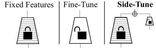
Figure 1: The side-tuning framework vs. common alternatives fine-tuning and fixed features. Given a pre-trained network that should be adapted to a new task, fine-tuning re-trains the weights in the pretrained network and fixed feature extraction trains a readout function with no re-training of the pre-trained weights. In contrast, Side-tuning adapts the pre-trained network by training a lightweight conditioned “side” network that is fused with the (unchanged) pre-trained network using summation.

Side-tuning is an example of an additive learning approach, one that adds new parameters for each new task. Since side-tuning does not change the base model, it, by design, adapts to a target task without degrading performance on the base task. Unlike many other additive approaches, side-tuning places no constraints on the structure of the base model or side network, allowing for the architecture and sizes to vary independently. In particular, while other approaches require the side network to scale with the base network, side-tuning can use tiny networks when the base only requires minor updates. By adding fewer parameters per task, side-tuning can learn more tasks before the model grows large enough to require parameter consolidation.

Substitutive methods instead opt for a single large model that is updated on each task. These methods often require adding additional constraints per-task in order to prevent inter-task interference [12, 30]. Side-tuning does not require such regularization since the base remains untouched.

Compared to existing state-of-the-art network adaptation and incremental learning approaches, we find that the more complex methods perform no better—and often worse—than side-tuning.

This straightforward mechanism deals with the key challenges of incremental learning (Sec. 4.2.1). Namely, it does not suffer from either:

• Catastrophic forgetting: tendency of a network to lose previously learned knowledge upon learning new information.

• Rigidity: Increasing inability of a network to adapt to new problems as it accrues constraints from previous problems. Note: Incremental learning literature sometimes calls this intransigence [2]. We prefer rigidity as it is clear and widely used in psychology, dating back over 70 years [27, 13].

We test side-tuning for incremental learning on iCIFAR and the more challenging iTaskonomy dataset, which we introduce, finding that incremental learning methods that work on iCIFAR often do not work as well in the more demanding setup. On these datasets, side-tuning uses side networks that are much smaller than the base. Consequently, even without consolidation, side-tuning uses fewer learnable parameters than the alternative methods.

Finally, because side-tuning treats the base model as a black-box, it can be used with non-network sources of information such as a decision trees or oracle information on a related task (see Section 4.4). Thus, side-tuning can be applied even when other model adaptation techniques cannot.

	1 Target Task		$>$ 1 Target Tasks
Method	Low Data	High Data	(incremental)
Fixed features		(Info Loss)	(Info Loss)
Fine-tuning	(Overfit)		(Forgetting)
Side-tuning

Table 1: Advantages of side-tuning vs. representative alternatives. Fixed features provide a fixed representation and if the pretrained model discarded important information then there is no way to recover the lost details. This often leads to modest performance. On the other hand, fine-tuning has a large number of learnable parameters which leads to overfitting. Side-tuning is a simple method that addresses these limitations with a small number of learnable parameters.

2 Related Work

Broadly speaking, network adaptation methods either overwrite existing parameters (substitutive methods) or freeze them and add new parameters (additive learning).

Substitutive Methods modify an existing network to solve a new task by updating some or all of the network weights (simplest approach being fine-tuning). A large body of constraint-based methods focuses on how to regularize these updates in order to prevent forgetting earlier tasks. Methods such as [30, 12, 15] impose additional constraints for each new task, which slows down learning on later tasks (see Sec. 4.2.2 on rigidity, [3]). Other methods such as [4] relegate each task to approximately orthogonal subspaces but are then unable to transfer information across tasks. Side-tuning does not require such regularization since the base remains untouched.

Additive Methods methods circumvent forgetting by freezing the weights and adding a small number of new parameters per task. One economical approach is to use off-the-shelf-features with one or more readout layers [32]. However, off-the-shelf features cannot be updated for the new task, and so recent work has focused on how features can be modulated by applying per-task learned weight masks [17, 28], by pruning [18], or by hard attention [31].

If information is missing from the original features, then recovering that information might require adding additional weights. Works such as [29, 14] introduce a new network with independent access to the input and connect to various layers from the original network. Other works like [24, 1, 25] learn task-dependent parameters (e.g. separate batch norm, linear layers) that are inserted directly into the existing network. Tying the new weights directly into the original network architecture often requires making restrictive assumptions about the original network architecture (e.g. that it must be a ResNet [8]).

Unlike these previous works, side-tuning uses only late fusion and makes no assumptions about the base network. This means it can be applied on a larger class of models. While simpler, the results suggest that side-tuning offers similar or better performance to the more complex alternatives and calls into question whether that complexity buys much in practice.

Residual Learning exploits the fact that it is often easier to approximate a difference rather than the original function. This has been successfully used in ResNets [8] where a residual is learned on top of the identity function prior. Some network adaptation methods insert new residual-modeling parameters directly into the base architecture [14, 24]. Residual learning has also been explored in robotics as residual RL [10, 33], in which we train an agent for a single task by first taking a coarse policy (e.g. behavior cloning) and then training a residual network on top (using RL). For a single task, iteratively learning residuals is known as gradient boosting, but side-tuning adds a side network to adapt a base representation for a new task. We discuss the relationship in Sec. 4.4.

Meta-learning, unlike network adaptation approaches, seeks to create networks that are inherently adaptable. Typically this proceeds by training on tasks sampled from a known task distribution. Side-tuning is fundamentally compatible with this formulation and with existing approaches (e.g. [6]). Recent work suggests that these approaches work primarily by feature adaptation rather than rapid learning [22], and feature adaptation is also the motivation for our method.

3 Side-Tuning: The Simplest Additive Approach

Side-tuning learns a side model $S(x)$ and combines it with a pre-trained base model $B(x)$. The representation for the target task is $R(x)~{}\raisebox{-0.15pt}{$\triangleq$}~{}B(x)\oplus S(x)$.

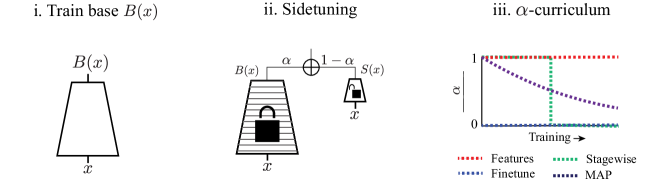
Figure 2: Mechanics of side-tuning. (i) Side-tuning takes some core network and adapts it to a new task by training a side network. (ii) Connectivity structure when using side-tuning along with $\alpha$-blending. (iii) Some of the existing common adaptation methods turn out to be special cases of an alpha blending with a side network. In particular: fine-tuning, feature extraction, and other approaches are side-tuning with a fixed curriculum on the blending parameter $\alpha$, as shown in the plot.

3.1 Architectural Elements

Base Model. The base model $B(x)$ provides some core cognition or perception, and we put no restrictions on how $B(x)$ is computed. We never update $B(x)$, and in our approach it has zero learnable parameters. $B(x)$ could be a decision tree or an oracle for another task (experiments with this setup shown in Section 4.4). We consider several choices for $B(x)$ in Section 4.4, but the simplest choice is just a pretrained network.

Side Model. Unlike the base model, the side network, $S(x)$, is updated during training; learning a residual that we apply on top the base representation. One crucial component of the framework is that the complexity of the side network can scale to the difficulty of the problem at hand. When the base is relevant and requires only a minor update, a very simple side network can suffice.

Since the side network’s role is to amend the base network to a new task, we initialize the side network as a copy of the base. When the forms of the base and side networks differ, we initialize the side network through knowledge distillation [9]. We investigate side network design decisions in Sec. 4.4. In general, we found side-tuning to perform well in a variety of settings and setups.

Combining Base and Side Representations.

Side-tuning admits many options for the combination operator, $\oplus$, and we compare several in Section 4.5. We observe that alpha blending, $B(x)\oplus S(x)~{}\raisebox{-0.15pt}{$\triangleq$}~{}\alpha B(x)+(1-\alpha)S(x)$, where $\alpha$ is treated as a learnable parameter works well and $\alpha$ correlates with task relevance (see Section 4.4).

While simple, alpha blending is expressive enough that it encompasses several common transfer learning approaches. As shown in Figure 2(iii), side-tuning is equivalent to feature extraction when $\alpha=1$. When $\alpha=0$, side-tuning is instead equivalent to fine-tuning if the side network has the same architecture the base. If we allow $\alpha$ to vary during training, then switching $\alpha$ from 1 to 0 is equivalent to the common (stage-wise) training curriculum in RL where a policy is trained on top of some fixed features that are unlocked partway through training.

When minimizing estimation error there is often a tradeoff between the bias and variance contributions [7] (see Table 1). Feature extraction locks the weights and corresponds to a point-mass prior while fine-tuning is an uninformative prior yielding a low-bias high-variance estimator. Side-tuning aims to leverage the (useful) bias from those original features while making the representation asymptotically consistent through updates to the residual side-network .

Given the bias-variance interpretation, a notable curriculum for $\alpha$ during training is $\alpha(N)=\frac{k}{k+N}$ for $k>0$ (hyperbolic decay) where N is the number of training epochs. This curriculum, placing less weight on the prior as more evidence accumulates, is suggestive of a maximum a posteriori estimate and, like the MAP estimate, it converges to the MLE (fine-tuning).

3.2 Side-Tuning for Incremental Learning

We often care about the performance not only on the current target task but also on the previously learned tasks. This is the case for incremental learning, where we want an agent that can learn a sequence of tasks $\mathcal{T}_{1},...,\mathcal{T}_{m}$ and is capable of reasonable performance across the entire set at the end of training. In this paradigm, catastrophic forgetting (diminished performance on $\{\mathcal{T}_{1},...,\mathcal{T}_{m-1}\}$ due to learning $\mathcal{T}_{m}$) becomes a major issue.

In our experiments, we dedicate one new side network to each task. We define a task $\mathcal{T}:x\mapsto P(Y)$ as a mapping from inputs, $x$, to a probability distribution over the output space, $Y$. For example, $x$ is an RGB image mapped to probabilities over object classes, $Y$. Datasets for a task are a set of pairs $\{(x,y)~{}|~{}y\sim\mathcal{T}(x)\}$. For task $\mathcal{T}_{t}$, our loss function is

$$L(x_{t},y_{t})=\lVert D_{t}(\alpha_{t}B(x_{t})+(1-\alpha_{t})S_{t}(x_{t}))-y_{t}\rVert$$

where $t$ is the task number and $D_{t}$ is some decoder readout of the side-tuning representation. This simple approach leads to the training curve in Figure 3 with no possible catastrophic forgetting. Furthermore, since side-tuning is independent of task order, training does not slow down as training progresses. We observe that this approach provides a strong baseline for incremental learning, outperforming existing approaches in the literature while using fewer parameters on more tasks (in Section 4.2).

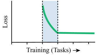
Figure 3: Theoretical learning curve of side-tuning. The model learns during task-specific training and those weights are subsequently frozen, preserving performance.

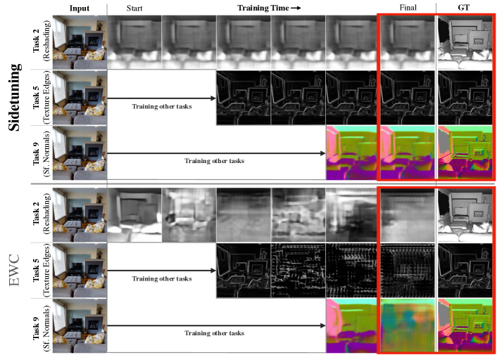
Figure 4: Side-tuning does not forget in incremental learning. Qualitative results for iTaskonomy with additive learning (side-tuning, top 3 rows) and constraint-based substitutive learning (EWC, bottom 3 rows). Each row contains results for one task and columns show how predictions change over the course of training. Predictions from EWC quickly degrade over time, showing that EWC catastrophically forgets. Predictions from side-tuning do not degrade, and the initial quality is better in later tasks (e.g. compare the table in surface normals). We provide additional comparisons (including for PSP, PNN) in the supplementary.

Side-tuning naturally handles other continuous learning scenarios besides incremental learning. A related problem is that of continuous adaptation, where the agent needs to perform well (e.g. minimizing regret) on a stream of tasks with undefined boundaries and where there might very little data per task and no task repeats. As we show in Section 4.2, inflexibility becomes a serious problem for constraint-based methods and task-specific performance declines after learning more than a handful of tasks. Moreover, continuous adaptation requires an online method as task boundaries must be detected and data cannot be replayed (e.g. to generate constraints for EWC).

Side-tuning could be applied to continuous adaptation by keeping a small working memory of cheap side networks that constantly adapt the base network to the input task. These side networks are small, easy to train, and when one of the networks begins performing poorly (e.g. signaling a distribution shift) that network can simply be discarded. This is an online approach, and online adaptation with small cheap networks has found recent success (e.g. in [20]).

4 Experiments

In the first section we show that when applied to the incremental learning setup, side-tuning compares favorably to existing approaches on both iCIFAR and the more challenging iTaskonomy dataset. We then extend this to multiple domains (computer vision, RL, imitation learning, NLP) in the simplified scenario for $m=2$ tasks (transfer learning). Finally, we interpret side-tuning in a series of analysis experiments.

4.1 Baselines

We provide comparisons of side-tuning against the following methods:

Scratch: The network is initialized with appropriate random weights and trained using minibatch SGD with Adam [11].

Feature extraction (features): The pretrained base network is used as-is and is not updated during training.

Fine-tuning: An umbrella term that encompasses a variety of techniques, we consider a more narrow definition where pretrained weights are used as initialization and then training proceeds as in scratch.

Elastic Weight Consolidation (EWC). A constraint-based substitutive approach from [12]. We use the formulation from [30] which scales better.

Parameter Superposition (PSP): A parameter-masking substitutive approach from [4] that attempts to make tasks independent from one another by mapping the weights to approximately orthogonal spaces.

Progressive Neural Network (PNN): An additive approach from [29] which utilizes many lateral connections between the base and side networks. Requires the architecture of the base and side networks to be the same or similar.

Piggyback (PB): Learns task-dependent binary weight masks [17].

Residual Adapters (RA): An additive approach which learns task-dependent batch-norm and linear layers between layers in an existing network [24, 25].

Independent: Each task uses a pretrained network trained independently for that task. This method uses far more learnable parameters than all the alternatives (e.g. saving a separate ResNet-50 for each task) and achieves strong performance.

4.2 Incremental Learning

On both the incremental Taskonomy [34] (iTaskonomy) and incremental CIFAR (iCIFAR [26]) datasets, side-tuning performs competitively against existing incremental learning approaches while using fewer parameters. On the more challenging Taskonomy dataset, it outperforms other approaches.

• iCIFAR. Comprises 10 subsequent tasks by partitioning CIFAR-100 [26] into 10 disjoint sets of 10-classes each. Images are $32{\times}32$ RGB. First, we pretrain the base network (ResNet-44) on CIFAR-10. We then train on each subtask for 20k steps before moving to the next one. The SotA substitutive baselines (EWC and PSP) update the base network for each task (683K parameters), while side-tuning updates a four layer convolutional network per task (259K parameters after 10 tasks).

• iTaskonomy. Taskonomy [34] is significantly more challenging than CIFAR-100 and includes multiple computer vision tasks beyond object classification: including 2D (e.g. edge detection), 3D (e.g. surface normal estimation), and semantic (e.g. object classification) tasks. We note that approaches which work well on iCIFAR often do quite poorly in the more realistic setting. We created iTaskonomy by selecting all (12) tasks that make predictions from a single RGB image, and then created an incremental learning setup by selecting a random order in which to learn these tasks (starting with curvature). The images are $256{\times}256$ and we use a ResNet-50 for the base network and a 5-layer convolutional network for the side-tuning side network. The number of learnable network parameters used across all tasks is 24.6M for EWC and PSP, and 11.0M for side-tuning.

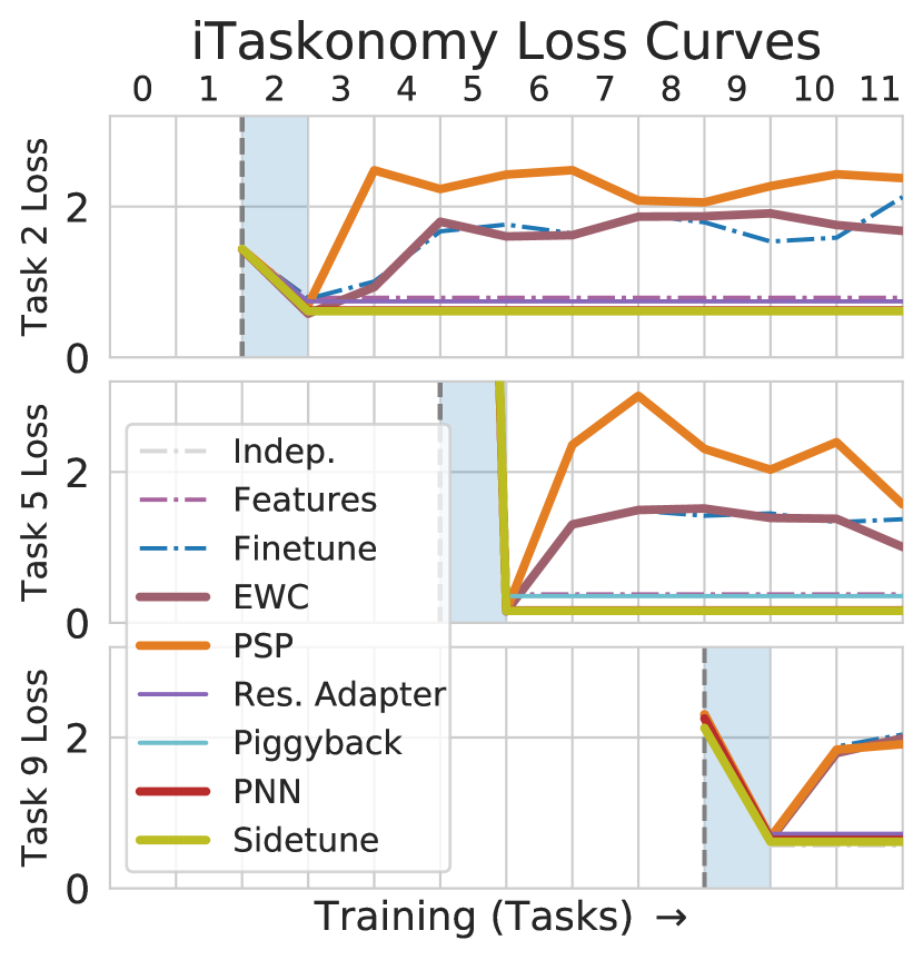
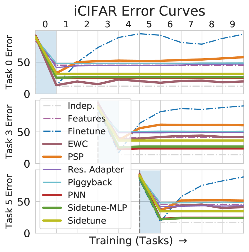
Figure 5: Incremental Learning on iTaskonomy and iCIFAR. The above curves show loss and error for three tasks on iTaskonomy (left) and iCIFAR (right) datasets. The fact that side-tuning losses are flat after training (as we go right) shows that it does not forget previously learned tasks. That performance remains consistent even on later tasks (as we go down), showing that side-tuning does not become rigid. Substitutive methods show clear forgetting (e.g. PSP) and/or rigidity (e.g. EWC). In iTaskonomy, PNN and Independent are hidden under Sidetune.

4.2.1 Catastrophic Forgetting

As expected, there is no catastrophic forgetting in side-tuning and other additive methods. Figure 5 shows that the error for side-tuning does not increase after training (blue shaded region), while it increases sharply for the substitutive methods on both iTaskonomy and iCIFAR.

The difference is meaningful, and Figure 4 shows sample predictions from side-tuning and EWC for a few tasks during and after training. As is evident from the bottom rows, EWC exhibits catastrophic forgetting on all tasks (worse image quality as we move right). In contrast, side-tuning (top) shows no forgetting and the final predictions are significantly closer to the ground-truth (boxed red).

4.2.2 Rigidity

Side-tuning learns later tasks as easily as the first, while constraint-based methods such as EWC stagnate. The predictions for later tasks are significantly better using side-tuning even immediately after training and before any forgetting can occur (e.g., surface normals in Fig. 4).

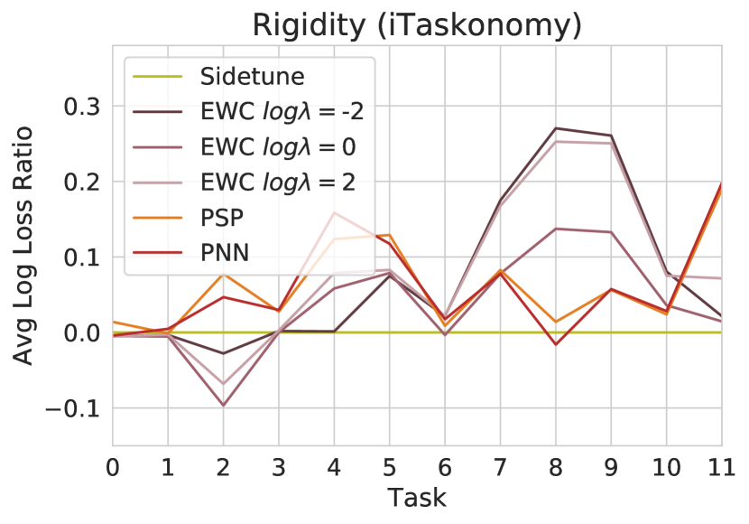
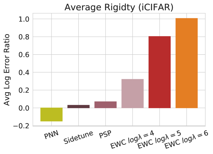
Figure 6: Rigidity (Intransigence) on iTaskonomy and iCIFAR. Side-tuning always learns new tasks easily; EWC becomes increasingly unable to learn new tasks as training progresses. The same trend holds on iCIFAR (right).

Figure 6 quantifies this slowdown. We measure rigidity as the log-ratio of the actual loss of the $i$th task over the loss when that task is instead trained first in the sequence. As expected, side-tuning experiences effectively zero slowdown on both datasets. For EWC, the added constraints make learning new tasks increasingly difficult and rigidity increases with the number of tasks (Fig. 6, left). PNN shows some positive transfer in iCIFAR (negative ratio value), but becomes rigid on the more challenging iTaskonomy, where tasks are more diverse.

4.2.3 Final Performance

Overall, side-tuning significantly outperforms the substitutive methods while using fewer than half the number of trainable parameters. It is comparable with additive methods while remaining remarkably simpler. On iCIFAR, vanilla side-tuning achieves a strong average rank (2.20 of 6, see Table 2) and, when using the same combining operator (MLP) as PNN, is as good as the best-performing model without the additional lateral connections (see Figure 5 right). On iTaskonomy, vanilla side-tuning achieves the best average rank (1.33 of 6, while the next best is 2.42 by PNN, see Table 2).

	Avg. Rank ($\downarrow$)
Method	iTaskonomy	iCIFAR
EWC ($\lambda=10^{0},10^{5}$)	5.25	2.70
PSP	5.25	5.60
Res. Adapter	3.58	4.40
Piggyback	3.17	5.00
PNN	2.42	1.10
Side-tune	1.33	2.20

Table 2: Average rank on iTaskonomy and iCIFAR. Despite being simpler than alternatives, side-tuning generally achieved a better average rank than other approaches. The difference increases on the more challenging Tasknomy dataset, where side-tuning significantly outperformed all tested alternatives.

This is a direct result of the fact (shown above) that side-tuning does not suffer from catastrophic forgetting or rigidity (intransigence). It is not due to the fact that the sidetuning structure is specially designed for these types of image tasks; it is not (we show in Sec. 4.3 that it performs well on other domains). In fact, the much larger networks used in EWC and PSP should achieve better performance on any single task. For example, EWC produces sharper images early on in training, before it has had a chance to accumulate too many constraints (e.g. reshading in Figure 4). But this factor was outweighed by side-tuning’s immunity from the effects of catastrophic forgetting and compunding rigidity.

4.3 Universality of the Experimental Trends

In order to address the possibility that side-tuning is somehow domain- or task-specific, we provide results showing that it is well-behaved in other settings. As the concern with additive learning is mainly that it is too inflexible to learn new tasks, we compare with fine-tuning (which outperforms other incremental learning tasks when forgetting is not an issue). For extremely limited amounts of data, feature extraction can outperform fine-tuning. We show that side-tuning generally performs as well as features or fine-tuning–whichever is better.

Method

Fine-tune

Features

Scratch

Side-tune

Transfer Learning in Taskonomy From Curvature (100/4M ims.) Normals (MSE $\downarrow$) Obj. Cls. (Acc. $\uparrow$) 0.200 / 0.094 24.6 / 62.8 0.204 / 0.117 24.4 / 45.4 0.323 / 0.095 19.1 / 62.3 0.199 / 0.095 24.8 / 63.3
(a)

QA on SQuAD Match ($\uparrow$) Exact F1 79.0 82.2 49.4 49.5 0.98 4.65 79.6 82.7
(b)

Navigation (IL) Nav. Rew. ($\uparrow$) Curv. Denoise 10.5 9.2 11.2 8.2 9.4 9.4 11.1 9.5
(c)

Navigation (RL) Nav. Rew. ($\uparrow$) Curv. Denoise 10.7 10.0 11.9 8.3 7.5 7.5 11.8 10.4
(d)

Table 3: Side-tuning comparisons in other domains. Sidetuning matched the adaptability of fine-tuning on large datasets, while performing as well or better than the best competing method in each domain: (a) In Taskonomy, for Normal Estimation or Object Classification using a base trained for Curvatures and either 100 or 4M images for transfer. Results using Obj. Cls. base are similar and provided in the supplementary materials. (b) In SQuAD v2 question-answering, using BERT instead of a convolutional architecture. (c) In Habitat, learning to navigate by imitating expert navigation policies, using inputs based on either Curvature or Denoising. Finetuning does not perform as well in this domain. (d) Using RL (PPO) and direct interaction instead of supervised learning for navigation.

Transfer learning in Taskonomy. We trained networks to perform one of three target tasks (object classification, surface normal estimation, and curvature estimation) on the Taskonomy dataset [34] and varied the size of the training set $N\in\{100,4\times 10^{6}\}$. In each scenario, the base network was trained (from scratch) to predict one of the non-target tasks. The side network was a copy of the original base network. We experimented with a version of fine-tuning that updated both the base and side networks; the results were similar to standard fine-tuning . In all scenarios, side-tuning successfully matched the adaptiveness of fine-tuning, and significantly outperformed learning from scratch, as shown in Table 3a. The additional structure of the frozen base did not constrain performance with large amounts of data (4M images), and side-tuning performed as well as (and sometimes slightly better than) fine-tuning.

Question-Answering in SQuAD v2. We also evaluated side-tuning on a question-answering task (SQuAD v2 [23]) using a non-convolutional architecture. We use a pretrained BERT [5] model for our base, and a second for the side network. Unlike in the previous experiments, BERT uses attention and no convolutions. Still, side-tuning adapts to the new task just as well as fine-tuning, outperforming features and scratch (Table 3b).

Imitation Learning for Navigation in Habitat. We trained an agent to navigate to a target coordinate in the Habitat environment. The agent is provided with both RGB input image and also an occupancy map of previous locations. The map does not contain any information about the environment—just previous locations. In this section we use Behavior Cloning to train an agent to imitate experts following the shortest path on 49k trajectories in 72 buildings. The agents are evaluated in 14 held-out validation buildings. Depending on what the base network was trained on, the source task might be useful (Curvature) or harmful (Denoising) for imitating the expert and this determines whether features or learning from scratch performs best. Table 3c shows that regardless of the which approach worked best, side-tuning consistently matched or beat it.

Reinforcement Learning for Navigation in Habitat. Using a different learning algorithm (PPO) and direct interaction instead of expert trajectories, we observe identical trends. We trained agents directly in Habitat (74 buildings). Table 3d shows performance in 14 held-out buildings after 10M frames of training. Side-tuning performs comparably to the $\max$ of competing approaches.

4.4 Learning Mechanics in Side-Tuning

Using non-network base models. Since side-tuning treats the base model is a black box, it can be used even when the base model is not a neural network. On iTaskonomy, we show that side-tuning can effectively use ground truth curvature as a base for incremental learning whereas all the methods we compare against cannot use this information (with the exception of feature extraction). Specifically, we resize the curvature image from $256{\times}256{\times}2$ to $32{\times}32{\times}2$ and reshape it to $16{\times}16{\times}8$, the same size as the output of other base models. Side-tuning with ground truth curvature achieves a better rank (4.3) on iTaskonomy than all 20 other methods (excluding Independent, 4.2)

Benefits for intermediate amounts of data. We showed in the previous

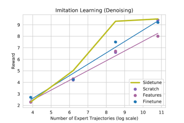
Figure 7: Side-tuning outperformed features and fine-tuning on intermediate amounts of data. Using imitation learning on a point-goal navigation task (setup from [19]).

section that side-tuning performs like the best of $\{\text{features},\text{fine-tuning},\text{scratch}\}$ in domains with abundant or scant data.

In order to test whether side-tuning could profitably synthesize the features with intermediate amounts of data, we evaluated each approach’s ability to learn to navigate using 49, 490, 4900, or 49k expert trajectories and pretrained denoising features. Side-tuning was always the best-performing approach and, on intermediate amounts of data (e.g. 4.9k trajectories), outperformed the other techniques (side-tune 9.3, fine-tune: 7.5, features: 6.7, scratch: 6.6), Figure 7).

Network size. We find that when the base network is large, distilling it into a smaller network and sidetuning will still retain most of the performance. In Figure 8, we explore this in Habitat (RL using $\{\text{curvature},\text{denoise}\}\rightarrow\text{navigation}$), with other results in the supplementary.

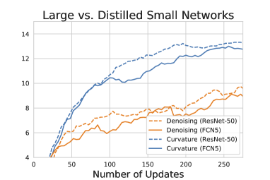
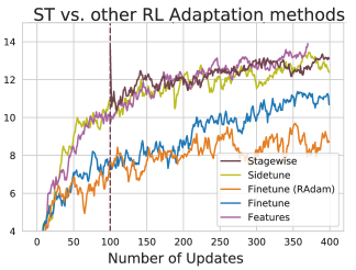
Figure 8: Effect of network size in RL. (Left) The distilled (5-layer) networks perform almost as well as the original ResNet-50 base networks. The choice of which base to use (Curvature vs. Denoising) has a much larger impact. (Right) Fine-tuning, even with RAdam, performed significantly worse than the alternative approaches.

More than just stable updates. In RL, fine-tuning often fails to improve performance. One common rationalization is that the early updates in RL are ‘high variance’. The common stage-wise solution is to first train using fixed features and then unfreeze the weights. We found that this approach performs as well (but no better than) using fixed features–and side-tuning performed as well as both while not being domain-specific (Fig. 8). We tested the ‘high-variance’

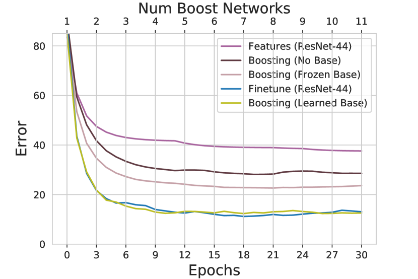
Figure 9: Boosting. Deeper networks outperform many shallow learners.

theory by fine-tuning with both gradient clipping and an optimizer designed to prevent such high-variance updates (RAdam [16]). This provided no benefits over vanilla fine-tuning, suggesting that the benefits of side-tuning are not solely due to gradient stabilization early in training.

Not Boosting. Since the side network learns a residual on top of the base network, could side-tuning be used for boosting? Although network boosting does improve performance on iCIFAR (Figure 9), the parameters would’ve been better used in a deeper network rather than many shallow networks.

4.5 Analysis of Design Choices

We evaluate the effect of our architectural design decisions on task performance.

Base and Side Elements. Side-tuning uses two streams of information - one from the base model and one from the side model. Are both streams necessary? Table 5 shows that on the iTaskonomy experiment performance improves when using both models.

Merge methods. Section 3.1 described different ways to merge the base and side networks. Table 5 evaluates a few of these approaches. Product and alpha-blending are two of the simplest approaches and have little overhead in terms of compute and parameter count. [29] (MLP) and [21] (FiLM) use multi-layer perceptrons to adapt the base network to the new task. Table 5 shows that alpha-blending, MLP, and FiLM are comparable, though the FiLM-based methods achieve marginally better average rank on iTaskonomy. We use alpha-blending as it adds fewer parameters and achieves similar performance.

	Avg. Rank ($\downarrow$)
Method	iTaskonomy
Product (Element-wise)	3.64
Summation ($\alpha$-blending)	2.27
MLP ([29])	2.18
FiLM [21]	1.91

Table 4: Average rank of various merge methods. Alternative feature-wise transformations did not outperform simple $\alpha$-blending in a statistically significant way.

	Avg. Rank ($\downarrow$)
Method	iTaskonomy
Base-Only	2.55
Side-Only	2.10
Side-tuning	1.36

Table 5: Both base and side networks contribute. Performance (average rank on iTaskonomy) improved when using both the base and side model in side-tuning.

Side Network Initialization. A good side network initialization can yield a minor boost in performance. We found that initializing from the base network slightly outperforms a low-energy initialization, which slightly outperforms Xavier initialization. However, we found that these differences were not statistically significant across tasks ($H_{0}:\textit{pretrained}=\textit{xavier};p=0.07$, Wilcoxon signed-rank test). We suspect that initialization might be more important on harder problems. We test this by repeating the analysis without the simple texture-based tasks (2D keypoint + edge detection and autoencoding) and find the difference in initialization is now significant ($p=0.01$).

5 Conclusions and Limitations

We have introduced the side-tuning framework, a simple yet effective approach for additive learning. Since it does not suffer from catastrophic forgetting or rigidity, it is naturally suited to incremental learning. The theoretical advantages are reflected in empirical results, and we found side-tuning to perform on par with or better than many current incremental learning approaches, while being significantly simpler. Experiments demonstrated this in challenging contexts and with various state-of-the-art neural networks across multiple domains.

More complex methods should need to demonstrate clear improvements over simply doing this naïve approach. We see several natural ways to improve it:

Better forward transfer: Our experiments used only a single base and single side network. Leveraging previously trained side networks could yield better performance on later tasks.

Learning when to deploy side networks: Like most incremental learning setups, we assumed that the tasks are presented in a sequence and that task identities are known. Using several active side networks in tandem would provide a natural way to identify task change or distribution shift.

Using side-tuning to measure task relevance: We found that $\alpha$ tracked task relevance in [34], but a more rigorous treatment of the interaction between the base, side, $\alpha$ and final performance could yield insight into how tasks relate.

Acknowledgements: This material is based upon work supported by ONR MURI (N00014-14-1-0671), Vannevar Bush Faculty Fellowship, an Amazon AWS Machine Learning Award, NSF (IIS-1763268), a BDD grant and TRI. Toyota Research Institute (“TRI”) provided funds to assist the authors with research but this article solely reflects the opinions and conclusions of its authors and not TRI or any other Toyota entity.

References

- [1] Bilen, H., Vedaldi, A.: Universal representations: The missing link between faces, text, planktons, and cat breeds. arXiv preprint arXiv:1701.07275 (2017)
- [2] Chaudhry, A., Dokania, P.K., Ajanthan, T., Torr, P.H.: Riemannian walk for incremental learning: Understanding forgetting and intransigence. In: Proceedings of the European Conference on Computer Vision (ECCV). pp. 532–547 (2018)
- [3] Chaudhry, A., Ranzato, M., Rohrbach, M., Elhoseiny, M.: Efficient lifelong learning with a-GEM. In: International Conference on Learning Representations (2019), https://openreview.net/forum?id=Hkf2_sC5FX
- [4] Cheung, B., Terekhov, A., Chen, Y., Agrawal, P., Olshausen, B.: Superposition of many models into one. In: Advances in Neural Information Processing Systems. pp. 10868–10877 (2019)
- [5] Devlin, J., Chang, M., Lee, K., Toutanova, K.: BERT: pre-training of deep bidirectional transformers for language understanding. In: Conference of the North American Chapter of the Association for Computational Linguistics (NAACL) (2019)
- [6] Finn, C., Abbeel, P., Levine, S.: Model-agnostic meta-learning for fast adaptation of deep networks. In: Proceedings of the International Conference on Machine Learning (ICML) (2017)
- [7] Geman, S., Bienenstock, E., Doursat, R.: Neural networks and the bias/variance dilemma. Neural computation 4(1), 1–58 (1992)
- [8] He, K., Zhang, X., Ren, S., Sun, J.: Deep residual learning for image recognition. In: Proceedings of the IEEE conference on computer vision and pattern recognition. pp. 770–778 (2016)
- [9] Hinton, G., Vinyals, O., Dean, J.: Distilling the knowledge in a neural network. arXiv preprint arXiv:1503.02531 (2015)
- [10] Johannink, T., Bahl, S., Nair, A., Luo, J., Kumar, A., Loskyll, M., Ojea, J.A., Solowjow, E., Levine, S.: Residual reinforcement learning for robot control. In: 2019 International Conference on Robotics and Automation (ICRA). pp. 6023–6029. IEEE (2019)
- [11] Kingma, D.P., Ba, J.: Adam: A method for stochastic optimization. International Conference on Learning Representations (2015)
- [12] Kirkpatrick, J., Pascanu, R., Rabinowitz, N., Veness, J., Desjardins, G., Rusu, A.A., Milan, K., Quan, J., Ramalho, T., Grabska-Barwinska, A., et al.: Overcoming catastrophic forgetting in neural networks. Proceedings of the national academy of sciences 114(13), 3521–3526 (2017)
- [13] Leach, P.J.: A critical study of the literature concerning rigidity. British Journal of Social and Clinical Psychology 6(1), 11–22 (1967)
- [14] Lee, J., Joo, D., Hong, H.G., Kim, J.: Residual continual learning. In: AAAI (2020)
- [15] Li, Z., Hoiem, D.: Learning without forgetting. IEEE transactions on pattern analysis and machine intelligence 40(12), 2935–2947 (2017)
- [16] Liu, L., Jiang, H., He, P., Chen, W., Liu, X., Gao, J., Han, J.: On the variance of the adaptive learning rate and beyond. In: Proceedings of the Eighth International Conference on Learning Representations (ICLR 2020) (April 2020)
- [17] Mallya, A., Davis, D., Lazebnik, S.: Piggyback: Adapting a single network to multiple tasks by learning to mask weights. In: Proceedings of the European Conference on Computer Vision (ECCV). pp. 67–82 (2018)
- [18] Mallya, A., Lazebnik, S.: Packnet: Adding multiple tasks to a single network by iterative pruning. In: Proceedings of the IEEE Conference on Computer Vision and Pattern Recognition. pp. 7765–7773 (2018)
- [19] Manolis Savva*, Abhishek Kadian*, Oleksandr Maksymets*, Zhao, Y., Wijmans, E., Jain, B., Straub, J., Liu, J., Koltun, V., Malik, J., Parikh, D., Batra, D.: Habitat: A Platform for Embodied AI Research. In: Proceedings of the IEEE/CVF International Conference on Computer Vision (ICCV) (2019)
- [20] Mullapudi, R.T., Chen, S., Zhang, K., Ramanan, D., Fatahalian, K.: Online model distillation for efficient video inference. In: Proceedings of the IEEE International Conference on Computer Vision. pp. 3573–3582 (2019)
- [21] Perez, E., Strub, F., De Vries, H., Dumoulin, V., Courville, A.: Film: Visual reasoning with a general conditioning layer. In: Thirty-Second AAAI Conference on Artificial Intelligence (2018)
- [22] Raghu, A., Raghu, M., Bengio, S., Vinyals, O.: Rapid Learning or Feature Reuse? Towards Understanding the Effectiveness of MAML. In: International Conference on Learning Representations (ICLR) (2020)
- [23] Rajpurkar, P., Jia, R., Liang, P.: Know what you don’t know: Unanswerable questions for squad. In: Proceedings of the 56th Annual Meeting of the Association for Computational Linguistics (ACL) (2018)
- [24] Rebuffi, S.A., Bilen, H., Vedaldi, A.: Learning multiple visual domains with residual adapters. In: Advances in Neural Information Processing Systems. pp. 506–516 (2017)
- [25] Rebuffi, S.A., Bilen, H., Vedaldi, A.: Efficient parametrization of multi-domain deep neural networks. In: Proceedings of the IEEE Conference on Computer Vision and Pattern Recognition. pp. 8119–8127 (2018)
- [26] Rebuffi, S., Kolesnikov, A., Lampert, C.H.: icarl: Incremental classifier and representation learning. In: IEEE Conference on Computer Vision and Pattern Recognition (CVPR). IEEE (2017)
- [27] Rigidity (psychology): Rigidity (psychology)a — Wikipedia, the free encyclopedia (2020), https://en.wikipedia.org/wiki/Rigidity_(psychology), [Online; accessed 12-July-2020]
- [28] Rosenfeld, A., Tsotsos, J.K.: Incremental learning through deep adaptation. IEEE transactions on pattern analysis and machine intelligence (2018)
- [29] Rusu, A.A., Rabinowitz, N.C., Desjardins, G., Soyer, H., Kirkpatrick, J., Kavukcuoglu, K., Pascanu, R., Hadsell, R.: Progressive neural networks. CoRR abs/1606.04671 (2016), http://arxiv.org/abs/1606.04671
- [30] Schwarz, J., Luketina, J., Czarnecki, W.M., Grabska-Barwinska, A., Teh, Y.W., Pascanu, R., Hadsell, R.: Progress & compress: A scalable framework for continual learning. In: Proceedings of the International Conference on Machine Learning (ICML) (2018)
- [31] Serra, J., Suris, D., Miron, M., Karatzoglou, A.: Overcoming catastrophic forgetting with hard attention to the task. In: International Conference on Machine Learning (2018)
- [32] Sharif Razavian, A., Azizpour, H., Sullivan, J., Carlsson, S.: Cnn features off-the-shelf: an astounding baseline for recognition. In: Proceedings of the IEEE conference on computer vision and pattern recognition workshops. pp. 806–813 (2014)
- [33] Silver, T., Allen, K.R., Tenenbaum, J., Kaelbling, L.P.: Residual policy learning. CoRR abs/1812.06298 (2018), http://arxiv.org/abs/1812.06298
- [34] Zamir, A.R., Sax, A., Shen, W.B., Guibas, L.J., Malik, J., Savarese, S.: Taskonomy: Disentangling task transfer learning. In: IEEE Conference on Computer Vision and Pattern Recognition (CVPR). IEEE (2018)