For a zero-temperature Landau symmetry breaking transition in $n$-dimensional space that completely breaks a finite symmetry $G$, the critical point at the transition has the symmetry $G$. In this paper, we show that the critical point also has a dual symmetry – a $(n-1)$-symmetry described by a higher group when $G$ is Abelian or an algebraic $(n-1)$-symmetry beyond higher group when $G$ is non-Abelian. In fact, any $G$-symmetric system, when restricted to symmetric sub-Hilbert space, can be viewed as a boundary of $G$-gauge theory in one higher dimension. The conservation of gauge charge and gauge flux in the bulk $G$-gauge theory gives rise to the symmetry and the dual symmetry respectively. So any $G$-symmetric system actually has a larger symmetry called categorical symmetry, which is a combination of the symmetry and the dual symmetry. However, part (and only part) of the categorical symmetry must be spontaneously broken in any gapped phase of the system, but there exists a gapless state where the categorical symmetry is not spontaneously broken. Such a gapless state corresponds to the usual critical point of Landau symmetry breaking transition. The above results remain valid even if we expand the notion of symmetry to include higher symmetries and algebraic higher symmetries. Thus our result also applies to critical points for transitions between topological phases of matter. In particular, we show that there can be several critical points for the transition from the 3+1D $Z_{2}$ gauge theory to a trivial phase. The critical point from Higgs condensation has a categorical symmetry formed by a $Z_{2}$ 0-symmetry and its dual – a $Z_{2}$ 2-symmetry, while the critical point of the confinement transition has a categorical symmetry formed by a $Z_{2}$ 1-symmetry and its dual – another $Z_{2}$ 1-symmetry.

Categorical symmetry and non-invertible anomaly
in symmetry-breaking and topological phase transitions

I Introduction

Consider a Landau symmetry breaking transition Landau (1937a, b) in a quantum system in $n$-dimensional space at zero temperature that completely breaks a finite on-site symmetry $G$. The critical point at the transition is a gapless state with $G$-symmetry. When $n=1$, it is well known that the 1+1D gapless critical point has two decoupled sectors at low energies: right-movers and left-movers Ginsparg (1991); Di Francesco et al. (1997). Thus the critical point has a low energy emergent symmetry $G\times G$. In this paper, we would like to show that a similar symmetry “doubling” phenomenon also appears for critical points of Landau symmetry breaking phase transitions in all other dimensions. In this paper we will use $n$d to refer to space dimensions and $(n+1)$D to refer to spacetime dimensions.

In general, the quantum critical point always connects two $n$d phases: a symmetric phase with no ground state degeneracy and a symmetry breaking phase with $|G|$ degenerate ground states. The symmetric phase is characterized by its point-like excitations that carry irreducible representations of $G$. The collection of those point-like excitations, plus their trivial braiding and non-trivial fusion properties, give us a local fusion $n$-category denoted by $n{{\cal R}\text{ep}}(G)$ (see, for example, LABEL:LW170404221,LW180108530,KZ200308898,KZ200514178 and Appendix A). The conservation of those point-like excitations is encoded by the non-trivial fusion of the irreducible representations $R_{q}$’s

$$R_{q_{1}}\otimes R_{q_{2}}=\bigoplus_{q_{3}}N_{q_{1}q_{2}}^{q_{3}}R_{q_{3}},$$ (1)

which reflects the $G$-symmetry. In fact, due to Tannaka duality, the local fusion $n$-category $n{{\cal R}\text{ep}}(G)$ completely characterizes the symmetry group $G$. Since the critical point touches the symmetric phase, the ground state at the critical point is also symmetric under $G$.

The symmetry breaking phase has ground states labeled by the group elements $g\in G$, $|\Psi_{g}\rangle$, that is not invariant under the symmetry transformation: $U_{h}|\Psi_{g}\rangle=|\Psi_{hg}\rangle,\ g,h\in G$. We can always consider a symmetrized ground state $|\Psi_{0}\rangle=\sum_{g}|\Psi_{g}\rangle$ that is invariant under the symmetry transformation: $U_{h}|\Psi_{0}\rangle=|\Psi_{0}\rangle$. The symmetry breaking phase has domain wall excitations and we only consider the symmetrized states with domain walls. The domain walls can also fuse in a non-trivial way, which form a local fusion $n$-category, denoted by $n{{\cal V}\text{ec}}_{G}$ (see LABEL:KZ200308898,KZ200514178 and Appendix A). The non-trivial fusion also leads to a “conservation” of domain-wall excitations.

It turns out that the “conservation” of $(n-1)$-dimensional domain-wall excitations can be viewed as a result of algebraic higher symmetryKong et al. (2020a, b) generated by closed string operators $W_{q}(S^{1})$ that commute with the lattice Hamiltonian

$$W_{q}(S^{1})H=HW_{q}(S^{1}),$$ (2)

for all the closed loops $S^{1}$ (see Section V). LABEL:KZ200514178 conjectured that there is a generalization of Tannaka duality: a local fusion $n$-category ${\cal R}$ (such as $n{{\cal V}\text{ec}}_{G}$) completely characterizes an algebraic higher symmetry (in the present case, an algebraic $(n-1)$-symmetry). When the symmetry group is Abelian, such an algebraic $(n-1)$-symmetry is a $(n-1)$-symmetry described by a higher group. This special case was discussed in LABEL:GW14125148. When the symmetry group is non-Abelian, such an algebraic $(n-1)$-symmetry is beyond higher group description and is not a $(n-1)$-symmetry.

To contrast higher symmetry (described by higher group) and algebraic higher symmetry (beyond higher group), we note that for group-like higher symmetry, the string operators satisfy a group-like algebra

$$W_{q_{1}}(S^{1})W_{q_{2}}(S^{1})=W_{q_{1}\cdot q_{2}}(S^{1}),$$ (3)

while for algebraic higher symmetry, the string operators satisfy a more general algebra

$$W_{q_{1}}(S^{1})W_{q_{2}}(S^{1})=\sum_{q_{3}}N_{q_{1}q_{2}}^{q_{3}}W_{q_{3}}(S^{1}).$$ (4)

The notion of algebraic higher symmetry has appeared in LABEL:FSh0607247,DR10044725,CY180204445,TW191202817,KZ191213168 for 1+1D conformal field theory (CFT) via non-invertible defect lines and for lattice models in general dimensions in LABEL:KZ200308898,KZ200514178. This generalizes the notion of higher form symmetry Kapustin and Thorngren (2013); Gaiotto et al. (2015); Thorngren and von Keyserlingk (2015); Ibieta-Jimenez et al. (2020); Kobayashi et al. (2019); Lake (2018); Wen (2019); Wan and Wang (2019, 2019) (or higher symmetry Kitaev (2003); Wen (2003); Levin and Wen (2003); Nussinov and Ortiz (2009a, b); Yoshida (2011); Bombín (2014)). A higher symmetry is described by a higher group, while an algebraic higher symmetry is beyond higher groups. The charged excitations (the charge objects) of an algebraic higher symmetry is in general characterized by a local fusion higher category (see LABEL:KZ200514178 and Appendix A).

We see that the $G$-symmetry breaking phase, with domain wall excitations forming $n{{\cal V}\text{ec}}_{G}$, actually has an algebraic $(n-1)$-symmetry, denoted as $G^{(n-1)}$. Since the critical point touches the symmetry breaking phase, the critical point also has the algebraic $(n-1)$-symmetry $G^{(n-1)}$. Therefore, the gapless state, at the critical point of $G$-symmetry breaking transition, has both the $G$ 0-symmetry and the algebraic $(n-1)$-symmetry $G^{(n-1)}$. We call this combined symmetry a categorical symmetry. In fact, the categorical symmetry even appears off the critical point, but in a spontaneously broken form.

There is a holographic way to see the appearance of categorical symmetry in any $G$-symmetric system. We note that when restricted to the symmetric sub-Hilbert space, a $n$d $G$-symmetric system can be viewed as a system that has a non-invertible gravitational anomaly, i.e. can be viewed as the boundary of the $G$-gauge theory in one higher dimensionKong and Wen (2014); Ji and Wen (2019). The bulk gauge charges, when brought to the boundary, are the excitations of the $G$ $0$-symmetry, and the gauge fluxes, brought to the boundary, are excitations of the algebraic $(n-1)$-symmetry. The conservation of the gauge charges and gauge fluxes in $G$-gauge theory in the bulk leads to the $G$ $0$-symmetry and algebraic $(n-1)$-symmetry $G^{(n-1)}$ respectively, in our $G$-symmetric system that corresponds to the boundary (for details, see Section II.4). Therefore, the $G$-symmetric system actually has a larger symmetry – the categorical symmetry, which is a combination of the symmetry (from the conservation of gauge charges) and the algebraic $(n-1)$-symmetry (from the conservation of gauge flux), with non-trivial mutual statistics between gauge charges and gauge flux. Such a categorical symmetry is fully characterized by the $G$-gauge theory in one higher dimension.

Since the gapped boundaries of $G$-gauge theory always come from the condensation of the gauge charges and/or the gauge flux, the gapped ground state of $G$-symmetric system always breaks the categorical symmetry partially, either the $G$-symmetry, or the algebraic $(n-1)$-symmetry, or some other mixtures of the two symmetries. A state with the full categorical symmetry (i.e. both the $G$-symmetry and the algebraic $(n-1)$-symmetry) must be gapless. We show that such a gapless state describes the critical point of the Landau symmetry breaking transition.

More generally, all possible gapless states in a $G$-symmetric system are classified by gapless boundaries of $G$-gauge theory in one higher dimension. This universal emergence of categorical symmetry at critical point, and its origin from non-invertible gravitational anomaly (i.e. topological order in one higher dimension), may help us to systematically understand gapless states of matter.

It is worthwhile to point out that a structure similar to categorical symmetry was found previously in Anti-de Sitter/Conformal field theory (AdS/CFT) correspondenceMaldacena (1998); Witten (1998); Klebanov and Witten (1999); Harlow and Ooguri (2018), where a global symmetry $G$ in a conformal field theory (CFT) at the boundary is related to an appearance of a gauge theory of group $G$ in the bulk. In this paper, we stress that the categorical symmetry encoded by the bulk is actually a bigger symmetry than the usual symmetry at the boundary. We point out that the $G$-symmetric gapless critical theory at the $(n+1)$D boundary actually have both the 0-symmetry $G$ and the dual algebraic $(n-1)$-symmetry, which together form the categorical symmetry. For a more detailed discussion, see Section VIII.

In the following, we begin with studying a few concrete examples, to show the appearance of categorical symmetries in Landau symmetry breaking transitions and in topological phase transitions, as well as neighboring gapped states that partially break the categorical symmetries spontaneously. In Section II, III and IV, we discuss the example of models associated with the $Z_{2}$ group, in $1+1$D, $2+1$D, without and with ’t Hooft anomaly. We introduce the patch operators, as a main tool to detect local charges in sub-Hilbert space that is symmetric under global symmetries. We show how to use the patch operators to describe categorical symmetry. In Section V, we discuss the categorical symmetries in the lattice models with general finite group $G$ in any $n$ spacial dimension. In Section VI, we discuss the emergence of algebraic higher symmetry. In Section VII, we discuss the emergence of categorical symmetry for a set of low energy excitations, and how the categorical symmetry can constrain on the possible phases and phase transitions induced by those low energy excitations. In particular, we discuss how the emergent categorical symmetry determines the duality relations between low energy effective field theories. In Section VIII, we summarize our results and point out its implication for a particular AdS/CFT dual.

II $Z_{2}$ and dual $\widetilde{Z}_{2}$ symmetries in 1+1D Ising model

II.1 Duality transformation in 1+1D Ising model

A common scenario happening at the critical point between the symmetric phase and the symmetry breaking phase is the emergent symmetry. The example we know the best is the Ising transition in one dimension. The paramagnetic phase is $Z_{2}$ symmetric, and the ferromagnetic phase spontaneously breaks the $Z_{2}$ symmetry. The critical point is $Z_{2}$ symmetric. More than that, it also has an additional $Z_{2}$ symmetry Belavin et al. (1984); Zamolodchikov and Fateev (1985); Chang et al. (2019); Verresen et al. (2019); Ji et al. (2020).

To see both $Z_{2}$ symmetries, we consider Ising model on a ring of $L$ sites, where on each site $i$ there are spin-up and spin-down state in the Pauli-$Z_{i}$ basis. So the Hilbert space is ${\cal V}=\otimes_{i=0}^{L-1}\{|\uparrow_{i}\rangle,|\downarrow_{i}\rangle\}$. Each state in the Hilbert space can be also labeled in an alternative way, that is via the absence or presence of a domain wall (DW) in the dual lattice of $L$ links. On each link $i+\frac{1}{2}$, a domain wall means the spins on $i$ and $i+1$ are anti-parallel. It follows that each basis state $|\psi\rangle$ of ${\cal V}$ and its $Z_{2}$ partner $|\psi^{\prime}\rangle$ are labeled by the same kink variable on the dual lattice. So the $Z_{2}$ symmetric state in ${\cal V}$ is labeled uniquely by the DW variable. Moreover, a configuration of odd number of domain walls on links cannot be mapped to any configuration of spins on sites. Thus each DW variable with an even number of DW’s labels a unique $Z_{2}$ symmetric state. Therefore, we say that the $Z_{2}$ symmetric Hilbert space of spins on the sites is in one-to-one correspondence with the Hilbert space of even number of DWs on the links. Each of the Hilbert space is of dimension $2^{L-1}$.

Next, we demonstrate an isomorphism between a set of operators on sites and that on links.

$$X_{i}I_{i+1}\rightarrow\widetilde{X}_{i-\frac{1}{2}}\widetilde{X}_{i+\frac{1}{2}},~{}~{}~{}Z_{i}Z_{i+1}\rightarrow\widetilde{I}_{i-\frac{1}{2}}\widetilde{Z}_{i+\frac{1}{2}}.$$ (5)

Here, we use the following notation,

$$X=\begin{pmatrix}0&1\\ 1&0\end{pmatrix},~{}~{}Z=\begin{pmatrix}1&0\\ 0&-1\end{pmatrix},~{}~{}I=\begin{pmatrix}1&0\\ 0&1\end{pmatrix}.$$ (6)

Physically, the spin-flipping $X_{i}$ is the same as creating two DW’s on $i-\frac{1}{2}$ and $i+\frac{1}{2}$ links, represented by $\widetilde{X}_{i-\frac{1}{2}}\widetilde{X}_{i+\frac{1}{2}}$. The Ising coupling term $Z_{i}Z_{i+1}$ also measures the energy cost of a domain wall, which is represented by $\widetilde{Z}_{i+\frac{1}{2}}$. Formally, the two sets of operators $\{X_{i},Z_{i}Z_{i+1}\}$ and $\{\widetilde{X}_{i-\frac{1}{2}}\widetilde{X}_{i+\frac{1}{2}},\widetilde{Z}_{i+\frac{1}{2}}\}$ are two representations of the same set of operators $\{W_{i},W_{i+\frac{1}{2}}\}$ defined by the operator algebra, for $i=\frac{1}{2},1,\cdots,L$,

(i) $$W_{i}^{2}=1,~{}$$

(ii) $$W_{i}W_{i+\frac{1}{2}}=-W_{i+\frac{1}{2}}W_{i},$$ (7)

(iii) $$[W_{i},W_{j}]=0,~{}|i-j|\geq 1.$$

We also have a further global condition,

$$\begin{split}U_{Z_{2}}=\prod_{i=1,2,\cdots,L}W_{i}=1\,,\\ U_{\widetilde{Z}_{2}}=\prod_{i=\frac{1}{2},\frac{3}{2},\cdots L-\frac{1}{2}}W_{i}=1\,.\end{split}$$ (8)

We have two $2^{L-1}$ dimensional representations of $W_{i}$’s, satisfying these relations (II.1) and (8). In particular, the following Hamiltonian,

$$H=-\sum_{i=1,2\cdots,L}\left(BW_{i}+JW_{i+\frac{1}{2}}\right),$$ (9)

has the same spectrum independent of the representation. In the “spin representation”, the Hamiltonian reduces to

$$\begin{split}&H^{\text{Is}}=-\sum_{i=1,2,\cdots,L}\left(BX_{i}+JZ_{i}Z_{i+1}\right),\\ &U_{Z_{2}}=\prod_{i=1,2,\cdots L}X_{i}=1,~{}~{}U_{\widetilde{Z}_{2}}=Z_{L+1}Z_{1}=1.\end{split}$$ (10)

In the “DW representation”, the Hamiltonian reduces to

$$\begin{split}&H^{\text{DW}}=-\sum_{i=1,2,\cdots,L}\left(B\widetilde{X}_{i-\frac{1}{2}}\widetilde{X}_{i+\frac{1}{2}}+J\widetilde{Z}_{i+\frac{1}{2}}\right),\\ &U_{Z_{2}}=\widetilde{X}_{L+\frac{1}{2}}\widetilde{X}_{\frac{1}{2}}=1,~{}~{}U_{\widetilde{Z}_{2}}=\prod_{i=1,2,\cdots L}\widetilde{Z}_{i-\frac{1}{2}}=1.\end{split}$$ (11)

The unitary transformation (5) between the “spin representation” and “DW representation” is also known as $Z_{2}$ gauging. In the current case, it is also the same as Kramers-Wannier duality.

The Ising model has two exact $Z_{2}$ symmetries. However, in our spin and DW representations, we do not see them simultaneously. In the spin representation, we see one $Z_{2}$ symmetry generated by

$$U_{Z_{2}}=\prod_{i=1,\cdots,L}X_{i},$$ (12)

which is denoted as $Z_{2}$. In the DW representation, we see the other $Z_{2}$ symmetry generated by

$$U_{\widetilde{Z}_{2}}=\prod_{i=0,\cdots,L}\widetilde{Z}_{i+\frac{1}{2}},$$ (13)

which is denoted as $\widetilde{Z}_{2}$. $Z_{2}$ and $\widetilde{Z}_{2}$ are two different $Z_{2}$ symmetries, as one can see from their different charge excitations. Despite we only see one symmetry in one formulation, the Ising model actually have both symmetries. The combination of the two symmetries is the so-called categorical symmetry, which is denoted as $Z_{2}\vee\widetilde{Z}_{2}$. Certainly, the critical model at $|J|=|B|$ also have the $Z_{2}\vee\widetilde{Z}_{2}$ categorical symmetry (see Fig. 1). It is interesting to note that, in the ground state of the Ising model, either $Z_{2}\vee\widetilde{Z}_{2}$ categorical symmetry is spontaneously broken partially (for example, one of the $Z_{2}$ is spontaneously broken) or the ground state is gaplessLevin (2020). This indicates that $Z_{2}$ symmetry and the dual $\widetilde{Z}_{2}$ symmetry are not independent. There must be a special relation between them. To reveal it, we need to discuss the charge excitations of the symmetries.

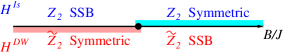
Figure 1: The same Ising model can be describe by $H^{\text{Is}}$ or by $H^{\text{DW}}$. The $Z_{2}$ symmetry is explicit in the $H^{\text{Is}}$ description, while the $\widetilde{Z}_{2}$ dual symmetry is explicit in the $H^{\text{DW}}$ description. The Ising model has both the $Z_{2}$ symmetry and $\widetilde{Z}_{2}$ dual symmetry. The ground state usually spontaneously breaks one of the symmetries, except at the $B=J$ critical point, where both the symmetry and the dual symmetry (i.e. the full $Z_{2}\vee\widetilde{Z}_{2}$ categorical symmetry) are not spontaneously broken.

II.2 Patch symmetry transformation

In the above, we argue that the lattice model eqn. (9) (or eqn. (10) or eqn. (11)) in the symmetric sub-Hilbert space has two $Z_{2}$ symmetries generated by $U_{Z_{2}}$ and $U_{\widetilde{Z}_{2}}$. But in the symmetric sub-Hilbert space, the two operators are identity operator $U_{Z_{2}}=U_{\widetilde{Z}_{2}}=1$. The two $Z_{2}$ transformations are do-nothing transformations. So what does it mean that the lattice model in symmetric sub-Hilbert space has two $Z_{2}$ symmetries? In this section, we are going to solve this problem by introducing patch symmetry transformations. This is a new and better way to view symmetries in local quantum systems. Such kind of operators have been studied mostly for continuous global symmetries, known in the literature Harlow and Ooguri (2019) as splittable symmetry operators, dating back to 1980s Doplicher (1982); Doplicher and Longo (1983); Buchholz et al. (1986). Its one dimensional version also appears in Levin (2020).

We notice that even though $U_{Z_{2}}$ and $U_{\widetilde{Z}_{2}}$ act as identity in the symmetric sub-Hilbert space, the sub-Hilbert space is not consisted of only a vacuum state. Rather, spin flip as well as domain wall excitations are still present, and they are subject to mod-2 conservations. So the effect of two $Z_{2}$ symmetries is still there within the symmetric sub-Hilbert space. For example, there exists a state on the ring containing two well-separated spin excitations, each carrying the $U_{Z_{2}}$-charge $1$ while the total $U_{Z_{2}}$-charge is $0$ mod 2. How to measure the local $U_{Z_{2}}$-charge via a symmetry transformation operator?

To diagnose the conserved local charges of $U_{Z_{2}}$ and $U_{\widetilde{Z}_{2}}$ symmetries, subjective to conservation laws, we now introduce two sets of patch symmetry operators for the simple model eqn. (10) or eqn. (11).

The first patch symmetry is generated by the following transformations,

$$U_{Z_{2}}(i,j)=\prod_{l=i}^{j}X_{l},~{}~{}~{}\text{for~{}~{}}j-i\geq 0,$$ (14)

which are required to act within the symmetric sub-Hilbert space. They also have the properties that for any $j-i\geq 1,j^{\prime}-i^{\prime}\geq 0$,

$$\begin{split}&U_{Z_{2}}(i,k)=U_{Z_{2}}(i,j)U_{Z_{2}}(j+1,k),\\ &U_{Z_{2}}(i,j)^{2}=1,\ \ \ [U_{Z_{2}}(i,j),U_{Z_{2}}(i^{\prime},j^{\prime})]=0.\\ \end{split}$$ (15)

In condensed matter physics, a symmetry is simply a constraint on the lattice Hamiltonian $H$. We usually describe such a constraint as a constraint on the Hamiltonian $H$ as a whole. Under such constraint, the Hamiltonian $H$ is allowed to be local or non-local. This actually is a drawback of the standard formulation of the symmetry, since its does not care about the locality of the Hamiltonian. In our new description of symmetry, using patch operators, we assume the Hamiltonian $H$ to be sum of local operators $H=\sum_{x}O_{x}$. Then the constraint on the Hamiltonian $H$ is expressed in terms of the constraint on the local terms $O_{x}$. In other words, a system is said to have the patch symmetry, if it has the following properties: each local term in the Hamiltonian commutes with all the patch symmetry operators, as long as the local term is far away from the boundary of the patch operator. For example, if $H_{l}$ is a term on ${l,l+1}$, and if it commutes with all patch symmetry operators $U_{Z_{2}}(i,j)$ with $i,j\neq l,l+1$, this term is symmetric under the patch symmetry. If every term in the Hamiltonian has this property, we say the Hamiltonian has the patch symmetry.

Each patch symmetry operator $U_{Z_{2}}(i,j)$ measures the $Z_{2}$ spin excitations in its “bulk”, the sites covered by the patch, from site $i$ to site $j$. More precisely, a local operator $\psi_{k}$ carries $Z_{2}$-charge $1$ if it satisfies

$$U_{Z_{2}}(i,j)\psi_{k}=-\psi_{k}U_{Z_{2}}(i,j),\ \ \ \ i\ll k\ll j.$$ (16)

$\psi_{k}\psi_{l}$ creates two $Z_{2}$-charges at $k$ and $l$ within the symmetric sub-Hilbert space.

In eqn. (14), the patch symmetry operator is given in the spin-representation. In the DW representation, it will has a form

$$U_{Z_{2}}(i,j)=\widetilde{X}_{i-\frac{1}{2}}\widetilde{X}_{j+\frac{1}{2}},$$ (17)

which has a trivial “body of the string” but only two end points. By the definition given above about a system symmetric under the patch symmetry, and due to the trivial bulk, any local Hamiltonian in the DW representation is symmetric under $U_{Z_{2}}(i,j)$. We may also take the patch operators $U_{Z_{2}}(i,j)$ as creating a pair of $\widetilde{Z}_{2}$-charged excitations (i.e. a pair of $Z_{2}$ domain walls) at the ending links $i-\frac{1}{2}$ and $j+\frac{1}{2}$.

The second patch symmetry is generated by the following operators, in the spin- and DW-representations

$$U_{\widetilde{Z}_{2}}(i,j)=Z_{i}Z_{j},\ \ \ \ U_{\widetilde{Z}_{2}}(i,j)=\prod_{l=i}^{j-1}\widetilde{Z}_{l+\frac{1}{2}},$$ (18)

which have the properties that they act within the symmetric sub-Hilbert space, for any $j-i\geq 1,j^{\prime}-i^{\prime}\geq 1$,

$$\begin{split}U_{\widetilde{Z}_{2}}(i,k)&=U_{\widetilde{Z}_{2}}(i,j)U_{\widetilde{Z}_{2}}(j,k),\\ U_{\widetilde{Z}_{2}}(i,j)^{2}&=1,\ \ \ [U_{\widetilde{Z}_{2}}(i,j),U_{\widetilde{Z}_{2}}(i^{\prime},j^{\prime})]=0.\end{split}$$ (19)

We see that any local Hamiltonian in spin-representation has the $U_{\widetilde{Z}_{2}}$ symmetry. However, for the Hamiltonian in the “DW representation”, the second patch symmetry gives rise to a non-trivial constraint on the Hamiltonian. These symmetry operators serve to measure local domain wall excitations. We can see this in the spin representation, i.e. when $Z_{i}$ and $Z_{j}$ have opposite sign, i.e. there is domain between $i$ and $j$, then $U_{\widetilde{Z}_{2}}(i,j)=Z_{i}Z_{j}=-1$.

In summary, we identify two patch symmetries, each is generated by a set of commuting operators. The two kinds of patch symmetries act non-trivially even in the symmetric sub-Hilbert space, and can impose constraints on Hamiltonians. The symmetric Hamiltonians ensure the mod-2 conservation of the $Z_{2}$-charges and domain walls.

The patch symmetry transformations also allow us to identify a special new property – the “mutual statistics” between charges of the two global symmetries (or patch symmetries), given by the following relation, for $i\ll i^{\prime}\ll j\ll j^{\prime}$,

$$U_{Z_{2}}(i,j)U_{\widetilde{Z}_{2}}(i^{\prime},j^{\prime}) =-U_{\widetilde{Z}_{2}}(i^{\prime},j^{\prime})U_{Z_{2}}(i,j).$$ (20)

In other ways, a local charge under the $Z_{2}$ global symmetry is created at each end point of a $\widetilde{Z}_{2}$ patch operator. If a $Z_{2}$ symmetry patch and a $\widetilde{Z}_{2}$ symmetry patch partially overlap, the single charge at one end point can be measured by the $Z_{2}$ patch symmetry operator. All such statements remain true if exchanging $Z_{2}$ and $\widetilde{Z}_{2}$. We call such properties the “mutual statistics” between charges of the two patch symmetries. The collection of all patch symmetries is nothing but the categorical symmetry. The property (20) justifies the symmetry to be $Z_{2}\vee\widetilde{Z}_{2}$, rather than $Z_{2}\times\widetilde{Z}_{2}$.

We see that the categorical symmetry in a system can be fully described by a set of patch operators, without the need to go to one higher dimension. Alternatively, later in section II.4, we describe the categorical symmetry in terms of the topological order and the associated long-range entanglement, by viewing the system as a boundary of a topological order in one higher dimension. The above result confirms that the categorical symmetry is indeed a property of the system itself.

Note that $\langle U_{\widetilde{Z}_{2}}(i,j)\rangle$ also turns out to be the correlation of order parameters of the $Z_{2}$-symmetry, while $\langle U_{Z_{2}}(i,j)\rangle$ happens to be the correlation of order parameters of the $\widetilde{Z}_{2}$-symmetry. If there is a state, where both the $Z_{2}$-symmetry and the $\widetilde{Z}_{2}$-symmetry are spontaneously broken, then $U_{\widetilde{Z}_{2}}(i,j)$ and $U_{Z_{2}}(i,j)$ behave like $c$-numbers for the state. This will contradict with eqn. (20). Therefore, the $Z_{2}$-symmetry and the $\widetilde{Z}_{2}$-symmetry cannot be both spontaneously broken. A more rigorous proof was given in LABEL:L190309028.

II.3 A model where both $Z_{2}$ symmetry and dual $\widetilde{Z}_{2}$ symmetry are explicit

The Ising model in its spin representation eqn. (10) or in its DW representation eqn. (11) only shows one of the $Z_{2}$ and dual $\widetilde{Z}_{2}$ symmetries explicitly. In this section, we will discuss the third representation of the Ising model, where both the $Z_{2}$ and dual $\widetilde{Z}_{2}$ symmetries appear explicitly.

Consider a model with spin-up and down states defined on $N$ sites as well as on $N$ links. So we begin with $2^{2N}$ states. The model has the following Hamiltonian,

$$H= -\sum_{i}\left(B\widetilde{X}_{i-\frac{1}{2}}X_{i}\widetilde{X}_{i+\frac{1}{2}}+J\widetilde{Z}_{i+\frac{1}{2}}\right)$$

$$+U(1-Z_{i}\widetilde{Z}_{i+\frac{1}{2}}Z_{i+1}).$$ (21)

We only consider the low energy limit $U\rightarrow\infty$ limit, as well as under the projection $U_{Z_{2}}=\prod_{i}X_{i}=1$. (Note that the $B$-term and the $J$-term commute with the constraint $U$-term and $U_{Z_{2}}$.) In the restricted low energy sector, we are left with $2^{N-1}$ states. The above Hamiltonian is conventionally known as describing $Z_{2}$ matter field coupled to $Z_{2}$ gauge field in 1+1D dual lattice. The Ising model (10) with the $Z_{2}$ symmetric sub-Hilbert space turns out to be equivalent as the low energy effective theory of the above model with $B,\ J>0$ and $U\rightarrow+\infty$. There are more than one way to proof this. In Appendix B, we give a proof using the stabilizer formalism in quantum information. In the next subsection, we will show the same Hamiltonian together with the same projected sub-Hilbert space arises as the boundary theory of the $Z_{2}$ topological order.

The $Z_{2}\times\widetilde{Z}_{2}$ symmetry (or more precisely, the $Z_{2}\vee\widetilde{Z}_{2}$ categorical symmetry) is explicit in the above model, which is generated by $U_{Z_{2}}$ in eqn. (12) and $U_{\widetilde{Z}_{2}}$ in eqn. (13) as an on-site symmetry of the model. Even though the $Z_{2}\times\widetilde{Z}_{2}$ symmetry is on site in the model (II.3), it is anomalous when restricted in the low energy sector in the sense that in $U=+\infty$ limit, the model cannot have gapped ground state that breaks the full $Z_{2}\times\widetilde{Z}_{2}$ symmetry. (Certainly, when $U<J,B$, the model can have a gapped ground state that breaks the full $Z_{2}\times\widetilde{Z}_{2}$ symmetry, such as when $J=B=1,U=0$.) In $U=+\infty$ limit, only the gapless state at $J=B$ has the full $Z_{2}\times\widetilde{Z}_{2}$ symmetry that is not spontaneously broken.

What are the patch symmetry transformations for the $Z_{2}$ and $\widetilde{Z}_{2}$ symmetry? The first guess are

$$U_{Z_{2}}(i,j)=\prod_{k=i}^{j}X_{k},\ \ \ \ \ U_{\widetilde{Z}_{2}}(i,j)=\prod_{k=i}^{j}\widetilde{Z}_{k+\frac{1}{2}}.$$ (22)

But $U_{Z_{2}}(i,j)=\prod_{k=i}^{j}X_{k}$ does not act within the low energy sub-Hilbert space (in $U=+\infty$ limit). To get around, we modify it at the boundary, which leads to

$$\begin{split}U_{Z_{2}}(i,j)&=\widetilde{X}_{i-\frac{1}{2}}\Big{(}\prod_{k=i}^{j}X_{k}\Big{)}\widetilde{X}_{j+\frac{1}{2}},\\ U_{\widetilde{Z}_{2}}(i,j)&=\Big{(}\prod_{k=i}^{j}\widetilde{Z}_{k+\frac{1}{2}}\Big{)}.\end{split}$$ (23)

The two sets of patch symmetry transformations still satisfy the algebras eqn. (15) and eqn. (19) as previously. Most importantly, the two sets of patch symmetry transformations have a $\pi$ “mutual statistics” described by eqn. (20). It is this property of the patch operators that we mean the symmetry we consider is $Z_{2}\vee\widetilde{Z}_{2}$, but not $Z_{2}\times\widetilde{Z}_{2}$. One can also easily check that the local terms in the Hamiltonian (II.3) commute with the patch symmetry transformations when far away from the boundary. So the Hamiltonian (II.3) has the $Z_{2}$ and $\widetilde{Z}_{2}$ patch symmetries. In short, although the global symmetry transformation of $Z_{2}$ and $\widetilde{Z}_{2}$ commute, yet the patch operators, which create charges at their end points, do not commute in the low energy sub-Hilbert space limit when $U\rightarrow\infty$.

We would like to remark that the same symmetry can be described by different yet equivalent choices of patch symmetry transformations. Two sets of patch symmetry transformations are equivalent if the patch symmetry transformations only differ by “local neutral operators” at the boundary of the patches. Here a “local neutral operator” is a local operator that commutes with all patch symmetry transformations whose boundary is far away from the operator. The “mutual statistics” of the patch symmetry transformations is not affected by those local neutral operators. For example, we may instead choose $U_{Z_{2}}(i,j)=\widetilde{Y}_{i-\frac{1}{2}}\left(\prod_{k=i}^{j}X_{k}\right)\widetilde{Y}_{j+\frac{1}{2}}$ in (23).

II.4 Symmetric sector of 1+1D Ising model as boundary of 2+1D $Z_{2}$ topological order

In the previous section, we discuss the anomaly property of $Z_{2}\vee\widetilde{Z}_{2}$ categorical symmetry, the mutual statistics of $Z_{2}$ and $\widetilde{Z}_{2}$ charges in the low energy limit. This forbids a symmetric gapped ground state within the low energy sector. In this section, we will show that the anomaly property of the $Z_{2}\vee\widetilde{Z}_{2}$ categorical symmetry is actually an effect of non-invertible gravitational anomaly Ji and Wen (2019). More precisely, the theory with the categorical symmetry can be a boundary theory of a $Z_{2}$ topological order in one higher dimension. The charges and their mutual statistics eqn. (20) of the symmetry is determined by the bulk topological order. To see the non-invertible gravitational anomaly in the 1+1D Ising model, we concentrate on the so-called symmetric sub-Hilbert space ${\cal V}_{\text{symm}}$ that is invariant under the $U_{Z_{2}}$ transformation. The space ${\cal V}_{\text{symm}}$ of a $L$-site system does not have tensor product expansion of the form $\otimes_{i=1}^{L}{\cal V}_{i}$

$${\cal V}_{\text{symm}}\neq\otimes_{i=1}^{L}{\cal V}_{i}.$$ (24)

Thus the symmetric sector of the Ising model can be viewed as having a non-invertible gravitational anomaly Ji and Wen (2019). Indeed, the symmetric sector of the Ising model can be viewed as a boundary of 2+1D $Z_{2}$ topological order (the topological order characterized by $Z_{2}$ gauge theory), and thus has a 1+1D non-invertible gravitational anomaly characterized by 2+1D $Z_{2}$ topological order Ji and Wen (2019).

A 2+1D $Z_{2}$ topological order has four types of excitations $\mathbf{1},e,m,f$. Here $\mathbf{1}$ is the trivial excitation, and $e,m,f$ are topological excitation with mutual $\pi$-statistics between any two different ones. $\mathbf{1},e,m$ are bosons and $f$ is a fermion. They satisfy the following fusion relations,

$$e\otimes e=\mathbf{1},\ \ m\otimes m=\mathbf{1},\ \ f\otimes f=\mathbf{1},\ \ e\otimes m=f.$$ (25)

Let us construct the boundary effective theory for the $m$ condensed boundary of $Z_{2}$ topological order. Such a boundary contains a gapped excitation that corresponds to the $e$-type particle. One might expect a second boundary excitation corresponding to the $f$-type particle. However, since $m$ is condensed on the boundary, the $e$-type particle and the $f$-type particle are actual equivalent on the boundary. The simplest boundary effective lattice Hamiltonian that describes the gapped $e$-type particles has a form (on a ring)

$$H=-B\sum_{i}X_{i},\ \ \ \ B>0.$$ (26)

Here a spin $X_{i}=1$ corresponds to an empty site and a spin $X_{i}=-1$ corresponds to a site occupied with an $e$-type particle (with $2B$ as its energy gap). However, the boundary Hilbert space does not have a direct product decomposition $\otimes_{i}{\cal V}_{i}$, due to the constraint

$$\prod_{i}X_{i}=1,$$ (27)

since the number of the $e$-type particles on the boundary must be even (assume the bulk has no topological excitations). This is a reflection of non-invertible gravitational anomaly. A more general boundary effective theory may have a form

$$H^{\text{Is}}_{P}=-B\sum_{i=1}^{L}X_{i}-J\sum_{i=1}^{L}Z_{i}Z_{i+1},$$ (28)

where $Z_{L+1}\equiv Z_{1}$ and $Z_{i}Z_{i+1}$ creates a pair of the $e$-type particles, or move an $e$-type particle from one site to another.

In the above, we have shown that a boundary of 2+1D $Z_{2}$ topological order can be described by eqn. (28). The low energy sector of the model eqn. (II.3) also describes the boundary of the 2+1D $Z_{2}$ gauge theory with $Z_{2}$-charge $e$ and $Z_{2}$-vortex $m$, where $e$ and $m$ particle has low energies on the boundary. An $e$ particle on the boundary corresponds to $X_{i}=-1$ and a $m$ particle corresponds to $\widetilde{Z}_{i+\frac{1}{2}}=-1$ in eqn. (II.3). The $Z_{2}\times\widetilde{Z}_{2}$ symmetry is the mod-2 conservation of $e$ and $m$ particles. This explains the $Z_{2}\times\widetilde{Z}_{2}$ symmetry in the symmetric sector of the Ising model. Note that, on the boundary, we may have a $e$ or $m$ condensation. The condensations may spontaneously break the $Z_{2}\times\widetilde{Z}_{2}$ symmetry in the ground state. However, the model itself (given by the Hamiltonian and the sub-Hilbert space) always has $Z_{2}\times\widetilde{Z}_{2}$ symmetry.

It is more precise to refer the $Z_{2}\times\widetilde{Z}_{2}$ symmetry as $Z_{2}\vee\widetilde{Z}_{2}$ categorical symmetry. This is because the $Z_{2}$ and $\widetilde{Z}_{2}$ symmetries are not independent. The $Z_{2}$-charge (the $e$ particle) and the $\widetilde{Z}_{2}$-charge (the $m$ particle) have a $\pi$ mutual statistics, when viewed as particles in one higher dimension. This gives rise to eqn. (20). The term $Z_{2}\vee\widetilde{Z}_{2}$ categorical symmetry includes such non-trivial “mutual statistics” between the $Z_{2}$ and $\widetilde{Z}_{2}$ symmetry.

The mutual $\pi$-statistics between $e$ and $m$ in the 2+1D bulk is encoded at boundary by requiring the $Z_{2}$ domain wall to carry $\widetilde{Z}_{2}$ charge and the $\widetilde{Z}_{2}$ domain wall to carry $Z_{2}$ charge. This non-trivial mutual statistics has a highly non-trivial effect: in a gapped ground state, one and only one of $Z_{2}$ and $\widetilde{Z}_{2}$ symmetries must be spontaneously broken Levin (2020). Thus, a symmetric state that does not break the $Z_{2}\vee\widetilde{Z}_{2}$ categorical symmetry must be gapless. This is a consequence of 1+1D non-invertible gravitational anomaly Ji and Wen (2019) characterized by 2+1D $Z_{2}$ topological order (i.e. $Z_{2}$ gauge theory).

To summarize, in the above, we considered the boundary of 2+1D $Z_{2}$ topological order. We argued that a boundary (gapped or gapless), as a system (with the symmetric sub-Hilbert space), always has a $Z_{2}\vee\widetilde{Z}_{2}$ categorical symmetry. In contrast, a gapped boundary, as a state, has a partially spontaneous broken categorical symmetry, while one of the gapless boundaries, as a state, has the full categorical symmetry. Next, let us discuss patch symmetry transformations for the boundary of 2+1D $Z_{2}$ topological order, that describe the $Z_{2}\vee\widetilde{Z}_{2}$ categorical symmetry.

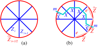
Figure 2: The reduced lattice, where spin-$\frac{1}{2}$ degrees of freedom live on the links.

We start with the bulk Hamiltonian for the $Z_{2}$ topological order on a square lattice, where spin-$\frac{1}{2}$ degrees of freedom live on the links:

$$H^{\text{bulk}}=-U\sum_{s}\prod_{s\subset\partial l}X_{l}-U\sum_{p}\prod_{l\subset\partial p}Z_{l},$$ (29)

where $s$ labels the sites, $l$ the links, and $p$ the plaquettes. $\sum_{s}$ sums over all the sites in the bulk (i.e. off the boundary), and $\sum_{p}$ sums over all the plaquettes. On the boundary, we can have any local Hamiltonian $H^{\text{bdy}}$. The boundary Hamiltonian remains finite as we take the $U\to\infty$ limit. $H^{\text{bulk}}$ in $U\rightarrow\infty$ limit is a fixed-point Hamiltonian, and we can simplify it via tensor network renormalization Verstraete and Cirac (2004); Vidal (2007); Levin and Nave (2007); Gu and Wen (2009). In the end, the model eqn. (29) can be reduced to the one on the lattice in Fig. 2a Chen et al. (2012). And the Hamiltonian is still given by eqn. (29), which describes the dynamics of boundary degrees of freedom.

Now we will show that the wheel model with the Hamiltonian in eqn. (29) on lattice Fig. 2a (plus extra boundary terms) and the sub-Hilbert space with no bulk excitations is the same as the minimally coupled model with the Hamiltonian in the symmetric sub-Hilbert space satisfying $\prod_{i}X_{i}=1$.

We consider the $Z_{2}$ topological order on the wheel, the fixed-point lattice of a disk. There are in total $2N$ links, $N$ on the boundary, and $N$ inside. That is in total $2^{2N}$ states to start with. We consider the subspace that has no bulk excitations. That means the star and plaquette term satisfy

$$\prod_{j=1}^{N}X_{j}=1,~{}~{}Z_{i}\widetilde{Z}_{i+\frac{1}{2}}Z_{i+1}=1,$$ (30)

for $i=1,\cdots N$. These reduce the Hilbert space we consider to be of dimension $2^{N-1}$. Now we consider the boundary Hamiltonian. Any term in it should first commute with eqn. (30). Second, it describes the dynamics of $e$ and $m$ excitations on the boundary. In particular, we have

$$H^{\text{bdy}}=-B\sum_{i}\widetilde{X}_{i-\frac{1}{2}}X_{i}\widetilde{X}_{i+\frac{1}{2}}-J\sum_{i}\widetilde{Z}_{i},$$ (31)

where the first term create pairs of $m$-particles, and the second term create pairs of $e$-particles. We may as well write the no bulk flux excitation as a dynamical constraint, and the boundary Hamiltonian is

$$H^{\text{bdy}}= -B\sum_{i}\widetilde{X}_{i-\frac{1}{2}}X_{i}\widetilde{X}_{i+\frac{1}{2}}-J\sum_{i}\widetilde{Z}_{i}$$

$$+U\sum_{i}(1-Z_{i}\widetilde{Z}_{i+\frac{1}{2}}Z_{i+1}).$$ (32)

And this is the same as eqn. (II.3).

The upshot is the $Z_{2}$ minimally coupled model with a global $Z_{2}$ constraint is equivalent to a boundary Hamiltonian of $\mathbb{Z}_{2}$ topological order when the bulk has no topological excitations. The ground state subspace projection from the bulk to the boundary Hamiltonian is the same as the gauge and global constraint to the 1d minimally coupled model.

Furthermore, one could see that the patch symmetry transformation $U_{Z_{2}}(i,j)$ (see eqn. (23)) is the same as the string operator that creates a pair of $e$-type excitations at string ends (see Fig. 2b), and the patch symmetry transformation $U_{\widetilde{Z}_{2}}(i,j)$ (see eqn. (23)) is the same as the string operator that creates a pair of $m$-type excitations at string ends (see Fig. 2b). The excitations are only on the boundary of the wheel. This explains the non-trivial mutual statistics between $Z_{2}$ and $\widetilde{Z}_{2}$ patch symmetries, since the two string operators in Fig. 2b intersect at one point.

To summarize, a theory with non-invertible gravitational anomaly has emergent symmetries (i.e. the categorical symmetry), which come from the conservation of topological excitations in one-higher-dimension bulk. Thus the categorical symmetry is fully characterized by the bulk topological order. Part of the categorical symmetry must be broken in any gapped phase, and the symmetric phase must be gapless. There is a gapless phase that respects the full categorical symmetry.

II.5 How categorical symmetry determines gapless state

Eqn. (28) is a $m$-condensed boundary of 2+1D $Z_{2}$ topological order. Its partition function has four-components. For such $m$-condensed boundary (with $|J|<B$), the four-component partition function is given by (after shifting the ground state energy density to zero)Ji and Wen (2019)

$$\begin{pmatrix}Z_{\mathbf{1}}\\ Z_{e}\\ Z_{m}\\ Z_{f}\\ \end{pmatrix} =\begin{pmatrix}1\\ 0\\ 1\\ 0\\ \end{pmatrix}.$$ (33)

Here

$$Z_{\mathbf{1}}={\rm Tr}_{U_{Z_{2}}=1}\hskip 1.0pt\mathrm{e}^{-\beta H^{\text{Is}}_{P}}=1,$$ (34)

in the large $\beta,L$ limit and in $U_{Z_{2}}=\prod_{i}X_{i}=1$ sector. Also

$$Z_{e}={\rm Tr}_{U_{Z_{2}}=-1}\hskip 1.0pt\mathrm{e}^{-\beta H^{\text{Is}}_{P}}=0,$$ (35)

in the large $\beta,L$ limit and in $U_{Z_{2}}=\prod_{i}Z_{i}=-1$ sector. Similarly

$$Z_{m}={\rm Tr}_{U_{Z_{2}}=1}\hskip 1.0pt\mathrm{e}^{-\beta H^{\text{Is}}_{A}}=1,$$

$$Z_{f}={\rm Tr}_{U_{Z_{2}}=-1}\hskip 1.0pt\mathrm{e}^{-\beta H^{\text{Is}}_{A}}=0,$$ (36)

where $H^{\text{Is}}_{A}$ is the model eqn. (28) with an “anti-periodic boundary condition”:

$$H^{\text{Is}}_{A}=-B\sum_{i=1}^{L}X_{i}-J\sum_{i=1}^{L-1}Z_{i}Z_{i+1}+JZ_{L}Z_{1},$$ (37)

i.e. the $e$-type particle moving around the ring see a $\pi$-flux.

The above partition functions describe a $Z_{2}$ symmetric gapped state. $Z_{e}=0$ implies the excitation carrying $Z_{2}$ charge to have a finite energy gap. $Z_{m}=1$ implies that the $Z_{2}$ symmetry is not spontaneously broken, since the $Z_{2}$-symmetry twist has no effect on the ground state. Also $Z_{m}=1$ means that the excitation carrying $Z_{2}$ flux has no energy gap. It also means that the patch symmetry operator $U_{Z_{2}}(i,j)$ (creating a pair of $Z_{2}$ flux excitations) have a non-zero average, i.e. the $\widetilde{Z}_{2}$ symmetry is spontaneously broken.

When $J>B$, we obtain the second gapped boundary:

$$\begin{pmatrix}Z_{\mathbf{1}}(\tau,\bar{\tau})\\ Z_{e}(\tau,\bar{\tau})\\ Z_{m}(\tau,\bar{\tau})\\ Z_{f}(\tau,\bar{\tau})\\ \end{pmatrix} =\begin{pmatrix}1\\ 1\\ 0\\ 0\\ \end{pmatrix}.$$ (38)

This corresponds to the $Z_{2}$ symmetry breaking phase of the Ising model, which is also $\widetilde{Z}_{2}$ symmetric. We see that, indeed, the critical point of Ising transition, plus its two neighboring gapped states, can be described by a gapless edge, and its neighbors, of $2+1$D $Z_{2}$ topological order.

When $J=B$, the boundary effective theory is gappless. From $H^{\text{Is}}_{P}$ and $H^{\text{Is}}_{A}$, we can obtain the gapless partition functions Ji and Wen (2019); Chen et al. (2020); Kong and Zheng (2018, 2020, 2019):

$$\begin{pmatrix}Z_{\mathbf{1}}(\tau,\bar{\tau})\\ Z_{e}(\tau,\bar{\tau})\\ Z_{m}(\tau,\bar{\tau})\\ Z_{f}(\tau,\bar{\tau})\\ \end{pmatrix} =\begin{pmatrix}|\chi^{\text{Is}}_{0}(\tau)|^{2}+|\chi^{\text{Is}}_{\frac{1}{2}}(\tau)|^{2}\\ |\chi^{\text{Is}}_{\frac{1}{16}}(\tau)|^{2}\\ |\chi^{\text{Is}}_{\frac{1}{16}}(\tau)|^{2}\\ \chi^{\text{Is}}_{0}(\tau)\bar{\chi}^{\text{Is}}_{\frac{1}{2}}(\tau)+\chi^{\text{Is}}_{\frac{1}{2}}(\tau)\bar{\chi}^{\text{Is}}_{0}(\tau)\\ \end{pmatrix},$$ (39)

where $\chi^{\text{Is}}_{i}(\tau)$ are characters of Ising CFT. This corresponds to the critical point at the $Z_{2}$ symmetry breaking transition.

Since $Z_{m}$ has the $Z_{2}$ symmetry twist, $Z_{m}\neq 0$ implies that the $Z_{2}$ symmetry is not spontaneously broken. Also $Z_{e}$ has the $\widetilde{Z}_{2}$ symmetry twist. Thus $Z_{e}\neq 0$ implies that the $\widetilde{Z}_{2}$ symmetry is not spontaneously broken. This is why we say the gapless critical point to have full $Z_{2}\vee\widetilde{Z}_{2}$ categorical symmetry.

To see how the patch symmetry transformations for the $Z_{2}\vee\widetilde{Z}_{2}$ categorical symmetry act in the symmetric gapless point, we note that the patch symmetry operators have the following form at the symmetric gapless point

$$U_{Z_{2}}(i,j) =\widetilde{X}_{i-\frac{1}{2}}\widetilde{X}_{j+\frac{1}{2}}\sim\mu(i)\mu(j),$$

$$U_{\widetilde{Z}_{2}}(i,j) =Z_{i}Z_{j}\sim\sigma(i)\sigma(j).$$ (40)

Here $\sigma$ and $\mu$ are two primary fields with scaling dimensions $(\frac{1}{16},\frac{1}{16})$ and $(\frac{1}{16},\frac{1}{16})$ of non-chiral Ising CFT. The operator product expansion with the fermion primary field $\psi$ in the Ising CFT is given byDi Francesco et al. (1997)

$$\psi\sigma\sim\mu\,,\ \ \ \bar{\psi}\mu\sim\sigma,\,\ \ \ \sigma\mu\sim\psi+\bar{\psi}\,.$$ (41)

The monodromy between $\mu$ and $\sigma$ is $-1$. This reflects that $U_{Z_{2}}(i,j)$ and $U_{\widetilde{Z}_{2}}(i^{\prime},j^{\prime})$ have mutually $\pi$-statistics.

Therefore, the averages of the patch symmetry operators (i.e. the $Z_{2}$ and $\widetilde{Z}_{2}$ order parameters) have a form

$$\begin{split}\langle U_{Z_{2}}(x,y)\rangle&=\langle\mu(x)\mu(y)\rangle\sim|x-y|^{-1/4},\\ \langle U_{\widetilde{Z}_{2}}(x,y)\rangle&=\langle\sigma(x)\sigma(y)\rangle\sim|x-y|^{-1/4}.\end{split}$$ (42)

They vanish when $|x-y|\to\infty$. Thus the Ising critical point has the full $Z_{2}\vee\widetilde{Z}_{2}$ categorical symmetry.

That in the modular invariant partition function in the Ising CFT there is only one excitation with scaling dimension $\left(\frac{1}{16},\frac{1}{16}\right)$ is consistent with the fact that in this low energy theory, only either $U_{Z_{2}}(x,y)$ or $U_{\widetilde{Z}_{2}}(x,y)$ is the correlator of the local excitation, while the other is the patch symmetry operator acting on the local excitation.

The above partition functions are essentially determined by the $Z_{2}\vee\widetilde{Z}_{2}$ categorical symmetry. Remenber that the $Z_{2}\vee\widetilde{Z}_{2}$ categorical symmetry is characterized by 2+1D $Z_{2}$ topological order, which in turn is characterized by the following $S,T$ matrices

$$T^{Z_{2}\vee\widetilde{Z}_{2}}=\begin{pmatrix}1&0&0&0\\ 0&1&0&0\\ 0&0&1&0\\ 0&0&0&-1\end{pmatrix},\ S^{Z_{2}\vee\widetilde{Z}_{2}} =\begin{pmatrix}\frac{1}{2}&\frac{1}{2}&\frac{1}{2}&\frac{1}{2}\\ \frac{1}{2}&\frac{1}{2}&-\frac{1}{2}&-\frac{1}{2}\\ \frac{1}{2}&-\frac{1}{2}&\frac{1}{2}&-\frac{1}{2}\\ \frac{1}{2}&-\frac{1}{2}&-\frac{1}{2}&\frac{1}{2}\end{pmatrix}.$$ (43)

Through $S,T$ matrices, the categorical symmetry can determine the partition functions for low energy fixed points via the following relationJi and Wen (2019)

$$Z_{i}(\tau+1)=T_{ij}^{Z_{2}\vee\widetilde{Z}_{2}}Z_{j}(\tau),\ \ \ Z_{i}(-1/\tau)=S_{ij}^{Z_{2}\vee\widetilde{Z}_{2}}Z_{j}(\tau).$$ (44)

For the gapped states in a system with $Z_{2}\vee\widetilde{Z}_{2}$ categorical symmetry, the partition functions $Z_{i}$ are $\tau$ independent positive integers with $Z_{\mathbf{1}}=1$. We find that eqn. (33) and eqn. (38) are the only two gapped solutions of eqn. (44). This confirms the result in LABEL:L190309028: gapped states must partially break categorical symmetry spontaneously.

Eqn. (39) is a gapless solution of eqn. (44) that has the full $Z_{2}\vee\widetilde{Z}_{2}$ categorical symmetry. Eqn. (44) also has other solutions with the full $Z_{2}\vee\widetilde{Z}_{2}$ categorical symmetry, such as

$$\begin{pmatrix}Z_{\mathbf{1}}\\ Z_{e}\\ Z_{m}\\ Z_{f}\\ \end{pmatrix}=\begin{pmatrix}|\chi^{5,4}_{0}|^{2}+|\chi^{5,4}_{\frac{1}{10}}|^{2}+|\chi^{5,4}_{\frac{3}{5}}|^{2}+|\chi^{5,4}_{\frac{3}{2}}|^{2}\\ |\chi^{5,4}_{\frac{7}{16}}|^{2}+|\chi^{5,4}_{\frac{3}{80}}|^{2}\\ |\chi^{5,4}_{\frac{7}{16}}|^{2}+|\chi^{5,4}_{\frac{3}{80}}|^{2}\\ \chi^{5,4}_{0}\bar{\chi}^{5,4}_{\frac{3}{2}}+\chi^{5,4}_{\frac{1}{10}}\bar{\chi}^{5,4}_{\frac{3}{5}}+\chi^{5,4}_{\frac{3}{5}}\bar{\chi}^{5,4}_{\frac{1}{10}}+\chi^{5,4}_{\frac{3}{2}}\bar{\chi}^{5,4}_{0}\\ \end{pmatrix},$$ (45)

where $\chi^{\text{5,4}}_{h}(\tau)$ are characters of $(5,4)$ minimal model CFT (with cenral charge $c=\frac{7}{10}$).

We see that categorical symmetry can largely determine the gapless states where the categorical symmetry is not spontaneously broken, but not uniquely. However, the gapless states with larger heat capacity may have additional emergent categorical symmetry. Therefore, we consider minimal gapless states (i.e. with minimal central charge $c$) with the full categorical symmetry. For $Z_{2}\vee\widetilde{Z}_{2}$ categorical symmetry, there is only one minimal gapless state eqn. (39). For categorical symmetry characterized by 2+1D $S_{3}=Z_{3}\rtimes Z_{2}$ gauge theory there is also only one minimal gapless state (see Table 1)Ji and Wen (2019)

$$Z_{\mathbf{1}} =|\chi^{6,5}_{0}|^{2}+|\chi^{6,5}_{3}|^{2}+|\chi^{6,5}_{\frac{2}{5}}|^{2}+|\chi^{6,5}_{\frac{7}{5}}|^{2}$$

$$Z_{a^{1}} =\chi^{6,5}_{0}\bar{\chi}^{6,5}_{3}+\chi^{6,5}_{3}\bar{\chi}^{6,5}_{0}+\chi^{6,5}_{\frac{2}{5}}\bar{\chi}^{6,5}_{\frac{7}{5}}+\chi^{6,5}_{\frac{7}{5}}\bar{\chi}^{6,5}_{\frac{2}{5}}$$

$$Z_{a^{2}} =|\chi^{6,5}_{\frac{2}{3}}|^{2}+|\chi^{6,5}_{\frac{1}{15}}|^{2}$$

$$Z_{b} =|\chi^{6,5}_{\frac{2}{3}}|^{2}+|\chi^{6,5}_{\frac{1}{15}}|^{2}$$ (46)

$$Z_{b^{1}} =\chi^{6,5}_{0}\bar{\chi}^{6,5}_{\frac{2}{3}}+\chi^{6,5}_{3}\bar{\chi}^{6,5}_{\frac{2}{3}}+\chi^{6,5}_{\frac{2}{5}}\bar{\chi}^{6,5}_{\frac{1}{15}}+\chi^{6,5}_{\frac{7}{5}}\bar{\chi}^{6,5}_{\frac{1}{15}}$$

$$Z_{b^{2}} =\chi^{6,5}_{\frac{2}{3}}\bar{\chi}^{6,5}_{0}+\chi^{6,5}_{\frac{2}{3}}\bar{\chi}^{6,5}_{3}+\chi^{6,5}_{\frac{1}{15}}\bar{\chi}^{6,5}_{\frac{2}{5}}+\chi^{6,5}_{\frac{1}{15}}\bar{\chi}^{6,5}_{\frac{7}{5}}$$

$$Z_{c} =|\chi^{6,5}_{\frac{1}{8}}|^{2}+|\chi^{6,5}_{\frac{13}{8}}|^{2}+|\chi^{6,5}_{\frac{1}{40}}|^{2}+|\chi^{6,5}_{\frac{21}{40}}|^{2}$$

$$Z_{c^{1}} =\chi^{6,5}_{\frac{1}{8}}\bar{\chi}^{6,5}_{\frac{13}{8}}+\chi^{6,5}_{\frac{13}{8}}\bar{\chi}^{6,5}_{\frac{1}{8}}+\chi^{6,5}_{\frac{1}{40}}\bar{\chi}^{6,5}_{\frac{21}{40}}+\chi^{6,5}_{\frac{21}{40}}\bar{\chi}^{6,5}_{\frac{1}{40}},$$

where $\chi^{\text{6,5}}_{h}(\tau)$ are characters of $(6,5)$ minimal model (with central charge $c=\frac{4}{5}$).

The above examples strongly suggest that categorical symmetry characterized by $2+1$D $Z_{2}$ topological order allows us to determine one or a few of minimal gapless states via eqn. (44). This points to a direction that gapless states are largely (might even uniquely) determined by categorical symmetries, i.e. by topological order in one higher dimension.

III $Z_{2}$ symmetry and $Z_{2}^{(1)}$ 1-symmetry in 2+1D Ising model

In two dimensions, it is well known that the critical point for $Z_{2}$ symmetry breaking transition has the $Z_{2}$ symmetry. In this section, we show that the critical point also has a 1-symmetry.

Let us consider the following two models: $Z_{2}$ Ising model and $Z_{2}$ gauge model on the square lattice. We will demonstrate that the $Z_{2}$ Ising model restricted to $Z_{2}$ even (chargeless) sector is exactly dual to the lattice $Z_{2}$-link model in the limit where the $Z_{2}$ vortex has infinity gap.

The $Z_{2}$ Ising model is given by

$$H=-J\sum_{l}Z_{i_{1}(l)}Z_{i_{2}(l)}-B\sum_{i}X_{i},$$ (47)

where $\sum_{l}$ sums over all links, $\sum_{i}$ sums over all vertices, $i_{1}(l)$ and $i_{2}(l)$ are two vertices connected by the link $l$. The lattice $Z_{2}$ gauge model is given by

$$\widetilde{H}=-J\sum_{l}\widetilde{Z}_{l}-B\sum_{i}\prod_{{l}\supset i}\widetilde{X}_{l}+U\sum_{s}(1-\prod_{{l}\in s}\widetilde{Z}_{l}),$$ (48)

where $\sum_{i}$ sums over all sites, $\sum_{s}$ sums over all squares, $\prod_{l\supset i}$ is a product over all the four links that contain vertex $i$, and $\prod_{l\in s}$ is a product over all the four link on the boundary of square $s$. We consider the limit $U\rightarrow+\infty$.

The two models can be mapped into each other via the map that preserves the operator algebra

$$X_{i}\rightarrow\prod_{l\supset i}\widetilde{X}_{l},~{}~{}~{}Z_{i_{1}(l)}Z_{i_{2}(l)}\rightarrow\widetilde{Z}_{l}.$$ (49)

We will refer such a map as the “duality” map, or “gauging” in a looser sense, from a pure matter theory to a pure gauge theory.

The Ising model $H$ has a global $Z_{2}$ symmetry generated by

$$U_{Z_{2}}=\prod_{i}X_{i}.$$ (50)

After duality, it is mapped into an identity operator $1$. The lattice $Z_{2}$ gauge model has a $Z_{2}^{(1)}$ $1$-symmetry generated by the Wilson-line operators along any closed path $C$

$$U_{Z_{2}^{(1)}}(C)=\prod_{l\in C}\widetilde{Z}_{l}.$$ (51)

It corresponds to an identity operator in the Ising model under the duality map.

Next we compare the low energy sub-Hilbert space of the two models. Assume the space to be a torus with $N=L\times L$ vertices. The Hilbert space of the Ising model has a dimension $2^{N}$. The subspace of $Z_{2}$ symmetric states, ${\cal V}_{\text{Ising}}^{\text{symm}}$, has a dimension $2^{N-1}$. The Hilbert space of the $Z_{2}$ gauge model has a dimension $2^{2N}$. In $U\rightarrow+\infty$ limit, the low energy subspace has a dimension $2^{N}\cdot 2$, The extra factor $2$ is due to the operator identity $\prod_{s}\prod_{l\in s}\widetilde{Z}_{l}=1$. In the low energy sub-Hilbert space, we have $\prod_{l\in s}\widetilde{Z}_{l}=1$ and

$$U_{Z_{2}^{(1)}}(C)=U_{Z_{2}^{(1)}}(C^{\prime}),$$ (52)

if $C$ can be deformed into $C^{\prime}$. Now we consider the subspace, ${\cal V}_{\text{gauge}}^{\text{symm}}$, of the low energy Hilbert space where $U_{Z_{2}^{(1)}}(S^{1}_{x})=U_{Z_{2}^{(1)}}(S^{1}_{y})=1$, where $S^{1}_{x}$ and $S^{1}_{y}$ are the two non-contractible loops wrapping around the system in $x$- and $y$-directions. ${\cal V}_{\text{gauge}}^{\text{symm}}$ has a dimension $2^{N-1}$. $H$ in ${\cal V}_{\text{Ising}}^{\text{symm}}$ and $\widetilde{H}$ in ${\cal V}_{\text{gauge}}^{\text{symm}}$ are equivalent via an unitary transformation. In this sense, the Ising model eqn. (47) is exactly dual to the $Z_{2}$ gauge model eqn. (48).

Now let us consider the ground states. Let us assume $J,B>0$. It is interesting to note that, for $B\gg J$, the trivial phase of the Ising model is mapped to the topologically ordered phase (the $Z_{2}^{(1)}$ 1-symmetry breaking phase) of the $Z_{2}$ gauge model, while for $B\ll J$, the $Z_{2}$ symmetry breaking phase of the Ising model is mapped to the trivial phase (the symmetric phase of the $Z_{2}^{(1)}$ 1-symmetry) of the $Z_{2}$ gauge model. At the gapless critical point of the 2+1D $Z_{2}$ symmetry breaking transition (also the $Z_{2}^{(1)}$ 1-symmetry breaking transition), we have the $Z_{2}\vee Z_{2}^{(1)}$ symmetry which is not spontaneously broken. Therefore, we show the appearance of 1-symmetry of the ground state at the 2+1D $Z_{2}$ symmetry breaking transition.

Now we discuss the charges of the categorical symmetry $Z_{2}\vee Z_{2}^{(1)}$. We will find that in the sub-Hilbert space, we can only create charges that the total of them is neutral, as measured by the global symmetry operators, while the charge in a finite region is not neutral and can be measured by patch operators. We may call this kind of charge excitations are neutral charges.

A single charge of $Z_{2}$ symmetry is a $e$ particle on a site ($Z_{i}=-1$ in the Ising model eqn. (47)). The neutral charge of $Z_{2}$ symmetry, however, is two $e$ particles, living on two sites, or rather $S^{0}$. The charge of the $\widetilde{Z}_{2}^{(1)}$ symmetry is an open $Z_{2}$ vortex string, living on $D^{1}$. The neutral charge of the $\widetilde{Z_{2}}^{(1)}$ symmetry is a closed contractible $Z_{2}$ vortex loop living on $S^{1}$, let us call it a $s$ string. In the sub-Hilbert space, we can only create neutral charges, excitations on $S^{0}$ and $S^{1}$. The operator for a pair of $e$-particles at site $i$ and site $j$ is $Z_{i}Z_{j}$. In the $Z_{2}$ gauge theory, the operator is dual to $U_{Z_{2}^{(1)}}(C_{ij})=\prod_{l\in C_{ij}}\widetilde{Z}_{l}$, where $C_{ij}$ is any path from $i$-site to $j$-site. It is also the patch (or part) of the generators of the $Z_{2}$ $1$-symmetry.

A $s$ string is created by

$$U_{Z_{2}}\left[(S^{1})^{\vee}\right]=\prod_{l\in(S^{1})^{\vee}}\widetilde{X}_{l},$$ (53)

where $(S^{1})^{\vee}$ is a contractible loop on the dual lattice. It corresponds to create $\widetilde{Z}_{l}=-1$ along the loop in the $Z_{2}$ gauge model eqn. (48). In the Ising model, the $s$ string operator is dualed from the patch operator of the $Z_{2}$ global symmetry,

$$U_{Z_{2}}(C^{\vee})=\prod_{i\in D^{2}}X_{i},$$ (54)

where $D^{2}$ is the disk whose boundary is $C^{\vee}$. This charge, when measured by $Z_{2}^{(1)}$ symmetry generator eqn. (51), is neutral. Yet, when measured by part of the generator $U_{Z_{2}}(C_{ij})$, it has charge $-1$ when there $C^{\vee}$ circles around a single end point of $C_{ij}$, either $i$ or $j$.

That is to say, the two kinds of patch operators satisfy the following relation,

$$U_{Z_{2}^{(1)}}(C_{ij})U_{Z_{2}}(C^{\vee})=-U_{Z_{2}}(C^{\vee})U_{Z_{2}^{(1)}}(C_{ij}),$$ (55)

when only one $e$ particle on either $i$ or $j$-site is circled by the loop excitation along $C^{\vee}$. This reveals the mutual $\pi$ statistics between the $e$ and $s$ excitation.

In summary, in the sub-Hilbert space, there are states with both conserved $e$ charges and conserved $s$ string, either the Ising model description, or the $Z_{2}$ gauge theory description. They are created by patch operators. And one kind of patch operator can measure the existence of the other. In other words, the charge of $Z_{2}$ and that of $Z_{2}^{(1)}$ have mutual statistics. The $Z_{2}\vee Z_{2}^{(1)}$ symmetry (or more precisely, the $Z_{2}\vee Z_{2}^{(1)}$ categorical symmetry) is the conservation of $e$ particles and $s$ strings, together with the mutual statistics.

The above theory with sub-Hilbert space also describes the boundary of the 3+1D $Z_{2}$ gauge theory with $Z_{2}$-charge $e$ and $Z_{2}$-vortex string $s$, where $e$ particles and $s$ strings have low energies only at the boundary. In 3+1D $Z_{2}$ topological gauge theory, the $e$ excitations (living on $S^{0}$, composed of two points) and $s$ string (living on $(S^{1})^{\vee}$ is created by the following operators defined on the open string $C$ on the lattice and a contractible membrane $(D^{2})^{\vee}$ on the dual lattice,

$$U_{Z_{2}}(C)= \prod_{l\in C}\widetilde{Z}_{l},$$ (56)

$$U_{Z_{2}^{(2)}}\left[(D^{2})^{\vee}\right]= \prod_{l\in(D^{2})^{\vee}}\widetilde{X}_{l}.$$ (57)

The $s$ vortex loop on the boundary of $U_{Z_{2}^{(2)}}$ brought to the boundary of the $3$d spacial lattice, is the neutral $Z_{2}^{(1)}$ charge in the $2$d either Ising model eqn. (47) or $Z_{2}$-link model eqn. (48) with a sub-Hilbert space respectively. It is neutral in the sense that the membrane eqn. (57) creating it commute with any $U_{Z_{2}}(S^{1})$ on a closed string $S^{1}$.

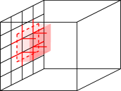
Figure 3: A $Z_{2}^{(1)}$ neutral charge, a $s$ string on the 2d boundary (red dashed loop) is created by a $Z_{2}$ membrane operator eqn. (57) in the 3d bulk (red surface). It is only neutral when on the boundary. If we translate this membrane to the bulk, there are $U_{Z_{2}}(S^{1})$ operators in the bulk that anticommute the membrane operator, justifying it as the $Z_{2}$ vortex topological excitation.

Furthermore, the 3+1D bulk has a highly non-trivial effect on the boundary: in a gapped ground state of the 2+1D model (47), one and only one of the $Z_{2}$ and $Z_{2}^{(1)}$ symmetries must be spontaneously broken. Pictorially speaking, this is because the two topological excitations with mutual statistics cannot condense simultaneously. Thus, a ground state of model (47) with the full $Z_{2}\vee Z_{2}^{(1)}$ categorical symmetry must be gapless. This is a consequence of 2+1D non-invertible gravitational anomaly Ji and Wen (2019) and the $Z_{2}\vee Z_{2}^{(1)}$ categorical symmetry characterized by 3+1D $Z_{2}$ topological order (i.e. $Z_{2}$ gauge theory).

IV The model with anomalous symmetry as the boundary of topological order in one higher dimension

Through the examples above, we have shown that a model with a finite symmetry $G$, when restricted in the symmetric sector, can be viewed as the boundary of $G$-gauge theory in one higher dimension. The conservation (the fusion rules) of the point-like gauge charge, and codimension-2 gauge flux give rise to the symmetry and algebraic higher symmetry (whose combination becomes the so-called categorical symmetry) of the $G$-symmetric model, The categorical symmetry is not spontaneously broken at the critical point of the symmetry breaking transition (see Section V for more details).

We know that a $G$-gauge theory can be twisted and becomes Dijkgraaf-Witten theory Dijkgraaf and Witten (1990). We will show that boundary of such twisted $G$-gauge theory has an anomalous $G$-symmetry. This implies that a system with anomalous $G$-symmetry’t Hooft (1980); Wen (2013) also has an algebraic higher symmetry. The combination of the two symmetries corresponds to the categorical symmetry described by the twisted $G$-gauge theory in one higher dimension. Such a system has a gapless state, where the categorical symmetry is not spontaneously broken. Also, a state with the unbroken categorical symmetry must be gapless. And the gapped states of the system must spontaneously break the anomalous $G$-symmetry.

IV.1 Boundary of double-semion model

In this section, we will study the boundary of double-semion (DS) model (i.e. the twisted $Z_{2}$ gauge theory in 2+1D) to illustrate the above result.

A 2+1D double-semion (DS) topological order has four types of excitations $\mathbf{1},s,s^{*},b$. Here $s,s^{*},f$ are topological excitations $s,s^{*}$ are semions with statistics $\pm\hskip 1.0pt\mathrm{i}\hskip 1.0pt$, and $b$ is a boson. They satisfy the following fusion relation

$$s\otimes s=\mathbf{1},\ \ s^{*}\otimes s^{*}=\mathbf{1},\ \ b\otimes b=\mathbf{1},\ \ s\otimes s^{*}=b.$$ (58)

$s$ and $s$ have a mutual $\pi$ statistics and $s$ and $s^{*}$ have a mutual boson statistics. As a result, $s$ and $b$ have a mutual $\pi$ statistics.

We consider a gapped boundary from condensing $b$ excitations. Since $b\otimes b=\mathbf{1}$ and $b$ particles have mod-2 conservation, we assume the $b$ condensation gives rise to two degenerate ground states, one with $Z_{i}=1$ and the other with $Z_{i}=-1$. The domain wall between $Z_{i}=1$ and $Z_{i}=-1$ regions corresponds a $s$ particle.

We would like to point out that, on the boundary, although $s$-type particle and $e$-type particle (in the $Z_{2}$ gauge theory discussed before) have the same fusion rule $s\otimes s=\mathbf{1}$ and $e\otimes e=\mathbf{1}$, their fusion $F$-tensor are different Freedman et al. (2004); Levin and Wen (2005). In particular, fusing three $s$-type particles into one $s$-type particle in two different ways differ by a phase $-1$:

$$[sss\to\mathbf{1}\mathbf{1}s\to\mathbf{1}s\mathbf{1}]=(-)[sss\to s\mathbf{1}\mathbf{1}\to\mathbf{1}s\mathbf{1}].$$ (59)

In contrast, fusing three $e$-type particles (described by $X_{i}=-1$) into one $e$-type particle in two different ways have the same phase:

$$[eee\to\mathbf{1}\mathbf{1}e\to\mathbf{1}e\mathbf{1}]=[eee\to e\mathbf{1}\mathbf{1}\to\mathbf{1}e\mathbf{1}]$$ (60)

For the boundary of $Z_{2}$ topological order, the above two processes of fusing $e$ particles are induced, respectively, by a pair-annihilation operator $X^{+}_{i}X^{+}_{i+1}$ and a hopping operator $X^{+}_{i}X^{-}_{i+1}+X^{-}_{i}X^{+}_{i+1}$, where

$$X^{\pm}=\frac{1}{2}(Y\pm\hskip 1.0pt\mathrm{i}\hskip 1.0ptZ).$$ (61)

Indeed, we have

$$\ \ \ \ (X^{+}_{i-1}X^{-}_{i}+X^{-}_{i-1}X^{+}_{i})(X^{+}_{i}X^{+}_{i+1})|eee\rangle$$

$$=(X^{+}_{i}X^{-}_{i+1}+X^{-}_{i}X^{+}_{i+1})(X^{+}_{i-1}X^{+}_{i})|eee\rangle.$$ (62)

The pair-annihilation operator $Z^{+}_{i}Z^{+}_{i+1}$ and hopping operator $Z^{+}_{i}Z^{-}_{i+1}+Z^{-}_{i}Z^{+}_{i+1}$ are allowed local operations, and we can use them to construct effective boundary Hamiltonian

$$H^{\text{Is}}_{P} =-\sum_{i=1}^{L}J_{1}(Z^{+}_{i}Z^{-}_{i+1}+Z^{-}_{i}Z^{+}_{i+1})+J_{2}(Z^{+}_{i}Z^{+}_{i+1}+h.c.)$$

$$\ \ \ \ \ \ \ \ \ \ \ -B\sum_{i=1}^{L}Z_{i},$$ (63)

which describes the boundary of 2+1D $Z_{2}$ topological order.

For the boundary of DS topological order, the two processes for fusing $s$ particles eqn. (59) are also induced by a pair-annihilation operator and a hopping operator. Here we choose the hopping operator to be $X_{i}-Z_{i-1}X_{i}Z_{i+1}$, which shift a domain wall from $i-\frac{1}{2}$ to $i+\frac{1}{2}$, or $i+\frac{1}{2}$ to $i-\frac{1}{2}$. The pair-annihilation or pair-creation operator is given by $Z_{i-1}(X_{i}+Z_{i-1}X_{i}Z_{i+1})$, which creates or annihilates a pair of domain walls at $i+\frac{1}{2}$ and $i-\frac{1}{2}$.

For three $s$-type particles (the domain walls) at $i-\frac{1}{2},i+\frac{1}{2},i+\frac{3}{2}$, we indeed have

$$-(X_{i+1}-Z_{i}X_{i+1}Z_{i+2})Z_{i-1}(X_{i}+Z_{i-1}X_{i}Z_{i+1})|sss\rangle$$

$$=(X_{i}-Z_{i-1}X_{i}Z_{i+1})Z_{i}(X_{i+1}+Z_{i}X_{i+1}Z_{i+2})|sss\rangle,$$ (64)

where $|sss\rangle=|\uparrow_{i-1}\downarrow_{i}\uparrow_{i+1}\downarrow_{i+2}\rangle$.

Now we can construct the boundary effective theory for the $b$ condensed boundary of DS topological order. We note that such a boundary contains a gapped excitation that corresponds to the $s$-type particle. One might expect a second boundary excitation corresponding to the $s^{*}$-type particle. However, since $b$ is condensed on the boundary, the $s$-type particle and the $s^{*}$-type particle are actually equivalent on the boundary. The simplest boundary effective lattice Hamiltonian that describes the gapped $s$ particles has a form

$$H=-B\sum_{i}Z_{i}Z_{i+1},\ \ \ \ B>0,$$ (65)

which has two degenerate ground states and the $s$ particles correspond to domain walls.

Using the above allowed local operations $X_{i}-Z_{i-1}X_{i}Z_{i+1}$ and $Z_{i-1}(X_{i}+Z_{i-1}X_{i}Z_{i+1})$, we can construct a more general boundary effective theory

$$H^{\text{DS}} =-B\sum_{i=1}^{L}Z_{i}Z_{i+1}-J_{1}\sum_{i=1}^{L}(X_{i}-Z_{i-1}X_{i}Z_{i+1})$$

$$+J_{2}\sum_{i=1}^{L}Z_{i-1}(X_{i}+Z_{i-1}X_{i}Z_{i+1}),$$ (66)

where site-$i$ and site-$(i+L)$ are identified.

We note that the above Hamiltonian is not invariant under the spin-flip transformation $\prod_{i}X_{i}$. In fact, it is invariant under a non-on-site transformation Chen et al. (2011):

$$U_{Z_{2}}=\prod_{i}X_{i}\prod_{i}s_{i,i+1},$$ (67)

where $s_{ij}$ acts on two spins as

$$s_{ij} =|\uparrow\uparrow\rangle\langle\uparrow\uparrow|+|\downarrow\uparrow\rangle\langle\downarrow\uparrow|-|\uparrow\downarrow\rangle\langle\uparrow\downarrow|+|\downarrow\downarrow\rangle\langle\downarrow\downarrow|$$

$$=\frac{1}{2}(1-Z_{i}+Z_{j}+Z_{i}Z_{j}).$$ (68)

The transformation has a simple picture: it flips all the spins and include a $(-)^{N_{\uparrow\to\downarrow}}$ phase, where $N_{\uparrow\to\downarrow}$ is the number of $\uparrow\to\downarrow$ domain wall. We see that the transformation is a $Z_{2}$ transformation (i.e. square to 1). From Appendix C, the $Z_{2}$ transformation has the following action,

$$Z_{i} \leftrightarrow-Z_{i},$$

$$X_{i} \leftrightarrow-Z_{i-1}X_{i}Z_{i+1}.$$ (69)

We find that eqn. (IV.1) is invariant under the $Z_{2}$ transformation.

From the above discussion, we see that the different fusion properties lead to different local operators. The boundary effective theories for $Z_{2}$ topological order and for the double semion topological order are different. In particular, the boundary effective theory for $Z_{2}$ topological order has an on-site $Z_{2}$ symmetry, while the boundary effective theory for the double semion topological order has a non-on-site $Z_{2}$ symmetry. The non-on-site $Z_{2}$ symmetry $U_{Z_{2}}$ implies that the model (IV.1) cannot have a gapped $Z_{2}$ symmetric ground state Chen et al. (2011).

IV.2 $\widetilde{Z}_{2}$ dual symmetry

We have seen that a 1+1D lattice model (IV.1) with an anomalous $Z_{2}$ symmetry (non-on-site symmetryChen et al. (2011); Wen (2013)) can be viewed as a boundary of twisted 2+1D $Z_{2}$ gauge theory (i.e. DS topological order). The anomalous $Z_{2}$ symmetry comes from the mod-2 conserved $b$ particles. The mod-2 conserved $s$ particles will give rise to another symmetry, which will be referred as dual $\widetilde{Z}_{2}$ symmetry. In other words, we claim that the model (IV.1) has both the $Z_{2}$ symmetry and the $\widetilde{Z}_{2}$ symmetry.

To see the $\widetilde{Z}_{2}$ symmetry explicitly, we do a dual transformation on the model (IV.1):

$$Z_{i}Z_{i+1} \to\widetilde{Z}_{i+\frac{1}{2}},$$

$$X_{i} \to\widetilde{X}_{i-\frac{1}{2}}\widetilde{X}_{i+\frac{1}{2}},$$

$$Z_{i} \to\prod_{j\leq i}\widetilde{Z}_{j-\frac{1}{2}}.$$ (70)

We find

$$\ \ \ \ X_{i}-Z_{i-1}X_{i}Z_{i+1}=X_{i}+Z_{i-1}Z_{i}X_{i}Z_{i}Z_{i+1}$$

$$\to\widetilde{X}_{i-\frac{1}{2}}\widetilde{X}_{i+\frac{1}{2}}+\widetilde{Z}_{i-\frac{1}{2}}\widetilde{X}_{i-\frac{1}{2}}\widetilde{X}_{i+\frac{1}{2}}\widetilde{Z}_{i+\frac{1}{2}}$$

$$=\widetilde{X}_{i-\frac{1}{2}}\widetilde{X}_{i+\frac{1}{2}}+\widetilde{Y}_{i-\frac{1}{2}}\widetilde{Y}_{i+\frac{1}{2}},$$ (71)

$$\ \ \ \ X_{i}+Z_{i-1}X_{i}Z_{i+1}=X_{i}-Z_{i-1}Z_{i}X_{i}Z_{i}Z_{i+1}$$

$$\to\widetilde{X}_{i-\frac{1}{2}}\widetilde{X}_{i+\frac{1}{2}}-\widetilde{Z}_{i-\frac{1}{2}}\widetilde{X}_{i-\frac{1}{2}}\widetilde{X}_{i+\frac{1}{2}}\widetilde{Z}_{i+\frac{1}{2}}$$

$$=\widetilde{X}_{i-\frac{1}{2}}\widetilde{X}_{i+\frac{1}{2}}-\widetilde{Y}_{i-\frac{1}{2}}\widetilde{Y}_{i+\frac{1}{2}}.$$ (72)

The duality transformation changes the Hamiltonian (IV.1) into:

$$\widetilde{H}^{\text{DS}}=+J_{2}\sum_{i}\prod_{j<i}\widetilde{Z}_{j-\frac{1}{2}}(\widetilde{X}_{i-\frac{1}{2}}\widetilde{X}_{i+\frac{1}{2}}-\widetilde{Y}_{i-\frac{1}{2}}\widetilde{Y}_{i+\frac{1}{2}})$$

$$\ \ \ \ -B\sum_{i}\widetilde{Z}_{i+\frac{1}{2}}-J_{1}\sum_{i}(\widetilde{X}_{i-\frac{1}{2}}\widetilde{X}_{i+\frac{1}{2}}+\widetilde{Y}_{i-\frac{1}{2}}\widetilde{Y}_{i+\frac{1}{2}}).$$ (73)

We see that the dual $\widetilde{Z}_{2}$ symmetry is generated by

$$U_{\widetilde{Z}_{2}}=\prod_{i}\widetilde{Z}_{i+\frac{1}{2}}.$$ (74)

This way, we obtain the explicit expression of the dual $\widetilde{Z}_{2}$ symmetry. The on-site $\widetilde{Z}_{2}$ symmetry $U_{\widetilde{Z}_{2}}$ implies that the model (IV.1) can have a gapped $\widetilde{Z}_{2}$ symmetric ground state, which correspond to a $Z_{2}$ symmetry breaking state.

In the dual model, $\widetilde{Z}_{i+\frac{1}{2}}=1$ describes a site with no semion $s$, while $\widetilde{Z}_{i+\frac{1}{2}}=-1$ describes a site occupied with a semion $s$. The term $\widetilde{X}_{i-\frac{1}{2}}\widetilde{X}_{i+\frac{1}{2}}+\widetilde{Y}_{i-\frac{1}{2}}\widetilde{Y}_{i+\frac{1}{2}}$ is the hopping term for the $s$ particle, while the term $\prod_{j<i}\widetilde{Z}_{j-\frac{1}{2}}(\widetilde{X}_{i-\frac{1}{2}}\widetilde{X}_{i+\frac{1}{2}}-\widetilde{Y}_{i-\frac{1}{2}}\widetilde{Y}_{i+\frac{1}{2}})$ creates a pair of $s$ particles.

V Appearance of algebraic higher symmetry at the symmetry breaking transition for general finite symmetry

In the previous section, we show the categorical symmetry in 1+1D and 2+1D models with a local degrees of freedom taking values in $Z_{2}$. In this section, we generalize the discussion to any $(n+1)$D dimensional lattice models with local degrees of freedoms taking values in any finite group $G$. Same as above, we discuss the lattice model in terms of two descriptions, generalizing the Ising model and the $Z_{2}$-link model to the $G$-matter model and the $G$-link model. A major distinction is that when $G$ is non-Abelian, the $0$-symmetry in the $G$-link model is a global symmetry that is not reduced to specifying boundary conditions. We will show the emergence of categorical symmetry at and off the critical point of Landau symmetry breaking transition in these models.

V.1 A duality point of view

$d,s$	$1,0$	$1,0$	$2,0$	$2,0$	$2,\frac{1}{3}$	$2,-\frac{1}{3}$	$3,0$	$3,\frac{1}{2}$
$\otimes$	$\bm{1}$	$a^{1}$	$a^{2}$	$b$	$b^{1}$	$b^{2}$	$c$	$c^{1}$
$\bm{1}$	$\bm{1}$	$a^{1}$	$a^{2}$	$b$	$b^{1}$	$b^{2}$	$c$	$c^{1}$
$a^{1}$	$a^{1}$	$\bm{1}$	$a^{2}$	$b$	$b^{1}$	$b^{2}$	$c^{1}$	$c$
$a^{2}$	$a^{2}$	$a^{2}$	$\bm{1}\oplus a^{1}\oplus a^{2}$	$b^{1}\oplus b^{2}$	$b\oplus b^{2}$	$b\oplus b^{1}$	$c\oplus c^{1}$	$c\oplus c^{1}$
$b$	$b$	$b$	$b^{1}\oplus b^{2}$	$\bm{1}\oplus a^{1}\oplus b$	$b^{2}\oplus a^{2}$	$b^{1}\oplus a^{2}$	$c\oplus c^{1}$	$c\oplus c^{1}$
$b^{1}$	$b^{1}$	$b^{1}$	$b\oplus b^{2}$	$b^{2}\oplus a^{2}$	$\bm{1}\oplus a^{1}\oplus b^{1}$	$b\oplus a^{2}$	$c\oplus c^{1}$	$c\oplus c^{1}$
$b^{2}$	$b^{2}$	$b^{2}$	$b\oplus b^{1}$	$b^{1}\oplus a^{2}$	$b\oplus a^{2}$	$\bm{1}\oplus a^{1}\oplus b^{2}$	$c\oplus c^{1}$	$c\oplus c^{1}$
$c$	$c$	$c^{1}$	$c\oplus c^{1}$	$c\oplus c^{1}$	$c\oplus c^{1}$	$c\oplus c^{1}$	$\bm{1}\oplus a^{2}\oplus b\oplus b^{1}\oplus b^{2}$	$a^{1}\oplus a^{2}\oplus b\oplus b^{1}\oplus b^{2}$
$c^{1}$	$c^{1}$	$c$	$c\oplus c^{1}$	$c\oplus c^{1}$	$c\oplus c^{1}$	$c\oplus c^{1}$	$a^{1}\oplus a^{2}\oplus b\oplus b^{1}\oplus b^{2}$	$\bm{1}\oplus a^{2}\oplus b\oplus b^{1}\oplus b^{2}$

Table 1: The point-like excitations and their fusion rules in 2+1D $S_{3}$ topological order. Here $b$ and $c$ correspond to pure $S_{3}$ flux excitations, $a^{1}$ and $a^{2}$ pure $S_{3}$ charge excitations, $\bm{1}$ the trivial excitation, while $b^{1}$, $b^{2}$, and $c^{1}$ are charge-flux composites. $d,s$ are the quantum dimension and the topological spin of an excitation.

We consider two lattice models defined on the triangulation of $n$-dimensional space. The vertices of the triangulation are labeled by $i$, the links labeled by $ij$, etc .

In the first model, we may call it $G$-matter model, the physical degrees of freedom live on the vertices and are labeled by group elements $g$ of a finite group $G$. The many-body Hilbert space is spanned in the following local basis

$$|\{g_{i}\}\rangle,\ \ \ g_{i}\in G.$$ (75)

The Hamiltonian is given by

$$H_{1}=-J\sum_{ij}\delta(g_{i}g_{j}^{-1})-B\sum_{i}\sum_{h\in G}L_{h}(i),$$ (76)

where

$$\delta(g)=\begin{cases}1,&\text{ if }g=1\\ 0,&\text{ otherwise }\\ \end{cases}.$$ (77)

Also, the operator $L_{h}(i)$ is given by

$$L_{h}(i)|g_{1},\cdots,g_{i},\cdots,g_{N}\rangle=|g_{1},\cdots,hg_{i},\cdots,g_{N}\rangle.$$ (78)

The Hamiltonian $H_{1}$ has an on-site $G$ 0-symmetry

$$U_{h}H_{1}=H_{1}U_{h},\ \ \ U_{h}=\prod_{i}L_{h}(i).$$ (79)

We see that when $J\gg B$, $H_{1}$ is in the symmetry breaking phase, and when $J\ll B$, $H_{1}$ is in the symmetric phase.

Our second bosonic lattice model, which we may call the $G$-link model, has degrees of freedom living on the links. On an oriented link $ij$ pointing from $i$-site to $j$ site, the degrees of freedom are labeled by $g_{ij}\in G$. The many-body Hilbert space has the following local basis

$$|\{g_{ij}\}\rangle,\ \ \ g_{ij}\in G.$$ (80)

Here, $g_{ij}$’s on links with opposite orientations satisfy

$$g_{ij}=g_{ji}^{-1}.$$ (81)

The second model is related to the first model. A state $|g_{1},\cdots,g_{i},\cdots,g_{N}\rangle$ in the first model is mapped to a state $|\cdots,g_{ij},\cdots\rangle$ in the second model where $g_{ij}=g_{i}g_{j}^{-1}$.

This connection allows us to design the Hamiltonian of the second model as

$$H_{2}= -J\sum_{ij}\delta(g_{ij})-B\sum_{i}\sum_{h\in G}Q_{h}(i)$$

$$-U\sum_{ijk}\delta(g_{ij}g_{jk}g_{ik}^{-1}),$$ (82)

where the star term $Q_{h}(i)$ acts on all the links that connect to the vertex $i$:

$$\ \ \ \ Q_{h}(i)|\cdots,g_{ij},g_{ki},g_{jk},\cdots\rangle$$

$$=|\cdots,hg_{ij},g_{ki}h^{-1},g_{jk},\cdots\rangle,$$ (83)

and the plaquette term acts as a projection to zero-flux configurations, The second model has an algebraic $(n-1)$-symmetry, denoted as $G^{(n-1)}$ Kong et al. (2020b),

$$W_{q}(S^{1})H_{2}=H_{2}W_{q}(S^{1}),~{}~{}~{}W_{q}(S^{1})={\rm Tr}\prod_{ij\in S^{1}}R_{q}(g_{ij}),$$ (84)

for any loop $S^{1}$ formed by links, where $R_{q}$ is an irreducible representation of $G$. We see that the algebraic $(n-1)$-symmetry $G^{(n-1)}$ is generated by the Wilson loop operators $W_{q}(S^{1})$, for all loops $S^{1}$ and all irreducible representations $q$. We note that the algebraic $0$-symmetry $G^{(0)}$ is different from the usual 0-symmetry characterized by a group $G$, when $G$ is non-Abelian. But when $G$ is Abelian the algebraic $0$-symmetry $G^{(0)}$ happen to be the usual 0-symmetry $G$. Also, for Abelian $G$, $G^{(n)}$ is a $n$-symmetry described by a higher group. But, for non-Abelian $G$, $G^{(n)}$ is an algebraic $n$-symmetry beyond higher group.

The Hamiltonian $H_{2}$ has the algebraic $(n-1)$-symmetry, because $Q_{h}(i)$ term in the Hamiltonian can be viewed as a “gauge” transformation and the Wilson loop operator $W_{q}(S^{1})$ is gauge invariant, and hence

$$W_{q}(S^{1})Q_{h}(i)=Q_{h}(i)W_{q}(S^{1}).$$ (85)

$W_{q}(S^{1})$ commutes with other terms in $H_{2}$ since they are all diagonal in the $|\{g_{ij}\}\rangle$ basis.

In the limit $|B|\ll J\ll U$, the ground state of $H_{2}$ is a trivial product state

$$|\{g_{ij}=1\}\rangle,$$ (86)

which is symmetric under the algebraic $(n-1)$ symmetry $G^{(n-1)}$. In the other limit $|J|\ll B\ll U$, the ground state of $H_{2}$ is a topologically ordered state (described by the $G$-gauge theory), breaking the algebraic $(n-1)$ symmetry $G^{(n-1)}$ spontaneously.

What is the global $G$ symmetry operator in the first model eqn. (79) mapped to? It is mapped to a global $0$-symmetry operator,

$$\mathcal{U}_{h}H_{2}=H_{2}\,\mathcal{U}_{h},\ \ \ \mathcal{U}_{h}=\prod_{i}Q_{h}(i)\,.$$ (87)

In particular, when the model has periodic boundary condition, this $0$-symmetry acts as $\mathcal{U}_{h}|g_{ij}\rangle=|hg_{ij}h^{-1}\rangle$. Thus the global symmetry is an inner automorphism of $G$, denoted as $\operatorname{Inn}(G)$. When the centralizer of $G$ is trivial, $\operatorname{Inn}(G)\cong G$.

Only when $G$ is Abelian, the global symmetry action in (87) reduces to claiming the boundary conditions or the twisted sectors of the model. For example, when $G=Z_{2}$ and $d=1$, it reduces to $U_{\widetilde{Z}_{2}}$ in (11).

Furthermore, the symmetry generators of the algebraic $(n-1)$-symmetry $G^{(n-1)}$ and the $0$-symmetry $\operatorname{Inn}(G)$ commute,

$$W_{q}(S^{1})\,\mathcal{U}_{h}=\mathcal{U}_{h}W_{q}(S^{1})\,.$$ (88)

In the limit $U\to+\infty$, the low energy part of $H_{2}$ can be mapped to $H_{1}$ via the following duality and inverse duality map,

$$g_{ij} =g_{i}g_{j}^{-1}, \left(g_{i_{0}}\right)^{-1}g_{i} =\left(g_{i_{0}j}g_{jk}\cdots g_{li}\right)^{-1},$$ (89)

where $i_{0}$ is a fixed base point. Note that to map a configuration $g_{i}$ to a configuration $g_{ij}$, we need to pick a base point $i_{0}$ and a value $g_{i_{0}}$. Therefore, the above map is a $|G|$-to-one map. It maps the following $|G|$ configurations of $H_{1}$ (label by $h\in G$), $|\{hg_{i}\}\rangle$, into the same configuration configuration of $H_{2}$, $|\{g_{ij}\}\rangle$. Thus the spectrum of $H_{1}$ formed by $G$ invariant states, $|\Psi\rangle=U_{h}|\Psi\rangle$, is identical to the low energy spectrum of $H_{2}$ below $U$. $H_{1}$ and $H_{2}$ have the same $G$-symmetric low energy dynamics. In particular they have the same phase transition and critical point.

The $G$-symmetry breaking phase of $H_{1}$ corresponds to the trivial phase of $H_{2}$ (which is the symmetric phase of the algebraic $(n-1)$-symmetry $G^{(n-1)}$) and the $G$-symmetric phase of $H_{1}$ corresponds to the topologically ordered phase of $H_{2}$ (which is the symmetry breaking phase of the algebraic $(n-1)$-symmetry $G^{(n-1)}$) Gaiotto et al. (2015); Kong et al. (2020b). Now we see that the critical point at the symmetry breaking transition neighbors a phase with $G$ 0-symmetry and a phase with algebraic $(n-1)$-symmetry. Heuristically, the emergent symmetry at the critical point is the same or larger than the neighboring gapped phases. Thus the critical point has both the $G$ 0-symmetry and the algebraic $(n-1)$-symmetry $G^{(n-1)}$. In other words, the critical point has a categorical symmetry $G\vee G^{(n-1)}$ which is the combination of the $G$ 0-symmetry and the algebraic $(n-1)$-symmetry $G^{(n-1)}$.

V.2 Patch symmetry operators

Now let us discuss the charges of the categorical symmetry in the model given by the previous two descriptions. Just as the case $G=Z_{2}$ discussed before, we can only create neutral charges, by patch operators. The $0$-symmetry patch operator creates conserved charges of $(n-1)$-symmetry, part of the conserved charges can be measured by the $(n-1)$-symmetry patch operator, and vice versa.

We start with the simple case that $n=1$. For a generic group, one set of patch operators, from site $i_{1}$ to site $i_{2}$, acting on a state $|\{g_{ij}\}\rangle$, are

$$W_{q,\alpha\beta}(i_{1},i_{2})=\left(\prod_{i=i_{1}}^{i_{2}}R_{q}(g_{ij})\right)_{\alpha\beta}\,,$$ (90)

where $\alpha,\beta$ runs from $1$ to $n_{R}$, the dimension of the irreducible representation $R_{q}$ of $G$. The other set of patch operators are

$$\mathcal{U}_{h}(i_{1},i_{2})=\prod_{i=i_{1}}^{i_{2}}Q_{h}(i)\,.$$ (91)

They satisfy the following commutation relations with the ordering $i_{1}<i_{2}<i_{3}<i_{4}$, and a simplified notation $W_{q}(i_{1},i_{3})=W_{q,13},\,\mathcal{U}_{h}(i_{2},i_{4})=\mathcal{U}_{h,24}$, (with the subscript $\alpha,\beta$ of $W_{q}(l_{1},l_{2})$ suppressed),

$$\begin{split}{\rm Tr}\left[W_{q,13}\;\mathcal{U}_{h,24}\,(W_{q,13})^{\dagger}\right]=&\,\chi^{q}(h^{-1})\,\mathcal{U}_{h,24}\,,\\ {\rm Tr}\left[(W_{q,13})^{\dagger}\;\mathcal{U}_{q,24}\,W_{q,13}\right]=&\,\chi^{q}(h)\,\mathcal{U}_{h,24}\,,\\ {\rm Tr}\left[(W_{q,24})\;\mathcal{U}_{h,13}\,(W_{q,24})^{\dagger}\right]=&\,\chi^{q}(h)\,\mathcal{U}_{h,13}\,,\\ {\rm Tr}\left[(W_{q,24})^{\dagger}\;\mathcal{U}_{h,13}\,W_{q,24}\right]=&\,\chi^{q}(h^{-1})\,\mathcal{U}_{h,13}\,.\end{split}$$ (92)

where $\chi^{q}(h)$ is the character of $h$ in the $q$ representation. The character represents that the $0$-symmetry charge and the algebraic $(n-1)$-symmetry charge are mutually non-local.

More generally, for any $n$, the patch operator that creates the neutral charge for dual $(n-1)$-symmetry $G^{(n-1)}$ is defined on a $n$-dimensional patch (disk), $D^{n}$, and is given by the product of star terms,

$$\mathcal{U}_{h}(D^{n})=\prod_{i\in D^{n}}Q_{h}(i).$$ (93)

The $G^{(n-1)}$ neutral charge lives on the boundary of $D^{n}$, denoted as $(S^{n-1})^{\vee}$, living on the dual lattice. Let us call it $s$. In particular, when $G$ is Abelian, $\mathcal{U}_{h}(D^{n})$ acts trivially inside $D^{n}$. That is $\mathcal{U}_{h}$ is in fact defined on the boundary of $D^{n}$,

$$\mathcal{U}_{h}[(S^{n-1})^{\vee}]= \prod_{ij\in(S^{n-1})^{\vee}}T_{h}(ij),$$ (94)

$$T_{h}(ij)|g_{ij}\rangle= \begin{cases}|hg_{ij}\rangle&i\in D^{n}\\ |g_{ij}h^{-1}\rangle&j\in D^{n}\\ \end{cases}.$$ (95)

For $G=Z_{2}$ and $d=2$, we recover the $s$ string operator eqn. (53).

The other patch operator that creates conserved charges for the 0-symmetry $G$ is $W_{q}(C_{ij})$ defined on any open string $C_{ij}$. The $0$-symmetry charges are at the end points $i$ and $j$ sites of the open string. Let us call them $e$ particles.

These charges can be thought of as the topological excitations in $(n+1)$D topological orderKong and Wen (2014); Lan et al. (2018); Lan and Wen (2019); Gaiotto and Johnson-Freyd (2019); Johnson-Freyd (2020). The $e$ particle corresponds to the point-like topological excitations, and the $s$ corresponds to the other topological excitations on the closed $(S^{n-1})^{\vee}$ surface. For example, when $d=2$, and $G=Z_{2}$, $\mathcal{U}_{h}\left[(S^{1})^{\vee}\right]$ is the closed $Z_{2}$ vortex string operator. This conserved charge of $\widetilde{Z}_{2}^{(1)}$ can be thought of as coming from the topological string excitation in $3+1$-dimensional $Z_{2}$ topological field theory, as discussed in section III and illustrated in Fig. 3.

V.3 An example of algebraic $1$-symmetry $S_{3}^{(1)}$ in $2+1$D theories

The simplest example where the algebraic symmetry is beyond a higher symmetry is in the $(n+1)$D model (V.1) with $d=2$ and $G=S_{3}$. Here, $S_{3}=\langle s,r|s^{3}=r^{2}=1,rsr=s^{2}\rangle$ is the permutation group on $3$ elements. The topologically ordered phase of (V.1) is described by $S_{3}$ gauge theory. There are $8$ types of anyonic excitations in the model. Their fusion rules are shown in Table 1.

The model (V.1) has an algebraic 1-symmetry, which denoted as $S_{3}^{(1)}$. The generators are two Wilson line operators (see eqn. (84)), labeled by the two non-trivial irreducible representations $a^{1}$ and $a^{2}$ of $S_{3}$. The end of Wilson line operators create anyons $a^{1}$ and $a^{2}$ whose fusion is descrined in Table 1. The product of Wilson line operators is given by the fusion of irreducible representations (i.e. the fusion of the anyons $a^{1}$ and $a^{2}$):

$$\begin{split}&W^{a^{1}}(S^{1})W^{a^{1}}(S^{1})=\mathbf{1},\\ &W^{a^{2}}(S^{1})W^{a^{2}}(S^{1})=\mathbf{1}+W^{a^{1}}(S^{1})+W^{a^{2}}(S^{1}),\\ &W^{a^{1}}(S^{1})W^{a^{2}}(S^{1})=W^{a^{2}}(S^{1}).\end{split}$$ (96)

The product of two $W^{a^{2}}(S^{1})$’s reveals that the symmetry is an algebraic $(n-1)$-symmetry beyond higher group. In general, if $G$ is non-Abelian, $G^{(n-1)}$ is an algebraic $(n-1)$-symmetry beyond higher group.

V.4 A holographic point of view

Figure 4: The conservation (the fusion rule) of the $Z_{2}$ point-like charge and $\widetilde{Z}^{(1)}_{2}$ loop-like flux in the 3+1D $Z_{2}$ gauge theory give rise to the categorical symmetry of the 2+1D lattice model $H_{1}$ (76). The mod-2 conservation of $Z_{2}$ charge $e$ gives rise to the $Z_{2}$ 0-symmetry. The mod-2 conservation of $Z_{2}^{(1)}$ flux $s$ gives rise to the $Z_{2}^{(1)}$ 1-symmetry. $e$ and $s$ has a mutual $\pi$ statistics between them.

Let us start with the lattice model $H_{1}$ (76) with a finite 0-symmetry $G$. We would like to study the $G$-symmetry within the restricted symmetric sub-Hilbert space. In the symmetric sub-Hilbert space, the $G$-symmetry transformation (79) will be trivial. It appears that we cannot see the $G$-symmetry. But we can see the $G$-symmetry via point-like excitations in a finite region, which carry non-trivial representations of $G$. The non-trivial fusion of $G$-representations (in particular, the fusion channel of nontrivial representations into a trivial representation) signifies the $G$ 0-symmetry in the symmetric sub-Hilbert space. Thus, restricting to the symmetric sub-Hilbert space forces us to view the $G$-symmetry via the fusion category of the symmetry charges. This is the categorical view of symmetry.Lan et al. (2017)

The lattice model $H_{1}$ (76), when restricted to the symmetric sub-Hilbert space, has a gravitational anomaly. This is because the symmetric sub-Hilbert space ${\cal V}_{\text{symm}}$ does not have a tensor product decomposition ${\cal V}_{\text{symm}}\neq\otimes_{i}{\cal V}_{i}$, in terms of the local Hilbert space ${\cal V}_{i}$ on each site. This suggests that the fusion category of the symmetry charges is anomalous,Wen (2013); Kong and Wen (2014) i.e. the fusion category can only be realized at a boundary of a topological order in one higher dimension. Indeed, the model $H_{1}$ (76), when restricted to the symmetric sub-Hilbert space, can be viewed as a boundary of $G$-gauge theory in one higher dimension, where a simple example is discussed in Section II.4.Ji and Wen (2019) The gauge charges in the $G$-gauge theory also carry representations of $G$. The non-trivial fusion of $G$-representations give rise to the $G$ 0-symmetry both in the bulk and at the boundary. This is how the finite 0-symmetry $G$ in the model $H_{1}$ (76) appears via the $G$-gauge theory in one higher dimension.

But the $G$-gauge theory also has other excitations (such as the gauge flux – codimension-2 excitations), which also fuse in a non-trivial way and give rise to additional symmetry to the lattice model $H_{1}$ (76). So the complete symmetry of the lattice model $H_{1}$ (76) is given by the non-trivial fusion of all the excitations (see Fig. 4). Such a complete symmetry is called categorical symmetry of the lattice model $H_{1}$ (76) (when restricted to the symmetric sub-Hilbert space). The categorical symmetry is fully characterized by the $G$-gauge theory in one higher dimension. The data in one higher dimension includes gauge charges, gauge fluxes, their fusion rules, and the mutually non-local property. The set of data realizes on the boundary as the global symmetry charges, the global algebraic higher symmetry charges, their fusion as well as their mutual statistics. This is the holographic understanding of the categorical symmetry. Compare to our patch-operator understanding of the categorical symmetry discussed in Sections II.2 and V.2, holographic view reveals the essence of the categorical symmetry more clearly.

Let us rephase the above holographic point of view using a categorical language (for details see LABEL:KZ200514178 and Appendix A). The braiding and fusion of the particles carrying $G$ representations is described by the fusion $n$-category $n{{\cal R}\text{ep}}(G)$. Every fusion higher category can be mapped into a braided fusion higher category by a $Z_{1}$ functor, called $Z_{1}$ center in this paper (see eqn. (102), and, for a physical description, see for example LABEL:KZ200514178). The $Z_{1}$ center of the fusion $n$-category $n{{\cal R}\text{ep}}(G)$ is denoted as $Z_{1}(n{{\cal R}\text{ep}}(G))$, which is a braided fusion $n$-category. In fact, $Z_{1}(n{{\cal R}\text{ep}}(G))$ describes the excitations in the $G$-gauge theory in one higher dimension (i.e. in $(d+2)$-dimensional spacetime) and is denoted as $\mathcal{G}^{d}_{G}$. In other words, $\mathcal{G}^{d}_{G}=Z_{1}(n{{\cal R}\text{ep}}(G))$Freed and Teleman (2018); Kong et al. (2020b).

Therefore, for a system with symmetry described by a fusion $n$-category $n{{\cal R}\text{ep}}(G)$ (which is nothing but the $G$ 0-symmetry), to find its categorical symmetry is to find the $Z_{1}$ center of $n{{\cal R}\text{ep}}(G)$: $Z_{1}(n{{\cal R}\text{ep}}(G))$. $Z_{1}(n{{\cal R}\text{ep}}(G))$ describes the excitations in the $G$-gauge theory in one higher dimension. This is the holographic point of view of the categorical symmetry.

We stress that the lattice model $H_{1}$ (76) (when restricted to the symmetric sub-Hilbert space) has the full categorical symmetry, but its ground states may spontaneously break part of the categorical symmetry. Those different ground states correspond to different boundaries of the $G$-gauge theory. Since a gapped boundary of $G$-gauge theory always comes from condensation of gauge charges, or gauge flux, or some combinations of them, a gapped boundary always spontaneously breaks some part of the categorical symmetry. Therefore, the gapped ground states of $H_{1}$ always spontaneously break some part of the categorical symmetry. Because the gauge charge and gauge flux have non-trivial mutual statistics between them, we cannot condense all gauge charges and gauge fluxes simultaneously. Therefore, any ground states of the lattice model $H_{1}$ (76) cannot break the categorical symmetry completely.

The $G$-gauge theory has a gapless boundary if none of the gauge charges and gauge flux is condensed. Such a boundary does not break the categorical symmetry. Thus the lattice model $H_{1}$ (76) has a gapless ground state where the categorical symmetry is not spontaneously broken. This gapless state should correspond to the critical point of the Landau $G$-symmetry breaking transition. The above discussions also apply to the dual model $H_{2}$ (V.1).

VI The emergence of algebraic higher symmetry

We have seen that a $G$ 0-symmetry in $n$-dimensional space can be fully characterized by a fusion $n$-category $n{{\cal R}\text{ep}}(G)$, describing the fusion of the charge objects of the $G$-symmetry. In fact, the charge objects described by $n{{\cal R}\text{ep}}(G)$ are nothing but the excitations on top of a product state with the $G$-symmetry. To be precise, $n{{\cal R}\text{ep}}(G)$ describes the types of the excitations, which are the equivalence classes under the $G$-symmetry preserving deformations (i.e. two excitations are equivalent if they can deform into each other smoothly without breaking the symmetry). This is why $n{{\cal R}\text{ep}}(G)$ depends on the symmetry $G$, despite it describes excitations in a trivial product state.

Similarly, the algebraic $(n-1)$-symmetry $G^{(n-1)}$ in the lattice model eqn. (V.1) is fully characterized by a fusion $n$-category $n{{\cal V}\text{ec}}_{G}$, describing the fusion of the charge objects of the $G^{(n-1)}$-symmetry. Again, $n{{\cal V}\text{ec}}_{G}$ describe the types of the excitations on top of a product state with the $G^{(n-1)}$-symmetry. Now types are the equivalence classes under the $G^{(n-1)}$-symmetry preserving deformations.

This result can be generalized. Consider a lattice model with an algebraic higher symmetry in $n$-dimensional space, which has a symmetric product state as its ground state (such as eqn. (86)). The types of the excitations on top of the product state is described by a fusion $n$-category ${\cal R}$, and the algebraic higher symmetry is fully characterized by ${\cal R}$. So we will refer an algebraic higher symmetry as ${\cal R}$.

We would like to remark that the fusion higher category ${\cal R}$ describe excitations on top of a product state is a special class of fusion higher category , called the local fusion higher category. Actually, describing types of excitations on top of a symmetric product state is the defining property of local fusion higher category. We believe that local fusion $n$-categories classify algebraic higher symmetries in $n$-dimensional space.Kong et al. (2020b)

Now, let us consider a lattice theory or a field theory in $n$-dimensional space, whose low energy excitations happen to be described by a local fusion $n$-category ${\cal R}$. If we ignore all the high energy excitations and pretend ${\cal R}$ are only excitations, then we can pretend ${\cal R}$ to be the excitations in a product state with the algebraic higher symmetry ${\cal R}$. In this way, we say that the theory has an emergent algebraic higher symmetry ${\cal R}$, and we can regard the system to be in a trivial ${\cal R}$-symmetric phase.

Let us elaborate with some examples of emergent algebraic higher symmetries. The first is the model with a finite 0-symmetry $G$ in $n$-dimensional space, which we now discuss using the point of view of local fusion higher category. If the ground state of the model is a product state with $G$ symmetry, then the excitations will be point-like and are labeled by the irreducible representations of $G$. Those excitations are described by a local fusion $n$-category $n{{\cal R}\text{ep}}(G)$. Thus the $G$ 0-symmetry can also be denoted as $n{{\cal R}\text{ep}}(G)$ symmetry. If the model is in the spontaneous symmetry breaking phase, the ground states will be degenerate and are labeled by the ground elements $g\in G$. The excitations will be $(n-1)$-dimensional domain walls between different degenerate ground states. Those domain wall excitations are labeled by pairs $(g_{1},g_{2})$ if the domain wall connect the ground state $g_{1}$ and the ground state $g_{2}$. Under a symmetry transformation $g\in G$, the domain wall transform as $(g_{1},g_{2})\to(gg_{1},gg_{1})$. We say $(g_{1},g_{2})$ and $(gg_{1},gg_{1})$ are equivalent. The equivalent classes of domain walls (i.e. symmetrized domain walls) are labeled by a single group element $h=g_{1}^{-1}g_{2}$. Those excitations are described by a fusion $n$-category $n{{\cal V}\text{ec}}_{G}$. It turns out that $n{{\cal V}\text{ec}}_{G}$ is also a local fusion $n$-category.Kong et al. (2020b) The algebraic higher symmetry $n{{\cal V}\text{ec}}_{G}$ is nothing but the algebraic $(n-1)$-symmetry $G^{(n-1)}$ generated by Wilson loop operators that we discussed before.

The second example of 2d lattice model has $S_{3}=Z_{3}\rtimes Z_{2}$ $0$-symmetry. We have a phase with $S_{3}$ 0-symmetry. We have another phase that spontaneously breaks the $S_{3}$ 0-symmetry. This phase has an emergent $S_{3}^{(1)}$ algebraic $1$-symmetry. We also have some other phases that break different symmetries, and thus have different emergent algebraic higher symmetries. All those phases and their emergent algebraic higher symmetries are listed below:

• $S_{3}$ symmetric phase, whose point-like charges are

  $${\cal R}_{S_{3}}=2{{\cal R}\text{ep}}(S_{3})=\{\mathbf{1},p_{1},p_{2}\}.$$ (97)

• $Z_{2}$ (charge conjugation) spontaneous symmetry breaking phase with $Z_{3}$ symmetry, whose point-like and string-like excitations are

  $${\cal R}_{Z_{3},Z_{2}^{(1)}}=\{\mathbf{1},p,\bar{p},s\}.$$ (98)

  which include $Z_{3}$ charges $p,\bar{p}$ (point-like) and $Z_{2}$ domain wall $s$ (string-like).

• $Z_{3}$ spontaneous symmetry breaking phase with $Z_{2}$ symmetry:

  $${\cal R}_{Z_{2},Z_{3}^{(1)}}=\{\mathbf{1},p,s,\bar{s}\}.$$ (99)

  which include $Z_{2}$ charge $p$ (point-like) and $Z_{3}$ domain wall $s,\bar{s}$ (string-like).

• $S_{3}$ spontaneous symmetry breaking phase, whose string-like excitations are labeled group elements

  $${\cal R}_{S_{3}^{(1)}}=2{{\cal V}\text{ec}}_{S_{3}}=\{s_{h}|h\in G\}.$$ (100)

${\cal R}_{S_{3}}=2{{\cal R}\text{ep}}(S_{3})$ and ${\cal R}_{S_{3}^{(1)}}=2{{\cal V}\text{ec}}_{S_{3}}$ are local fusion 2-categories, since they describe excitations on top of symmetric product states, as explicilty shown in Section V. They correspond to algebraic higher symmetries: the 0-symmetry $S_{3}$ and the algebraic 1-symmetry $S_{3}^{(1)}$. Using the results in LABEL:KZ200514178, we find that ${\cal R}_{Z_{2},Z_{3}^{(1)}}$ and ${\cal R}_{Z_{3},Z_{2}^{(1)}}$ are also local fusion 2-categories, and they also correspond to two algebraic higher symmetries. The algebraic higher symmetry ${\cal R}_{Z_{2},Z_{3}^{(1)}}$ contains a 0-symmetry $Z_{2}$ (the conservation of the $Z_{2}$ charges) and a 1-symmetry $Z_{3}^{(1)}$ (the conservation of the $Z_{3}$ domain walls). The algebraic higher symmetry ${\cal R}_{Z_{3},Z_{2}^{(1)}}$ contains a 0-symmetry $Z_{3}$ (the conservation of the $Z_{3}$ charges) and a 1-symmetry $Z_{2}^{(1)}$ (the conservation of the $Z_{2}$ domain walls).

Those four algebraic higher symmetries form two dual pairs: $(2{{\cal R}\text{ep}}(S_{3}),2{{\cal V}\text{ec}}_{S_{3}})$ and $({\cal R}_{Z_{2},Z_{3}^{(1)}},{\cal R}_{Z_{3},Z_{2}^{(1)}})$. Moreover, the $Z_{1}$ center of all above ${\cal R}$’s is the same $Z_{1}({\cal R})=\mathcal{G}^{2}_{S_{3}}$, the same category that describes the topological data of $3$d $S_{3}$ topological order, which characterizes the $S_{3}\vee S_{3}^{(1)}$ categorical symmetry.

In fact, all the four phases discussed above have the same emergent categorical symmetry $S_{3}\vee S_{3}^{(1)}$. But in different phases, the categorical symmetry is spontaneously broken in different ways. It turns out that, to understand the emergent algebraic higher symmetry, it is better to understand the emergent categorical symmetry first. Then, the emergent algebraic higher symmetry is just the unbroken part of the emergent categorical symmetry. In the next section, we use this point of view to understand the emergent categorical symmetry and emergent algebraic higher symmetry in a more general setting.

VII The emergence of categorical symmetry (and algebraic higher symmetry)

In this section, we consider a lattice theory or a field theory in $n$-dimensional space, whose low energy excitations are described by a fusion $n$-category ${\cal C}$. Some excitations in ${\cal C}$ may correspond to charge objects of a certain symmetry, and other excitations correspond topological excitations not associated with symmetry. Here we ignore all the high energy excitations and pretend ${\cal C}$ are the only excitations. Moreover, we use the categorical point of view of symmetry, i.e. we view all the charge objects as topological excitations, and ignore their symmetry origin. This is possible since the symmetry is fully encoded in the fusion of the charge objects. Now, we would like to ask: what is the emergent algebraic higher symmetry in a theory with low energy excitations ${\cal C}$? First we would like to understand what is the emergent categorical symmetry in a theory with low energy excitations ${\cal C}$.

Let us consider an example of 2+1D product state with a $Z_{2}$-symmetry. The state has point-like excitations ${\cal C}_{Z_{2}\text{-sym}}=\{\mathbf{1},e\}$, where $\mathbf{1}$ has $Z_{2}$ charge-0, and $e$ has $Z_{2}$ charge-1. Since the Hamiltonian has $Z_{2}$ symmetry, ${\cal C}_{Z_{2}\text{-sym}}=\{\mathbf{1},e\}$ should give rise to the $Z_{2}$ symmetry. The second example is the $Z_{2}$ topological order (described by $Z_{2}$ gauge theory) without any symmetry. The topological phase has point-like excitations ${\cal C}_{Z_{2}\text{-top}}=\{\mathbf{1},e,m,f\}$. Since the Hamiltonian has no symmetry, ${\cal C}_{Z_{2}\text{-top}}=\{\mathbf{1},e,m,f\}$ should not give rise to any symmetry.

When viewed as two fusion 2-categories describing topological excitations in 2d topological orders, why ${\cal C}_{Z_{2}\text{-sym}}$ give rise to symmetry while ${\cal C}_{Z_{2}\text{-top}}$ gives rise to no symmetry? To see their difference, here we would like to introduce the notion of gravitational anomaly. Conventionally, the gravitational anomaly refers to a non-invariance of the path integral measure under the diffeomorphism transformations of spacetime manifold. Here, following LABEL:W1313,KW1458, we define gravitational anomaly differently, as the obstruction to regularize the theory by a local lattice bosonic model without symmetry in the same dimension. We ask whether there exists a local lattice bosonic model without symmetry in the same dimension, whose complete excitations reproduce the fusion category ${\cal C}$. If such a lattice model exist, then the fusion category ${\cal C}$ is free of gravitational anomaly. If the lattice regularization without symmetry does not exist, then the fusion category ${\cal C}$ has a gravitational anomaly. It turns out that ${\cal C}_{Z_{2}\text{-top}}$ has no gravitational anomaly, while ${\cal C}_{Z_{2}\text{-sym}}$ has a gravitational anomaly. One may say that ${\cal C}_{Z_{2}\text{-sym}}$ can be realize as excitations in a lattice model, and should be anomaly-free. However, the lattice regularization of ${\cal C}_{Z_{2}\text{-sym}}$ requires a $Z_{2}$ symmetry. ${\cal C}_{Z_{2}\text{-sym}}$ has no lattice regularization without symmetry, and thus has a gravitational anomaly.

The above examples reveals a general property: if the excitations are described by anomaly-free fusion higher category ${\cal C}$, then there is no emergent symmetry. Here, the emergent symmetries are global symmetries that can be beyond group-like. If ${\cal C}$ is anomalous, then there is an emergent symmetry. We see that emergent symmetry $\sim$ gravitational anomaly. So to understand emergent symmetry, we need to understand gravitational anomaly.

But in the above, we just defined what is “no gravitational anomaly” as the existence of lattice regularization in the same dimension. We did not define what is gravitational anomaly. To define what is gravitational anomaly, we rely on the following conjecture, the holographic principle of topological order:Kong and Wen (2014); Kong et al. (2015, 2017) The excitations in $n$-dimensional space described by a fusion $n$-category ${\cal C}$ can always be realized at a boundary of an anomaly-free topological order (denoted as $\mathsf{M}$) in one higher dimensions. Moreover, the topological order $\mathsf{M}$ is uniquely determined by ${\cal C}$, we denote this map from ${\cal C}$ and $\mathsf{M}$ as $\mathsf{M}=\mathsf{bulk}({\cal C})$. Using the holographic principle, we can rephrase the anomaly-free condition for a fusion higher category ${\cal C}$ as

$$\mathsf{bulk}({\cal C})=\mathbf{1},$$ (101)

where $\mathbf{1}$ denotes the trivial topological order (i.e. a product state with no symmetry). This is because if ${\cal C}$ can be realized by a boundary of a product state in a lattice model in one higher dimension, we can always remove the bulk product state, and conclude that ${\cal C}$ can be realized by a lattice model in the same dimension. Thus the holographic principle can tell us when there exists a gravitational anomaly. Furthermore, the holographic principle gives a way to regularize the anomalous theory ${\cal C}$ on a $n+1$ dimensional lattice, ${\cal C}$ is realized as one low energy phase of a boundary of the lattice model. Thus the holographic principle tells us what is gravitational anomaly: a gravitational anomaly is a topological order in one higher dimension.Kong and Wen (2014); Kong et al. (2015, 2017)

Should we view the bulk topological order $\mathsf{M}$ (the gravitational anomaly) as the emergent symmetry? May be not. The emergent symmetry should be related to conservation laws encoded by fusion rules, or more precisely a fusion higher category. In fact, from the bulk topological order $\mathsf{M}$ in $(n+1)$-dimensional space, we can get a fusion $(n+1)$-category ${\cal M}$ describing its excitations. Since the bulk topological order $\mathsf{M}$ is anomaly-free all the codimension-1 excitations are descendent (i.e. formed by codimension-2 and higher excitations). We can drop the codimension-1 excitations, which turns the fusion $(n+1)$-category ${\cal M}$ into a braided fusion $n$-category $\mathcal{M}$. This turns the map from ${\cal C}$ to $\mathsf{M}$, $\mathsf{M}=\mathsf{bulk}({\cal C})$, into a map from ${\cal C}$ to $\mathcal{M}$:

$$\mathcal{M}=Z_{1}({\cal C}).$$ (102)

So we should view the braided fusion $n$-category $\mathcal{M}$ as the emergent symmetry ${\cal C}$. Since $\mathcal{M}$ describes the excitations in a topological order in one higher dimension where ${\cal C}$ is realized as a boundary, we see that $\mathcal{M}$ is actually the emergent categorical symmetry.

Now, we can say that the fusion 2-category ${\cal C}_{Z_{2}\text{-top}}=\{\mathbf{1},e,m,f\}$ that describes the excitations in the 2+1D $Z_{2}$ topological order has no emergent categorical symmetry since $Z_{1}({\cal C}_{Z_{2}\text{-top}})=\{\mathbf{1}\}$. Similarly, the fusion 2-category ${\cal C}_{0}=\{\mathbf{1}\}$ that describes the excitations in the 2+1D product state with no symmetry has no emergent categorical symmetry since $Z_{1}({\cal C}_{0})=\{\mathbf{1}\}$. Since the both phases have no categorical symmetry. We can find a lattice model with no symmetry in which the above two phases can transform into each other via phase transitions. As there is no global symmetry to be concerned, we just turn off the Hamiltonian for $Z_{2}$ topological order and turn on another for the product state.

On the other hand, the fusion 2-category ${\cal C}_{Z_{2}\text{-sym}}=\{\mathbf{1},e\}$ that describes the excitations in the 2+1D $Z_{2}$-symmetric product state has an emergent categorical symmetry described by $Z_{1}({\cal C}_{Z_{2}\text{-sym}})$. In fact, $Z_{1}({\cal C}_{Z_{2}\text{-sym}})$ is the braided fusion $2$-category (denoted as $\mathcal{G}^{2}_{Z_{2}}$) describing the excitations in a 3+1D $Z_{2}$ gauge theory. Therefore, ${\cal C}_{Z_{2}\text{-sym}}=\{\mathbf{1},e\}$ has an emergent categorical symmetry $\mathcal{G}^{2}_{Z_{2}}=Z_{1}({\cal C}_{Z_{2}\text{-sym}})$. In this case, we cannot connect a phase described by the fusion 2-category ${\cal C}_{Z_{2}\text{-sym}}=\{\mathbf{1},e\}$ to a phase described by the fusion 2-category ${\cal C}_{0}=\{\mathbf{1}\}$.

The above result sounds counter-intuitive, since ${\cal C}_{Z_{2}\text{-sym}}=\{\mathbf{1},e\}$ can be realized by a $Z_{2}$-symmetric product state and ${\cal C}_{0}=\{\mathbf{1}\}$ can be realized by a product state with no symmetry. Two product states should be in the same phase and are connected by phase transitions (actually connected by zero phase transition). When we say $Z_{2}$-symmetric product state, we also specify the deformation class of the Hamiltonians, which are all required to have the $Z_{2}$-symmetry. In the phase diagram of the $Z_{2}$-symmetric Hamiltonians, there is no phase whose excitations are given by ${\cal C}_{0}=\{\mathbf{1}\}$, but there is a phase whose excitations are given by ${\cal C}_{Z_{2}\text{-sym}}=\{\mathbf{1},e\}$. This is what we mean by “a phase described by the fusion 2-category ${\cal C}_{Z_{2}\text{-sym}}=\{\mathbf{1},e\}$ is not connected to a phase described by the fusion 2-category ${\cal C}_{0}=\{\mathbf{1}\}$”. In general, if low energy excitations ${\cal C}$ has non-trivial categorical symmetry $Z_{1}({\cal C})$, then any gapped phase formed by condensing those low energy excitations cannot be a trivial phase with excitation $\{\mathbf{1}\}$. This comes from the knowledge that $Z_{1}({\cal C})\neq Z_{1}(\{\mathbf{1}\})$.

We see that the emergent categorical symmetry can constrain the possible phases and phase transitions, just like the usual symmetry does. This represents one of the most important application of categorical symmetry (see Section VII.1).

Let us discuss more examples of emergent categorical symmetry using the 2+1D $Z_{2}$ topological order.Read and Sachdev (1991); Wen (1991) The $Z_{2}$-topological order has a trivial excitation $\mathbf{1}$ and three non-trivial excitations $e,\ m,\ f$ with mod 2 conservation. $e,\ m$ are bosons and $f$ is a fermion, and they fuse as $e\otimes m=f$. If the low energy excitations are ${\cal R}=\{\mathbf{1},e\}$ (and $m,f$ are assume to have very high energies), then ${\cal R}$ is a local fusion $2$-category ${\cal R}=2{{\cal R}\text{ep}}(Z_{2})$, which describes an anomaly-free $Z_{2}$ 0-symmetry. The system also has an emergent categorical symmetry described by $Z_{1}({\cal R})=Z_{1}(2{{\cal R}\text{ep}}(Z_{2}))=\mathcal{G}^{2}_{Z_{2}}$, which is the braided fusion category describing the excitations in $3+1$D $Z_{2}$-gauge theory. Such a categorical symmetry contains a $Z_{2}$ 0-symmetry and a $Z_{2}^{(1)}$ 1-symmetry and is denoted as $Z_{2}\vee Z_{2}^{(1)}$. We may also say that the low energy physics of $\{\mathbf{1},e\}$ is controlled by the emergent categorical symmetry $Z_{2}\vee Z_{2}^{(1)}$. For example, the $e$ excitations may condense and drive the system to another gapped phase the spontaneously break the $Z_{2}$ symmetry but has the $Z_{2}^{(1)}$ 1-symmetry. The excitations in the new phase are described by $\{\mathbf{1},s\}=2{{\cal V}\text{ec}}_{Z_{2}}$, where $s$ is a string-like excitation with $Z_{2}$ fusion $s\otimes s=\mathbf{1}$. Such a gapped phase is possible since its has the same categorical symmetry $Z_{1}(2{{\cal V}\text{ec}}_{Z_{2}})=Z_{1}(2{{\cal R}\text{ep}}(Z_{2}))$. At the transition between the phases, we have a gapless critical point formed by $\{\mathbf{1},e\}$ (or equvalently, formed by $\{\mathbf{1},s\}$). which has the unbroken categorical symmetry $Z_{2}\vee Z_{2}^{(1)}$. It requires that both the $Z_{2}$ charges $e$ and $Z_{2}^{(1)}$ charges $s$ are not condensed at the critical point.

If the low energy excitations are ${\cal C}=\{\mathbf{1},f\}$, (which is a fusion 2-category denoted as $2{{\cal R}\text{ep}}\left(Z_{2}^{f}\right)$), then ${\cal C}$ is not a local fusion higher category. The emergent categorical symmetry is described by $Z_{1}({\cal C})=Z_{1}\left(2{{\cal R}\text{ep}}\left(Z_{2}^{f}\right)\right)$, which is the braided fusion category describing the excitations in a twisted $3+1$D $Z_{2}^{f}$-gauge theory where the $Z_{2}^{f}$ charge is a fermion.Levin and Wen (2003) Such a categorical symmetry contains a $Z_{2}^{f}$ 0-symmetry (the fermion number parity) and a $\widetilde{Z}_{2}^{(1)}$ 1-symmetry, and is denoted as $Z_{2}^{f}\vee Z_{2}^{(1)}$. The categorical symmetry controls the low energy dynamics of $\{\mathbf{1},f\}$, which can be simulated by the boundary of the twisted $3+1$D $Z_{2}^{f}$-gauge theory. For example, we cannot have a phase that spontaneously breaks the fermionic $Z_{2}^{f}$ symmetry. Also, the categorical symmetry $Z_{2}^{f}\vee Z_{2}^{(1)}$ is an example that no corresponding algebraic higher symmetry ${\cal R}$, i.e. there is no local fusion 2-category ${\cal R}$ and satisfies $Z_{1}({\cal R})=Z_{1}\left(2{{\cal R}\text{ep}}\left(Z_{2}^{f}\right)\right)$. Physically, this implies that there is no 2+1D bosonic systems, with or without symmetry, whose gapped state gives rise the excitations described ${\cal C}=\{\mathbf{1},f\}$.

In summary, for a system with low energy excitations described by a fusion category ${\cal C}$, when ${\cal C}$ is a local one, the system has an emergent algebraic higher symmetry. In general, the largest emergent symmetry is the categorical symmetry given by $Z_{1}({\cal C})$. Phases that have the same categorical symmetries are connected through phase transitions. Since each of them is a phase spontaneously breaking part of the same categorical symmetry. Starting from the critical point that has the full category symmetry, the system can break different part of the category symmetry and drive a transition to those spontaneous symmetry breaking phases.

VII.1 Categorical symmetry, anomaly, and duality

Let us consider two field theories whose low energy excitations are described by two fusion higher categories ${\cal C}_{1}$ and ${\cal C}_{2}$ respectively. The two field theories may have different algebraic higher symmetries, and ${\cal C}_{1},{\cal C}_{2}$ may contain the charge objects of those algebraic higher symmetries. We would like to ask the following questions. Can the two theories be connected through phase transitions? Can we use one theory to simulate the other theory? Are the two theories dual to each other? In fact, the above three questions are the same question, since the following five statements are equivalent:

1. The two theories describing phases which are connected through phase transitions and other phases.

2. The two theories can simulate each other.

3. The two theories are dual to each other.

4. The two theories have the same anomaly.

5. The two theories have the same categorical symmetry $Z_{1}({\cal C}_{1})=Z_{1}({\cal C}_{2})$.

LABEL:W1313,KW1458 pointed out that anomaly is simply topological/SPT order in one higher dimension. In light of this view of anomaly, $Z_{1}({\cal C}_{1})$ and $Z_{1}({\cal C}_{2})$ simply correspond to the anomalies of the two theories, and $Z_{1}({\cal C}_{1})=Z_{1}({\cal C}_{2})$ is simply the anomaly matching condition. We would like to remark that $Z_{1}({\cal C}_{1})$ and $Z_{1}({\cal C}_{2})$ are in general non-invertible anomalies.Ji and Wen (2019)

However, to be more precise, we should replace $Z_{1}({\cal C}_{1})$ and $Z_{1}({\cal C}_{2})$ in the above by the bulk topological orders of ${\cal C}_{1}$ and ${\cal C}_{2}$, which are denoted as $\mathsf{bulk}({\cal C}_{1})$ and $\mathsf{bulk}({\cal C}_{2})$ respectively. The anomaly matching condition is really $\mathsf{bulk}({\cal C}_{1})=\mathsf{bulk}({\cal C}_{2})$. Such a condition implies that ${\cal C}_{1}$ and ${\cal C}_{2}$ can be viewed as two boundaries of the same bulk topological order. We know that two theories that are boundary theories of the same bulk topological order can simulate each other.

We remark that $Z_{1}({\cal C}_{1})$ describes the excitations in the bulk topological order $\mathsf{bulk}({\cal C}_{1})$. $Z_{1}({\cal C}_{1})$ contains a little less information than the bulk topological order $\mathsf{bulk}({\cal C}_{1})$: two topological orders differ by an invertible topological order has the same excitations.

We know that symmetry breaking transitions are induced by the condensation of charge objects of the symmetry, while topological phase transitions are induced by condensing topological excitations. But in our setup , the charge objects and topological excitations are treated at equal footing, and thus symmetry breaking transitions and topological transitions are treated at equal footing. So the emergence of categorical symmetry happens at both symmetry breaking transitions and topological transitions, as well as their mixtures.

As an application, we may consider a 2+1D field theory with a $Z_{2}$ $0$-symmetry and another 2+1D field theory with a $Z_{2}^{(1)}$ $1$-symmetry. Both symmetries give rise to the same categorical symmetry (i.e. the same bulk topological order), which is described by the 3+1D $Z_{2}$ gauge theory. As a result, the two theories have the same gravitational anomaly. Then, the two theories can be connected by phase transitions, can simulate each other, and are dual to each other, even if we do not explicitly break the two symmetries (i.e. under the constraint of the two symmetries).

VII.2 An example: Higgs and confinement transition in 3+1D $Z_{2}$ gauge theory

Let us discuss the simple example of 3+1D $Z_{2}$ topological order to illustrate the above general results. In the first case, we choose the low energy subcategory ${\cal R}_{p}$ to be the one formed by all the point-like excitations, i.e. the $Z_{2}$ charges (which is denoted as $3{{\cal R}\text{ep}}(Z_{2})$). We assume all other excitations (such as gauge flux) to have infinite energy. In this case, we can focus only on excitations described by ${\cal R}_{p}=3{{\cal R}\text{ep}}(Z_{2})$, and our system can be viewed as a system with $Z_{2}$ 0-symmetry. Our previous discussions on $G$-symmetric system will apply. In particular, we have an (emergent) categorical symmetry characterized by $Z_{1}({\cal R}_{p})=\mathcal{G}^{3}_{Z_{2}}$, which is a $Z_{2}$-gauge theory in 4+1D. The categorical symmetry contains $Z_{2}$ 0-symmetry from the fusion of the point-like $Z_{2}$ charges in the 4+1D $Z_{2}$-gauge theory. The categorical symmetry also contains $Z_{2}^{(2)}$ 2-symmetry from the fusion of the membrane-like $Z_{2}$ flux in the 4+1D $Z_{2}$-gauge theory. The condensation of the $Z_{2}$ charge induces a Higgs transition from the $3+1D$ $Z_{2}$ topological order to trivial order. The critical point of the Higgs transition has the $Z_{2}\vee Z_{2}^{(2)}$ categorical symmetry. In fact, such a critical point is the same as the $Z_{2}$ symmetry breaking critical point discussed before.

In the second case, we choose the low energy subcategory ${\cal R}_{s}$ to be the one formed by the pure string-like excitations, i.e. the $Z_{2}$ flux lines. We assume all other excitations (such as gauge charges) to have infinite energy. After ignoring other excitations, the only excitations are described by ${\cal R}_{s}$, and our system can be viewed as a system with $Z_{2}^{(1)}$ 1-symmetry. Such a system has a categorical symmetry given by $Z_{1}({\cal R}_{s})=\mathcal{G}^{3}_{Z_{2}^{(1)}}$, which is a $Z_{2}^{(1)}$ 2-gauge theory in 4+1D.Baez and Schreiber (2007); Girelli et al. (2008); Baez and Huerta (2010); Kapustin and Thorngren (2013); Bullivant et al. (2017a, b); Ibieta-Jimenez et al. (2020); Zhu et al. (2019) The categorical symmetry contains $Z_{2}$ 1-symmetry from the fusion of the string-like $Z_{2}^{(1)}$ charges in the 4+1D $Z_{2}^{(1)}$ 2-gauge theory. The categorical symmetry also contains $\widetilde{Z}_{2}^{(1)}$ 1-symmetry. The charge of $\widetilde{Z}_{2}^{(1)}$ symmetry is the string-like $Z_{2}^{(1)}$ flux in the 4+1D $Z_{2}^{(1)}$ 2-gauge theory. The condensation of the string-like $Z_{2}^{(1)}$ charges induces a confinement transition from the $Z_{2}$ topological order to trivial order. The critical point of the confinement transition has the $Z_{2}^{(1)}\vee\widetilde{Z}_{2}^{(1)}$ categorical symmetry.

Such a critical point with $Z_{2}^{(1)}\vee\widetilde{Z}_{2}^{(1)}$ categorical symmetry can be realized by a model on a cubic lattice with a spin-1/2 living on each link. We label the sites by $i$ and links by $ij$. The Hamiltonian of our model is given by

$$H =-B\sum_{\langle ij\rangle}Z_{ij}-J\sum_{\langle ijkl\rangle}X_{ij}X_{jk}X_{kl}X_{li}$$

$$\ \ \ \ +U\sum_{i}\left(1-\prod_{j\text{ next to }i}Z_{ij}\right),$$ (103)

where $\sum_{i}$ sums over all sites, $\sum_{\langle ij\rangle}$ over all links, and $\sum_{\langle ijkl\rangle}$ over all squares of the cubic lattice. We also assume $U\to+\infty$ and $B,J>0$.

When $B=0$ and $J>0$, the above model $H$ has ground state with a $Z_{2}$ topological order. When $B>0$ and $J=0$, the model has a trivial product state $|\{Z_{ij}=1\}\rangle$ as its ground state and is in the trivial phase (the confined phase). Changing from $(B=0,J>0)$ to $(B>0,J=0)$ induces a confinement transition.

The model explicitly has a $Z_{2}^{(1)}$ 1-symmetry generated by the following membrane operator

$$C_{Z_{2}^{(1)}}(\widetilde{M}^{2})=\prod_{\langle ij\rangle\in\widetilde{M}^{2}}Z_{ij}.$$ (104)

The membrane operator $C_{Z_{2}^{(1)}}(\widetilde{M}^{2})$ acts on a membrane $\widetilde{M}^{2}$ in the dual cubic lattice, where the membrane $\widetilde{M}^{2}$ is formed by the squares of the dual lattice. Since the squares of the dual lattice one-to-one correspond to the links in the original cubic lattice, thus the membrane $\widetilde{M}^{2}$ is formed by the links of the original lattice. $\prod_{\langle ij\rangle\in\widetilde{M}^{2}}$ is a product over all the links from $\widetilde{M}^{2}$. Such a $Z_{2}^{(1)}$ 1-symmetry is spontaneously broken in the phase with $Z_{2}$ topological order, and is unbroken in the trivial phase (the confined phase).

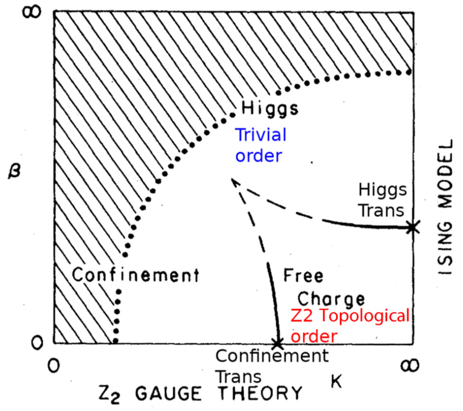
Figure 5: The phase diagram of eqn. (VII.2).

To see the $\widetilde{Z}_{2}^{(1)}$ 1-symmetry explicitly, we need to do a duality transformation to obtain a new model with a spin-1/2 living on each square face $\langle ijkl\rangle$ of the cubic lattice. Let $\widetilde{X}_{ijkl},\widetilde{Y}_{ijkl},\widetilde{Z}_{ijkl}$ be the Pauli operators acting on the spin-1/2 on face $\langle ijkl\rangle$. The duality mapping is given by

$$X_{ij}X_{jk}X_{kl}X_{li} \to\widetilde{X}_{ijkl}, Z_{ij} \to\prod_{k,l\text{ next to }i,j}\widetilde{Z}_{ijkl},$$

$$\prod_{\langle ijkl\rangle\in c}\widetilde{X}_{ijkl} =1.$$ (105)

where $\prod_{\langle ijkl\rangle\in c}$ is the product over all the six faces of a cube $c$. The dual Hamiltonian is given by

$$\widetilde{H} =-B\sum_{\langle ij\rangle}\prod_{k,l\text{ next to }i,j}\widetilde{Z}_{ijkl}-J\sum_{\langle ijkl\rangle}\widetilde{X}_{ijkl}$$

$$\ \ \ \ +\widetilde{U}\sum_{c}\left(1-\prod_{\langle ijkl\rangle\in c}\widetilde{X}_{ijkl}\right),$$ (106)

where $\widetilde{U}\to\infty$.

When $B>0$ and $J=0$, the above dual model $\widetilde{H}$ has ground state with a dual $\widetilde{Z}_{2}$ topological order (which corresponds to the confined phase with the trivial $Z_{2}$ topological order in the original model (VII.2)). When $B=0$ and $J>0$, the model has trivial product state $|\{\widetilde{X}_{ijkl}=1\}\rangle$ as its ground state and is in the dual trivial phase (which corresponds to the phase with the $Z_{2}$ topological order in the original model (VII.2)). Changing from $(B>0,J=0)$ to $(B=0,J>0)$ induces a dual confinement transition, while changing from $(B=0,J>0)$ to $(B>0,J=0)$ induces a confinement transition.

The dual model $\widetilde{H}$ explicitly has a $\widetilde{Z}_{2}^{(1)}$ 1-symmetry generated by the following membrane operator

$$C_{\widetilde{Z}_{2}^{(1)}}(M^{2})=\prod_{\langle ijkl\rangle\in M^{2}}\widetilde{X}_{ijkl}.$$ (107)

The membrane operator $C_{\widetilde{Z}_{2}^{(1)}}(M^{2})$ acts on a membrane $M^{2}$ which is formed by the squares of the lattice. Such a $\widetilde{Z}_{2}^{(1)}$ 1-symmetry is spontaneously broken in the phase with dual $\widetilde{Z}_{2}$ topological order (the confined phase with the trivial $Z_{2}$ topological order), and is unbroken in the dual trivial phase (the phase with the $Z_{2}$ topological order). If the confinement transition from the $\widetilde{Z}_{2}$ topological order to the trivial order is given by a single critical point, then such a gapless critical state will have the full $Z_{2}^{(1)}\vee\widetilde{Z}_{2}^{(1)}$ categorical symmetry which is not spontaneously broken.

It is well known that there are two ways to go from 3+1D $Z_{2}$ topological order (i.e. $Z_{2}$ gauge theory) to trivial order, either via Higgs condensation or via confinement. LABEL:FS7982 studied a model defined by the 3+1D path integral for the following action

$$S =\frac{K}{2}\sum_{\langle ijkl\rangle}\sigma_{ij}\sigma_{jk}\sigma_{kl}\sigma_{li}+\frac{\beta}{2}\sum_{ij}\phi_{i}^{\dagger}\sigma_{ij}\phi_{j}$$

$$\sigma_{ij}=\pm 1,\ \ \ \phi_{i}=\pm 1.$$ (108)

The model has $Z_{2}$ topological order when $\beta\sim 0$ and $K\sim+\infty$. The model has trivial order when $\beta\sim+\infty$ or $K\sim 0$ (see Figure 5).

When $K=+\infty$, as we change $\beta$ from 0 to $+\infty$, the model goes through a second-order Ising transition (i.e. Higgs transition) described by a critical point. When $\beta=0$, as we change $K$ from 0 to $+\infty$, the model goes through a first-order confinement transitionCreutz et al. (1979). Let us assume that we can modify the model to make the confinement transition to be a continuous transition described by a critical point. One may wonder whether the two critical points for the two transitions are the same or not.

Our above discussions suggest that the two critical points to be different since they have different categorical symmetries. One has $Z_{2}\vee Z_{2}^{(2)}$ categorical symmetry and the other has $Z_{2}^{(1)}\vee\widetilde{Z}_{2}^{(1)}$ categorical symmetry, and $Z_{1}(3{{\cal R}\text{ep}}(Z_{2}))$ are different from $Z_{1}\left(3{{\cal V}\text{ec}}_{Z_{2}^{(1)}}\right)$. Thus categorical symmetries deepen our understanding of the Higgs transition and the confinement transition, as well as their relation.

VII.3 The emergent maximal categorical symmetry

We know that the 1+1D critical point of $Z_{2}$ symmetry breaking transition has the following modular invariant partition function:

$$Z(\tau)=|\chi^{\text{Is}}_{0}(\tau)|^{2}+|\chi^{\text{Is}}_{\frac{1}{2}}(\tau)|^{2}+|\chi^{\text{Is}}_{\frac{1}{16}}(\tau)|^{2}.$$ (109)

Such a CFT and its modular invariant partition function has no gravitational anomaly and can be realized by a 1+1D lattice model. In other words, such a CFT can be realized on the boundary of a trivial 2+1D topological order. Since the 1+1D categorical symmetry is just another name for 1+1D non-invertible gravitational anomaly, which is another name for 2+1D topological order, we say the above formulation of the $Z_{2}$-symmetry-breaking critical point does not expose any categorical symmetry.

We know that the critical point actually has a $Z_{2}$ symmetry. To expose the $Z_{2}$ symmetry, we consider systems with $Z_{2}$-symmetry twisted boundary condition, as well as even-odd $Z_{2}$ charges. This gives us a 4-component partition function as in eqn. (39). The modular covariance of the 4-component partition function implies that the CFT have a non-invertible gravitational anomaly, which is characterized by the 2+1D $Z_{2}$ gauge theory. In other words, the CFT (39) has the $Z_{2}\vee\widetilde{Z}_{2}$ categorical symmetry.

We see that the different formulation of the $Z_{2}$-symmetry-breaking critical point reveal or expose different emergent symmetries. The first modular invariant formulation (109) does not reveal any categorical symmetry. The second formulation (39) exposes the $Z_{2}\vee\widetilde{Z}_{2}$ categorical symmetry. In particular, it exposes both the $Z_{2}$ symmetry and the $\widetilde{Z}_{2}$ dual symmetry.

Here, we would like to ask whether the $Z_{2}$-symmetry-breaking critical point has additional emergent symmetries. What is the maximal categorical symmetry of the $Z_{2}$-symmetry-breaking critical point? In fact, the $Z_{2}\vee\widetilde{Z}_{2}$ categorical symmetry is not maximal. The $Z_{2}$-symmetry-breaking critical point has even larger categorical symmetry.

One way to find large emergent categorical symmetry of a CFT, is to choose a smaller set of conformal characters as the trivial component of the partition function. For the example of the $Z_{2}$-symmetry-breaking critical point, we may choose the trivial component of the partition function to be

$$Z_{\mathbf{1}}(\tau)=|\chi^{\text{Is}}_{0}(\tau)|^{2}.$$ (110)

Such a partition function is a part of a 9-component modular covariant partition function

$$Z_{h,h^{\prime}}=\chi^{\text{Is}}_{h}(\tau)\bar{\chi}^{\text{Is}}_{h^{\prime}}(\bar{\tau}),\ \ \ h,h^{\prime}=0,\frac{1}{2},\frac{1}{16},$$ (111)

where $Z_{\mathbf{1}}(\tau)=|\chi^{\text{Is}}_{0}(\tau)|^{2}=Z_{0,0}(\tau)$. The modular covariance of the 9-component partition function implies that the CFT have a non-invertible gravitational anomaly, which is characterized by 2+1D double-Ising $3^{B}_{1/2}\boxtimes 3^{B}_{-1/2}$ topological order (using the notation in LABEL:W150605768 where $n^{B}_{c}$ represents a bosonic topological other with $n$ superselection sectors and chiral central charge $c$, and $\boxtimes$ is the stacking operation). In other words, the CFT (111) has a double-Ising $3^{B}_{1/2}\boxtimes 3^{B}_{-1/2}$ categorical symmetry. In particular, eqn. (111) exposes both the $Z_{2}$ symmetry and the $\widetilde{Z}_{2}$ dual symmetry, as well as the $Z_{2}$ symmetry from the Kramers-Wannier duality. We believe that the double-Ising categorical symmetry $3^{B}_{1/2}\boxtimes 3^{B}_{-1/2}$ is the maximal emergent categorical symmetry of the $Z_{2}$-symmetry-breaking critical point.Moore and Seiberg (1989)

There is another way to obtain the larger emergent categorical symmetry. We know that the 1+1D $Z_{2}$-symmetry-breaking critical point can be viewed as a boundary of 2+1D $Z_{2}$ topological order, which has four types of topological excitations $\mathbf{1},e,m,f$. This point of view reveals the emergent $Z_{2}\vee\widetilde{Z}_{2}$ categorical symmetry of the critical point. We can fine-tune the 2+1D $Z_{2}$ topological order to make it to have a $e,m$ exchange symmetry. We can then gauge such a $e,m$ exchange symmetry.Barkeshli et al. (2019); Heinrich et al. (2016) The resulting 2+1D topological order is the double-Ising topological order $3^{B}_{1/2}\boxtimes 3^{B}_{-1/2}$. This corresponds to the large double-Ising $3^{B}_{1/2}\boxtimes 3^{B}_{-1/2}$ categorical symmetry.

Next, let us consider another example of $c=\bar{c}=\frac{7}{10}$ CFT. The 4-component partition function (45) reveal the emergent $Z_{2}\vee\widetilde{Z}_{2}$ categorical symmetry of the CFT. However, the $c=\bar{c}=\frac{7}{10}$ CFT has a larger emergent categorical symmetry, as exposed by the following 36-component partition function

$$\begin{split}Z_{h,h^{\prime}}=&\chi^{5,4}_{h}(\tau)\bar{\chi}^{5,4}_{h^{\prime}}(\bar{\tau}),\\ h,h^{\prime}=&\,0,\frac{3}{2},\frac{7}{16},\frac{1}{10},\frac{3}{5},\frac{3}{80}.\end{split}$$ (112)

Such a maximal emergent categorical symmetry is characterized by the 2+1D topological order $6^{B}_{7/10}\boxtimes 6^{B}_{-7/10}$ (again using the notation in LABEL:W150605768). In fact, $6^{B}_{-7/10}=2^{B}_{14/5}\boxtimes 3^{B}_{-7/2}$, where $2^{B}_{14/5}$ is the Fibonacci topological order, and $3^{B}_{-7/2}$ is a twisted Ising topological order, whose $\sigma$ anyon has a topological spin $e^{-\hskip 1.0pt\mathrm{i}\hskip 1.0pt2\pi\frac{7}{16}}$.

The above two examples suggest that a CFT can have a maximal categorical symmetry. We hope that the maximal categorical symmetry carries a lot of information about the corresponding CFT. It may be possible that we can use the maximal categorical symmetry to characterize or even classify the CFTs. Thus maximal categorical symmetry represents a research direction that may allow us to develop a systematic theory of gapless CFTs, via mapping class group representations for various spacetime topologies. We also note that the maximal categorical symmetry of a 1+1D CFT has a form ${\cal C}\boxtimes\bar{\cal C}$, where ${\cal C}$ is a 2+1D topological order and $\bar{\cal C}$ is the time-reversal conjugate of ${\cal C}$. This structure was referred to as naturality principle of maximally extended CFT in LABEL:MS8916. In fact, modular tensor category – the mathematical description of bosonic topological orders, has been used to classify all rational modular invariant conformal field theories Fuchs et al. (2002, 2002, 2004a, 2004b, 2005); Fjelstad et al. (2006); Runkel et al. (2007); Kong and Runkel (2009); Kong (2011); Kong et al. (2013) Such classification has also been interpretated physically in terms of surface operators of $2+1$D topological order Kapustin and Saulina (2010).

VIII Summary

Figure 6: (a) A CFT with 0-symmetry $G$ is described by a AdS/CFT dual that contains a $G$ gauge theory in the AdS space in one higher dimension. (b) The CFT at the transition of spontaneously $G$-symmetry breaking has a categorical symmetry $\mathcal{G}^{n}_{G}=G\vee G^{(n-1)}$ described by excitations in a $G$-gauge theory in one higher dimension.

Figure 7: A combination of the holographic picture for AdS/CFT duality and the holographic picture for emergent categorical symmetry in the CFT for the $G$-symmetry breaking transition.

In this paper, we show that a quantum system in $n$-dimensional space with a 0-symmetry $G$ actually has a larger symmetry, which includes both the 0-symmetry $G$ and an algebraic $(n-1)$-symmetry, denoted as $G^{(n-1)}$, whose transformations are given by Wilson loop operators. In fact, the $G$-symmetric quantum system actually has a larger categorical symmetry characterized by a braided fusion $n$-category $\mathcal{G}^{n}_{G}$. We also denote the categorical symmetry $\mathcal{G}^{n}_{G}$ as $G\vee G^{(n-1)}$, since it includes both the 0-symmetry $G$ and the algebraic $(n-1)$-symmetry $G^{(n-1)}$.

We find that any gapped state in a system with a categorical symmetry must partially (and only partially) break the categorical symmetry spontaneously. However, for the gapless critical state at the transition of the spontaneous $G$-symmetry breaking, the categorical symmetry $G\vee G^{(n-1)}$ is not broken. In particular, the critical state has both the 0-symmetry $G$ and the algebraic $(n-1)$-symmetry $G^{(n-1)}$.

It was proposed that a CFT in $n$-dimensional space with 0-symmetry $G$ has a AdS/CFT dual that contain a $G$-gauge theory in the $(n+1)$d AdS space (see Fig. 6a).Maldacena (1998); Witten (1998); Klebanov and Witten (1999); Harlow and Ooguri (2018) If the AdS/CFT dual contains only a $G$-gauge theory (with the fluctuations of both gauge charges and gauge flux) and gravity in the $(n+1)$d AdS space (see Fig. 6a), then the corresponding CFT in $n$-dimensional space must be a particular one with 0-symmetry $G$. But there are many CFT’s with 0-symmetry $G$. Which is the right one? The result in this paper (see Fig. 6b) suggests that: It is the CFT at the transition of the spontaneous $G$-symmetry breaking that is dual to a theory that contains only a $G$-gauge theory and gravity in the $(n+1)$d AdS space. This is because the specific CFT has the categorical symmetry $G\vee G^{(n-1)}$, whose excitations matches that of the dual theory in the AdS bulk. In other words, the whole Fig. 6a corresponds to the CFT boundary in Fig. 6b. This is demonstrated in Fig. 7. The categorical symmetry of a CFT can help us to select the AdS/CFT dual of the CFT, which is an important application of the categorical symmetry.

We would like to mention that the close relation between topological order and its canonical gapless CFT boundary has been discussed extensively in LABEL:KZ170501087,KZ190504924,KZ191201760, for the case of 2+1D topological order and 1+1D gapless boundary. A notion of topological Wick-rotation is introduced to describe how a 2+1D topological order can determine a canonical 1+1D CFT boundary.

We would like to thank Liang Kong, Tian Lan, Shu-heng Shao, Hao Zheng for many helpful discussions. This research was partially supported by NSF DMS-1664412. This work was also partially supported by the Simons Collaboration on Ultra-Quantum Matter, which is a grant from the Simons Foundation (651440).

Appendix A List of terminologies

Here, we explain some mathematical terminologies used in this paper, at the level of physical rigorousness. An ordinary category has objects and morphisms (also called 1-morphisms), and it is also called 1-category. A 2-category generalizes this by also including 2-morphisms between the 1-morphisms. Continuing this up to $n$-morphisms between $(n-1)$-morphisms gives an $n$-category.

In condensed matter physics, a $n$-category can correspond to a collection of topological orders in $n$D spacetime. The topological orders in the collection correspond to the simple objects in the category. The composite objects correspond to degenerate states where several different topological orders happen to have the same energy. The gapped domain walls between different topological orders correspond to 1-morphisms between different simple objects. The gapped domain walls within the same topological order correspond to 1-morphisms between the same simple object. The domain walls (1-morphisms) can also have domain walls with one lower dimension between them, which correspond to 2-morphisms, etc . In general, a $m$-morphism that connects the trivial $m-1$ morphism to itself corresponds to a codimension-$m$ excitation. A $m$-morphism that connects a non-trivial $m-1$ morphism to itself corresponds to a domain wall on the codimension-$m-1$ excitation. A $m$-morphism that connects two $m-1$ morphisms corresponds to a domain wall between the two codimension-$m-1$ excitations. A $n$-morphism corresponds to an “instanton” in spacetime (i.e. an insertion of a local operator in spacetime). A $(n-1)$-morphism corresponds a point-like excitation.

Two topological orders can be stacked to form the third topological order. Under the stacking operation, topological orders form a monoid (which is similar to a group, but no need for an inverse operation) Kong and Wen (2014). If we include the stacking operation in the $n$-category, the $n$-category will become a fusion $n$-category. Thus a collection of topological orders in $n$-dimensional spacetime is actually described by a monoidal $n$-category.

The excitations in a single topological order in $n$D spacetime is described by a fusion $(n-1)$-category. Now the objects in the fusion $(n-1)$-category correspond codimension-1 excitations (domain walls). The 1-morphisms correspond codimension-2 excitations (domain walls on domain walls), etc .

An example of fusion 1-category is ${{\cal V}\text{ec}}$. The objects in ${{\cal V}\text{ec}}$ are the vector spaces. The simple objects are the (equivalent classes of) 1-dimensional vector spaces and composite objects are multi-dimensional vector spaces. There is only one simple object. We see that composite objects are direct sums of simple objects. The morphisms (the 1-morphisms) correspond to the linear operators acting on the vector spaces. The tensor product of the vector spaces defines the fusion of the objects. We see that 1-dimensional vector space is the unit of the tensor product, and hence the simple object is the unit of the fusion. We also call such a fusion unit as the trivial object. The 1-morphisms that connect the simple object to itself is proportional to the one-by-one identity operator, and thus are also trivial. So we refer fusion 1-category ${{\cal V}\text{ec}}$ as trivial category. We also have trivial higher category, which has only one simple non-descendant morphism (which are not condensation of other excitationsGaiotto and Johnson-Freyd (2019); Johnson-Freyd (2020); Kong et al. (2020a, b)) at every level. We denote the trivial higher category as $n{{\cal V}\text{ec}}$.

Another example of fusion $n$-category is ${{\cal R}\text{ep}}(G)$. The $(n-1)$-morphisms in ${{\cal R}\text{ep}}(G)$ are the representations of the group $G$ which correspond to point-like excitations in $n$-dimensional space. The tensor product of the $G$-representations defines the fusion of the $(n-1)$-morphisms. The simple $(n-1)$-morphisms are the (equivalent classes of) irreducible representations and composite objects are the reducible representations. The reducible representations are direct sums of irreducible representations, and thus composite morphisms are direct sums of simple morphisms. The $n$-morphisms correspond the symmetric operators acting one on group representations.

All the 1-morphisms, 2-morphisms on the trivial object in a fusion $n$-category form a braided fusion $(n-1)$-category. It can be used to describe codimension-2 and higher excitations in an anomaly-free topological order (after dropping the codimension-1 excitations which are always descendent for anomaly-free topological orders).

We also need a notion of local fusion $n$-category: A fusion $n$-category ${\cal F}$ is local if we can add morphisms in a consistent way, such that all the resulting simple morphisms are isomorphic to the trivial one. Physically, the process of “adding morphisms” corresponds to explicit breaking of the (algebraic higher) symmetry. This is because, ${\cal F}$ only has morphisms that correspond to symmetric operators. Adding morphisms means include morphisms that correspond to symmetry breaking operators. If after breaking all the symmetry, ${\cal F}$ becomes a trivial product phase of bosons or fermions, then ${\cal F}$ is a local fusion $n$-category.

Appendix B Proof of equivalence of the 1d (projected) $Z_{2}$ minimally coupled model and the (projected) Ising model

We are going to prove that the (projected) minimally coupled model eqn. (II.3), the (projected) Ising model eqn. (10) and the (projected) dual Ising model eqn. (11) are all equivalent. In this subsection, we always consider the projected sub-Hilbert space respectively.

The strategy is to show that in the minimally coupled model, the Hamiltonian is built from the logical operators within a stabilized subspace. We begin with $2N$ physical qubits on $2N$ sites. We take those states stabilized by $Z_{2i-1}Z_{2i}Z_{2i+1}$, for $i=1,\cdots,N$. This is to constraint ourselves to states $Z_{2i-1}Z_{2i}Z_{2i+1}=1$.

We first show that the minimally coupled model is equivalent to the Ising model. The proof uses the stabilized code formalism in quantum information (QI).

For simplicity, we switch the notation in the minimal coupled model to that in QI, $X_{i}\rightarrow X_{2i-1},\widetilde{X}_{i+\frac{1}{2}}\rightarrow X_{2i}$, and similarly for the Pauli $Z$’s. In this way, the low energy constraints in the limit $U\rightarrow\infty$ are mapped to the stabilizers. And the Hamiltonian becomes

$$H=-B\sum_{i}X_{2i}X_{2i+1}X_{2i+2}-J\sum_{i}Z_{2i},$$ (113)

acting on the $2N$ number of physical qubits. And there are then in total $2^{N}$ logical qubits.

First, we show

$$\mathcal{X}_{i}=X_{2i}X_{2i+1}X_{2i+2},~{}~{}~{}\mathcal{Z}_{i}=Z_{2i+1},$$ (114)

are the Pauli-$X$ and Pauli-$Z$ operators on the logical qubits. (And $\mathcal{X}_{N}=X_{2N}X_{1}X_{2},\mathcal{Z}_{N}=Z_{1}$.) Obviously, they satisfy the algebra of the Pauli matrices, and each of them commute with the stabilizers. Since there are $N$ Pauli-$Z$ operators we find, their eigenvalues labels are in one-to-one correspond to the states in the stabilized space. Therefore, these logical Pauli operators $\{\mathcal{X}_{i},\mathcal{Z}_{i}|i=1,\cdots,N\}$ form a complete basis for all operators acting on the logic qubits.

Then we find that $\mathcal{Z}_{i}\mathcal{Z}_{i+1}=Z_{2i+2}$ (and $\mathcal{Z}_{N}\mathcal{Z}_{1}=Z_{2}$) are the same as a pair of Pauli-$Z$ operators on the logical qubits. It follows from (114) that $\mathcal{Z}_{i}\mathcal{Z}_{i+1}=Z_{2i+1}Z_{2i+3}(Z_{2i+1}Z_{2i+2}Z_{2i+3})$, where it is a stabilizer that we multiply on in the bracket. The model in terms of logical operators becomes

$$H=-B\sum_{i}\mathcal{X}_{i}-J\sum_{i}\mathcal{Z}_{i-1}\mathcal{Z}_{i}.$$ (115)

Finally, the global symmetry operator $\prod_{i}X_{2i+1}$ in the minimally coupled model also maps to $\prod_{i}\mathcal{X}_{i}$, the global $Z_{2}$ symmetry operator on the logical qubits. We may, of course, add this operator initially to the set of stabilizers and the analysis remains the same but with $2^{N-1}$ logical qubits.

There is a caveat in this proof. If different models can be mapped to the same Hamiltonian on the same set of logical qubits defined in a stabilized space, they are indeed the same at the algebraic level. However, we need to further check if they have the same “locality property”. Even though it is hard to define the property generically, for the one-dimensional models we study here, they all have the properties that neighboring logical Pauli operators come from neighboring local terms composed of physical Pauli operators.

Appendix C Non-on-site $Z_{2}$ symmetry transformations

The non-on-site $Z_{2}$ symmetry transformation $U=\prod_{i}X_{i}\prod_{i}s_{i-\frac{1}{2},i+\frac{1}{2}}$ (where $s_{ij}$ is given in eqn. (IV.1)) transforms $X_{i}$ in the following way:

$$\ \ \ \ \left(\prod_{j}X_{j}\prod_{j}s_{j,j+1}\right)X_{i}\left(\prod_{j}X_{j}\prod_{j}s_{j,j+1}\right)$$

$$=\frac{1-Z_{i-1}+Z_{i}+Z_{i-1}Z_{i}}{2}\frac{1-Z_{i}+Z_{i+1}+Z_{i}Z_{i+1}}{2}X_{i}$$

$$\ \ \ \ \frac{1-Z_{i-1}+Z_{i}+Z_{i-1}Z_{i}}{2}\frac{1-Z_{i}+Z_{i+1}+Z_{i}Z_{i+1}}{2}$$

$$=\frac{1-Z_{i-1}+Z_{i}+Z_{i-1}Z_{i}}{2}\frac{1-Z_{i}+Z_{i+1}+Z_{i}Z_{i+1}}{2}$$

$$\ \ \ \ \frac{1-Z_{i-1}-Z_{i}-Z_{i-1}Z_{i}}{2}\frac{1+Z_{i}+Z_{i+1}-Z_{i}Z_{i+1}}{2}X_{i}$$

$$=\Big{(}\frac{1-Z_{i-1}+Z_{i}+Z_{i-1}Z_{i}}{2}\frac{1-Z_{i-1}-Z_{i}-Z_{i-1}Z_{i}}{2}\Big{)}$$

$$\ \ \ \ \Big{(}\frac{1-Z_{i}+Z_{i+1}+Z_{i}Z_{i+1}}{2}\frac{1+Z_{i}+Z_{i+1}-Z_{i}Z_{i+1}}{2}\Big{)}X_{i}$$

$$=\frac{(1-Z_{i-1})-(1+Z_{i-1})}{2}\frac{(1+Z_{i+1})-(1-Z_{i+1})}{2}X_{i}$$

$$=-Z_{i-1}X_{i}Z_{i+1}.$$ (116)

In other words

$$X_{i}\leftrightarrow-Z_{i-1}X_{i}Z_{i+1}.$$ (117)

References

- Landau (1937a) L. D. Landau, Phys. Z. Sowjetunion 11, 26 (1937a).
- Landau (1937b) L. D. Landau, Phys. Z. Sowjetunion 11, 545 (1937b).
- Ginsparg (1991) P. Ginsparg, (1991), hep-th/9108028 .
- Di Francesco et al. (1997) P. Di Francesco, P. Mathieu, and D. S??n??chal, Conformal Field Theory (Springer New York, 1997).
- Lan et al. (2018) T. Lan, L. Kong, and X.-G. Wen, Phys. Rev. X 8, 021074 (2018), arXiv:1704.04221 .
- Lan and Wen (2019) T. Lan and X.-G. Wen, Phys. Rev. X 9, 021005 (2019), arXiv:1801.08530 .
- Kong et al. (2020a) L. Kong, T. Lan, X.-G. Wen, Z.-H. Zhang, and H. Zheng, J. High Energ. Phys. 2020, 93 (2020a), arXiv:2003.08898 .
- Kong et al. (2020b) L. Kong, T. Lan, X.-G. Wen, Z.-H. Zhang, and H. Zheng, (2020b), arXiv:2005.14178 .
- Gaiotto et al. (2015) D. Gaiotto, A. Kapustin, N. Seiberg, and B. Willett, J. High Energ. Phys. 2015, 172 (2015), arXiv:1412.5148 .
- Fröhlich et al. (2007) J. Fröhlich, J. Fuchs, I. Runkel, and C. Schweigert, Nucl. Phys. B 763, 354 (2007), arXiv:hep-th/0607247 .
- Davydov et al. (2011) A. Davydov, L. Kong, and I. Runkel, Adv. Theor. Math. Phys. 15, 43 (2011), arXiv:1004.4725 .
- Chang et al. (2019) C.-M. Chang, Y.-H. Lin, S.-H. Shao, Y. Wang, and X. Yin, J. High Energ. Phys. 2019, 26 (2019), arXiv:1802.04445 .
- Thorngren and Wang (2019) R. Thorngren and Y. Wang, (2019), arXiv:1912.02817 .
- Kong et al. (2019) L. Kong, W. Yuan, and H. Zheng, (2019), arXiv:1912.13168 .
- Kapustin and Thorngren (2013) A. Kapustin and R. Thorngren, (2013), arXiv:1309.4721 .
- Thorngren and von Keyserlingk (2015) R. Thorngren and C. von Keyserlingk, (2015), arXiv:1511.02929 .
- Ibieta-Jimenez et al. (2020) J. Ibieta-Jimenez, M. Petrucci, L. Q. Xavier, and P. Teotonio-Sobrinho, J. High Energ. Phys. 2020 (2020), 10.1007/jhep03(2020)167, arXiv:1711.04186 .
- Kobayashi et al. (2019) R. Kobayashi, K. Shiozaki, Y. Kikuchi, and S. Ryu, Phys. Rev. B 99, 014402 (2019), arXiv:1805.05367 .
- Lake (2018) E. Lake, (2018), arXiv:1802.07747 .
- Wen (2019) X.-G. Wen, Phys. Rev. B 99, 205139 (2019), arXiv:1812.02517 .
- Wan and Wang (2019) Z. Wan and J. Wang, Phys. Rev. D 99, 065013 (2019), arXiv:1812.11955 .
- Wan and Wang (2019) Z. Wan and J. Wang, Annals of Mathematical Sciences and Applications 4, 107 (2019), arXiv:1812.11967 .
- Kitaev (2003) A. Kitaev, Ann. Phys. 303, 2 (2003).
- Wen (2003) X.-G. Wen, Phys. Rev. Lett. 90, 016803 (2003), arXiv:quant-ph/0205004 .
- Levin and Wen (2003) M. Levin and X.-G. Wen, Phys. Rev. B 67, 245316 (2003), arXiv:cond-mat/0302460 .
- Nussinov and Ortiz (2009a) Z. Nussinov and G. Ortiz, Proceedings of the National Academy of Sciences 106, 16944 (2009a), arXiv:cond-mat/0605316 .
- Nussinov and Ortiz (2009b) Z. Nussinov and G. Ortiz, Ann. Phys. 324, 977 (2009b), arXiv:cond-mat/0702377 .
- Yoshida (2011) B. Yoshida, Ann. Phys. 326, 15 (2011), arXiv:1007.4601 .
- Bombín (2014) H. Bombín, Commun. Math. Phys. 327, 387 (2014), arXiv:1107.2707 .
- Kong and Wen (2014) L. Kong and X.-G. Wen, (2014), arXiv:1405.5858 .
- Ji and Wen (2019) W. Ji and X.-G. Wen, Phys. Rev. Research 1, 033054 (2019), arXiv:1905.13279 .
- Maldacena (1998) J. Maldacena, Adv. Theor. Math. Phys. 2, 231 (1998), hep-th/9711200 .
- Witten (1998) E. Witten, Advances in Theoretical and Mathematical Physics 2, 253 (1998), arXiv:hep-th/9802150 .
- Klebanov and Witten (1999) I. R. Klebanov and E. Witten, Nuclear Physics B 556, 89 (1999), arXiv:hep-th/9905104 .
- Harlow and Ooguri (2018) D. Harlow and H. Ooguri, (2018), arXiv:1810.05338 .
- Belavin et al. (1984) A. Belavin, A. Polyakov, and A. Zamolodchikov, Nucl. Phys. B 241, 333 (1984).
- Zamolodchikov and Fateev (1985) A. Zamolodchikov and V. Fateev, Sov. Phys. JETP 62, 215 (1985).
- Verresen et al. (2019) R. Verresen, R. Thorngren, N. G. Jones, and F. Pollmann, (2019), arXiv:1905.06969 .
- Ji et al. (2020) W. Ji, S.-H. Shao, and X.-G. Wen, Phys. Rev. Research 2, 033317 (2020), arXiv:1909.01425 .
- Levin (2020) M. Levin, Commun. Math. Phys. 378, 1081 (2020), arXiv:1903.09028 .
- Harlow and Ooguri (2019) D. Harlow and H. Ooguri, Phys. Rev. Lett. 122, 191601 (2019), arXiv:1810.05337 [hep-th] .
- Doplicher (1982) S. Doplicher, Commun. Math. Phys. 85, 73 (1982).
- Doplicher and Longo (1983) S. Doplicher and R. Longo, Commun. Math. Phys. 88, 399 (1983).
- Buchholz et al. (1986) D. Buchholz, S. Doplicher, and R. Longo, Annals Phys. 170, 1 (1986).
- Verstraete and Cirac (2004) F. Verstraete and J. Cirac, (2004), cond-mat/0407066 .
- Vidal (2007) G. Vidal, Phys. Rev. Lett. 99, 220405 (2007), arXiv:cond-mat/0512165 .
- Levin and Nave (2007) M. Levin and C. P. Nave, Phys. Rev. Lett. 99, 120601 (2007).
- Gu and Wen (2009) Z.-C. Gu and X.-G. Wen, Phys. Rev. B 80, 155131 (2009), arXiv:0903.1069 .
- Chen et al. (2012) X. Chen, Z.-C. Gu, Z.-X. Liu, and X.-G. Wen, Science 338, 1604 (2012), arXiv:1301.0861 .
- Chen et al. (2020) W.-Q. Chen, C.-M. Jian, L. Kong, Y.-Z. You, and H. Zheng, Phys. Rev. B 102, 045139 (2020), arXiv:1903.12334 .
- Kong and Zheng (2018) L. Kong and H. Zheng, Nucl. Phys. B 927, 140 (2018), arXiv:1705.01087 .
- Kong and Zheng (2020) L. Kong and H. Zheng, J. High Energ. Phys. 2020, 150 (2020), arXiv:1905.04924 .
- Kong and Zheng (2019) L. Kong and H. Zheng, (2019), arXiv:1912.01760 .
- Dijkgraaf and Witten (1990) R. Dijkgraaf and E. Witten, Commun.Math. Phys. 129, 393 (1990).
- ’t Hooft (1980) G. ’t Hooft, NATO Adv. Study Inst. Ser. B Phys. 59, 135 (1980).
- Wen (2013) X.-G. Wen, Phys. Rev. D 88, 045013 (2013), arXiv:1303.1803 .
- Freedman et al. (2004) M. Freedman, C. Nayak, K. Shtengel, K. Walker, and Z. Wang, Ann. Phys. 310, 428 (2004), arXiv:cond-mat/0307511 .
- Levin and Wen (2005) M. A. Levin and X.-G. Wen, Phys. Rev. B 71, 045110 (2005), arXiv:cond-mat/0404617 .
- Chen et al. (2011) X. Chen, Z.-X. Liu, and X.-G. Wen, Phys. Rev. B 84, 235141 (2011), arXiv:1106.4752 .
- Gukov and Kapustin (2013) S. Gukov and A. Kapustin, (2013), arXiv:1307.4793 [hep-th] .
- Gaiotto and Johnson-Freyd (2019) D. Gaiotto and T. Johnson-Freyd, J. High Energ. Phys. 2019, 7 (2019), arXiv:1905.09566 .
- Johnson-Freyd (2020) T. Johnson-Freyd, (2020), arXiv:2003.06663 .
- Lan et al. (2017) T. Lan, L. Kong, and X.-G. Wen, Phys. Rev. B 95, 235140 (2017), arXiv:1602.05946 .
- Freed and Teleman (2018) D. S. Freed and C. Teleman, (2018), arXiv:1806.00008 [math.AT] .
- Kong et al. (2015) L. Kong, X.-G. Wen, and H. Zheng, (2015), arXiv:1502.01690 .
- Kong et al. (2017) L. Kong, X.-G. Wen, and H. Zheng, Nucl. Phys. B 922, 62 (2017), arXiv:1702.00673 .
- Read and Sachdev (1991) N. Read and S. Sachdev, Phys. Rev. Lett. 66, 1773 (1991).
- Wen (1991) X.-G. Wen, Phys. Rev. B 44, 2664 (1991).
- Gattringer (2014) C. Gattringer, PoS LATTICE2013, 002 (2014), arXiv:1401.7788 [hep-lat] .
- Baez and Schreiber (2007) J. C. Baez and U. Schreiber, Contemp. Math. 431, AMS, Providence, Rhode Island , 7 (2007), math/0511710 .
- Girelli et al. (2008) F. Girelli, H. Pfeiffer, and E. M. Popescu, J. Math. Phys. 49, 032503 (2008), arXiv:0708.3051 .
- Baez and Huerta (2010) J. C. Baez and J. Huerta, Gen Relativ Gravit 43, 2335 (2010), arXiv:1003.4485 .
- Bullivant et al. (2017a) A. Bullivant, M. Calcada, Z. Kádár, P. Martin, and J. a. F. Martins, Phys. Rev. B 95, 155118 (2017a), arXiv:1606.06639 .
- Bullivant et al. (2017b) A. Bullivant, M. Calcada, Z. Kádár, P. Martin, and J. F. Martins, Reviews in Mathematical Physics (2017b), 10.1142/S0129055X20500117, arXiv:1702.00868 .
- Zhu et al. (2019) C. Zhu, T. Lan, and X.-G. Wen, Phys. Rev. B 100, 045105 (2019), arXiv:1808.09394 .
- Fradkin and Shenker (1979) E. Fradkin and S. H. Shenker, Phys. Rev. D 19, 3682 (1979).
- Creutz et al. (1979) M. Creutz, L. Jacobs, and C. Rebbi, Phys. Rev. D 20, 1915 (1979).
- Wen (2015) X.-G. Wen, Nat. Sci. Rev. 3, 68 (2015), arXiv:1506.05768 .
- Moore and Seiberg (1989) G. Moore and N. Seiberg, Nuclear Physics B 313, 16 (1989).
- Barkeshli et al. (2019) M. Barkeshli, P. Bonderson, M. Cheng, and Z. Wang, Phys. Rev. B 100, 115147 (2019).
- Heinrich et al. (2016) C. Heinrich, F. Burnell, L. Fidkowski, and M. Levin, Phys. Rev. B 94, 235136 (2016), arXiv:1606.07816 .
- Fuchs et al. (2002) J. Fuchs, I. Runkel, and C. Schweigert, Nucl. Phys. B 624, 452 (2002), arXiv:hep-th/0110133 .
- Fuchs et al. (2002) J. Fuchs, I. Runkel, and C. Schweigert, Nuclear Physics B 646, 353 (2002), arXiv:hep-th/0204148 .
- Fuchs et al. (2004a) J. Fuchs, I. Runkel, and C. Schweigert, Nuclear Physics B 678, 511 (2004a), arXiv:hep-th/0306164 .
- Fuchs et al. (2004b) J. Fuchs, I. Runkel, and C. Schweigert, Nuclear Physics B 694, 277 (2004b), arXiv:hep-th/0403157 .
- Fuchs et al. (2005) J. Fuchs, I. Runkel, and C. Schweigert, Nuclear Physics B 715, 539 (2005), arXiv:hep-th/0412290 .
- Fjelstad et al. (2006) J. Fjelstad, J. Fuchs, I. Runkel, and C. Schweigert, Theor. Appl. Categor. 16, 342 (2006), arXiv:hep-th/0503194 .
- Runkel et al. (2007) I. Runkel, J. Fjelstad, J. Fuchs, and C. Schweigert, Contemp. Math. 431, 225 (2007), arXiv:math/0512076 .
- Kong and Runkel (2009) L. Kong and I. Runkel, Commun. Math. Phys. 292, 871 (2009), arXiv:0807.3356 .
- Kong (2011) L. Kong, (2011), arXiv:1107.3649 .
- Kong et al. (2013) L. Kong, Q. Li, and I. Runkel, (2013), arXiv:1310.1875 .
- Kapustin and Saulina (2010) A. Kapustin and N. Saulina, (2010), arXiv:1012.0911 .