Describing Migdal effects in diamond crystal with atom-centered
localized Wannier functions

Abstract

Recent studies have theoretically investigated the atomic excitation and ionization induced by the dark matter (DM)-nucleus scattering, and it is found that the suddenly recoiled atom is much more likely to excite or lose its electrons than expected. Such phenomenon is called the “Migdal effect”. In this paper, we extend the established strategy to describe the Migdal effect in isolated atoms to the case in semiconductors under the framework of tight-binding (TB) approximation. Since the localized aspects of electrons are respected in form of the Wannier functions (WFs), the extension of the existing Migdal approach for isolated atoms is much more natural, while the extensive nature of electrons in solids is reflected in the hopping integrals. We take diamond target as a concrete proof of principle for the methodology, and calculate relevant energy spectra and projected sensitivity of such diamond detector. It turns out that our method as a preliminary attempt is theoretically self-consistent and practically effective.

1 Introduction

The identity of the dark matter (DM) is one of the most puzzling problems in modern physics. Although there has been overwhelming evidence for its existence from astrophysics and cosmology, its nature still remains a mystery from a particle physical perspective. In decades, tremendous efforts are invested into the search for the weakly interacting massive particles (WIMPs), which not only take root in mere theoretical motivations, but also naturally explain the observed relic abundance in the context of thermal freeze-out. Owing to the spectacular improvements in sensitivity over recent years, the frontier of the detection has been pushed to the DM mass range around the sub-GeV scale, where traditional experiments (e.g., XENON1T Aprile:2018dbl ; Aprile:2019xxb , LUX Akerib:2018hck , PandaX Ren:2018gyx , etc. Agnese:2017jvy ; Liu:2019kzq ; Abdelhameed:2019hmk ; Agnes:2018ves ; Armengaud:2019kfj ) are expected to turn insensitive. This has motivated alternative proposals based on new detection channels and targets, such as with semiconductors Essig:2011nj ; Graham:2012su ; Essig:2015cda ; Hochberg:2016sqx , superconductors Hochberg:2015pha ; Hochberg:2016ajh , Dirac materials Hochberg:2017wce ; Coskuner:2019odd ; Geilhufe:2019ndy , superfluid helium Knapen:2016cue ; Caputo:2019cyg ; Caputo:2019xum , and through phonon excitations Knapen:2017ekk ; Griffin:2018bjn ; Campbell-Deem:2019hdx , as well as other proposals and analyses Essig:2012yx ; Lee:2015qva ; Hochberg:2015fth ; Bloch:2016sjj ; Derenzo:2016fse ; Hochberg:2016ntt ; Essig:2016crl ; Kadribasic:2017obi ; Essig:2017kqs ; Arvanitaki:2017nhi ; Budnik:2017sbu ; SHARMA2017326 ; Cavoto:2017otc ; Liang:2018bdb ; Heikinheimo:2019lwg ; Trickle:2019nya ; Trickle:2019ovy ; Catena:2019gfa .

However, a recent research Ibe2018 clarified that the sensitivity of these conventional strategies have been significantly underestimated. In contrast to the previous impression that electrons are so tightly bound to the atom that the sudden boost of a recoiled atom cannot “shake off” the outer electrons, the authors of Ref. Ibe2018 pointed out that in realistic case it takes some time for the electrons to catch up with the struck atom, and excitation and ionization are found to be more frequent than anticipated. Such phenomenon is termed “Migdal effect” in the DM literature Bernabei:2007jz ; Dolan:2017xbu ; Ibe2018 ; Bell:2019egg ; Baxter:2019pnz ; Emken:2019tni ; Essig:2019xkx .

The purpose of this study is to extend the formalism developed for isolated atoms in Ref. Ibe2018 to the case of semiconductors. Unlike the electrons exclusively bound to an individual atom, the delocalized electrons in solids are free to hop between neighboring ions, which makes a direct application of the method developed in Ref. Ibe2018 to the crystalline environment rather dubious. On the one hand, if one follows the rest frame of the suddenly recoiled nucleus in solids, the rest of the nuclei in solids will no longer be stationary either. On the other hand, if one follows the whole recoiled crystal, the highly local impulsive effect caused by the incident DM particle cannot be appropriately accounted for. To pursue a reasonable extension, we resort to the tight-binding (TB) approximation in which both the local and extensive characteristics of the Migdal effect in crystal are taken into consideration simultaneously. To be specific, we first re-express the Bloch wavefunctions in terms of the Wannier functions (WFs) that reflect the localized aspects of the itinerant electrons, and then we impose the Galilean transformation operator exclusively onto those WFs associated with the struck atom, and as a consequence the extensive aspects of electrons are effectively encoded in the hopping integrals. As a natural representation of localized orbital for extended systems, WFs play a key role in various applications related to local phenomena, such as defects, excitons, electronic polarization and magnetization, as well as in formal discussions of the Hubbard models of strongly correlated systems RevModPhys.84.1419 ; doi:10.1002/9781119148739.ch6 . Dealing with the Migdal effect in crystalline solids is another interesting application of the WFs.

To deal with the electronic excitation rate via recoiled ions, the quantization of vibration seems to be an alternative approach, since related studies and applicable tools have existed for long in areas such as neutron scattering in solid state (for a review, see Schober2014 ), and recently in DM detection Schutz:2016tid ; Knapen:2017ekk ; Griffin:2018bjn ; Acanfora:2019con ; Campbell-Deem:2019hdx . However, taking a look at the Feynman rules of the phonon excitation process, one finds that each phonon external leg contributes a term proportional to $\bm{\epsilon}_{\mathbf{k},\alpha}^{*}\cdot\mathbf{q}/\sqrt{m_{N}\,\omega_{\mathbf{k},\alpha}}$, where $\mathbf{q}$ is the transferred momentum, $\bm{\epsilon}_{\mathbf{k},\alpha}$ and $\omega_{\mathbf{k},\alpha}$ are the phonon eigenvector and the eigen-frequency of branch $\alpha$ at momentum $\mathbf{k}$, respectively, and $m_{N}$ the mass of nucleus. Therefore, in the DM mass range above a few MeV, multi-phonon effects are no longer negligible, and if a large momentum transfer is involved, all kinetically possible processes have to be taken into account, making the problem seemingly intractable. However, it is found through an isotropic harmonic oscillator model that in the limit $q=\left|\mathbf{q}\right|\rightarrow\infty$, the effects of all the multi-phonon terms can be well summarized with the impulse approximation Schober2014 , where all the vibrational effects are encoded in a free recoiled atom in a very short timescale. It is during this period of time, excitation occurs. So, in the DM mass range of sub-GeV, the impulse approximation, or the nuclear recoil interpretation, is the appropriate approach to depict the Migdal effect in solids.

In discussion we take diamond crystal as a concrete example to demonstrate the feasibility of the TB approach to describe the Migdal effect in solid detectors. Diamond is a promising material for DM detection, possessing numerous advantages over traditional silicon and germanium semiconductor detectors, such as the lighter mass of carbon nucleus that brings about a lower DM mass threshold, the long-lived and hard phonon modes that facilitate the phonon collection, and the ability to withstand strong electric fields that drive the ionized electrons across the bulk material, etc. Kurinsky:2019pgb .

This paper is organized as follows. In Sec. 2, we first take a brief review of the Migdal effect in atoms, and then outline the TB framework to describe the Migdal effect in crystalline solids. In Sec. 3, we put into practice the TB approach by use of ab initio density functional theory (DFT) code $\mathtt{Quantum\,Espresso}$ Giannozzi_2009 and WF-generation tool $\mathtt{Wannier\,90}$, concretely calculating the Migdal excitation event rate and relevant energy spectrum for crystalline diamond. Conclusion and open discussions are arranged in Sec. 4.

Throughout the paper the natural units $\hbar=c=1$ is adopted, while velocities are expressed with units of $\mathrm{km/s}$ in text for convenience.

2 Electronic excitation in the tight-binding description

We begin this section with a short review of the treatment of the Migdal effect in isolated atoms, and then generalize its application to the electronic bands in crystalline solids.

2.1 Migdal effect in isolated atoms

In an atom, the excitation/ionization of electrons can be reasonably estimated by using the Migdal’s approach Ibe2018 , in which the excitation/ionization is a dynamical consequence of suddenly moving electrons in the rest frame of a recoiled nucleus. To account for the Migdal effect in the rest frame of the struck nucleus we invoke the Galilean boost operator $e^{im_{e}\mathbf{v}\cdot\hat{\mathbf{r}}}$ . For the given velocity $\mathbf{v}$, the operator $e^{im_{e}\mathbf{v}\cdot\hat{\mathbf{r}}}$ boosts the electron state at rest ($m_{e}$ being the electron mass and $\hat{\mathbf{r}}$ the electron position operator) to the inertial frame moving with velocity $\mathbf{v}$. To see this, assuming $\ket{\mathbf{p}}$ is the eigenstate of the momentum operator $\hat{\mathbf{p}}$ with eigen momentum $\mathbf{p}$, it is straightforward to verify that

$$\hat{\mathbf{p}}\left(e^{im_{e}\mathbf{v}\cdot\hat{\mathbf{r}}}\ket{\mathbf{p}}\right) = \left(\mathbf{p}+m_{e}\mathbf{v}\right)\,e^{im_{e}\mathbf{v}\cdot\hat{\mathbf{r}}}\ket{\mathbf{p}}.$$ (2.1)

Thus, keeping pace with the struck nucleus, one can schematically express the excitation/ionization probability as

$$\mathcal{P} \propto \left|\left\langle\psi_{2}\right|e^{i\mathbf{q}_{e}\cdot\hat{\mathbf{r}}}\left|\psi_{1}\right\rangle\right|^{2},$$ (2.2)

where $\left|\psi_{1}\right\rangle$ and $\left|\psi_{2}\right\rangle$ represent the initial and final states, respectively, sandwiching the Galilean transformation operator $e^{i\mathbf{q}_{e}\cdot\hat{\mathbf{r}}}$ that boosts the bound electron in the opposite direction to the recoiled nucleus with Galilean momentum $\mathbf{q}_{e}\equiv\left(m_{e}/m_{N}\right)\mathbf{q}$, with the nucleus mass $m_{N}$, and the DM transferred momentum $\mathbf{q}=\mathbf{p}_{\chi,f}-\mathbf{p}_{\chi,i}$, with $\mathbf{p}_{\chi,i}$ and $\mathbf{p}_{\chi,f}$ being the DM momenta before and after the scattering respectively. To compute the excitation/ionization rate, one also needs to integrate over momentum transfer $\mathbf{q}$ and DM velocity $\mathbf{w}$. As a result, the transition event rate for a DM particle with incident velocity $\mathbf{w}$ to excite a bound electron via the Migdal process from level 1 to level 2 can be expressed in the following form:

$$R_{1\rightarrow 2} = \frac{\rho_{\chi}}{m_{\chi}}\left\langle\sigma_{1\rightarrow 2}w\right\rangle$$ (2.3)

$$= \frac{\rho_{\chi}}{m_{\chi}}\left(\frac{A^{2}\sigma_{\chi n}}{4\pi\mu_{\chi n}^{2}}\right)\int\mathrm{d}^{3}q\,\int\mathrm{d}^{3}w\,f_{\chi}\left(\mathbf{w};\,\hat{\mathbf{q}}\right)\,\delta\left(\frac{q^{2}}{2\mu_{\chi N}}+\mathbf{q}\cdot\mathbf{w}+\Delta E_{1\rightarrow 2}\right)\left|\left\langle\psi_{2}\right|e^{i\mathbf{q}_{e}\cdot\hat{\mathbf{r}}}\left|\psi_{1}\right\rangle\right|^{2}$$

$$= \frac{\rho_{\chi}}{m_{\chi}}\left(\frac{A^{2}\sigma_{\chi n}}{4\pi\mu_{\chi n}^{2}}\right)\int\mathrm{d}^{3}q\,\int\frac{g_{\chi}\left(\mathbf{w};\,\hat{\mathbf{q}}\right)}{q\,w}\,\mathrm{d}w\,\mathrm{d}\phi_{\mathbf{\hat{\mathbf{q}}}\mathbf{w}}\,\Theta\left[w-w_{\mathrm{min}}\left(q,\,\Delta E_{1\rightarrow 2}\right)\right]\left|\left\langle\psi_{2}\right|e^{i\mathbf{q}_{e}\cdot\hat{\mathbf{r}}}\left|\psi_{1}\right\rangle\right|^{2},$$

where $\rho_{\chi}$ and $m_{\chi}$ represent the DM local density and the DM mass, respectively, $A$ is the atomic number of the target nucleus, $\sigma_{\chi n}$ is the DM-nucleon cross section, the bracket $\left\langle\cdots\right\rangle$ denotes the average over the DM velocity distribution, $f_{\chi}\left(\mathbf{w},\,\hat{\mathbf{q}}\right)$ is the DM velocity distribution with unit vector $\hat{\mathbf{q}}$ as its zenith direction, $g_{\chi}\left(\mathbf{w};\,\hat{\mathbf{q}}\right)\equiv w^{2}f_{\chi}\left(\mathbf{w};\,\hat{\mathbf{q}}\right)$, and $\Theta$ is the Heaviside step function. While $\phi_{\mathbf{\hat{\mathbf{q}}}\mathbf{w}}$ is the azimuthal angle of the spherical coordinate system $\left(\mathbf{\hat{\mathbf{q}}};\mathbf{w}\right)$, the polar angle $\mathrm{d}\cos\theta_{\hat{\mathbf{q}}\mathbf{w}}$ has integrated out the delta function in above derivation. $\mu_{\chi n}=m_{\chi}\,m_{n}/\left(m_{\chi}+m_{n}\right)$ ($\mu_{\chi N}=m_{\chi}\,m_{N}/\left(m_{\chi}+m_{N}\right)$) is the reduced mass of the DM-nucleon (DM-nucleus) pair, and $\Delta E_{1\rightarrow 2}$ denotes the relevant energy difference. For the given $q$ and $\Delta E_{1\rightarrow 2}$, function $w_{\mathrm{min}}$ determines the minimum kinetically possible velocity for the transition:

$$w_{\mathrm{min}}\left(q,\,\Delta E_{1\rightarrow 2}\right) = \frac{q}{2\,\mu_{\chi N}}+\frac{\Delta E_{1\rightarrow 2}}{q}.$$ (2.4)

In practice, we take $\rho_{\chi}=0.3\,\mathrm{GeV/cm^{3}}$, and the velocity distribution can be approximated as a truncated Maxwellian form in the galactic rest frame, i.e., $f_{\chi}\left(\mathbf{w},\,\hat{\mathbf{q}}\right)\propto\exp\left[-\left|\mathbf{w}+\mathbf{v}_{\mathrm{e}}\right|^{2}/v_{0}^{2}\right]\,\Theta\left(v_{\mathrm{esc}}-\left|\mathbf{w}+\mathbf{v}_{\mathrm{e}}\right|\right)$, with the earth’s velocity $v_{\mathrm{e}}=230\,\mathrm{km/s}$, the dispersion velocity $v_{0}=220\,\mathrm{km/s}$ and the galactic escape velocity $v_{\mathrm{esc}}=544\,\,\mathrm{km/s}$.

2.2 Migdal effect with tight-binding approximation

It is a natural idea to extend the above Migdal approach to the electronic bands in the crystalline solids. However, due to the non-local nature of the itinerant electrons in solids such extension does not seem so straightforward, especially for the low energy excitation processes. In order to apply the Migdal approach for the localized electron system to the non-local electrons in crystal, we manage to describe the electrons with the Wannier functions (WFs) in the context of the tight-binding (TB) approximation, in which the extensive nature of itinerant electrons is encoded in the hopping integral.

Our strategy is outlined as follows. First, for simplicity it is assumed that there is only one atom in each primitive unit cell, and we express the Bloch wavefunction of an isolated electronic band $\left\{\ket{i\,\mathbf{k}}\right\}$ (with band index $i$ and crystal momentum $\mathbf{k}$) in terms of a complete set of localized WFs $\left\{\ket{\mathbf{R}\,i}\right\}$ (with band index $i$ and cell index $\mathbf{\mathbf{R}}$) as

$$\ket{i\,\mathbf{k}} = \sum_{\mathbf{R}}\frac{e^{i\mathbf{k}\cdot\mathbf{R}}}{\sqrt{N}}\ket{\mathbf{R}\,i},$$ (2.5)

where $N$ is the number of unit cells, or equivalently, the number of mesh points in the first Brillouin zone (1BZ). The orthonormality of WFs $\left\{\ket{\mathbf{R}\,i}\right\}$, (i.e., $\braket{\mathbf{R}^{\prime}\,i^{\prime}}{\mathbf{R}\,i}=\delta_{i^{\prime}i}\,\delta_{\mathbf{R}^{\prime}\mathbf{R}}$) corresponds to the normalization convention over the whole crystal such that $\braket{i^{\prime}\,\mathbf{k}^{\prime}}{i\,\mathbf{k}}=\delta_{i^{\prime}i}\,\delta_{\mathbf{k}^{\prime}\mathbf{k}}$. Accordingly it is straightforward to obtain the inverse relation

$$\ket{\mathbf{R}\,i} = \sum_{\mathbf{\mathbf{k}}}\frac{e^{-i\mathbf{k}\cdot\mathbf{R}}}{\sqrt{N}}\ket{i\,\mathbf{k}}.$$ (2.6)

Next, we impose the Galilean boost operator $\hat{G}_{\mathbf{R}}\left(\mathbf{q}_{e}\right)\equiv e^{i\mathbf{q}_{e}\cdot\hat{\mathbf{r}}}$ exclusively on the recoiled atom located at $\mathbf{R}$, with velocity $-\mathbf{q}/m_{N}$. However, such extensive use of operator $e^{i\mathbf{q}_{e}\cdot\hat{\mathbf{r}}}$ in crystalline environment needs to be carefully examined, considering that nuclei couple with each other in the crystal structure, and the recoiled nucleus no longer amounts to an evident reference to describe the electronic excitation process while ambient nuclei remain at rest. To this point we make some detailed explanation. First, the effectiveness of the impulse approximation where the recoiled nucleus is treated as free particle requires that the time scale of the hard scattering is much smaller than that of the atomic vibrations, or equivalently, that the energy deposition is much higher than the typical phonon energy Trickle:2019nya , which translates into a transferred momentum $q\gg\sqrt{2\,\omega_{\mathrm{D}}\,m_{N}}\sim\mathcal{O}\left(10\,\mathrm{keV}\right)$, with the Debye frequency of the system $\omega_{\mathrm{D}}\sim\mathcal{O}\left(10^{-1}\,\mathrm{eV}\right)$. On the other hand, a momentum transfer larger than $q\sim\mathcal{O}\left(\mathrm{keV}\right)$ is sufficient to resolve the diamond structure, and in this case the Galilean transformation can be imposed onto a specific atom. Then imagine the atom residing at $\mathbf{R}=\mathbf{0}$ is struck, from Eq. (2.5) we assume that the instantaneous eigenstate responding to this recoiled atom takes the form

$$\left|i\,\mathbf{k}\right\rangle_{\mathrm{struck}} = \frac{1}{\sqrt{N}}\left(\hat{G}_{\mathbf{0}}\left(-\mathbf{q}_{e}\right)\left|\mathbf{0}\,i\right\rangle+\sum_{\mathbf{R}\neq\mathbf{0}}e^{i\mathbf{k}\cdot\mathbf{R}}\ket{\mathbf{R}\,i}\right),$$ (2.7)

while the actual electronic state after the collision remains intact (i.e., $\ket{i\,\mathbf{k}}$) under the sudden approximation. Secondly, since the Debye frequency of the system is much lower than the energy gap $E_{g}\sim\mathcal{O}\left(\mathrm{\mathrm{eV}}\right)$ between valence and conduction bands, the evolution of the eigenstates divided by the band gap can be approximated as adiabatic. In other words, there will be no transition from the valence bands to the conduction bands during the evolution of the Hamiltonian because the vibrational frequency of the perturbed nucleus is too low to excite an electron across the band gap. As the recoiled nucleus dissipates its energy in the form of phonons, these eigenstates eventually evolve adiabatically back to the original ones. So transitions are exclusively attributed to the sudden boost of the recoiled nucleus. In this sense, the state $\ket{i\,\mathbf{k}}$ is regarded as perturbed with respect to the adiabatically evolving Hamiltonian and can be projected to eigenstates $\left|i^{\prime}\,\mathbf{k^{\prime}}\right\rangle_{\mathrm{struck}}$ to derive the transition amplitude ${}_{\mathrm{struck}}\left\langle i^{\prime}\,\mathbf{k}^{\prime}\right|\left.i\,\mathbf{k}\right\rangle$. Thus, as a direct extension of the Migdal effect in atoms, the transition amplitude between an initial valence state and final conducting state $\left(i^{\prime}\neq i\right)$ can be written as

$${}_{\mathrm{struck}}\left\langle i^{\prime}\,\mathbf{k}^{\prime}\right|\left.i\,\mathbf{k}\right\rangle = \left\langle i\,\mathbf{k}\right|\hat{G}_{\mathbf{0}}\left(-\mathbf{q}_{e}\right)\left|i^{\prime}\,\mathbf{k}^{\prime}\right\rangle^{*}$$ (2.8)

$$= \frac{1}{N}\sum_{\mathbf{R}}\left\langle\mathbf{R}\,i\right|\hat{G}_{\mathbf{0}}\left(-\mathbf{q}_{e}\right)-\mathbf{1}\left|\mathbf{0}\,i^{\prime}\right\rangle^{*}e^{i\mathbf{k}\cdot\mathbf{R}}$$

$$= \frac{1}{N}\sum_{\mathbf{R}}\left\langle\mathbf{0}\,i^{\prime}\right|e^{i\mathbf{q}_{e}\cdot\hat{\mathbf{r}}}-\mathbf{1}\left|\mathbf{R}\,i\right\rangle e^{i\mathbf{k}\cdot\mathbf{R}},$$

where the hopping integrals between neighboring atoms $\left\langle\mathbf{0}\,i^{\prime}\right|e^{i\mathbf{q}_{e}\cdot\hat{\mathbf{r}}}\left|\mathbf{R}\,i\right\rangle$ reflect the delocalized nature of the electrons in crystalline solids.

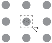
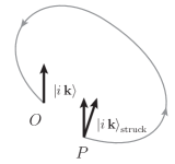
Figure 2.1: Left: Schematic illustration of our proposal to describe the electronic excitation induced by the struck nucleus located at $\mathbf{R}=\mathbf{0}$: only the initial states $\left\{\ket{\mathbf{0}\,m}\right\}$ are relevant for the excitation process and thus are subjected to the Galilean transformation $\hat{G}_{\mathbf{0}}\left(-\mathbf{q}_{e}\right)$. Right: Conceptual illustration of the evolution of Hamiltonian in parameter space (gray curve), with point $O$ ($P$) corresponding to the original (perturbed) Hamiltonian and relevant eigenstates $\left\{\ket{i\,\mathbf{k}}\right\}$ ($\left\{\left|i\,\mathbf{k}\right\rangle_{\mathrm{struck}}\right\}$). These two points are equivalent in the sense that they are connected to each other through an adiabatic evolution. See text for details.

In addition, since the timescale of the excitation is roughly $E_{g}^{-1}$, during which the recoiled nucleus at most travels a distance around $\left(q/m_{N}\right)E_{g}^{-1}\sim\mathcal{O}\left(10^{-2}\,\textrm{\AA}\right)$ for a momentum transfer $q\sim 1\,\mathrm{MeV}$, the excitation can be regarded as instantaneous, and thus the configuration effect of the displaced nucleus can be ignored.

3 Practical calculation of excitation event rates with WFs

3.1 Formalism

In this section we will derive the formalism of the excitation event rate induced by a recoiled nucleus in the bulk diamond. Here we consider a more realistic multiband case where a separate group of $J$ bands cross with each other, and a Bloch orbital can be expressed in terms of WFs $\left\{\ket{\mathbf{R}\,m}\right\}$ in following way:

$$\ket{i\,\mathbf{k}} = \sum_{\mathbf{R}}\frac{e^{i\mathbf{k}\cdot\mathbf{R}}}{\sqrt{N}}\left(\sum_{m=1}^{J}U_{mi}^{\left(\mathbf{k}\right)\dagger}\ket{\mathbf{R}\,m}\right),$$ (3.1)

and its inverse transformation

$$\ket{\mathbf{R}\,m} = \sum_{\mathbf{\mathbf{k}}}\frac{e^{-i\mathbf{k}\cdot\mathbf{R}}}{\sqrt{N}}\left(\sum_{i=1}^{J}U_{im}^{\left(\mathbf{k}\right)}\ket{i\,\mathbf{k}}\right),$$ (3.2)

with the unitary matrix $\mathbf{U}^{\left(\mathbf{k}\right)}$ that mixes different bands for each $\mathbf{k}$-vector. In practice, we use the code $\mathtt{Wannier\,90}$ MOSTOFI20142309 to realize this scheme, which specializes in constructing the maximally localized Wannier functions (MLWFs) from a set of Bloch states. To avoid distraction from present discussion, we arrange a short review of the MLWF in the Appendix A. In order to transplant the treatment on the Migdal effect applied in the isolated atom to the crystalline environment, the WFs are required to be atom-centered. Since there are two atoms in the unit cell of the crystalline diamond, here we introduce the Galilean boost operator $\hat{G}_{\mathbf{0}1}\left(\mathbf{q}_{e}\right)$ that accounts for recoil effect of the first diamond atom at the site $\left(\mathbf{R}=\mathbf{0},\,\bm{\tau}_{1}=\mathbf{0}\right)$, so one has the following transition amplitude $\left(i^{\prime}\neq i\right)$:

$$\left\langle i\,\mathbf{k}\right|\hat{G}_{\mathbf{0}1}\left(-\mathbf{q}_{e}\right)\left|i^{\prime}\,\mathbf{k}^{\prime}\right\rangle^{*} = \frac{1}{N}\sum_{m,m^{\prime}}\sum_{\mathbf{R}}U_{mi}^{\left(\mathbf{k}\right)\dagger}\left\langle\mathbf{R}\,m\right|\hat{G}_{\mathbf{0}1}\left(-\mathbf{q}_{e}\right)-\mathbf{1}\left|\mathbf{0}\,m^{\prime}\right\rangle^{*}\left(U_{m^{\prime}i^{\prime}}^{\left(\mathbf{k}^{\prime}\right)\dagger}\right)^{*}e^{i\mathbf{k}\cdot\mathbf{R}}$$ (3.3)

$$\simeq \frac{i}{N}\mathbf{q}_{e}\cdot\left(\sum_{m_{1},m}\sum_{\mathbf{R}}U_{i^{\prime}\,m_{1}}^{\left(\mathbf{k}^{\prime}\right)}\left\langle\mathbf{0}\,m_{1}\right|\hat{\mathbf{r}}\left|\mathbf{R}\,m\right\rangle U_{mi}^{\left(\mathbf{k}\right)\dagger}e^{i\mathbf{k}\cdot\mathbf{R}}\right)$$

$$= \frac{i}{N}\mathbf{q}_{e}\cdot\mathbf{J}_{1\left(i^{\prime}\mathbf{k}^{\prime};i\mathbf{k}\right)},$$

where the origin of coordinate operator $\hat{\mathbf{r}}$ is placed at the atom 1 in the unit cell, and the partial summation over $m_{1}$ corresponds to the WFs centered at atom 1. We use $\mathbf{J}_{1\left(i^{\prime}\mathbf{k}^{\prime};i\mathbf{k}\right)}$ to denote the summation in parenthesis in the second line. Since momentum transfer $\mathbf{q}$ is highly suppressed by $m_{e}/m_{N}$, in derivation we assume $\left|\mathbf{q}_{e}\right|\cdot\left|\mathbf{r}\right|\ll 1$, which is a good approximation for a sub-GeV DM. Similar discussion can be easily applied to the second atom located at $\bm{\tau}_{2}=\left(1/4,\,1/4,\,1/4\right)$, only keep in mind that the origin of operator $\hat{\mathbf{r}}$ is also placed at atom 1 in practical use of $\mathtt{Wannier\,90}$. After a translation, the corresponding transition amplitude for the atom 2 at the site $\mathbf{R}=\mathbf{0}$ is modified as

$$\left\langle i\,\mathbf{k}\right|\hat{G}_{\mathbf{0}2}\left(-\mathbf{q}_{e}\right)\left|i^{\prime}\,\mathbf{k}^{\prime}\right\rangle^{*} \simeq \frac{i}{N}\mathbf{q}_{e}\cdot\left(\sum_{m_{2},m}\sum_{\mathbf{R}}U_{i^{\prime}\,m_{2}}^{\left(\mathbf{k}^{\prime}\right)}\left\langle\mathbf{0}\,m_{2}\right|\hat{\mathbf{r}}\left|\mathbf{R}\,m\right\rangle U_{mi}^{\left(\mathbf{k}\right)\dagger}e^{i\mathbf{k}\cdot\mathbf{R}}-\mathbf{d}\sum_{m_{2}}U_{i^{\prime}\,m_{2}}^{\left(\mathbf{k}^{\prime}\right)}U_{m_{2}i}^{\left(\mathbf{k}\right)\dagger}\right)$$ (3.4)

$$= \frac{i}{N}\mathbf{q}_{e}\cdot\mathbf{J}_{2\left(i^{\prime}\mathbf{k}^{\prime};i\mathbf{k}\right)},$$

with $\mathbf{d}$ being the position vector of atom 2 relative to atom 1, and $\mathbf{J}_{2\left(i^{\prime}\mathbf{k}^{\prime};i\mathbf{k}\right)}$ encodes the terms in parenthesis. Thus, after taking into account the two degenerate spin states, the total excitation event rate can be expressed as

$$R = \frac{\rho_{\chi}}{m_{\chi}}\left(\frac{A^{2}\sigma_{\chi n}}{2\pi\mu_{\chi n}^{2}}\right)\left(\frac{m_{e}}{m_{N}}\right)^{2}\frac{V^{2}}{N}\int\mathrm{d}^{3}q\,\sum_{i^{\prime}}^{c}\sum_{i}^{v}\int_{1\mathrm{BZ}}\frac{\mathrm{d}^{3}k^{\prime}}{\left(2\pi\right)^{3}}\frac{\mathrm{d}^{3}k}{\left(2\pi\right)^{3}}\,\left\{\int\frac{g_{\chi}\left(\mathbf{w},\,\hat{\mathbf{q}}\right)}{q\,w}\,\mathrm{d}w\,\mathrm{d}\phi_{\mathbf{\hat{\mathbf{q}}}\mathbf{w}}\,\right.$$ (3.5)

$$\times\Theta\left[w-w_{\mathrm{min}}\left(q,\,E_{i^{\prime}\mathbf{k}^{\prime}}-E_{i\mathbf{k}}\right)\right]\,\left.\left(\left|\mathbf{q}\cdot\mathbf{J}_{1\left(i^{\prime}\mathbf{k}^{\prime};i\mathbf{k}\right)}\right|^{2}+\left|\mathbf{q}\cdot\mathbf{J}_{2\left(i^{\prime}\mathbf{k}^{\prime};i\mathbf{k}\right)}\right|^{2}\right)\right\},$$

where the sums are over the valence bands for initial states and the conducting bands for final states, respectively. For simplicity we approximate the velocity distribution as an isotropic one, and as a result the angular correlation between the laboratory velocity with respect to the galaxy and the orientation of the crystal is eliminated. Besides, in order to make the scan of parameters computationally more efficient, Eq. (3.5) can be further equivalently expressed as

$$R = \frac{\rho_{\chi}}{m_{\chi}}\left(\frac{A^{2}\sigma_{\chi n}\,q_{\mathrm{ref}}^{2}}{3\,\mu_{\chi n}^{2}}\right)\left(\frac{m_{e}}{m_{N}}\right)^{2}N\int\frac{4\pi g_{\chi}\left(w\right)}{w}\,\,\mathrm{d}w\int\mathrm{d}\ln E_{e}\,\mathrm{d}\ln q\,\,\Theta\left[w-w_{\mathrm{min}}\left(q,\,E_{e}\right)\right]\,\mathcal{F}\left(q,\,E_{e}\right),$$ (3.6)

where a momentum reference value is constructed as $q_{\mathrm{ref}}=2\pi/a$, and a non-dimensional crystal form factor is introduced as

$$\mathcal{F}\left(q,\,E_{e}\right) \equiv \left(\frac{q}{q_{\mathrm{ref}}}\right)^{2}\sum_{i^{\prime}}^{c}\sum_{i}^{v}\int_{1\mathrm{BZ}}\frac{\varOmega\,\mathrm{d}^{3}k^{\prime}}{\left(2\pi\right)^{3}}\frac{\varOmega\,\mathrm{d}^{3}k}{\left(2\pi\right)^{3}}\,\left[E_{e}\,\delta\left(E_{i^{\prime}\mathbf{k}^{\prime}}-E_{i\mathbf{k}}-E_{e}\right)\,q^{2}\left(\left|\mathbf{J}_{1\left(i^{\prime}\mathbf{k}^{\prime};i\mathbf{k}\right)}\right|^{2}+\left|\mathbf{J}_{2\left(i^{\prime}\mathbf{k}^{\prime};i\mathbf{k}\right)}\right|^{2}\right)\right].$$ (3.7)

Specifically, after inserting the monochromatic velocity distribution $4\pi g_{\chi}\left(v\right)=\delta\left(v-w\right)$ the total transition rate for parameter pair $(m_{\chi},\,w)$ can be recast as

$$R\left(m_{\chi},\,w\right) = \frac{\rho_{\chi}}{m_{\chi}}\left(\frac{A^{2}\sigma_{\chi n}\,q_{\mathrm{ref}}^{2}}{3\,w\,\mu_{\chi n}^{2}}\right)\left(\frac{m_{e}}{m_{N}}\right)^{2}N\int\mathrm{d}\ln E_{e}\,\mathrm{d}\ln q\,\Theta\left[w-w_{\mathrm{min}}\left(q,\,E_{e}\right)\right]\,\mathcal{F}\left(q,\,E_{e}\right).$$ (3.8)

3.2 Computational details and results

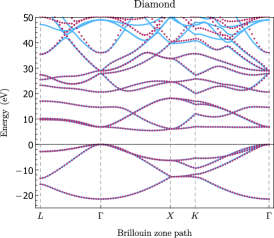
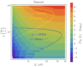
Figure 3.1: Left: The band structures of bulk crystalline diamond obtained from DFT calculation (blue solid line) and Wannier interpolation (red dotted line). Right: The crystal form function $\mathcal{F}\left(q,\,E_{e}\right)$. The area contoured in yellow (blue) represents the parameter region relevant for the Migdal excitation event rate for parameter $m_{\chi}=500\,\mathrm{MeV}$, $w=100\,\mathrm{km/s}$ ($m_{\chi}=10\,\mathrm{MeV}$, $w=800\,\mathrm{km/s}$). See text for details.

Now we put into practice the estimate of the Migdal excitation event rate. With $\mathtt{Quantum\,Espresso}$ code Giannozzi_2009 , we first perform the DFT calculation to obtain the Bloch eigenfunctions and eigenvalues using the plane-wave basis set and Troullier-Martins norm-conserving (NC) pseudopotentials in the Kleinman-Bylander representation, on a 20$\times$20$\times$20 Monkhorst-Pack mesh of $k$-points. The exchange-correlation functional is treated within the generalized gradient approximation (GGA) parametrized by Perdew, Burke, and Ernzerhof (PBE) PhysRevLett.77.3865 . The energy cut is set to $90$ Ry and a lattice constant $a=3.560$ Å  obtained from relaxation is adopted.

Then we invoke the software package $\mathtt{Wannier\,90}$ MOSTOFI20142309 to compute the matrix element $\left\langle\mathbf{0}\,m^{\prime}\right|\hat{\mathbf{r}}\left|\mathbf{R}\,m\right\rangle$ and the unitary matrix $\mathbf{U}^{\left(\mathbf{k}\right)}$ using a smaller homogeneous set of 16$\times$16$\times$16 $k$-points. We generate $J=32$ WFs out of $\mathcal{J}_{\mathbf{k}}=72$ Bloch wavefunctions from the DFT calculation by beginning with a set of 32 localized trial orbitals $\left\{g_{n}\left(\mathbf{r}\right)\right\}$ that correspond to $s$, $p$, $d$, $f$ orbitals as some rough initial guess for these WFs. In order to fix the WFs at the atom while containing their spreads, the gauge selection step is expediently spared because otherwise some MLWFs will be found located at interstitial sites, which makes the picture of recoiled atom ambiguous. The widest spread of these generated WFs is around $\left(1.4\,\textrm{\AA}\right)^{2}$, so hopping terms within up to the third neighbor unit cells are sufficient to guarantee convergence in calculation of $\left\langle\mathbf{0}\,m^{\prime}\right|\hat{\mathbf{r}}\left|\mathbf{R}\,m\right\rangle$.

On the other hand, once a set of localized WFs have been determined, and hence the Hamiltonian matrices $\left\langle\mathbf{R}\,m\right|\hat{H}\left|\mathbf{0}\,m^{\prime}\right\rangle$ are tabulated, the band structures become an eigenvalue problem

$$\sum_{m^{\prime}=1}^{J}\sum_{\mathbf{R}}\left\langle\mathbf{R}\,m\right|\hat{H}\left|\mathbf{0}\,m^{\prime}\right\rangle e^{-i\mathbf{k}\cdot\mathbf{R}}\,U_{m^{\prime}i}^{\left(\mathbf{k}\right)\dagger} = \bar{\epsilon}_{i\,\mathbf{k}}\,U_{mi}^{\left(\mathbf{k}\right)\dagger},$$ (3.9)

where the eigenvalue $\bar{\epsilon}_{i\,\mathbf{k}}$ corresponds to the $i$-th band energy at $\mathbf{k}$, and the eigenvectors $U_{mi}^{\left(\mathbf{k}\right)\dagger}$ that form a $J\times J$ unitary matrix are deliberately written in accordance with Eq. (3.1). Such procedure is called the Wannier interpolation. The band structures of crystalline diamond from the DFT calculation and interpolation are presented in the left panel of Fig. 3.1, where the blue solid line (red dotted line) represents the DFT calculation (Wannier interpolation). To reproduce exactly the original DFT band structures in a specific energy range, Bloch states spanning relevant range are faithfully retained in the subspace selection procedure, and such energy range is referred to as “frozen energy window”, or “inner window”. In this work, we choose a frozen energy window ranging from the bottom of the valence band to 40 eV above the valence band maximums, which is also reflected in Fig. 3.1.

In practical computation of the form factor Eq. (3.7) we use a bin width $\Delta E=0.059\,\mathrm{eV}$ to smear the delta function, and the integrand is evaluated at the central value in each energy bin. Besides, the integrals of the continuous $k$-points in the 1BZ are replaced by corresponding summations over the uniform 16$\times$16$\times$16 $k$-points. In the right panel of Fig. 3.1 shown is the crystal form factor $\mathcal{F}\left(q,\,E_{e}\right)$ introduced in Eq. (3.7), where momentum transfer $q$ is expressed in terms of the diamond reciprocal lattice $2\pi/a\approx 3.48\,\mathrm{keV}$. For demonstration, we choose two benchmark pairs of parameters $\left(m_{\chi},\,w\right)$ to calculate the transition event rate in Eq. (3.8). Due to the step function that embodies the kinetic constraint, only the areas enclosed in the contours contribute to the excitation event rate. For example, when a cross section $\sigma_{\chi n}=10^{-38}\,\mathrm{cm}^{2}$ is assumed, parameters $m_{\chi}=500\,\mathrm{MeV},\>w=100\,\mathrm{km/s}$ presented in yellow corresponds to an excitation event rate of $0.027\,/\mathrm{kg/yr}$, while $m_{\chi}=10\,\mathrm{MeV},\>w=800\,\mathrm{km/s}$ in blue corresponds to an excitation event rate of $0.299\,\mathrm{/kg/yr}$. It is noted that although a heavier DM tends to prompt a larger momentum transfer and hence results in a larger transition probability, a suppression factor inversely proportional to $m_{\chi}^{3}$ may alleviate or even offset such mass effect in the sub-GeV mass range, depending on velocity.

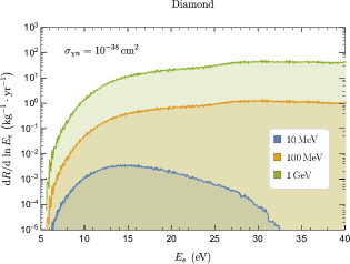
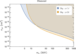
Figure 3.2: Left: The differential electronic excitation event rate of the Migdal effect in crystalline diamond for reference values $\sigma_{\chi n}=10^{-38}\,\mathrm{cm}^{2}$ and $m_{\chi}=10\,\mathrm{MeV}$ (blue), $100\,\mathrm{MeV}$(orange) and $1\,\mathrm{GeV}$ (green), respectively. Right: Cross-section sensitivities for the Migdal effect at 90% C.L. for a 1 kg-yr diamond detector, based on a single-electron (blue) and a two-electron (orange) signals, respectively. See text for details.

In left panel of Fig. 3.2 we plot the velocity-averaged energy spectra of the Migdal excitation for DM mass $m_{\chi}=10\,\mathrm{MeV}$ (blue), $100\,\mathrm{MeV}$(orange) and $1\,\mathrm{GeV}$ (green), respectively. It is observed that these spectra do not fall off as quickly as the case in direct DM-electron excitation process calculated in Ref. Essig:2015cda . Hence a wider energy range is usually required to fully describe the Migdal effect in crystalline environment. From the energy spectra we also estimate the sensitivity of 1 kg-yr exposure of diamond detector in the right panel of Fig. 3.2, assuming an average energy of $13\,\mathrm{eV}$ for producing one electron-hole pair Kurinsky:2019pgb . The 90% C.L. exclusion contours for DM-nucleon cross section for both the single-electron (blue) and the two-electron (orange) bins are presented with no background event assumed.

4 Summary and discussions

In this paper we presented a tight-binding approach to describe the Migdal effect in the diamond crystal. This localized description is a natural choice to generalize the well established treatment for isolated atoms to the case in crystalline solids. To achieve such TB description we generate a set of atom-centered WFs by use of software packages $\mathtt{Quantum\,Espresso}$ and $\mathtt{Wannier\,90}$. While the localization effect of the recoiled atom is preserved in forms of WFs, the delocalized nature of the Bloch states in solids is encoded in the hopping terms at the same time. Based on these hopping integrals, the electronic excitation rates induced by the recoiled ion were computed straightforwardly.

Here we make some comments on our methodology. As has been noted in previous section, our method deviates a little from the standard procedure to derive the MLWFs implemented in $\mathtt{Wannier\,90}$, which usually includes two steps, namely, subspace selection and gauge selection. The latter step is skipped in our computation so as to restrict the centers of WFs to the lattice sites. As a consequence, the spreads of those WFs have not been optimally minimized. From a conceptual point of view, this does not cause a severe problem because although WFs indicate some atomic properties and provide intuitive pictures of the chemical bonds, they do not necessarily bear definite physical meanings such as real atomic wavefunctions in solids. Actually, to determine the WFs is experimentally infeasible, even in principle RevModPhys.84.1419 . In this sense, even a set of relatively “fat” WFs suffice in calculation of the excitation event rate, as long as sufficiently large number of neighbors are included in hopping integrals. However, WFs with too large spreads indeed cause inconvenience in practice. This partly explains why we choose diamond crystal rather than other tetrahedral semiconductors as example to describe the Migdal effect in semiconductors: for the cases of silicon and germanium, $\mathtt{Wannier\,90}$ is found to generate atom-centered WFs with much larger spreads in the same energy window unless a gauge optimization is performed, and hence more computational efforts are required to reach convergence.

Another concern is how the calculation of Migdal excitation rates will rely on the selection of the WFs, considering there existing a gauge freedom in the unitary matrix $\mathbf{U}^{\left(\mathbf{k}\right)}$ in Eq. (3.2). In fact, since it is required that the centers of the WFs locate at the lattice sites to account for the struck atoms, such invariance of arbitrary WF selection is unnecessary in formulating the transition probability. To see this, recall the transition amplitude in Eq. (3.3), while the initial state $\sum\limits_{m,\mathbf{R}}e^{i\mathbf{k}\cdot\mathbf{R}}\left|\mathbf{R}\,m\right\rangle U_{mi}^{\left(\mathbf{k}\right)\dagger}\propto\left|i\,\mathbf{k}\right\rangle$ as a whole is independent of the WFs, the conduction final part $\sum\limits_{m_{1}}U_{i^{\prime}\,m_{1}}^{\left(\mathbf{k}^{\prime}\right)}\left\langle\mathbf{0}\,m_{1}\right|$ is invariant only within the WF subspace attached to atom 1. This can be understood intuitively with the example of tetrahedral $sp^{3}$ hybridization, where the valence wavefunctions around an atom can be expressed either as linear combinations of $s$ and $p$ atomic orbitals, or combinations of four identical $sp$-hybrid orbitals pointing along the directions from the center to the corners of a tetrahedron. All these different choices should keep the sum $\sum\limits_{m_{1}}U_{i^{\prime}\,m_{1}}^{\left(\mathbf{k}^{\prime}\right)}\left\langle\mathbf{0}\,m_{1}\right|$ invariant. To verify this, we used $s$, $p$ atomic orbitals and $sp^{3}$ hybrids among other orbitals as trial wavefunctions $\left\{g_{n}\left(\mathbf{r}\right)\right\}$ to wannierize and calculate the transition event rate respectively, and the difference between the two results turns out to be well within a few percent, indicating a good agreement. Thus our approach has proved both effective and self-consistent.

Appendix A Maximally localized Wannier functions

Since our practical realization of the atom-centered WFs is closely related to the generation of the maximally localized Wannier functions  (MLWFs) via implementing software $\mathtt{Wannier\,90}$ MOSTOFI20142309 , here we take a brief review. From Eq. (3.2) it is straightforward to see that the WFs are non-unique due to the arbitrariness of the unitary matrix $\mathbf{U}^{\left(\mathbf{k}\right)}$. In order to overcome such indeterminacy, Mazari and Vanderbilt PhysRevB.56.12847 developed a procedure to minimize the second moment of the WFs around their centers so as to generate a set of well-defined and localized WFs, namely, the maximally localized Wannier functions. Given an isolated group of $J$ Bloch bands, the procedure begins with a set of $J$ localized trial orbitals $\left\{g_{n}\left(\mathbf{r}\right)\right\}$ as some rough initial guess for corresponding WFs, which are then projected onto those Bloch wavefunctions as the following,

$$\left|\phi_{n\mathbf{k}}\right\rangle = \sum_{i=1}^{J}\left|i\,\mathbf{k}\right\rangle\braket{i\,\mathbf{k}}{g_{n}},$$ (A.1)

which are typically smooth in $\mathbf{k}$ and hence are well-localized in space. By further Löwdin-orthonormalizing these functions one obtains $J$ Bloch-like states $\widetilde{\left|i\,\mathbf{k}\right\rangle}$ that are related to the original $\left|i\,\mathbf{k}\right\rangle$ via a $J\times J$ unitary matrix $U_{\mathbf{k}}$ in the following manner,

$$\widetilde{\left|i\,\mathbf{k}\right\rangle} = \sum_{j=1}^{J}\left|j\,\mathbf{k}\right\rangle U_{\mathbf{k},ij}.$$ (A.2)

Substituting $\left|i\,\mathbf{k}\right\rangle$ in Eq. (2.6) with $\widetilde{\left|i\,\mathbf{k}\right\rangle}$ we then have $J$ localized WFs. The minimization criterion proposed by Mazari and Vanderbilt mentioned above is to minimize the functional

$$\Omega = \sum_{n}\left[\left\langle\mathbf{0}\,n\right|\hat{r}^{2}\left|\mathbf{0}\,n\right\rangle-\left|\left\langle\mathbf{0}\,n\right|\hat{\mathbf{r}}\left|\mathbf{0}\,n\right\rangle\right|^{2}\right]$$ (A.3)

$$= \varOmega_{\mathrm{I}}+\tilde{\varOmega},$$

with

$$\varOmega_{\mathrm{I}} = \sum_{n}\left[\left\langle\mathbf{0}\,n\right|\hat{r}^{2}\left|\mathbf{0}\,n\right\rangle-\sum_{\mathbf{R},m}\left|\left\langle\mathbf{R}\,m\right|\hat{\mathbf{r}}\left|\mathbf{0}\,n\right\rangle\right|^{2}\right]$$ (A.4)

and

$$\tilde{\varOmega} = \sum_{n}\,\sum_{\mathbf{R}m\neq\mathbf{0}n}\left|\left\langle\mathbf{R}\,m\right|\hat{\mathbf{r}}\left|\mathbf{0}\,n\right\rangle\right|^{2}.$$ (A.5)

The purpose of such separation is that $\varOmega_{\mathrm{I}}$ is invariant under arbitrary unitary transformation $\mathbf{U}^{\left(\mathbf{k}\right)}$ in Eq. (3.2), and hence the minimization of $\Omega$ depends only on the variation effects of gauge $\mathbf{U}^{\left(\mathbf{k}\right)}$ on the term $\tilde{\varOmega}$. Since the matrix $U_{\mathbf{k}}$ in Eq. (A.2) has already provided $J$ sufficiently localized WFs, we use them as the starting point for the iterative steepest-descent method to reach the optimal unitary transformation $\mathbf{U}^{\left(\mathbf{k}\right)}$ that minimizes $\tilde{\varOmega}$. This procedure is called gauge selection.

In more general cases, additional modifications are required to pick the Bloch orbitals of interest from those unwanted ones when the bands are crossing with each other. The Souza-Marzari-Vanderbilt method proposed in Ref. PhysRevB.65.035109 successfully realized such disentanglement. In this approach, one first identifies a set of $\mathcal{J}_{\mathbf{k}}\geq J$ Bloch orbitals that form a $\mathcal{J}_{\mathbf{k}}$-dimensional Hilbert space at each point $\mathbf{k}$ in the 1BZ in a sufficiently large energy range, which is dubbed as “disentanglement window”, or “outer window”, and then chooses a $J$-dimensional subspace that gives the smallest possible value of $\varOmega_{\mathrm{I}}$ via iterative procedures. Similarly to above discussion, the minimization of $\varOmega_{\mathrm{I}}$ also begins with a rough initial guess that are usually obtained by first projecting $J$ localized trial orbitals $\left\{g_{n}\left(\mathbf{r}\right)\right\}$ onto $\mathcal{J}_{\mathbf{k}}$ Bloch states such that

$$\left|\phi_{n\mathbf{k}}\right\rangle = \sum_{j=1}^{\mathcal{J}_{\mathbf{k}}}\left|j\,\mathbf{k}\right\rangle\braket{j\,\mathbf{k}}{g_{n}},$$ (A.6)

and then constructing the following $J$ orthonormalized Bloch-like states $\widetilde{\left|i\,\mathbf{k}\right\rangle}$ that are related to the original $\left|i\,\mathbf{k}\right\rangle$ via a $\mathcal{J}_{\mathbf{k}}\times J$ matrix $V_{\mathbf{k}}$ such as

$$\widetilde{\left|i\,\mathbf{k}\right\rangle} = \sum_{j=1}^{\mathcal{J}_{\mathbf{k}}}\left|j\,\mathbf{k}\right\rangle V_{\mathbf{k},ij}.$$ (A.7)

An algebraic algorithm that updates the minimization iteratively is then used to obtained $J$-dimensional optimal subspace in a self-consistent manner. This process is called subspace selection. Once the optimal subspace is determined, i.e., the minimization of $\varOmega_{\mathrm{I}}$ is achieved, the gauge-selection step to further minimize the noninvariant part $\tilde{\varOmega}$ follows, until a set of self-consistent MLWFs are obtained.

References

- (1) XENON collaboration, Dark Matter Search Results from a One Ton-Year Exposure of XENON1T, Phys. Rev. Lett. 121 (2018) 111302 [1805.12562].
- (2) XENON collaboration, Light Dark Matter Search with Ionization Signals in XENON1T, 1907.11485.
- (3) LUX collaboration, Results of a Search for Sub-GeV Dark Matter Using 2013 LUX Data, Phys. Rev. Lett. 122 (2019) 131301 [1811.11241].
- (4) PandaX-II collaboration, Constraining Dark Matter Models with a Light Mediator at the PandaX-II Experiment, Phys. Rev. Lett. 121 (2018) 021304 [1802.06912].
- (5) SuperCDMS collaboration, Low-mass dark matter search with CDMSlite, Phys. Rev. D97 (2018) 022002 [1707.01632].
- (6) CDEX collaboration, Constraints on Spin-Independent Nucleus Scattering with sub-GeV Weakly Interacting Massive Particle Dark Matter from the CDEX-1B Experiment at the China Jinping Underground Laboratory, Phys. Rev. Lett. 123 (2019) 161301 [1905.00354].
- (7) CRESST collaboration, First results from the CRESST-III low-mass dark matter program, 1904.00498.
- (8) DarkSide collaboration, Low-Mass Dark Matter Search with the DarkSide-50 Experiment, Phys. Rev. Lett. 121 (2018) 081307 [1802.06994].
- (9) EDELWEISS collaboration, Searching for low-mass dark matter particles with a massive Ge bolometer operated above-ground, Phys. Rev. D99 (2019) 082003 [1901.03588].
- (10) R. Essig, J. Mardon and T. Volansky, Direct Detection of Sub-GeV Dark Matter, Phys. Rev. D85 (2012) 076007 [1108.5383].
- (11) P. W. Graham, D. E. Kaplan, S. Rajendran and M. T. Walters, Semiconductor Probes of Light Dark Matter, Phys. Dark Univ. 1 (2012) 32 [1203.2531].
- (12) R. Essig, M. Fernandez-Serra, J. Mardon, A. Soto, T. Volansky and T.-T. Yu, Direct Detection of sub-GeV Dark Matter with Semiconductor Targets, JHEP 05 (2016) 046 [1509.01598].
- (13) Y. Hochberg, T. Lin and K. M. Zurek, Absorption of light dark matter in semiconductors, Phys. Rev. D95 (2017) 023013 [1608.01994].
- (14) Y. Hochberg, Y. Zhao and K. M. Zurek, Superconducting Detectors for Superlight Dark Matter, Phys. Rev. Lett. 116 (2016) 011301 [1504.07237].
- (15) Y. Hochberg, T. Lin and K. M. Zurek, Detecting Ultralight Bosonic Dark Matter via Absorption in Superconductors, Phys. Rev. D94 (2016) 015019 [1604.06800].
- (16) Y. Hochberg, Y. Kahn, M. Lisanti, K. M. Zurek, A. G. Grushin, R. Ilan et al., Detection of sub-MeV Dark Matter with Three-Dimensional Dirac Materials, Phys. Rev. D97 (2018) 015004 [1708.08929].
- (17) A. Coskuner, A. Mitridate, A. Olivares and K. M. Zurek, Directional Dark Matter Detection in Anisotropic Dirac Materials, 1909.09170.
- (18) R. M. Geilhufe, F. Kahlhoefer and M. W. Winkler, Dirac Materials for Sub-MeV Dark Matter Detection: New Targets and Improved Formalism, 1910.02091.
- (19) S. Knapen, T. Lin and K. M. Zurek, Light Dark Matter in Superfluid Helium: Detection with Multi-excitation Production, Phys. Rev. D95 (2017) 056019 [1611.06228].
- (20) A. Caputo, A. Esposito and A. D. Polosa, Sub-MeV Dark Matter and the Goldstone Modes of Superfluid Helium, 1907.10635.
- (21) A. Caputo, A. Esposito, E. Geoffray, A. D. Polosa and S. Sun, Dark Matter, Dark Photon and Superfluid He-4 from Effective Field Theory, 1911.04511.
- (22) S. Knapen, T. Lin, M. Pyle and K. M. Zurek, Detection of Light Dark Matter With Optical Phonons in Polar Materials, Phys. Lett. B785 (2018) 386 [1712.06598].
- (23) S. Griffin, S. Knapen, T. Lin and K. M. Zurek, Directional Detection of Light Dark Matter with Polar Materials, Phys. Rev. D98 (2018) 115034 [1807.10291].
- (24) B. Campbell-Deem, P. Cox, S. Knapen, T. Lin and T. Melia, Multiphonon excitations from dark matter scattering in crystals, 1911.03482.
- (25) R. Essig, A. Manalaysay, J. Mardon, P. Sorensen and T. Volansky, First Direct Detection Limits on sub-GeV Dark Matter from XENON10, Phys. Rev. Lett. 109 (2012) 021301 [1206.2644].
- (26) S. K. Lee, M. Lisanti, S. Mishra-Sharma and B. R. Safdi, Modulation Effects in Dark Matter-Electron Scattering Experiments, Phys. Rev. D92 (2015) 083517 [1508.07361].
- (27) Y. Hochberg, M. Pyle, Y. Zhao and K. M. Zurek, Detecting Superlight Dark Matter with Fermi-Degenerate Materials, JHEP 08 (2016) 057 [1512.04533].
- (28) I. M. Bloch, R. Essig, K. Tobioka, T. Volansky and T.-T. Yu, Searching for Dark Absorption with Direct Detection Experiments, JHEP 06 (2017) 087 [1608.02123].
- (29) S. Derenzo, R. Essig, A. Massari, A. Soto and T.-T. Yu, Direct Detection of sub-GeV Dark Matter with Scintillating Targets, Phys. Rev. D96 (2017) 016026 [1607.01009].
- (30) Y. Hochberg, Y. Kahn, M. Lisanti, C. G. Tully and K. M. Zurek, Directional detection of dark matter with two-dimensional targets, Phys. Lett. B772 (2017) 239 [1606.08849].
- (31) R. Essig, J. Mardon, O. Slone and T. Volansky, Detection of sub-GeV Dark Matter and Solar Neutrinos via Chemical-Bond Breaking, Phys. Rev. D95 (2017) 056011 [1608.02940].
- (32) F. Kadribasic, N. Mirabolfathi, K. Nordlund, A. E. Sand, E. Holmstrom and F. Djurabekova, Directional Sensitivity In Light-Mass Dark Matter Searches With Single-Electron Resolution Ionization Detectors, Phys. Rev. Lett. 120 (2018) 111301 [1703.05371].
- (33) R. Essig, T. Volansky and T.-T. Yu, New Constraints and Prospects for sub-GeV Dark Matter Scattering off Electrons in Xenon, Phys. Rev. D96 (2017) 043017 [1703.00910].
- (34) A. Arvanitaki, S. Dimopoulos and K. Van Tilburg, Resonant absorption of bosonic dark matter in molecules, Phys. Rev. X8 (2018) 041001 [1709.05354].
- (35) R. Budnik, O. Chesnovsky, O. Slone and T. Volansky, Direct Detection of Light Dark Matter and Solar Neutrinos via Color Center Production in Crystals, Phys. Lett. B782 (2018) 242 [1705.03016].
- (36) P. Sharma, Role of nuclear charge change and nuclear recoil on shaking processes and their possible implication on physical processes, Nuclear Physics A 968 (2017) 326 .
- (37) G. Cavoto, F. Luchetta and A. D. Polosa, Sub-GeV Dark Matter Detection with Electron Recoils in Carbon Nanotubes, Phys. Lett. B776 (2018) 338 [1706.02487].
- (38) Z.-L. Liang, L. Zhang, P. Zhang and F. Zheng, The wavefunction reconstruction effects in calculation of DM-induced electronic transition in semiconductor targets, JHEP 01 (2019) 149 [1810.13394].
- (39) M. Heikinheimo, K. Nordlund, K. Tuominen and N. Mirabolfathi, Velocity Dependent Dark Matter Interactions in Single-Electron Resolution Semiconductor Detectors with Directional Sensitivity, Phys. Rev. D99 (2019) 103018 [1903.08654].
- (40) T. Trickle, Z. Zhang, K. M. Zurek, K. Inzani and S. Griffin, Multi-Channel Direct Detection of Light Dark Matter: Theoretical Framework, 1910.08092.
- (41) T. Trickle, Z. Zhang and K. M. Zurek, Direct Detection of Light Dark Matter with Magnons, 1905.13744.
- (42) R. Catena, T. Emken, N. Spaldin and W. Tarantino, Atomic responses to general dark matter-electron interactions, 1912.08204.
- (43) M. Ibe, W. Nakano, Y. Shoji and K. Suzuki, Migdal effect in dark matter direct detection experiments, Journal of High Energy Physics 2018 (2018) 194.
- (44) R. Bernabei et al., On electromagnetic contributions in WIMP quests, Int. J. Mod. Phys. A22 (2007) 3155 [0706.1421].
- (45) M. J. Dolan, F. Kahlhoefer and C. McCabe, Directly detecting sub-GeV dark matter with electrons from nuclear scattering, Phys. Rev. Lett. 121 (2018) 101801 [1711.09906].
- (46) N. F. Bell, J. B. Dent, J. L. Newstead, S. Sabharwale and T. J. Weiler, The Migdal Effect and Photon Bremsstrahlung in effective field theories of dark matter direct detection and coherent elastic neutrino-nucleus scattering, 1905.00046.
- (47) D. Baxter, Y. Kahn and G. Krnjaic, Electron Ionization via Dark Matter-Electron Scattering and the Migdal Effect, 1908.00012.
- (48) T. Emken, R. Essig, C. Kouvaris and M. Sholapurkar, Direct Detection of Strongly Interacting Sub-GeV Dark Matter via Electron Recoils, JCAP 1909 (2019) 070 [1905.06348].
- (49) R. Essig, J. Pradler, M. Sholapurkar and T.-T. Yu, On the relation between Migdal effect and dark matter-electron scattering in atoms and semiconductors, 1908.10881.
- (50) N. Marzari, A. A. Mostofi, J. R. Yates, I. Souza and D. Vanderbilt, Maximally localized wannier functions: Theory and applications, Rev. Mod. Phys. 84 (2012) 1419.
- (51) A. Ambrosetti and P. L. Silvestrelli, Introduction to Maximally Localized Wannier Functions, ch. 6, pp. 327–368. John Wiley & Sons, Ltd, 2016. https://onlinelibrary.wiley.com/doi/pdf/10.1002/9781119148739.ch6. 10.1002/9781119148739.ch6.
- (52) H. Schober, An introduction to the theory of nuclear neutron scatterin in condensed matter, Journal of Neutron Research (2014) 109.
- (53) K. Schutz and K. M. Zurek, Detectability of Light Dark Matter with Superfluid Helium, Phys. Rev. Lett. 117 (2016) 121302 [1604.08206].
- (54) F. Acanfora, A. Esposito and A. D. Polosa, Sub-GeV Dark Matter in Superfluid He-4: an Effective Theory Approach, Eur. Phys. J. C79 (2019) 549 [1902.02361].
- (55) N. A. Kurinsky, T. C. Yu, Y. Hochberg and B. Cabrera, Diamond Detectors for Direct Detection of Sub-GeV Dark Matter, Phys. Rev. D99 (2019) 123005 [1901.07569].
- (56) P. Giannozzi, S. Baroni, N. Bonini, M. Calandra, R. Car, C. Cavazzoni et al., QUANTUM ESPRESSO: a modular and open-source software project for quantum simulations of materials, Journal of Physics: Condensed Matter 21 (2009) 395502.
- (57) A. A. Mostofi, J. R. Yates, G. Pizzi, Y.-S. Lee, I. Souza, D. Vanderbilt et al., An updated version of wannier90: A tool for obtaining maximally-localised wannier functions, Computer Physics Communications 185 (2014) 2309 .
- (58) J. P. Perdew, K. Burke and M. Ernzerhof, Generalized gradient approximation made simple, Phys. Rev. Lett. 77 (1996) 3865.
- (59) N. Marzari and D. Vanderbilt, Maximally localized generalized wannier functions for composite energy bands, Phys. Rev. B 56 (1997) 12847.
- (60) I. Souza, N. Marzari and D. Vanderbilt, Maximally localized wannier functions for entangled energy bands, Phys. Rev. B 65 (2001) 035109.