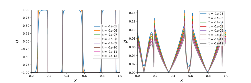
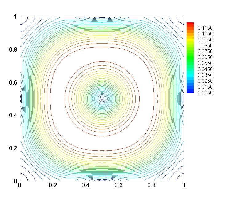
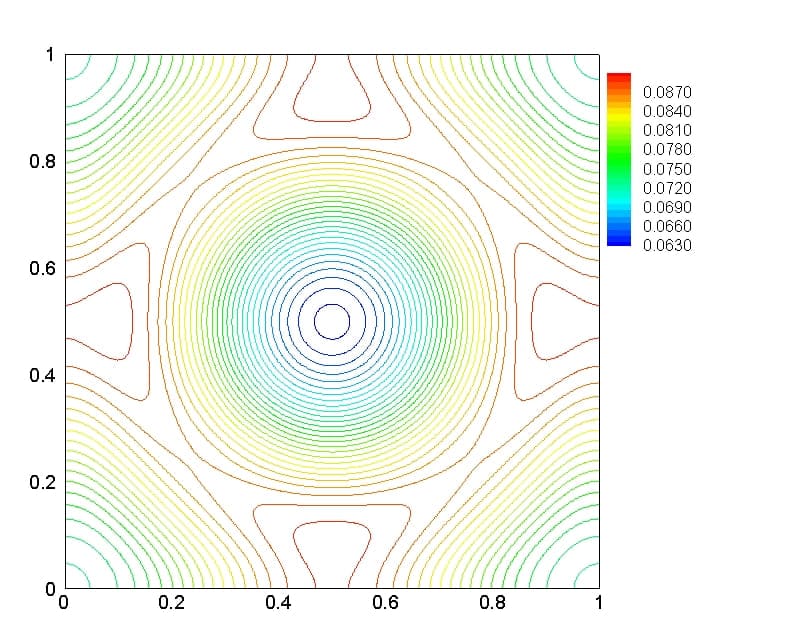
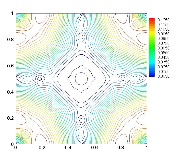
11footnotetext: Laboratoire Jacques-Louis Lions & Centre National de la Recherche Scientifique, Sorbonne Université, 4 Place Jussieu, 75252 Paris, France. Email: caoy@ljll.math.upmc.fr, contact@philippelefloch.org.
2 Department of Civil Engineering, University of Ottawa, Ottawa, ON K1N 6N5, Canada. Email: sghaz023@uottawa.ca. Key Words and Phrases. Cosmological Euler model; shock wave; asymptotic structure; finite volume scheme; geometry-preserving; high-order accuracy.

Asymptotic structure of cosmological fluid flows in one
and two space dimensions: a numerical study

Yangyang Cao1, Mohammad A. Ghazizadeh2, and Philippe G. LeFloch1
(December 2019)
Abstract

We consider an isothermal compressible fluid evolving on a cosmological background which may be either expanding or contracting toward the future. The Euler equations governing such a flow consist of two nonlinear hyperbolic balance laws which we treat in one and in two space dimensions. We design a finite volume scheme which is fourth-order accurate in time and second-order accurate in space. This scheme allows us to compute weak solutions containing shock waves and, by design, is well-balanced in the sense that it preserves exactly a special class of solutions. Using this scheme, we investigate the asymptotic structure of the fluid when the time variable approaches infinity (in the expanding regime) or approaches zero (in the contracting regime). We study these two limits by introducing a suitable rescaling of the density and velocity variables and, in turn, we analyze the effects induced by the geometric terms (of expanding or contracting nature) and the nonlinear interactions between shocks. Extensive numerical experiments in one and in two space dimensions are performed in order to support our observations.

1 Introduction

One of the challenges we address in this paper is the design of a geometry-preserving method that accurately compute fluid flows in presence of non-homogeneous geometrical effects. We build upon earlier work on structure-preserving numerical methods for nonlinear hyperbolic problems, for instance in Chertock et al. [10], Michel-Dansac et al. [21], and Russo [22, 23] and the many references cited therein. Specifically, we are interested in the global dynamics of compressible relativistic fluids evolving on a curved cosmological background of expanding or contracting type. Our model is essentially the Euler system posed on a FLRW background (after Friedmann–Lemaître–Robertson–Walker) and describe fluids evolving on a homogeneous and isotropic cosmology. Recall that shock wave solutions to nonlinear hyperbolic equations (such as the Euler equations) are defined in the forward time direction only and, since the geometry under consideration is singular at the time normalized to be t=0𝑡0t=0, we distinguish between two formulations of the initial value problem, corresponding to different ranges of the time variable.

In the range t(0,+)𝑡0t\in(0,+\infty), the background is expanding toward the future and a defining geometric coefficient a=a(t)𝑎𝑎𝑡a=a(t) (related to the speed of cosmological expansion or contraction, introduced below) increases monotonically to ++\infty. In this regime, we prescribe the initial data at some positive time t0>0subscript𝑡00t_{0}>0. On the other hand, in the range t(,0)𝑡0t\in(-\infty,0), the background is contracting toward the future and the coefficient a=a(t)𝑎𝑎𝑡a=a(t) decreases monotonically until it reaches a(0)=0𝑎00a(0)=0. In this regime, we prescribe the initial data at some negative t0<0subscript𝑡00t_{0}<0. A typical choice for the defining geometric coefficient is the function a(t)=a0(t/t0)α𝑎𝑡subscript𝑎0superscript𝑡subscript𝑡0𝛼a(t)=a_{0}(t/t_{0})^{\alpha}, often normalized by taking a0=1subscript𝑎01a_{0}=1 and t0=±1subscript𝑡0plus-or-minus1t_{0}=\pm 1 and for some rate of contraction/expansion α(0,1)𝛼01\alpha\in(0,1). In our study, we also allow the background spacetime to be spatially non-homogeneous.

Our aim is to design a numerical algorithm adapted to this problem and based on the finite volume methodology, and next to investigate the late-time asymptotics of solutions in the expanding direction as well as the behavior of the flow as one approaches the cosmological singularity. The model of interest here is given by the Euler equations and, for the sake of simplicity, the fluid sound speed is assumed to be a constant. By distinguishing between two cases, whether the background is expanding or contracting toward the future, we find that a fine structure arises which consists of non-interacting shock waves that move periodically in time. Importantly, our scheme is sufficiently robust so that this fine structure is correctly captured by our algorithm at a reasonable computational cost. The proposed method relies on a high-order Runge-Kutta discretization in the time variable and a structure-preserving technique for the spatial discretization.

Our aim is to investigate the fine structure of the solutions in the expanding direction t+𝑡t\to+\infty as well as in the contracting direction t0𝑡0t\to 0. We expect that the flow structure will somehow “simplifies” asymptotically, and we are interested in the competition taking place between the shock propagation and the background geometry. By working with periodic boundary conditions, we expect that the shocks will interact until only a simple pattern is left, typically the so-called N𝑁N-wave profile that is well-known for nonlinear systems of conservation laws. However, due to the non-homogeneous terms, the global dynamics of the flow turns out to be very complex.

For the theory of weak solutions to hyperbolic conservation laws on geometric background, we refer to [1, 3, 4, 5] and [9, 11, 13, 15, 20]. The numerical computation for such equations has also recently received some attention; see for instance [16, LFX, 19].

An outline of this paper is as follows. In Section 2, we present the model we study in this paper and introduces some formal asymptotics by distinguishing between the expanding and contracting cases. In Section 3, the finite volume methodology is explained before presenting the construction of our numerical algorithm in Section 4. The numerical results are presented and discussed in Section 5 (concerned with the global dynamics on a future-expanding background) and Section 6 (concerned with the global dynamics on a future-contracting background) and the paper ends with definite conclusions concerning the asymptotics of the solutions.

2 A model of cosmological fluid flows

2.1 The equations of interest

The Euler equations in two spatial variables x,y[0,1]𝑥𝑦01x,y\in[0,1] (i.e. the torus with periodic boundary conditions) read as follows:

t(ρ(1+ϵ4k2V2))+x(ρu(1+ϵ2k2))+y(ρv(1+ϵ2k2))=S0,subscript𝑡𝜌1superscriptitalic-ϵ4superscript𝑘2superscript𝑉2subscript𝑥𝜌𝑢1superscriptitalic-ϵ2superscript𝑘2subscript𝑦𝜌𝑣1superscriptitalic-ϵ2superscript𝑘2subscript𝑆0\displaystyle\partial_{t}\Big{(}\rho(1+\epsilon^{4}k^{2}V^{2})\Big{)}+\partial_{x}\Big{(}\rho u(1+\epsilon^{2}k^{2})\Big{)}+\partial_{y}\Big{(}\rho v(1+\epsilon^{2}k^{2})\Big{)}=S_{0}, (2.1a)
t(ρu(1+ϵ2k2))+x((1+ϵ2k2)ρu2+k2ρ(1ϵ2V2))+y((1+ϵ2k2)ρuv)=S1,subscript𝑡𝜌𝑢1superscriptitalic-ϵ2superscript𝑘2subscript𝑥1superscriptitalic-ϵ2superscript𝑘2𝜌superscript𝑢2superscript𝑘2𝜌1superscriptitalic-ϵ2superscript𝑉2subscript𝑦1superscriptitalic-ϵ2superscript𝑘2𝜌𝑢𝑣subscript𝑆1\displaystyle\partial_{t}\Big{(}\rho u(1+\epsilon^{2}k^{2})\Big{)}+\partial_{x}\Big{(}(1+\epsilon^{2}k^{2})\rho u^{2}+k^{2}\rho(1-\epsilon^{2}V^{2})\Big{)}+\partial_{y}\Big{(}(1+\epsilon^{2}k^{2})\rho uv\Big{)}=S_{1},
t(ρv(1+ϵ2k2))+x((1+ϵ2k2)ρuv)+y((1+ϵ2k2)ρv2+k2ρ(1ϵ2V2))=S2,subscript𝑡𝜌𝑣1superscriptitalic-ϵ2superscript𝑘2subscript𝑥1superscriptitalic-ϵ2superscript𝑘2𝜌𝑢𝑣subscript𝑦1superscriptitalic-ϵ2superscript𝑘2𝜌superscript𝑣2superscript𝑘2𝜌1superscriptitalic-ϵ2superscript𝑉2subscript𝑆2\displaystyle\partial_{t}\Big{(}\rho v(1+\epsilon^{2}k^{2})\Big{)}+\partial_{x}\Big{(}(1+\epsilon^{2}k^{2})\rho uv\Big{)}+\partial_{y}\Big{(}(1+\epsilon^{2}k^{2})\rho v^{2}+k^{2}\rho(1-\epsilon^{2}V^{2})\Big{)}=S_{2},
with
S0=taaρ(1+3ϵ2k2+(1ϵ2k2)ϵ2V2),subscript𝑆0subscript𝑡𝑎𝑎𝜌13superscriptitalic-ϵ2superscript𝑘21superscriptitalic-ϵ2superscript𝑘2superscriptitalic-ϵ2superscript𝑉2\displaystyle S_{0}=-{\partial_{t}a\over a}\rho\Big{(}1+3\epsilon^{2}k^{2}+(1-\epsilon^{2}k^{2})\epsilon^{2}V^{2}\Big{)}, (2.1b)
S1=2ρ(k2xbb(1ϵ2V2)taa(1+ϵ2k2)u),S2=2ρ(k2ybb(1ϵ2V2)taa(1+ϵ2k2)v).formulae-sequencesubscript𝑆12𝜌superscript𝑘2subscript𝑥𝑏𝑏1superscriptitalic-ϵ2superscript𝑉2subscript𝑡𝑎𝑎1superscriptitalic-ϵ2superscript𝑘2𝑢subscript𝑆22𝜌superscript𝑘2subscript𝑦𝑏𝑏1superscriptitalic-ϵ2superscript𝑉2subscript𝑡𝑎𝑎1superscriptitalic-ϵ2superscript𝑘2𝑣\displaystyle S_{1}=2\rho\Big{(}k^{2}\,{\partial_{x}b\over b}(1-\epsilon^{2}V^{2})-{\partial_{t}a\over a}(1+\epsilon^{2}k^{2})u\Big{)},\qquad S_{2}=2\rho\Big{(}k^{2}\,{\partial_{y}b\over b}(1-\epsilon^{2}V^{2})-{\partial_{t}a\over a}(1+\epsilon^{2}k^{2})v\Big{)}.

Here, the main unknowns are the (suitably normalized) density ρ=ρ(t,x,y)0𝜌𝜌𝑡𝑥𝑦0\rho=\rho(t,x,y)\geq 0 and the velocity components (u,v)=(u,v)(t,x,y)𝑢𝑣𝑢𝑣𝑡𝑥𝑦(u,v)=(u,v)(t,x,y) with V2=u2+v2<1/ϵ2superscript𝑉2superscript𝑢2superscript𝑣21superscriptitalic-ϵ2V^{2}=u^{2}+v^{2}<1/\epsilon^{2}. The coefficient k(0,1/ϵ)𝑘01italic-ϵk\in(0,1/\epsilon) represents the sound speed, while the light speed is 1/ϵ1italic-ϵ1/\epsilon. Periodic boundary conditions are imposed, that is,

(ρ,u,v)(t,0)=(ρ,u,v)(t,1).𝜌𝑢𝑣𝑡0𝜌𝑢𝑣𝑡1(\rho,u,v)(t,0)=(\rho,u,v)(t,1). (2.2)

Moreover, the functions a=a(t)>0𝑎𝑎𝑡0a=a(t)>0 and b=b(x,y)>0𝑏𝑏𝑥𝑦0b=b(x,y)>0 are prescribed and describe the background geometry. Two regimes for the time variable are considered:

t{[1,+), future-expanding,[1,0), future-contracting,𝑡cases1 future-expanding,10 future-contracting,t\in\begin{cases}[1,+\infty),\qquad&\text{ future-expanding,}\\ [-1,0),&\text{ future-contracting,}\end{cases} (2.3)

a typical function to be considered below being

a(t)=|t|κ,𝑎𝑡superscript𝑡𝜅a(t)=|t|^{\kappa}, (2.4)

where κ>0𝜅0\kappa>0 is a parameter. With obvious notation, we rewrite (2.1) in the form of a system of balance laws:

tU+xF(U)+yG(U)=S(U,t,x,y).subscript𝑡𝑈subscript𝑥𝐹𝑈subscript𝑦𝐺𝑈𝑆𝑈𝑡𝑥𝑦\partial_{t}U+\partial_{x}F(U)+\partial_{y}G(U)=S(U,t,x,y). (2.5)

This system is non-homogeneous and involves a nonlinear source depending on all of the independent variables (t,x,y)𝑡𝑥𝑦(t,x,y). We are interested in solving the initial value problem numerically, when an initial condition denoted by U0subscript𝑈0U_{0} is prescribed at some time t00subscript𝑡00t_{0}\neq 0:

U(t0,)=U0.𝑈subscript𝑡0subscript𝑈0U(t_{0},\cdot)=U_{0}. (2.6)

Due to the presence of shocks in the problem we can solve in the forward-time direction and we impose periodic spatial boundary conditions.

We first consider the system in one space dimension, which reads as follows:
t(ρ(1+ϵ4k2u2))+x(ρu(1+ϵ2k2))=S0,subscript𝑡𝜌1superscriptitalic-ϵ4superscript𝑘2superscript𝑢2subscript𝑥𝜌𝑢1superscriptitalic-ϵ2superscript𝑘2subscript𝑆0\displaystyle\partial_{t}\Big{(}\rho(1+\epsilon^{4}k^{2}u^{2})\Big{)}+\partial_{x}\Big{(}\rho u(1+\epsilon^{2}k^{2})\Big{)}=S_{0}, (2.7a)
t(ρu(1+ϵ2k2))+x(ρ(u2+k2))=S1,subscript𝑡𝜌𝑢1superscriptitalic-ϵ2superscript𝑘2subscript𝑥𝜌superscript𝑢2superscript𝑘2subscript𝑆1\displaystyle\partial_{t}\Big{(}\rho u(1+\epsilon^{2}k^{2})\Big{)}+\partial_{x}\Big{(}\rho(u^{2}+k^{2})\Big{)}=S_{1},
with
S0=taaρ(1+3ϵ2k2+(1ϵ2k2)ϵ2u2),S1=2ρ(k2xbb(1ϵ2u2)taa(1+ϵ2k2)u).formulae-sequencesubscript𝑆0subscript𝑡𝑎𝑎𝜌13superscriptitalic-ϵ2superscript𝑘21superscriptitalic-ϵ2superscript𝑘2superscriptitalic-ϵ2superscript𝑢2subscript𝑆12𝜌superscript𝑘2subscript𝑥𝑏𝑏1superscriptitalic-ϵ2superscript𝑢2subscript𝑡𝑎𝑎1superscriptitalic-ϵ2superscript𝑘2𝑢\displaystyle S_{0}=-{\partial_{t}a\over a}\rho\Big{(}1+3\epsilon^{2}k^{2}+(1-\epsilon^{2}k^{2})\epsilon^{2}u^{2}\Big{)},\qquad S_{1}=2\rho\,\Big{(}k^{2}\,{\partial_{x}b\over b}(1-\epsilon^{2}u^{2})-{\partial_{t}a\over a}(1+\epsilon^{2}k^{2})u\Big{)}. (2.7b)

It is tedious but straightforward to check that these equations are strictly hyperbolic and admit the following two (distinct) wave speeds:

λ1(u)=uk1ϵ2ku,λ2(u)=u+k1+ϵ2ku.formulae-sequencesubscript𝜆1𝑢𝑢𝑘1superscriptitalic-ϵ2𝑘𝑢subscript𝜆2𝑢𝑢𝑘1superscriptitalic-ϵ2𝑘𝑢\lambda_{1}(u)={u-k\over 1-\epsilon^{2}ku},\qquad\lambda_{2}(u)={u+k\over 1+\epsilon^{2}ku}. (2.8)

We also emphasize that the principal part of the system is expressed in normalized density and velocity components, as follows. From the standard expression Tμν=(1+k2)ρ¯uμuν+k2ρ¯δμνsuperscript𝑇𝜇𝜈1superscript𝑘2¯𝜌superscript𝑢𝜇superscript𝑢𝜈superscript𝑘2¯𝜌superscript𝛿𝜇𝜈T^{\mu\nu}=(1+k^{2})\overline{\rho}u^{\mu}u^{\nu}+k^{2}\overline{\rho}\delta^{\mu\nu} of the stress-energy tensor for isothermal fluids with physical density ρ¯¯𝜌\overline{\rho} and unit, future-oriented velocity vector uμsuperscript𝑢𝜇u^{\mu} with μ,ν=0,1,2formulae-sequence𝜇𝜈012\mu,\nu=0,1,2 for a flow in two space dimensions, we write μTμν=0subscript𝜇superscript𝑇𝜇𝜈0\partial_{\mu}T^{\mu\nu}=0. We express the Euler equations in terms of the two velocity components u,v𝑢𝑣u,v\in\mathbb{R}, as follows:

u0=ϵ(1ϵ2V2)1/2,u1=ϵu(1ϵ2V2)1/2,u2=ϵv(1ϵ2V2)1/2,formulae-sequencesuperscript𝑢0italic-ϵsuperscript1superscriptitalic-ϵ2superscript𝑉212formulae-sequencesuperscript𝑢1italic-ϵ𝑢superscript1superscriptitalic-ϵ2superscript𝑉212superscript𝑢2italic-ϵ𝑣superscript1superscriptitalic-ϵ2superscript𝑉212u^{0}=\epsilon(1-\epsilon^{2}V^{2})^{-1/2},\qquad u^{1}=\epsilon u(1-\epsilon^{2}V^{2})^{-1/2},\qquad u^{2}=\epsilon v(1-\epsilon^{2}V^{2})^{-1/2},

in which V=(u2+v2)1/2𝑉superscriptsuperscript𝑢2superscript𝑣212V=(u^{2}+v^{2})^{1/2}. It is then clear that

ϵ2(u0)2(u1)2(u2)2=(1ϵ2V2)1ϵ2u2(1ϵ2V2)1ϵ2v2(1ϵ2V2)1=1,superscriptitalic-ϵ2superscriptsuperscript𝑢02superscriptsuperscript𝑢12superscriptsuperscript𝑢22superscript1superscriptitalic-ϵ2superscript𝑉21superscriptitalic-ϵ2superscript𝑢2superscript1superscriptitalic-ϵ2superscript𝑉21superscriptitalic-ϵ2superscript𝑣2superscript1superscriptitalic-ϵ2superscript𝑉211\epsilon^{-2}(u^{0})^{2}-(u^{1})^{2}-(u^{2})^{2}=(1-\epsilon^{2}V^{2})^{-1}-\epsilon^{2}u^{2}(1-\epsilon^{2}V^{2})^{-1}-\epsilon^{2}v^{2}(1-\epsilon^{2}V^{2})^{-1}=1,

as expected. We also rescale the density by setting ρ¯=:ρ(1ϵ2V2)\overline{\rho}=:\rho(1-\epsilon^{2}V^{2}) and, in turn, we have arrived at the following homogeneous version of the Euler equations:

t(ρ(1+ϵ4k2V2))+x(ρu(1+ϵ2k2))+y(ρv(1+ϵ2k2))=S0,subscript𝑡𝜌1superscriptitalic-ϵ4superscript𝑘2superscript𝑉2subscript𝑥𝜌𝑢1superscriptitalic-ϵ2superscript𝑘2subscript𝑦𝜌𝑣1superscriptitalic-ϵ2superscript𝑘2subscript𝑆0\displaystyle\partial_{t}\Big{(}\rho(1+\epsilon^{4}k^{2}V^{2})\Big{)}+\partial_{x}\Big{(}\rho u(1+\epsilon^{2}k^{2})\Big{)}+\partial_{y}\Big{(}\rho v(1+\epsilon^{2}k^{2})\Big{)}=S_{0}, (2.9)
t(ρu(1+ϵ2k2))+x((1+ϵ2k2)ρu2+k2ρ(1ϵ2V2))+y((1+ϵ2k2)ρuv)=0,subscript𝑡𝜌𝑢1superscriptitalic-ϵ2superscript𝑘2subscript𝑥1superscriptitalic-ϵ2superscript𝑘2𝜌superscript𝑢2superscript𝑘2𝜌1superscriptitalic-ϵ2superscript𝑉2subscript𝑦1superscriptitalic-ϵ2superscript𝑘2𝜌𝑢𝑣0\displaystyle\partial_{t}\Big{(}\rho u(1+\epsilon^{2}k^{2})\Big{)}+\partial_{x}\Big{(}(1+\epsilon^{2}k^{2})\rho u^{2}+k^{2}\rho(1-\epsilon^{2}V^{2})\Big{)}+\partial_{y}\Big{(}(1+\epsilon^{2}k^{2})\rho uv\Big{)}=0,
t(ρv(1+ϵ2k2))+x((1+ϵ2k2)ρuv)+y((1+ϵ2k2)ρv2+k2ρ(1ϵ2V2))=0.subscript𝑡𝜌𝑣1superscriptitalic-ϵ2superscript𝑘2subscript𝑥1superscriptitalic-ϵ2superscript𝑘2𝜌𝑢𝑣subscript𝑦1superscriptitalic-ϵ2superscript𝑘2𝜌superscript𝑣2superscript𝑘2𝜌1superscriptitalic-ϵ2superscript𝑉20\displaystyle\partial_{t}\Big{(}\rho v(1+\epsilon^{2}k^{2})\Big{)}+\partial_{x}\Big{(}(1+\epsilon^{2}k^{2})\rho uv\Big{)}+\partial_{y}\Big{(}(1+\epsilon^{2}k^{2})\rho v^{2}+k^{2}\rho(1-\epsilon^{2}V^{2})\Big{)}=0.

Note also in passing that taking ϵ=0italic-ϵ0\epsilon=0 leads us to the standard Euler equations for non-relativistic flows, as expected.

2.2 Heuristics on an expanding background

In our numerical investigations, the asymptotics will be found to be ρ0𝜌0\rho\to 0 and u0𝑢0u\to 0, and in this limit the eigenvalues in (2.8) becomes constant and of opposite sign, i.e.

λ1(u)k,λ2(u)k,formulae-sequencesubscript𝜆1𝑢𝑘subscript𝜆2𝑢𝑘\lambda_{1}(u)\to-k,\qquad\lambda_{2}(u)\to k, (2.10)

and the flow propagates at (plus or minus) the sound speed. It is natural to search for suitably rescaled unknowns of the form

ρ=:tαρ~,u=:tβu~,\rho=:t^{-\alpha}\widetilde{\rho},\qquad u=:t^{-\beta}\widetilde{u}, (2.11)

such that the new unknown have finite limits on the singularity when t+𝑡t\to+\infty. The exponents α,β>0𝛼𝛽0\alpha,\beta>0 are determined formally from (2.1), by writing with the choice a(t)=tκ𝑎𝑡superscript𝑡𝜅a(t)=t^{\kappa} and b=b(x)𝑏𝑏𝑥b=b(x) being a general coefficient,

t(tαρ~(1+ϵ4k2t2βu~2))+x(tαρ~tβu~(1+ϵ2k2))S0,similar-to-or-equalssubscript𝑡superscript𝑡𝛼~𝜌1superscriptitalic-ϵ4superscript𝑘2superscript𝑡2𝛽superscript~𝑢2subscript𝑥superscript𝑡𝛼~𝜌superscript𝑡𝛽~𝑢1superscriptitalic-ϵ2superscript𝑘2subscript𝑆0\displaystyle\partial_{t}\Big{(}t^{-\alpha}\widetilde{\rho}(1+\epsilon^{4}k^{2}t^{-2\beta}\widetilde{u}^{2})\Big{)}+\partial_{x}\Big{(}t^{-\alpha}\widetilde{\rho}t^{-\beta}\widetilde{u}(1+\epsilon^{2}k^{2})\Big{)}\simeq S_{0}, (2.12a)
t(tαρ~tβu~(1+ϵ2k2))+x((1+ϵ2k2)tαρ~t2βu~2+k2tαρ~(1ϵ2t2βu~2))S1,similar-to-or-equalssubscript𝑡superscript𝑡𝛼~𝜌superscript𝑡𝛽~𝑢1superscriptitalic-ϵ2superscript𝑘2subscript𝑥1superscriptitalic-ϵ2superscript𝑘2superscript𝑡𝛼~𝜌superscript𝑡2𝛽superscript~𝑢2superscript𝑘2superscript𝑡𝛼~𝜌1superscriptitalic-ϵ2superscript𝑡2𝛽superscript~𝑢2subscript𝑆1\displaystyle\partial_{t}\Big{(}t^{-\alpha}\widetilde{\rho}t^{-\beta}\widetilde{u}(1+\epsilon^{2}k^{2})\Big{)}+\partial_{x}\Big{(}(1+\epsilon^{2}k^{2})t^{-\alpha}\widetilde{\rho}t^{-2\beta}\widetilde{u}^{2}+k^{2}t^{-\alpha}\widetilde{\rho}(1-\epsilon^{2}t^{-2\beta}\widetilde{u}^{2})\Big{)}\simeq S_{1},
with
S0κttαρ~(1+3ϵ2k2+(1ϵ2k2)ϵ2t2βu~2),similar-to-or-equalssubscript𝑆0𝜅𝑡superscript𝑡𝛼~𝜌13superscriptitalic-ϵ2superscript𝑘21superscriptitalic-ϵ2superscript𝑘2superscriptitalic-ϵ2superscript𝑡2𝛽superscript~𝑢2\displaystyle S_{0}\simeq-{\kappa\over t}t^{-\alpha}\widetilde{\rho}\Big{(}1+3\epsilon^{2}k^{2}+(1-\epsilon^{2}k^{2})\epsilon^{2}t^{-2\beta}\widetilde{u}^{2}\Big{)}, (2.12b)
S12tαρ~(k2xbb(1ϵ2t2βu~2)κt(1+ϵ2k2)tβu~),similar-to-or-equalssubscript𝑆12superscript𝑡𝛼~𝜌superscript𝑘2subscript𝑥𝑏𝑏1superscriptitalic-ϵ2superscript𝑡2𝛽superscript~𝑢2𝜅𝑡1superscriptitalic-ϵ2superscript𝑘2superscript𝑡𝛽~𝑢\displaystyle S_{1}\simeq 2t^{-\alpha}\widetilde{\rho}\,\Big{(}k^{2}\,{\partial_{x}b\over b}(1-\epsilon^{2}t^{-2\beta}\widetilde{u}^{2})-{\kappa\over t}(1+\epsilon^{2}k^{2})t^{-\beta}\widetilde{u}\Big{)},

therefore

t(tαρ~)+k2ϵ4t(tα2βρ~u~2)+tαβ(1+ϵ2k2)x(ρ~u~)subscript𝑡superscript𝑡𝛼~𝜌superscript𝑘2superscriptitalic-ϵ4subscript𝑡superscript𝑡𝛼2𝛽~𝜌superscript~𝑢2superscript𝑡𝛼𝛽1superscriptitalic-ϵ2superscript𝑘2subscript𝑥~𝜌~𝑢\displaystyle\partial_{t}\big{(}t^{-\alpha}\widetilde{\rho}\big{)}+k^{2}\epsilon^{4}\partial_{t}\Big{(}t^{-\alpha-2\beta}\widetilde{\rho}\widetilde{u}^{2}\Big{)}+t^{-\alpha-\beta}(1+\epsilon^{2}k^{2})\partial_{x}\big{(}\widetilde{\rho}\widetilde{u}\big{)}
tα1κ(1+3ϵ2k2)ρ~tα12βκ(1ϵ2k2)ϵ2ρ~u~2,similar-to-or-equalsabsentsuperscript𝑡𝛼1𝜅13superscriptitalic-ϵ2superscript𝑘2~𝜌superscript𝑡𝛼12𝛽𝜅1superscriptitalic-ϵ2superscript𝑘2superscriptitalic-ϵ2~𝜌superscript~𝑢2\displaystyle\simeq-t^{-\alpha-1}\kappa\,\big{(}1+3\epsilon^{2}k^{2}\big{)}\widetilde{\rho}-t^{-\alpha-1-2\beta}\kappa\,(1-\epsilon^{2}k^{2})\epsilon^{2}\widetilde{\rho}\widetilde{u}^{2},

and

(1+ϵ2k2)t(tαβρ~u~)+tαx(k2ρ~+t2βρ~u~2)1superscriptitalic-ϵ2superscript𝑘2subscript𝑡superscript𝑡𝛼𝛽~𝜌~𝑢superscript𝑡𝛼subscript𝑥superscript𝑘2~𝜌superscript𝑡2𝛽~𝜌superscript~𝑢2\displaystyle(1+\epsilon^{2}k^{2})\partial_{t}\big{(}t^{-\alpha-\beta}\widetilde{\rho}\widetilde{u}\big{)}+t^{-\alpha}\partial_{x}\Big{(}k^{2}\widetilde{\rho}+t^{-2\beta}\widetilde{\rho}\widetilde{u}^{2}\Big{)}
2tαρ~(k2xbbt2βk2xbbϵ2u~2tβ1κ(1+ϵ2k2)u~).similar-to-or-equalsabsent2superscript𝑡𝛼~𝜌superscript𝑘2subscript𝑥𝑏𝑏superscript𝑡2𝛽superscript𝑘2subscript𝑥𝑏𝑏superscriptitalic-ϵ2superscript~𝑢2superscript𝑡𝛽1𝜅1superscriptitalic-ϵ2superscript𝑘2~𝑢\displaystyle\simeq 2t^{-\alpha}\widetilde{\rho}\,\Big{(}k^{2}\,{\partial_{x}b\over b}-t^{-2\beta}k^{2}\,{\partial_{x}b\over b}\epsilon^{2}\widetilde{u}^{2}-t^{-\beta-1}\kappa(1+\epsilon^{2}k^{2})\widetilde{u}\Big{)}.

The first equation leads us to the asymptotic equation tαtρ~=0superscript𝑡𝛼subscript𝑡~𝜌0t^{-\alpha}\partial_{t}\widetilde{\rho}=0 for the density, thus ρ~~𝜌\widetilde{\rho} depends on x𝑥x only, as expected. The second equation gives us tαx(k2ρ~)=2tαρ~k2xbb,superscript𝑡𝛼subscript𝑥superscript𝑘2~𝜌2superscript𝑡𝛼~𝜌superscript𝑘2subscript𝑥𝑏𝑏t^{-\alpha}\partial_{x}\Big{(}k^{2}\widetilde{\rho}\Big{)}=2t^{-\alpha}\widetilde{\rho}\,k^{2}\,{\partial_{x}b\over b}, therefore ρ~(x)=C1b(x)2~𝜌𝑥subscript𝐶1𝑏superscript𝑥2\widetilde{\rho}(x)=C_{1}b(x)^{2}, which relates the asymptotic density profile to the underlying geometry.

Postulating also that u~~𝑢\widetilde{u} depends upon x𝑥x only, we can then rewrite our system in the form

αtα1b2(α+2β)k2ϵ4tα2β1b2u~2+tαβ(1+ϵ2k2)x(b2u~)𝛼superscript𝑡𝛼1superscript𝑏2𝛼2𝛽superscript𝑘2superscriptitalic-ϵ4superscript𝑡𝛼2𝛽1superscript𝑏2superscript~𝑢2superscript𝑡𝛼𝛽1superscriptitalic-ϵ2superscript𝑘2subscript𝑥superscript𝑏2~𝑢\displaystyle-\alpha t^{-\alpha-1}b^{2}-(\alpha+2\beta)k^{2}\epsilon^{4}t^{-\alpha-2\beta-1}b^{2}\widetilde{u}^{2}+t^{-\alpha-\beta}(1+\epsilon^{2}k^{2})\partial_{x}\big{(}b^{2}\widetilde{u}\big{)} (2.13a)
tα1κ(1+3ϵ2k2)b2tα12βκ(1ϵ2k2)ϵ2b2u~2,similar-to-or-equalsabsentsuperscript𝑡𝛼1𝜅13superscriptitalic-ϵ2superscript𝑘2superscript𝑏2superscript𝑡𝛼12𝛽𝜅1superscriptitalic-ϵ2superscript𝑘2superscriptitalic-ϵ2superscript𝑏2superscript~𝑢2\displaystyle\simeq-t^{-\alpha-1}\kappa\,\big{(}1+3\epsilon^{2}k^{2}\big{)}b^{2}-t^{-\alpha-1-2\beta}\kappa\,(1-\epsilon^{2}k^{2})\epsilon^{2}b^{2}\widetilde{u}^{2},
(α+β)(1+ϵ2k2)tαβ1b2u~+tα2βx(b2u~2)𝛼𝛽1superscriptitalic-ϵ2superscript𝑘2superscript𝑡𝛼𝛽1superscript𝑏2~𝑢superscript𝑡𝛼2𝛽subscript𝑥superscript𝑏2superscript~𝑢2\displaystyle-(\alpha+\beta)(1+\epsilon^{2}k^{2})t^{-\alpha-\beta-1}b^{2}\widetilde{u}+t^{-\alpha-2\beta}\partial_{x}\Big{(}b^{2}\widetilde{u}^{2}\Big{)} (2.13b)
2tαb2(t2βk2xbbϵ2u~2tβ1κ(1+ϵ2k2)u~).similar-to-or-equalsabsent2superscript𝑡𝛼superscript𝑏2superscript𝑡2𝛽superscript𝑘2subscript𝑥𝑏𝑏superscriptitalic-ϵ2superscript~𝑢2superscript𝑡𝛽1𝜅1superscriptitalic-ϵ2superscript𝑘2~𝑢\displaystyle\simeq 2t^{-\alpha}b^{2}\,\Big{(}-t^{-2\beta}k^{2}\,{\partial_{x}b\over b}\epsilon^{2}\widetilde{u}^{2}-t^{-\beta-1}\kappa(1+\epsilon^{2}k^{2})\widetilde{u}\Big{)}.

It follows that ρ~~𝜌\widetilde{\rho} and u~~𝑢\widetilde{u} must satisfy

αtα1b2+tαβ(1+ϵ2k2)x(b2u~)tα1κ(1+3ϵ2k2)b2,similar-to-or-equals𝛼superscript𝑡𝛼1superscript𝑏2superscript𝑡𝛼𝛽1superscriptitalic-ϵ2superscript𝑘2subscript𝑥superscript𝑏2~𝑢superscript𝑡𝛼1𝜅13superscriptitalic-ϵ2superscript𝑘2superscript𝑏2\displaystyle-\alpha t^{-\alpha-1}b^{2}+t^{-\alpha-\beta}(1+\epsilon^{2}k^{2})\partial_{x}\big{(}b^{2}\widetilde{u}\big{)}\simeq-t^{-\alpha-1}\kappa\,\big{(}1+3\epsilon^{2}k^{2}\big{)}b^{2}, (2.14)
(α+β)(1+ϵ2k2)tαβ1b2u~+tα2βx(b2u~2)𝛼𝛽1superscriptitalic-ϵ2superscript𝑘2superscript𝑡𝛼𝛽1superscript𝑏2~𝑢superscript𝑡𝛼2𝛽subscript𝑥superscript𝑏2superscript~𝑢2\displaystyle-(\alpha+\beta)(1+\epsilon^{2}k^{2})t^{-\alpha-\beta-1}b^{2}\widetilde{u}+t^{-\alpha-2\beta}\partial_{x}\big{(}b^{2}\widetilde{u}^{2}\big{)}
2tαb2(t2βk2xbbϵ2u~2tβ1κ(1+ϵ2k2)u~).similar-to-or-equalsabsent2superscript𝑡𝛼superscript𝑏2superscript𝑡2𝛽superscript𝑘2subscript𝑥𝑏𝑏superscriptitalic-ϵ2superscript~𝑢2superscript𝑡𝛽1𝜅1superscriptitalic-ϵ2superscript𝑘2~𝑢\displaystyle\simeq 2t^{-\alpha}b^{2}\,\Big{(}-t^{-2\beta}k^{2}\,{\partial_{x}b\over b}\epsilon^{2}\widetilde{u}^{2}-t^{-\beta-1}\kappa(1+\epsilon^{2}k^{2})\widetilde{u}\Big{)}.

We analyze this system as follows: if β(0,1)𝛽01\beta\in(0,1) then from the first equation we deduce that tαβ(1+ϵ2k2)x(b2u~)=0,superscript𝑡𝛼𝛽1superscriptitalic-ϵ2superscript𝑘2subscript𝑥superscript𝑏2~𝑢0t^{-\alpha-\beta}(1+\epsilon^{2}k^{2})\partial_{x}\big{(}b^{2}\widetilde{u}\big{)}=0, thus for some constant C2subscript𝐶2C_{2} we have u~(x)=C2b2(x),x[0,1].formulae-sequence~𝑢𝑥subscript𝐶2superscript𝑏2𝑥𝑥01\widetilde{u}(x)=C_{2}b^{-2}(x),x\in[0,1]. On the other hand, if β=1𝛽1\beta=1 then from the first equation we deduce that

αtα1b2+tα1(1+ϵ2k2)x(b2u~)=tα1κ(1+3ϵ2k2)b2,𝛼superscript𝑡𝛼1superscript𝑏2superscript𝑡𝛼11superscriptitalic-ϵ2superscript𝑘2subscript𝑥superscript𝑏2~𝑢superscript𝑡𝛼1𝜅13superscriptitalic-ϵ2superscript𝑘2superscript𝑏2-\alpha t^{-\alpha-1}b^{2}+t^{-\alpha-1}(1+\epsilon^{2}k^{2})\partial_{x}\big{(}b^{2}\widetilde{u}\big{)}=-t^{-\alpha-1}\kappa\,\big{(}1+3\epsilon^{2}k^{2}\big{)}b^{2},

thus

b2(x)u~(x)=b2(0)u~(0)+(ακ(1+3ϵ2k2))/(1+ϵ2k2)0xb2(y)𝑑y,superscript𝑏2𝑥~𝑢𝑥superscript𝑏20~𝑢0𝛼𝜅13superscriptitalic-ϵ2superscript𝑘21superscriptitalic-ϵ2superscript𝑘2superscriptsubscript0𝑥superscript𝑏2𝑦differential-d𝑦b^{2}(x)\widetilde{u}(x)=b^{2}(0)\widetilde{u}(0)+\Big{(}\alpha-\kappa\,\big{(}1+3\epsilon^{2}k^{2}\big{)}\Big{)}/(1+\epsilon^{2}k^{2})\int_{0}^{x}b^{2}(y)dy,

which however is not a periodic function, as required. Finally, if β>1𝛽1\beta>1 then from the first equation we deduce that αtα1b2=tα1κ(1+3ϵ2k2)b2.𝛼superscript𝑡𝛼1superscript𝑏2superscript𝑡𝛼1𝜅13superscriptitalic-ϵ2superscript𝑘2superscript𝑏2-\alpha t^{-\alpha-1}b^{2}=-t^{-\alpha-1}\kappa\,\big{(}1+3\epsilon^{2}k^{2}\big{)}b^{2}. This leads us to the condition α=κ(1+3ϵ2k2),𝛼𝜅13superscriptitalic-ϵ2superscript𝑘2\alpha=\kappa\,\big{(}1+3\epsilon^{2}k^{2}\big{)}, which appears to be the only consistent choice and, therefore, provides us with one of the two exponents we are searching for.

From the second equation we obtain

(α+β)(1+ϵ2k2)t1b2u~+tβx(b2u~2)2b2(tβk2xbbϵ2u~2t1κ(1+ϵ2k2)u~).similar-to-or-equals𝛼𝛽1superscriptitalic-ϵ2superscript𝑘2superscript𝑡1superscript𝑏2~𝑢superscript𝑡𝛽subscript𝑥superscript𝑏2superscript~𝑢22superscript𝑏2superscript𝑡𝛽superscript𝑘2subscript𝑥𝑏𝑏superscriptitalic-ϵ2superscript~𝑢2superscript𝑡1𝜅1superscriptitalic-ϵ2superscript𝑘2~𝑢-(\alpha+\beta)(1+\epsilon^{2}k^{2})t^{-1}b^{2}\widetilde{u}+t^{-\beta}\partial_{x}\big{(}b^{2}\widetilde{u}^{2}\big{)}\simeq 2b^{2}\,\Big{(}-t^{-\beta}k^{2}\,{\partial_{x}b\over b}\epsilon^{2}\widetilde{u}^{2}-t^{-1}\kappa(1+\epsilon^{2}k^{2})\widetilde{u}\Big{)}.

If β>1𝛽1\beta>1, then we obtain (α+β)=2κ;𝛼𝛽2𝜅(\alpha+\beta)=2\,\kappa; thus β=κ(13ϵ2k2).𝛽𝜅13superscriptitalic-ϵ2superscript𝑘2\beta=\kappa(1-3\epsilon^{2}k^{2}). In conclusion, the asymptotic limit (2.11) on an expanding background satisfies

ρ¯(x)=limt+ρ~(t,x)=C1b(x)2,u¯(t,x)=limt+u~(x)=C2b2(x),x[0,1]formulae-sequence¯𝜌𝑥subscript𝑡~𝜌𝑡𝑥subscript𝐶1𝑏superscript𝑥2¯𝑢𝑡𝑥subscript𝑡~𝑢𝑥subscript𝐶2superscript𝑏2𝑥𝑥01\overline{\rho}(x)=\lim_{t\to+\infty}\widetilde{\rho}(t,x)=C_{1}b(x)^{2},\qquad\overline{u}(t,x)=\lim_{t\to+\infty}\widetilde{u}(x)=C_{2}b^{-2}(x),\qquad x\in[0,1] (2.15a)
where C1>0subscript𝐶10C_{1}>0 and C2subscript𝐶2C_{2} are constants and the exponents are
α=κ(1+3ϵ2k2),β=κ(13ϵ2k2).formulae-sequence𝛼𝜅13superscriptitalic-ϵ2superscript𝑘2𝛽𝜅13superscriptitalic-ϵ2superscript𝑘2\alpha=\kappa\,\big{(}1+3\epsilon^{2}k^{2}\big{)},\qquad\beta=\kappa(1-3\epsilon^{2}k^{2}). (2.15b)
Since we want β𝛽\beta to be positive we assume that the sound speed is not too large, in the sense that
k<1ϵ3.𝑘1italic-ϵ3k<{1\over\epsilon\sqrt{3}}. (2.15c)

2.3 Heuristics on a contracting background

When t0𝑡0t\to 0, we will see numerically that ρ+𝜌\rho\to+\infty while the velocity component u±1/ϵ𝑢plus-or-minus1italic-ϵu\to\pm 1/\epsilon or u0𝑢0u\to 0. In the latter case eigenvalues becomes constant and opposite, as stated in (2.10), while in the limit u±1/ϵ𝑢plus-or-minus1italic-ϵu\to\pm 1/\epsilon we find

λ1(u)=±1/ϵk1ϵk=±1/ϵ,λ2(u)=±1/ϵ+k1±ϵk==±1/ϵ,\lambda_{1}(u)={\pm 1/\epsilon-k\over 1\mp\epsilon k}=\pm 1/\epsilon,\qquad\lambda_{2}(u)={\pm 1/\epsilon+k\over 1\pm\epsilon k}==\pm 1/\epsilon, (2.16)

so that the eigenvalues coincide with the light speed. Considering first the case u1/ϵ𝑢1italic-ϵu\to 1/\epsilon, we postulate the ansatz

ρ=:|t|αρ~,u=:1/ϵ|t|βu~,\rho=:|t|^{-\alpha}\widetilde{\rho},\qquad u=:1/\epsilon-|t|^{\beta}\widetilde{u}, (2.17)

with positive exponents α,β>0𝛼𝛽0\alpha,\beta>0, in which ρ~~𝜌\widetilde{\rho} and u~~𝑢\widetilde{u} should have a finite limit on the singularity. We obtain

t(|t|αρ~(1+ϵ4k2(1/ϵ22|t|βu~/ϵ)))+|t|αx(ρ~(1/ϵ|t|βu~)(1+ϵ2k2))S0,similar-to-or-equalssubscript𝑡superscript𝑡𝛼~𝜌1superscriptitalic-ϵ4superscript𝑘21superscriptitalic-ϵ22superscript𝑡𝛽~𝑢italic-ϵsuperscript𝑡𝛼subscript𝑥~𝜌1italic-ϵsuperscript𝑡𝛽~𝑢1superscriptitalic-ϵ2superscript𝑘2subscript𝑆0\displaystyle\partial_{t}\Big{(}|t|^{-\alpha}\widetilde{\rho}\big{(}1+\epsilon^{4}k^{2}(1/\epsilon^{2}-2|t|^{\beta}\widetilde{u}/\epsilon)\big{)}\Big{)}+|t|^{-\alpha}\partial_{x}\Big{(}\widetilde{\rho}(1/\epsilon-|t|^{\beta}\widetilde{u})(1+\epsilon^{2}k^{2})\Big{)}\simeq S_{0}, (2.18a)
t(|t|αρ~(1/ϵ|t|βu~)(1+ϵ2k2))+|t|αx(ρ~(k2+1/ϵ22|t|βu~/ϵ))S1,similar-to-or-equalssubscript𝑡superscript𝑡𝛼~𝜌1italic-ϵsuperscript𝑡𝛽~𝑢1superscriptitalic-ϵ2superscript𝑘2superscript𝑡𝛼subscript𝑥~𝜌superscript𝑘21superscriptitalic-ϵ22superscript𝑡𝛽~𝑢italic-ϵsubscript𝑆1\displaystyle\partial_{t}\Big{(}|t|^{-\alpha}\widetilde{\rho}(1/\epsilon-|t|^{\beta}\widetilde{u})(1+\epsilon^{2}k^{2})\Big{)}+|t|^{-\alpha}\partial_{x}\Big{(}\widetilde{\rho}(k^{2}+1/\epsilon^{2}-2|t|^{\beta}\widetilde{u}/\epsilon)\Big{)}\simeq S_{1},
with (recalling that t<0𝑡0t<0)
S0κ|t|α1ρ~(1+3ϵ2k2+(1ϵ2k2)ϵ2(1/ϵ22|t|βu~/ϵ)),similar-to-or-equalssubscript𝑆0𝜅superscript𝑡𝛼1~𝜌13superscriptitalic-ϵ2superscript𝑘21superscriptitalic-ϵ2superscript𝑘2superscriptitalic-ϵ21superscriptitalic-ϵ22superscript𝑡𝛽~𝑢italic-ϵ\displaystyle S_{0}\simeq-\kappa|t|^{-\alpha-1}\widetilde{\rho}\Big{(}1+3\epsilon^{2}k^{2}+(1-\epsilon^{2}k^{2})\epsilon^{2}(1/\epsilon^{2}-2|t|^{\beta}\widetilde{u}/\epsilon)\Big{)}, (2.18b)
S12|t|αρ~(k2xbb(1ϵ2(1/ϵ22tβu~/ϵ))κt(1+ϵ2k2)(1/ϵ|t|βu~)).similar-to-or-equalssubscript𝑆12superscript𝑡𝛼~𝜌superscript𝑘2subscript𝑥𝑏𝑏1superscriptitalic-ϵ21superscriptitalic-ϵ22superscript𝑡𝛽~𝑢italic-ϵ𝜅𝑡1superscriptitalic-ϵ2superscript𝑘21italic-ϵsuperscript𝑡𝛽~𝑢\displaystyle S_{1}\simeq 2|t|^{-\alpha}\widetilde{\rho}\,\Big{(}k^{2}\,{\partial_{x}b\over b}\big{(}1-\epsilon^{2}(1/\epsilon^{2}-2t^{\beta}\widetilde{u}/\epsilon)\big{)}-{\kappa\over t}(1+\epsilon^{2}k^{2})(1/\epsilon-|t|^{\beta}\widetilde{u})\Big{)}.

We rewrite these equations as

t(|t|αρ~(1+ϵ2k22ϵ3k2|t|βu~)))+|t|α(1+ϵ2k2)x(ρ~(1/ϵ|t|βu~))S0,\displaystyle\partial_{t}\Big{(}|t|^{-\alpha}\widetilde{\rho}\big{(}1+\epsilon^{2}k^{2}-2\epsilon^{3}k^{2}|t|^{\beta}\widetilde{u})\big{)}\Big{)}+|t|^{-\alpha}(1+\epsilon^{2}k^{2})\partial_{x}\Big{(}\widetilde{\rho}\big{(}1/\epsilon-|t|^{\beta}\widetilde{u}\big{)}\Big{)}\simeq S_{0}, (2.19a)
t(|t|αρ~(1/ϵ|t|βu~)(1+ϵ2k2))+|t|αx(ρ~(k2+1/ϵ22|t|βu~/ϵ))S1,similar-to-or-equalssubscript𝑡superscript𝑡𝛼~𝜌1italic-ϵsuperscript𝑡𝛽~𝑢1superscriptitalic-ϵ2superscript𝑘2superscript𝑡𝛼subscript𝑥~𝜌superscript𝑘21superscriptitalic-ϵ22superscript𝑡𝛽~𝑢italic-ϵsubscript𝑆1\displaystyle\partial_{t}\Big{(}|t|^{-\alpha}\widetilde{\rho}(1/\epsilon-|t|^{\beta}\widetilde{u})(1+\epsilon^{2}k^{2})\Big{)}+|t|^{-\alpha}\partial_{x}\Big{(}\widetilde{\rho}\big{(}k^{2}+1/\epsilon^{2}-2|t|^{\beta}\widetilde{u}/\epsilon\big{)}\Big{)}\simeq S_{1},
with
S0κ|t|α1ρ~(2+2ϵ2k22ϵ(1ϵ2k2)|t|βu~),similar-to-or-equalssubscript𝑆0𝜅superscript𝑡𝛼1~𝜌22superscriptitalic-ϵ2superscript𝑘22italic-ϵ1superscriptitalic-ϵ2superscript𝑘2superscript𝑡𝛽~𝑢\displaystyle S_{0}\simeq-\kappa|t|^{-\alpha-1}\widetilde{\rho}\Big{(}2+2\epsilon^{2}k^{2}-2\epsilon(1-\epsilon^{2}k^{2})|t|^{\beta}\widetilde{u}\Big{)}, (2.19b)
S12|t|αρ~(2ϵk2xbbtβu~κt(1+ϵ2k2)(1/ϵ|t|βu~)).similar-to-or-equalssubscript𝑆12superscript𝑡𝛼~𝜌2italic-ϵsuperscript𝑘2subscript𝑥𝑏𝑏superscript𝑡𝛽~𝑢𝜅𝑡1superscriptitalic-ϵ2superscript𝑘21italic-ϵsuperscript𝑡𝛽~𝑢\displaystyle S_{1}\simeq 2|t|^{-\alpha}\widetilde{\rho}\,\Big{(}2\epsilon k^{2}\,{\partial_{x}b\over b}t^{\beta}\widetilde{u}-{\kappa\over t}(1+\epsilon^{2}k^{2})(1/\epsilon-|t|^{\beta}\widetilde{u})\Big{)}.

We content here with the analysis at the order |t|α1superscript𝑡𝛼1|t|^{-\alpha-1} and we arrive at the conclusion that

α|t|α1ρ~(1+ϵ2k2)κ|t|α1ρ~(2+2ϵ2k2),similar-to-or-equals𝛼superscript𝑡𝛼1~𝜌1superscriptitalic-ϵ2superscript𝑘2𝜅superscript𝑡𝛼1~𝜌22superscriptitalic-ϵ2superscript𝑘2\alpha|t|^{-\alpha-1}\widetilde{\rho}(1+\epsilon^{2}k^{2})\simeq\kappa|t|^{-\alpha-1}\widetilde{\rho}\Big{(}2+2\epsilon^{2}k^{2}\Big{)},

which shows that the exponent for the density variable is α(1+ϵ2k2)=κ(2+2ϵ2k2),𝛼1superscriptitalic-ϵ2superscript𝑘2𝜅22superscriptitalic-ϵ2superscript𝑘2\alpha(1+\epsilon^{2}k^{2})=\kappa\Big{(}2+2\epsilon^{2}k^{2}\Big{)}, leading us to the coefficient

α=2κ.𝛼2𝜅\alpha=2\,\kappa. (2.20)

3 The finite volume methodology

3.1 Discretization of the homogeneous system

A four-state Riemann solver

Throughout this section, we assume a(t)1𝑎𝑡1a(t)\equiv 1 and we present a well-balanced scheme that takes the spatial effects of the geometry into account. We begin by designing a finite volume method for the homogeneous version of the model (2.5), based on a four-state approximate Riemann solver defined as follows. We use the HLL methodology introduced by Harten, Lax, and van Leer [14] (but in a generalized form) in order to approximate the solution of

tU+xF(U)=0,t>0,x,formulae-sequencesubscript𝑡𝑈subscript𝑥𝐹𝑈0formulae-sequence𝑡0𝑥\displaystyle\partial_{t}U+\partial_{x}F(U)=0,\qquad t>0,\,x\in\mathbb{R}, (3.1)
U(0,x)=U0(x)={UL,x<0,UR,x>0,𝑈0𝑥subscript𝑈0𝑥casessubscript𝑈𝐿𝑥0subscript𝑈𝑅𝑥0\displaystyle U(0,x)=U_{0}(x)=\begin{cases}U_{L},\quad&x<0,\\ U_{R},\quad&x>0,\end{cases}

where ULsubscript𝑈𝐿U_{L} and URsubscript𝑈𝑅U_{R} are constant states. The exact solution of (3.1) denoted by =(ξ;UL,UR)subscriptsubscript𝜉subscript𝑈𝐿subscript𝑈𝑅\mathcal{R}_{\infty}=\mathcal{R}_{\infty}(\xi;U_{L},U_{R}) only depends on the self-similar variable ξ:=x/tassign𝜉𝑥𝑡\xi:=x/t, and ULsubscript𝑈𝐿U_{L} and URsubscript𝑈𝑅U_{R}.

We introduce an approximate four-state Riemann solver defined as

4=4(ξ;UL,UR)={UL,ξ<λL,UM,λL<ξ<0,UM+,0<ξ<λR,UR,λR<ξ,subscript4subscript4𝜉subscript𝑈𝐿subscript𝑈𝑅casessubscript𝑈𝐿𝜉subscript𝜆𝐿superscriptsubscript𝑈𝑀subscript𝜆𝐿𝜉0superscriptsubscript𝑈𝑀0𝜉subscript𝜆𝑅subscript𝑈𝑅subscript𝜆𝑅𝜉\mathcal{R}_{4}=\mathcal{R}_{4}(\xi;U_{L},U_{R})=\begin{cases}U_{L},\qquad&\xi<\lambda_{L},\\ U_{M}^{-},&\lambda_{L}<\xi<0,\\ U_{M}^{+},&0<\xi<\lambda_{R},\\ U_{R},&\lambda_{R}<\xi,\end{cases} (3.2)

where the two state vectors UMsuperscriptsubscript𝑈𝑀U_{M}^{-} and UM+superscriptsubscript𝑈𝑀U_{M}^{+}, as well as the approximate speeds λLsubscript𝜆𝐿\lambda_{L} and λRsubscript𝜆𝑅\lambda_{R} need to be defined. By assumption, λLsubscript𝜆𝐿\lambda_{L} is chosen to be negative, and λRsubscript𝜆𝑅\lambda_{R} to be positive.

For the (homogeneous) Euler system it is natural to choose the following expressions for the wave speeds:

λRsubscript𝜆𝑅\displaystyle\lambda_{R} =max(0,uL+k1+ϵ2kuL,uR+k1+ϵ2kuR),λL=min(0,uLk1ϵ2kuL,uRk1ϵ2kuR).formulae-sequenceabsent0subscript𝑢𝐿𝑘1superscriptitalic-ϵ2𝑘subscript𝑢𝐿subscript𝑢𝑅𝑘1superscriptitalic-ϵ2𝑘subscript𝑢𝑅subscript𝜆𝐿0subscript𝑢𝐿𝑘1superscriptitalic-ϵ2𝑘subscript𝑢𝐿subscript𝑢𝑅𝑘1superscriptitalic-ϵ2𝑘subscript𝑢𝑅\displaystyle=\max\Big{(}0,{u_{L}+k\over 1+\epsilon^{2}ku_{L}},{u_{R}+k\over 1+\epsilon^{2}ku_{R}}\Big{)},\qquad\lambda_{L}=\min\Big{(}0,{u_{L}-k\over 1-\epsilon^{2}ku_{L}},{u_{R}-k\over 1-\epsilon^{2}ku_{R}}\Big{)}. (3.3)

The values of the intermediate states UMsuperscriptsubscript𝑈𝑀U_{M}^{-} and UM+superscriptsubscript𝑈𝑀U_{M}^{+} (4 scalar unknowns) must be found in order to solve the approximate Riemann solver (3.2). Hence, we address some properties of the approximate Riemann solver in the following section.

Consistency with the divergence part

The approximate Riemann solver 4(ξ;UL,UR)subscript4𝜉subscript𝑈𝐿subscript𝑈𝑅\mathcal{R}_{4}(\xi;U_{L},U_{R}) defined in (3.2) should satisfy the consistency condition in divergence form that was proposed by Harten, Lax, and van Leer in [14]. The average of the approximate Riemann solver over a cell coincides with the average of the exact solution (ξ;UL,UR)subscript𝜉subscript𝑈𝐿subscript𝑈𝑅\mathcal{R}_{\infty}(\xi;U_{L},U_{R}) of the Riemann problem (3.1) over the same cell.

We consider the Riemann problem (3.1) posed in a control volume [xL,xR]×[0,τ]subscript𝑥𝐿subscript𝑥𝑅0𝜏[x_{L},x_{R}]\times[0,\tau], which satisfies

xLτλL,xRτλR,formulae-sequencesubscript𝑥𝐿𝜏subscript𝜆𝐿subscript𝑥𝑅𝜏subscript𝜆𝑅x_{L}\leq\tau\lambda_{L},\qquad x_{R}\leq\tau\lambda_{R}, (3.4)

where λLsubscript𝜆𝐿\lambda_{L} and λRsubscript𝜆𝑅\lambda_{R} are wave speeds given by (3.3), τ𝜏\tau is a chosen time. Therefore, the consistency condition can be written in the following form:

xLxR4(ξ;UL,UR)𝑑x=xLxR(ξ;UL,UR)𝑑x.superscriptsubscriptsubscript𝑥𝐿subscript𝑥𝑅subscript4𝜉subscript𝑈𝐿subscript𝑈𝑅differential-d𝑥superscriptsubscriptsubscript𝑥𝐿subscript𝑥𝑅subscript𝜉subscript𝑈𝐿subscript𝑈𝑅differential-d𝑥\int_{x_{L}}^{x_{R}}\mathcal{R}_{4}(\xi;U_{L},U_{R})dx=\int_{x_{L}}^{x_{R}}\mathcal{R}_{\infty}(\xi;U_{L},U_{R})dx. (3.5)

After integrating (3.1) over the control volume [xL,xR]×[0,τ]subscript𝑥𝐿subscript𝑥𝑅0𝜏[x_{L},x_{R}]\times[0,\tau], the exact Riemann solution satisfies

xLxR(ξ;UL,UR)𝑑x=xRURxLULτ(F(UR)F(UL)).superscriptsubscriptsubscript𝑥𝐿subscript𝑥𝑅subscript𝜉subscript𝑈𝐿subscript𝑈𝑅differential-d𝑥subscript𝑥𝑅subscript𝑈𝑅subscript𝑥𝐿subscript𝑈𝐿𝜏𝐹subscript𝑈𝑅𝐹subscript𝑈𝐿\int_{x_{L}}^{x_{R}}\mathcal{R}_{\infty}(\xi;U_{L},U_{R})dx=x_{R}U_{R}-x_{L}U_{L}-\tau(F(U_{R})-F(U_{L})). (3.6)

We then use the expression (3.2) of the approximate Riemann solver 4(ξ;UL,UR)subscript4𝜉subscript𝑈𝐿subscript𝑈𝑅\mathcal{R}_{4}(\xi;U_{L},U_{R}), and integrate it over the cell [xL,xR]subscript𝑥𝐿subscript𝑥𝑅[x_{L},x_{R}]:

xLxR4(ξ;UL,UR)𝑑xsuperscriptsubscriptsubscript𝑥𝐿subscript𝑥𝑅subscript4𝜉subscript𝑈𝐿subscript𝑈𝑅differential-d𝑥\displaystyle\int_{x_{L}}^{x_{R}}\mathcal{R}_{4}(\xi;U_{L},U_{R})dx =xLτλLUL𝑑x+τλL0UM𝑑x+0τλRUM+𝑑x+τλRxRUR𝑑xabsentsuperscriptsubscriptsubscript𝑥𝐿𝜏subscript𝜆𝐿subscript𝑈𝐿differential-d𝑥superscriptsubscript𝜏subscript𝜆𝐿0superscriptsubscript𝑈𝑀differential-d𝑥superscriptsubscript0𝜏subscript𝜆𝑅superscriptsubscript𝑈𝑀differential-d𝑥superscriptsubscript𝜏subscript𝜆𝑅subscript𝑥𝑅subscript𝑈𝑅differential-d𝑥\displaystyle=\int_{x_{L}}^{\tau\lambda_{L}}U_{L}\,dx+\int_{\tau\lambda_{L}}^{0}U_{M}^{-}\,dx+\int_{0}^{\tau\lambda_{R}}U_{M}^{+}\,dx+\int_{\tau\lambda_{R}}^{x_{R}}U_{R}\,dx (3.7)
=(τλLxL)ULτλLUM+τλRUM++(xRτλR)UR.absent𝜏subscript𝜆𝐿subscript𝑥𝐿subscript𝑈𝐿𝜏subscript𝜆𝐿superscriptsubscript𝑈𝑀𝜏subscript𝜆𝑅superscriptsubscript𝑈𝑀subscript𝑥𝑅𝜏subscript𝜆𝑅subscript𝑈𝑅\displaystyle=(\tau\lambda_{L}-x_{L})U_{L}-\tau\lambda_{L}U_{M}^{-}+\tau\lambda_{R}U_{M}^{+}+(x_{R}-\tau\lambda_{R})U_{R}.

Substituting (3.6) and (3.7) into (3.5) yields two scalar conditions:

λRUM+λLUM=λRURλLUL(F(UR)F(UL)).subscript𝜆𝑅superscriptsubscript𝑈𝑀subscript𝜆𝐿superscriptsubscript𝑈𝑀subscript𝜆𝑅subscript𝑈𝑅subscript𝜆𝐿subscript𝑈𝐿𝐹subscript𝑈𝑅𝐹subscript𝑈𝐿\lambda_{R}U_{M}^{+}-\lambda_{L}U_{M}^{-}=\lambda_{R}U_{R}-\lambda_{L}U_{L}-\Big{(}F(U_{R})-F(U_{L})\Big{)}. (3.8)
Claim 3.1.

The approximate Riemann solver with two intermediate state vectors UM+superscriptsubscript𝑈𝑀U_{M}^{+} and UMsuperscriptsubscript𝑈𝑀U_{M}^{-} is consistent with the conservation laws (3.1) if

λRUM+λLUM=λRURλLUL(F(UR)F(UL)),subscript𝜆𝑅superscriptsubscript𝑈𝑀subscript𝜆𝐿superscriptsubscript𝑈𝑀subscript𝜆𝑅subscript𝑈𝑅subscript𝜆𝐿subscript𝑈𝐿𝐹subscript𝑈𝑅𝐹subscript𝑈𝐿\lambda_{R}U_{M}^{+}-\lambda_{L}U_{M}^{-}=\lambda_{R}U_{R}-\lambda_{L}U_{L}-\Big{(}F(U_{R})-F(U_{L})\Big{)}, (3.9)

where λRsubscript𝜆𝑅\lambda_{R} and λLsubscript𝜆𝐿\lambda_{L} are given by (3.3).

Thus far, two scalar conditions for four scalar unknowns are obtained. Additional conditions for the approximate Riemann solver are needed. For the homogeneous model (3.1), if we impose the continuity at the interface so that we only use one intermediate state, that is

UM+=UM,superscriptsubscript𝑈𝑀superscriptsubscript𝑈𝑀U_{M}^{+}=U_{M}^{-}, (3.10)

which yields

UM+=UM=λRURλLUL(F(UR)F(UL))λRλL.superscriptsubscript𝑈𝑀superscriptsubscript𝑈𝑀subscript𝜆𝑅subscript𝑈𝑅subscript𝜆𝐿subscript𝑈𝐿𝐹subscript𝑈𝑅𝐹subscript𝑈𝐿subscript𝜆𝑅subscript𝜆𝐿U_{M}^{+}=U_{M}^{-}={\lambda_{R}U_{R}-\lambda_{L}U_{L}-\Big{(}F(U_{R})-F(U_{L})\Big{)}\over\lambda_{R}-\lambda_{L}}. (3.11)

Hence, the approximate Riemann solver (3.2) is fully defined. We will construct a Godunov-type scheme for the homogeneous system based on the approximate Riemann solver (3.2).

A Godunov-type scheme

We now provide a finite volume discretization of the the homogeneous system (3.1). The discretization in time and space is based on two mesh lengths ΔtΔ𝑡\Delta t and ΔxΔ𝑥\Delta x and relies on the cells (xi1/2,xi+1/2)subscript𝑥𝑖12subscript𝑥𝑖12(x_{i-1/2},x_{i+1/2}) for i=0,1,,𝑖01i=0,1,\cdots, with

xi=iΔx,xi+1/2=(i+1/2)Δx.formulae-sequencesubscript𝑥𝑖𝑖Δ𝑥subscript𝑥𝑖12𝑖12Δ𝑥x_{i}=i\Delta x,\qquad x_{i+1/2}=(i+1/2)\Delta x. (3.12)

Furthermore, ΔtΔ𝑡\Delta t and ΔxΔ𝑥\Delta x satisfy the CFL condition

ΔtΔxmax(|λL|,|λR|)<12.Δ𝑡Δ𝑥subscript𝜆𝐿subscript𝜆𝑅12{\Delta t\over\Delta x}\max(|\lambda_{L}|,|\lambda_{R}|)<{1\over 2}. (3.13)

We approximate the exact solution U(t,x)𝑈𝑡𝑥U(t,x) of (3.1) by a constant value Uinsuperscriptsubscript𝑈𝑖𝑛U_{i}^{n} at time tnsuperscript𝑡𝑛t^{n}. The average value of U(t,x)𝑈𝑡𝑥U(t,x) over the cell (xi1/2,xi+1/2)subscript𝑥𝑖12subscript𝑥𝑖12(x_{i-1/2},x_{i+1/2}) is

Uin=1Δxxi1/2xi+1/2U(tn,x)𝑑x,x(xi1/2,xi+1/2).formulae-sequencesuperscriptsubscript𝑈𝑖𝑛1Δ𝑥superscriptsubscriptsubscript𝑥𝑖12subscript𝑥𝑖12𝑈superscript𝑡𝑛𝑥differential-d𝑥𝑥subscript𝑥𝑖12subscript𝑥𝑖12U_{i}^{n}={1\over\Delta x}\int_{x_{i-1/2}}^{x_{i+1/2}}U(t^{n},x)dx,\qquad x\in(x_{i-1/2},x_{i+1/2}). (3.14)

In particular, for the initial data we set

Ui0=1Δxxi1/2xi+1/2U0(y)𝑑x.superscriptsubscript𝑈𝑖01Δ𝑥superscriptsubscriptsubscript𝑥𝑖12subscript𝑥𝑖12subscript𝑈0𝑦differential-d𝑥U_{i}^{0}={1\over\Delta x}\int_{x_{i-1/2}}^{x_{i+1/2}}U_{0}(y)dx. (3.15)

To approximate the solution of the homogeneous system (3.1), we consider the Riemann problem at each interface y=yi+1/2𝑦subscript𝑦𝑖12y=y_{i+1/2}. By using the approximate Riemann solver (3.2) to the Riemann problem (3.1), the updated solution at tn+1superscript𝑡𝑛1t^{n+1} reads as:

Uin+1superscriptsubscript𝑈𝑖𝑛1\displaystyle U_{i}^{n+1} =1Δxxi1/2xi4(xxi1/2Δt;Ui1n,Uin)𝑑x+1Δxxixi+1/24(xxi+1/2Δt;Uin,Ui+1n)𝑑x.absent1Δ𝑥superscriptsubscriptsubscript𝑥𝑖12subscript𝑥𝑖subscript4𝑥subscript𝑥𝑖12Δ𝑡superscriptsubscript𝑈𝑖1𝑛superscriptsubscript𝑈𝑖𝑛differential-d𝑥1Δ𝑥superscriptsubscriptsubscript𝑥𝑖subscript𝑥𝑖12subscript4𝑥subscript𝑥𝑖12Δ𝑡superscriptsubscript𝑈𝑖𝑛superscriptsubscript𝑈𝑖1𝑛differential-d𝑥\displaystyle={1\over\Delta x}\int_{x_{i-1/2}}^{x_{i}}\mathcal{R}_{4}\Big{(}{x-x_{i-1/2}\over\Delta t};U_{i-1}^{n},U_{i}^{n}\Big{)}\,dx+{1\over\Delta x}\int_{x_{i}}^{x_{i+1/2}}\mathcal{R}_{4}\Big{(}{x-x_{i+1/2}\over\Delta t};U_{i}^{n},U_{i+1}^{n}\Big{)}\,dx. (3.16)
=Uin+ΔtΔx(λR,i1/2n(UM,i1/2n,+Uin)λL,i+1/2n(UM,i+1/2n,Uin)),absentsuperscriptsubscript𝑈𝑖𝑛Δ𝑡Δ𝑥superscriptsubscript𝜆𝑅𝑖12𝑛superscriptsubscript𝑈𝑀𝑖12𝑛superscriptsubscript𝑈𝑖𝑛superscriptsubscript𝜆𝐿𝑖12𝑛superscriptsubscript𝑈𝑀𝑖12𝑛superscriptsubscript𝑈𝑖𝑛\displaystyle=U_{i}^{n}+{\Delta t\over\Delta x}\Big{(}\lambda_{R,i-1/2}^{n}\big{(}U_{M,i-1/2}^{n,+}-U_{i}^{n}\big{)}-\lambda_{L,i+1/2}^{n}\big{(}U_{M,i+1/2}^{n,-}-U_{i}^{n}\big{)}\Big{)},

where λL,i+1/2nsuperscriptsubscript𝜆𝐿𝑖12𝑛\lambda_{L,i+1/2}^{n} and λR,i1/2nsuperscriptsubscript𝜆𝑅𝑖12𝑛\lambda_{R,i-1/2}^{n} are the approximate wave speeds at each interface, and UM,i1/2n,+superscriptsubscript𝑈𝑀𝑖12𝑛U_{M,i-1/2}^{n,+} and UM,i+1/2n,superscriptsubscript𝑈𝑀𝑖12𝑛U_{M,i+1/2}^{n,-} are the intermediate states.

With the intermediate states (3.11), we obtain the following conservative form of the updated solution at tn+1superscript𝑡𝑛1t^{n+1}:

Uin+1=UinΔtΔx((Uin,Ui+1n)(Ui1n,Uin)),superscriptsubscript𝑈𝑖𝑛1superscriptsubscript𝑈𝑖𝑛Δ𝑡Δ𝑥superscriptsubscript𝑈𝑖𝑛superscriptsubscript𝑈𝑖1𝑛superscriptsubscript𝑈𝑖1𝑛superscriptsubscript𝑈𝑖𝑛U_{i}^{n+1}=U_{i}^{n}-{\Delta t\over\Delta x}\Big{(}\mathcal{F}(U_{i}^{n},U_{i+1}^{n})-\mathcal{F}(U_{i-1}^{n},U_{i}^{n})\Big{)}, (3.17)

where (UL,UR)subscript𝑈𝐿subscript𝑈𝑅\mathcal{F}(U_{L},U_{R}) is the numerical flux. If we impose the condition given by (3.10), the corresponding Riemann flux can be obtained as

(UL,UR)=λRF(UL)λLF(UR)λRλL+λRλL(URUL)λRλL.subscript𝑈𝐿subscript𝑈𝑅subscript𝜆𝑅𝐹subscript𝑈𝐿subscript𝜆𝐿𝐹subscript𝑈𝑅subscript𝜆𝑅subscript𝜆𝐿subscript𝜆𝑅subscript𝜆𝐿subscript𝑈𝑅subscript𝑈𝐿subscript𝜆𝑅subscript𝜆𝐿\mathcal{F}(U_{L},U_{R})={\lambda_{R}F(U_{L})-\lambda_{L}F(U_{R})\over\lambda_{R}-\lambda_{L}}+{\lambda_{R}\lambda_{L}(U_{R}-U_{L})\over\lambda_{R}-\lambda_{L}}. (3.18)

3.2 A finite volume discretization of the non-homogeneous system

A four-state Riemann solver

We return to the four-state approximate Riemann solver in (3.2) to approximate the solution of the non-homogeneous system (2.5). Recall that a1𝑎1a\equiv 1, therefore, the source term in (2.5) is independent of t𝑡t. To evolve the solution in time, we consider the following Riemann problem

tU+xF(U)=S(U,x),t>0,x,formulae-sequencesubscript𝑡𝑈subscript𝑥𝐹𝑈𝑆𝑈𝑥formulae-sequence𝑡0𝑥\displaystyle\partial_{t}U+\partial_{x}F(U)=S(U,x),\qquad t>0,\,x\in\mathbb{R}, (3.19)
U(0,x)=U0(x)={UL,x<0,UR,x>0,𝑈0𝑥subscript𝑈0𝑥casessubscript𝑈𝐿𝑥0subscript𝑈𝑅𝑥0\displaystyle U(0,x)=U_{0}(x)=\begin{cases}U_{L},\quad&x<0,\\ U_{R},\quad&x>0,\end{cases}

with two constant states ULsubscript𝑈𝐿U_{L} and URsubscript𝑈𝑅U_{R}. Unlike the homogeneous case (S(U,x)=0)𝑆𝑈𝑥0(S(U,x)=0), the exact solution of (3.19) is no longer self-similar, which is denoted by =(t,x,UL,UR)subscriptsubscript𝑡𝑥subscript𝑈𝐿subscript𝑈𝑅\mathcal{R}_{\infty}=\mathcal{R}_{\infty}(t,x,U_{L},U_{R}). For the the approximate Riemann solver of the non-homogeneous system, we choose the same expression as (3.2). The effects of the source term will appear in the construction of the intermediate states UM±superscriptsubscript𝑈𝑀plus-or-minusU_{M}^{\pm}. The approximate speeds λLsubscript𝜆𝐿\lambda_{L} and λRsubscript𝜆𝑅\lambda_{R} are chosen from (3.3). The two intermediate states UMsuperscriptsubscript𝑈𝑀U_{M}^{-} and UM+superscriptsubscript𝑈𝑀U_{M}^{+} remain to be determined.

The consistency condition

To derive the values of intermediate states UMsuperscriptsubscript𝑈𝑀U_{M}^{-} and UM+superscriptsubscript𝑈𝑀U_{M}^{+}, we first consider the consistency condition for the approximate solver. We still consider the Riemann problem (3.19) posed in the control volume [xL,xR]×[0,τ]subscript𝑥𝐿subscript𝑥𝑅0𝜏[x_{L},x_{R}]\times[0,\tau] as in Section 3.1 Recall that the consistency condition has the following form introduced in Section 3.1:

xLxR4(ξ;UL,UR)𝑑x=xLxR(t,x;UL,UR)𝑑x,superscriptsubscriptsubscript𝑥𝐿subscript𝑥𝑅subscript4𝜉subscript𝑈𝐿subscript𝑈𝑅differential-d𝑥superscriptsubscriptsubscript𝑥𝐿subscript𝑥𝑅subscript𝑡𝑥subscript𝑈𝐿subscript𝑈𝑅differential-d𝑥\int_{x_{L}}^{x_{R}}\mathcal{R}_{4}(\xi;U_{L},U_{R})dx=\int_{x_{L}}^{x_{R}}\mathcal{R}_{\infty}(t,x;U_{L},U_{R})dx, (3.20)

where 4(ξ;UL,UR)subscript4𝜉subscript𝑈𝐿subscript𝑈𝑅\mathcal{R}_{4}(\xi;U_{L},U_{R}) denotes the approximate Riemann solver of (3.19), which has the form given by (3.2), and (t,x;UL,UR)subscript𝑡𝑥subscript𝑈𝐿subscript𝑈𝑅\mathcal{R}_{\infty}(t,x;U_{L},U_{R}) denotes the exact solution.

By integrating (3.19) over the rectangle [xL,xR]×[0,τ]subscript𝑥𝐿subscript𝑥𝑅0𝜏[x_{L},x_{R}]\times[0,\tau] the exact Riemann slover satisfies

xLxR(t,y;UL,UR)𝑑xsuperscriptsubscriptsubscript𝑥𝐿subscript𝑥𝑅subscript𝑡𝑦subscript𝑈𝐿subscript𝑈𝑅differential-d𝑥\displaystyle\int_{x_{L}}^{x_{R}}\mathcal{R}_{\infty}(t,y;U_{L},U_{R})dx =xRURxLULτ(F(UR)F(UL))+xLxR0τS((t,x;UL,UR),y)𝑑t𝑑x,absentsubscript𝑥𝑅subscript𝑈𝑅subscript𝑥𝐿subscript𝑈𝐿𝜏𝐹subscript𝑈𝑅𝐹subscript𝑈𝐿superscriptsubscriptsubscript𝑥𝐿subscript𝑥𝑅superscriptsubscript0𝜏𝑆subscript𝑡𝑥subscript𝑈𝐿subscript𝑈𝑅𝑦differential-d𝑡differential-d𝑥\displaystyle=x_{R}U_{R}-x_{L}U_{L}-\tau(F(U_{R})-F(U_{L}))+\int_{x_{L}}^{x_{R}}\int_{0}^{\tau}S\Big{(}\mathcal{R}_{\infty}(t,x;U_{L},U_{R}),y\Big{)}dtdx, (3.21)

which is very similar to the case of the homogeneous system, see (3.6).

To simplify the notation, we let S~(δ,τ;UL,UR)~𝑆𝛿𝜏subscript𝑈𝐿subscript𝑈𝑅\widetilde{S}(\delta,\tau;U_{L},U_{R}) stand for the approximation of the source term, which is defined as follows:

S~(τ,δ;UL,UR)=1Δx1ΔtxLxR0τS((t,x;UL,UR),x)𝑑t𝑑x,~𝑆𝜏𝛿subscript𝑈𝐿subscript𝑈𝑅1Δ𝑥1Δ𝑡superscriptsubscriptsubscript𝑥𝐿subscript𝑥𝑅superscriptsubscript0𝜏𝑆subscript𝑡𝑥subscript𝑈𝐿subscript𝑈𝑅𝑥differential-d𝑡differential-d𝑥\widetilde{S}(\tau,\delta;U_{L},U_{R})={1\over\Delta x}{1\over\Delta t}\int_{x_{L}}^{x_{R}}\int_{0}^{\tau}S\Big{(}\mathcal{R}_{\infty}(t,x;U_{L},U_{R}),x\Big{)}dtdx, (3.22)

where we introduced the notation

δ:=xRxL.assign𝛿subscript𝑥𝑅subscript𝑥𝐿\delta:=x_{R}-x_{L}. (3.23)

An easy calculation shows us that the approximate solver satisfies

xLxR4(ξ;UL,UR)𝑑x=(τλLxL)ULτλLUM+τλRUM++(xRτλR)UR.superscriptsubscriptsubscript𝑥𝐿subscript𝑥𝑅subscript4𝜉subscript𝑈𝐿subscript𝑈𝑅differential-d𝑥𝜏subscript𝜆𝐿subscript𝑥𝐿subscript𝑈𝐿𝜏subscript𝜆𝐿superscriptsubscript𝑈𝑀𝜏subscript𝜆𝑅superscriptsubscript𝑈𝑀subscript𝑥𝑅𝜏subscript𝜆𝑅subscript𝑈𝑅\displaystyle\int_{x_{L}}^{x_{R}}\mathcal{R}_{4}(\xi;U_{L},U_{R})dx=(\tau\lambda_{L}-x_{L})U_{L}-\tau\lambda_{L}U_{M}^{-}+\tau\lambda_{R}U_{M}^{+}+(x_{R}-\tau\lambda_{R})U_{R}. (3.24)

Therefore, (3.20) can be rewritten as follows:

λRUM+λLUM=λRURλLUL(F(UR)F(UL))+δS~(τ,δ;UL,UR).subscript𝜆𝑅superscriptsubscript𝑈𝑀subscript𝜆𝐿superscriptsubscript𝑈𝑀subscript𝜆𝑅subscript𝑈𝑅subscript𝜆𝐿subscript𝑈𝐿𝐹subscript𝑈𝑅𝐹subscript𝑈𝐿𝛿~𝑆𝜏𝛿subscript𝑈𝐿subscript𝑈𝑅\lambda_{R}U_{M}^{+}-\lambda_{L}U_{M}^{-}=\lambda_{R}U_{R}-\lambda_{L}U_{L}-\big{(}F(U_{R})-F(U_{L})\big{)}+\delta\,\widetilde{S}(\tau,\delta;U_{L},U_{R}). (3.25)

Recall that the original HLL scheme is based on an approximate Riemann solver containing only one intermediate state, say denoted by UMsubscript𝑈𝑀U_{M}, which is obtained by solving the above equations when the source term is identically vanishing. For the following, it will be convenient to introduce

UM=λRURλLUL(F(UR)F(UL))λRλL.subscript𝑈𝑀subscript𝜆𝑅subscript𝑈𝑅subscript𝜆𝐿subscript𝑈𝐿𝐹subscript𝑈𝑅𝐹subscript𝑈𝐿subscript𝜆𝑅subscript𝜆𝐿U_{M}={\lambda_{R}U_{R}-\lambda_{L}U_{L}-\Big{(}F(U_{R})-F(U_{L})\Big{)}\over\lambda_{R}-\lambda_{L}}. (3.26)
Claim 3.2.

The approximate Riemann solver with two intermediate state vectors UM+superscriptsubscript𝑈𝑀U_{M}^{+} and UMsuperscriptsubscript𝑈𝑀U_{M}^{-} is consistent with the balance laws (3.19) in a chosen control volume [xL,xR]×[0,τ]subscript𝑥𝐿subscript𝑥𝑅0𝜏[x_{L},x_{R}]\times[0,\tau], if

λRUM+λLUM=(λRλL)UM+δS~(τ,δ;UL,UR),subscript𝜆𝑅superscriptsubscript𝑈𝑀subscript𝜆𝐿superscriptsubscript𝑈𝑀subscript𝜆𝑅subscript𝜆𝐿subscript𝑈𝑀𝛿~𝑆𝜏𝛿subscript𝑈𝐿subscript𝑈𝑅\lambda_{R}U_{M}^{+}-\lambda_{L}U_{M}^{-}=(\lambda_{R}-\lambda_{L})U_{M}+\delta\,\widetilde{S}(\tau,\delta;U_{L},U_{R}), (3.27)

where UMsubscript𝑈𝑀U_{M} is given by (3.26), λRsubscript𝜆𝑅\lambda_{R} and λLsubscript𝜆𝐿\lambda_{L} are given by (3.3), δ𝛿\delta is defined by (3.23). S~(τ,δ;UL,UR)~𝑆𝜏𝛿subscript𝑈𝐿subscript𝑈𝑅\widetilde{S}(\tau,\delta;U_{L},U_{R}) is the approximation of the source term average.

We refer this as the consistency conditions for the non-homogeneous system, where UM+superscriptsubscript𝑈𝑀U_{M}^{+} and UMsuperscriptsubscript𝑈𝑀U_{M}^{-} are two intermediate state vectors of HLL solver. To summarize, we have obtained two scalar conditions (3.27) for four scalar unknowns. Thus, we need to look for another two conditions to determine the intermediate states. We next construct a Godunov-type scheme based on the approximate Riemann solver defined in (3.2).

A Godunov-type scheme

With the finite volume discretization in Section 3.1, we update the approximation of solution at time t=tn+1𝑡superscript𝑡𝑛1t=t^{n+1}, as follows:

Uin+1superscriptsubscript𝑈𝑖𝑛1\displaystyle U_{i}^{n+1} =1Δxxi1/2xi+1/2U(tn+1,y)𝑑xabsent1Δ𝑥superscriptsubscriptsubscript𝑥𝑖12subscript𝑥𝑖12𝑈superscript𝑡𝑛1𝑦differential-d𝑥\displaystyle={1\over\Delta x}\int_{x_{i-1/2}}^{x_{i+1/2}}U(t^{n+1},y)dx (3.28)
=1Δxxi1/2xi4(xxi1/2Δt;Ui1n,Uin)𝑑x+1Δxxixi+1/24(xxi+1/2Δt;Uin,Ui+1n)𝑑x.absent1Δ𝑥superscriptsubscriptsubscript𝑥𝑖12subscript𝑥𝑖subscript4𝑥subscript𝑥𝑖12Δ𝑡superscriptsubscript𝑈𝑖1𝑛superscriptsubscript𝑈𝑖𝑛differential-d𝑥1Δ𝑥superscriptsubscriptsubscript𝑥𝑖subscript𝑥𝑖12subscript4𝑥subscript𝑥𝑖12Δ𝑡superscriptsubscript𝑈𝑖𝑛superscriptsubscript𝑈𝑖1𝑛differential-d𝑥\displaystyle={1\over\Delta x}\int_{x_{i-1/2}}^{x_{i}}\mathcal{R}_{4}\Big{(}{x-x_{i-1/2}\over\Delta t};U_{i-1}^{n},U_{i}^{n}\Big{)}\,dx+{1\over\Delta x}\int_{x_{i}}^{x_{i+1/2}}\mathcal{R}_{4}\Big{(}{x-x_{i+1/2}\over\Delta t};U_{i}^{n},U_{i+1}^{n}\Big{)}\,dx.

By using the approximation of Riemann solver 4(ξ;UL,UR)subscript4𝜉subscript𝑈𝐿subscript𝑈𝑅\mathcal{R}_{4}(\xi;U_{L},U_{R}) given by (3.2) at each interface, we obtain

Uin+1superscriptsubscript𝑈𝑖𝑛1\displaystyle U_{i}^{n+1} =1Δxxi1/2xi1/2+λR,i1/2nΔtUM,i1/2n,+𝑑x+1Δxxi1/2+λR,i1/2nΔtxi+1/2+λL,i+1/2nΔtUin𝑑x+xi+1/2+λL,i+1/2nΔtxi+1/2UM,i+1/2n,𝑑x,absent1Δ𝑥superscriptsubscriptsubscript𝑥𝑖12subscript𝑥𝑖12superscriptsubscript𝜆𝑅𝑖12𝑛Δ𝑡superscriptsubscript𝑈𝑀𝑖12𝑛differential-d𝑥1Δ𝑥superscriptsubscriptsubscript𝑥𝑖12superscriptsubscript𝜆𝑅𝑖12𝑛Δ𝑡subscript𝑥𝑖12superscriptsubscript𝜆𝐿𝑖12𝑛Δ𝑡superscriptsubscript𝑈𝑖𝑛differential-d𝑥superscriptsubscriptsubscript𝑥𝑖12superscriptsubscript𝜆𝐿𝑖12𝑛Δ𝑡subscript𝑥𝑖12superscriptsubscript𝑈𝑀𝑖12𝑛differential-d𝑥\displaystyle={1\over\Delta x}\int_{x_{i-1/2}}^{x_{i-1/2}+\lambda_{R,i-1/2}^{n}\Delta t}U_{M,i-1/2}^{n,+}dx+{1\over\Delta x}\int_{x_{i-1/2}+\lambda_{R,i-1/2}^{n}\Delta t}^{x_{i+1/2}+\lambda_{L,i+1/2}^{n}\Delta t}U_{i}^{n}dx+\int_{x_{i+1/2}+\lambda_{L,i+1/2}^{n}\Delta t}^{x_{i+1/2}}U_{M,i+1/2}^{n,-}dx, (3.29)

which leads us to the following scheme:

Uin+1=Uin+ΔtΔx(λR,i1/2n(UM,i1/2n,+Uin)λL,i+1/2n(UM,i+1/2n,Uin)),superscriptsubscript𝑈𝑖𝑛1superscriptsubscript𝑈𝑖𝑛Δ𝑡Δ𝑥superscriptsubscript𝜆𝑅𝑖12𝑛superscriptsubscript𝑈𝑀𝑖12𝑛superscriptsubscript𝑈𝑖𝑛superscriptsubscript𝜆𝐿𝑖12𝑛superscriptsubscript𝑈𝑀𝑖12𝑛superscriptsubscript𝑈𝑖𝑛U_{i}^{n+1}=U_{i}^{n}+{\Delta t\over\Delta x}\Big{(}\lambda_{R,i-1/2}^{n}\big{(}U_{M,i-1/2}^{n,+}-U_{i}^{n}\big{)}-\lambda_{L,i+1/2}^{n}\big{(}U_{M,i+1/2}^{n,-}-U_{i}^{n}\big{)}\Big{)}, (3.30)

where λL,i+1/2nsuperscriptsubscript𝜆𝐿𝑖12𝑛\lambda_{L,i+1/2}^{n} and λR,i1/2nsuperscriptsubscript𝜆𝑅𝑖12𝑛\lambda_{R,i-1/2}^{n} are the approximate wave speeds at each interface, which are given in (3.3), UM,i1/2n,+superscriptsubscript𝑈𝑀𝑖12𝑛U_{M,i-1/2}^{n,+} and UM,i+1/2n,superscriptsubscript𝑈𝑀𝑖12𝑛U_{M,i+1/2}^{n,-} are the intermediate states to be defined.

Combining the integral consistency condition expressed in (3.27), we rewrite (3.30) in the following conservative form:

Uin+1=UinΔtΔx(i+1/2ni1/2n)+Δt2(S~i+1/2n+S~i1/2n),superscriptsubscript𝑈𝑖𝑛1superscriptsubscript𝑈𝑖𝑛Δ𝑡Δ𝑥superscriptsubscript𝑖12𝑛superscriptsubscript𝑖12𝑛Δ𝑡2superscriptsubscript~𝑆𝑖12𝑛superscriptsubscript~𝑆𝑖12𝑛U_{i}^{n+1}=U_{i}^{n}-{\Delta t\over\Delta x}\big{(}\mathcal{F}_{i+1/2}^{n}-\mathcal{F}_{i-1/2}^{n}\big{)}+{\Delta t\over 2}\big{(}\widetilde{S}_{i+1/2}^{n}+\widetilde{S}_{i-1/2}^{n}\big{)}, (3.31)

where i+1/2nsuperscriptsubscript𝑖12𝑛\mathcal{F}_{i+1/2}^{n} is the numerical flux at the interface yi+1/2subscript𝑦𝑖12y_{i+1/2}, defined by

i+1/2n=(Uin,Ui+1n)superscriptsubscript𝑖12𝑛superscriptsubscript𝑈𝑖𝑛superscriptsubscript𝑈𝑖1𝑛\displaystyle\mathcal{F}_{i+1/2}^{n}=\mathcal{F}(U_{i}^{n},U_{i+1}^{n}) =12(F(Uin)+F(Ui+1n)\displaystyle={1\over 2}\Big{(}F(U_{i}^{n})+F(U_{i+1}^{n}) (3.32)
+λL,i+1/2n(UM,i+1/2n,Uin)+λR,i+1/2n(UM,i+1/2n,+Ui+1n)),\displaystyle\qquad+{\lambda_{L,i+1/2}^{n}}\big{(}U_{M,i+1/2}^{n,-}-U_{i}^{n}\big{)}+{\lambda_{R,i+1/2}^{n}}\big{(}U_{M,i+1/2}^{n,+}-U_{i+1}^{n}\big{)}\Big{)},

and S~i+1/2nsuperscriptsubscript~𝑆𝑖12𝑛\widetilde{S}_{i+1/2}^{n} is the numerical source term at the interface xi+1/2subscript𝑥𝑖12x_{i+1/2} given by

S~i+1/2n=S~(Δt,Δx;Uin,Ui+1n).superscriptsubscript~𝑆𝑖12𝑛~𝑆Δ𝑡Δ𝑥superscriptsubscript𝑈𝑖𝑛superscriptsubscript𝑈𝑖1𝑛\widetilde{S}_{i+1/2}^{n}=\widetilde{S}(\Delta t,\Delta x;U_{i}^{n},U_{i+1}^{n}). (3.33)

In summary, (3.31) defines a scheme, together with (3.32), once we have chosen UM,i+1/2n,±superscriptsubscript𝑈𝑀𝑖12𝑛plus-or-minusU_{M,i+1/2}^{n,\pm} and S~i+1/2nsuperscriptsubscript~𝑆𝑖12𝑛\widetilde{S}_{i+1/2}^{n}, such that (3.27) holds. For example, we choose an approximate source term as follows:

S^i+1/2n(Δt,Δx;Uin,Ui+1n)=(0ρin+ρi+1nΔxk2lnbi+1bi(1ϵ2(uin+ui+1n2)2)).superscriptsubscript^𝑆𝑖12𝑛Δ𝑡Δ𝑥superscriptsubscript𝑈𝑖𝑛superscriptsubscript𝑈𝑖1𝑛0missing-subexpressionmissing-subexpressionmissing-subexpressionsuperscriptsubscript𝜌𝑖𝑛superscriptsubscript𝜌𝑖1𝑛Δ𝑥superscript𝑘2subscript𝑏𝑖1subscript𝑏𝑖1superscriptitalic-ϵ2superscriptsuperscriptsubscript𝑢𝑖𝑛superscriptsubscript𝑢𝑖1𝑛22missing-subexpressionmissing-subexpressionmissing-subexpression\hat{S}_{i+1/2}^{n}(\Delta t,\Delta x;U_{i}^{n},U_{i+1}^{n})=\bigg{(}\begin{array}[]{cccc}0\\ {{\rho_{i}^{n}+\rho_{i+1}^{n}\over\Delta x}\,k^{2}\,{\ln{b_{i+1}\over b_{i}}}\Big{(}{1-\epsilon^{2}\big{(}{u_{i}^{n}+u_{i+1}^{n}\over 2}\big{)}^{2}}\Big{)}}\end{array}\bigg{)}. (3.34)

Moreover, we impose the continuity at the interface so that we only use one intermediate state, that is

UM=UM+.superscriptsubscript𝑈𝑀superscriptsubscript𝑈𝑀U_{M}^{-}=U_{M}^{+}.

Together with (3.27), the intermediate states can be defined as follows:

UM=UM+=UM+S^(Δt,Δx;UL,UR)ΔxλRλL,superscriptsubscript𝑈𝑀superscriptsubscript𝑈𝑀subscript𝑈𝑀^𝑆Δ𝑡Δ𝑥subscript𝑈𝐿subscript𝑈𝑅Δ𝑥subscript𝜆𝑅subscript𝜆𝐿U_{M}^{-}=U_{M}^{+}=U_{M}+{\hat{S}(\Delta t,\Delta x;U_{L},U_{R})\Delta x\over\lambda_{R}-\lambda_{L}}, (3.35)

where UMsubscript𝑈𝑀U_{M} is given by (3.26). Now, UM,i+1/2n,±superscriptsubscript𝑈𝑀𝑖12𝑛plus-or-minusU_{M,i+1/2}^{n,\pm} and S^i+1/2nsuperscriptsubscript^𝑆𝑖12𝑛\hat{S}_{i+1/2}^{n} have been chosen. Thus, (3.31) defines a general scheme.

4 A well-balanced finite volume scheme for cosmological fluid flows

4.1 The well-balanced property

We require a well-balanced property for the scheme, that is, smooth steady state solutions of the Euler model should be preserved at the discrete level. The design of our well-balanced scheme is motivated by the earlier work [21] on the shallow water equations. The steady state solutions satisfy the following system of ordinary differential equations:

xF(U)=S(U,x),subscript𝑥𝐹𝑈𝑆𝑈𝑥\partial_{x}F(U)=S(U,x), (4.1a)
where
U𝑈\displaystyle U =(U0U1)=(ρ(1+ϵ4k2u2)ρu(1+ϵ2k2)),F(U)formulae-sequenceabsentsubscript𝑈0missing-subexpressionmissing-subexpressionmissing-subexpressionsubscript𝑈1missing-subexpressionmissing-subexpressionmissing-subexpression𝜌1superscriptitalic-ϵ4superscript𝑘2superscript𝑢2missing-subexpressionmissing-subexpressionmissing-subexpression𝜌𝑢1superscriptitalic-ϵ2superscript𝑘2missing-subexpressionmissing-subexpressionmissing-subexpression𝐹𝑈\displaystyle=\bigg{(}\begin{array}[]{cccc}U_{0}\\ U_{1}\\ \end{array}\bigg{)}=\bigg{(}\begin{array}[]{cccc}\rho(1+\epsilon^{4}k^{2}u^{2})\\ \rho u(1+\epsilon^{2}k^{2})\\ \end{array}\bigg{)},\qquad\quad F(U) =(F0(U)F1(U))=(ρu(1+ϵ2k2)ρ(u2+k2)),absentsubscript𝐹0𝑈missing-subexpressionmissing-subexpressionmissing-subexpressionsubscript𝐹1𝑈missing-subexpressionmissing-subexpressionmissing-subexpression𝜌𝑢1superscriptitalic-ϵ2superscript𝑘2missing-subexpressionmissing-subexpressionmissing-subexpression𝜌superscript𝑢2superscript𝑘2missing-subexpressionmissing-subexpressionmissing-subexpression\displaystyle=\bigg{(}\begin{array}[]{cccc}F_{0}(U)\\ F_{1}(U)\\ \end{array}\bigg{)}=\bigg{(}\begin{array}[]{cccc}\rho u(1+\epsilon^{2}k^{2})\\ \rho(u^{2}+k^{2})\\ \end{array}\bigg{)}, (4.1b)
and the source term is written as
S(U,x)=(S0(U,x)S1(U,x))=(02ρk2xbb(1ϵ2u2)).𝑆𝑈𝑥subscript𝑆0𝑈𝑥missing-subexpressionmissing-subexpressionmissing-subexpressionsubscript𝑆1𝑈𝑥missing-subexpressionmissing-subexpressionmissing-subexpression0missing-subexpressionmissing-subexpressionmissing-subexpression2𝜌superscript𝑘2subscript𝑥𝑏𝑏1superscriptitalic-ϵ2superscript𝑢2missing-subexpressionmissing-subexpressionmissing-subexpressionS(U,x)=\bigg{(}\begin{array}[]{cccc}S_{0}(U,x)\\ S_{1}(U,x)\\ \end{array}\bigg{)}=\Bigg{(}\begin{array}[]{cccc}0\\ 2\rho\,k^{2}\,{\partial_{x}b\over b}(1-\epsilon^{2}u^{2})\end{array}\Bigg{)}. (4.1c)

We first assume that the rescaled density is positive such that ρin>0superscriptsubscript𝜌𝑖𝑛0\rho_{i}^{n}>0 and ρi+1n>0superscriptsubscript𝜌𝑖1𝑛0\rho_{i+1}^{n}>0. From the scheme (3.30), we observe that the solution is stationary that is Uin+1=Uinsuperscriptsubscript𝑈𝑖𝑛1superscriptsubscript𝑈𝑖𝑛U_{i}^{n+1}=U_{i}^{n}, if we have

UM,i+1/2n,=Uin,UM,i1/2n,+=Uin.formulae-sequencesuperscriptsubscript𝑈𝑀𝑖12𝑛superscriptsubscript𝑈𝑖𝑛superscriptsubscript𝑈𝑀𝑖12𝑛superscriptsubscript𝑈𝑖𝑛U_{M,i+1/2}^{n,-}=U_{i}^{n},\qquad U_{M,i-1/2}^{n,+}=U_{i}^{n}. (4.2)

Therefore, after shifting ii+1𝑖𝑖1i\to i+1 in the second condition, we look for the intermediate states UM,i+1/2n,superscriptsubscript𝑈𝑀𝑖12𝑛U_{M,i+1/2}^{n,-} and UM,i+1/2n,+superscriptsubscript𝑈𝑀𝑖12𝑛U_{M,i+1/2}^{n,+} in the approximate Riemann solver satisfying

UM,i+1/2n,=Uin,UM,i+1/2n,+=Ui+1n,formulae-sequencesuperscriptsubscript𝑈𝑀𝑖12𝑛superscriptsubscript𝑈𝑖𝑛superscriptsubscript𝑈𝑀𝑖12𝑛superscriptsubscript𝑈𝑖1𝑛U_{M,i+1/2}^{n,-}=U_{i}^{n},\qquad U_{M,i+1/2}^{n,+}=U_{i+1}^{n}, (4.3)

whenever Uinsuperscriptsubscript𝑈𝑖𝑛U_{i}^{n} and Ui+1nsuperscriptsubscript𝑈𝑖1𝑛U_{i+1}^{n} can be connected by a (continuous) steady state solution. After removing superscript n𝑛n and subscript i±1/2plus-or-minus𝑖12i\pm 1/2 and shifting iL𝑖𝐿i\to L, i+1R𝑖1𝑅i+1\to R, we have the following property.

Definition 4.1 (The well-balanced property).

The scheme (3.30) is well-balanced provided the intermediate states UMsuperscriptsubscript𝑈𝑀U_{M}^{-} and UM+superscriptsubscript𝑈𝑀U_{M}^{+} are chosen to be

UM=UL,UM+=UR,formulae-sequencesuperscriptsubscript𝑈𝑀subscript𝑈𝐿superscriptsubscript𝑈𝑀subscript𝑈𝑅U_{M}^{-}=U_{L},\qquad U_{M}^{+}=U_{R}, (4.4)

whenever ULsubscript𝑈𝐿U_{L} and URsubscript𝑈𝑅U_{R} can be connected by a (continuous) steady state solution to the system (4.1).

Construction of U1,Msuperscriptsubscript𝑈1𝑀U_{1,M}^{-} and U1,M+superscriptsubscript𝑈1𝑀U_{1,M}^{+}

We now look for the two intermediate state vectors denoted by

UM=(U0,MU1,M),UM+=(U0,M+U1,M+),formulae-sequencesuperscriptsubscript𝑈𝑀superscriptsubscript𝑈0𝑀missing-subexpressionmissing-subexpressionmissing-subexpressionsuperscriptsubscript𝑈1𝑀missing-subexpressionmissing-subexpressionmissing-subexpressionsuperscriptsubscript𝑈𝑀superscriptsubscript𝑈0𝑀missing-subexpressionmissing-subexpressionmissing-subexpressionsuperscriptsubscript𝑈1𝑀missing-subexpressionmissing-subexpressionmissing-subexpression{U_{M}^{-}}=\bigg{(}\begin{array}[]{cccc}U_{0,M}^{-}\\ U_{1,M}^{-}\\ \end{array}\bigg{)},\qquad{U_{M}^{+}}=\bigg{(}\begin{array}[]{cccc}U_{0,M}^{+}\\ U_{1,M}^{+}\\ \end{array}\bigg{)}, (4.5)

which should satisfy the well-balanced property expressed in Definition 4.1.

We begin by determining U1,Msuperscriptsubscript𝑈1𝑀U_{1,M}^{-} and U1,M+superscriptsubscript𝑈1𝑀U_{1,M}^{+}. Note that the first component of the source term is 00, and F0(U)=U1subscript𝐹0𝑈subscript𝑈1F_{0}(U)=U_{1} for the non-homogeneous system. It is natural to impose the following condition:

U1,M=U1,M+,superscriptsubscript𝑈1𝑀superscriptsubscript𝑈1𝑀U_{1,M}^{-}=U_{1,M}^{+},

and we denote this value by U1,M±superscriptsubscript𝑈1𝑀plus-or-minusU_{1,M}^{\pm}. Thus, with the consistency condition (3.27) we obtain

U1,M±superscriptsubscript𝑈1𝑀plus-or-minus\displaystyle U_{1,M}^{\pm} =U1,M=U1,M+=U1,M+S~1(Δt,Δx;UL,UR)ΔxλRλL,absentsuperscriptsubscript𝑈1𝑀superscriptsubscript𝑈1𝑀subscript𝑈1𝑀subscript~𝑆1Δ𝑡Δ𝑥subscript𝑈𝐿subscript𝑈𝑅Δ𝑥subscript𝜆𝑅subscript𝜆𝐿\displaystyle=U_{1,M}^{-}=U_{1,M}^{+}=U_{1,M}+{\widetilde{S}_{1}(\Delta t,\Delta x;U_{L},U_{R})\Delta x\over\lambda_{R}-\lambda_{L}}, (4.6)

where U1,Msubscript𝑈1𝑀U_{1,M} is the second component of UMsubscript𝑈𝑀U_{M} given by (3.26), λRsubscript𝜆𝑅\lambda_{R} and λLsubscript𝜆𝐿\lambda_{L} are given by (3.3)italic-(3.3italic-)\eqref{speed0}, the notation for the approximation of the source term S~1(Δt,Δx;UL,UR)subscript~𝑆1Δ𝑡Δ𝑥subscript𝑈𝐿subscript𝑈𝑅\widetilde{S}_{1}(\Delta t,\Delta x;U_{L},U_{R}) is given by (3.22).

Therefore, the second component of intermediate state U1,Msuperscriptsubscript𝑈1𝑀U_{1,M}^{-} and U1,M+superscriptsubscript𝑈1𝑀U_{1,M}^{+} can be defined once the approximation of the source term is chosen.

Construction of U0,Msuperscriptsubscript𝑈0𝑀U_{0,M}^{-} and U0,M+superscriptsubscript𝑈0𝑀U_{0,M}^{+}

We next turn to determine U0,Msuperscriptsubscript𝑈0𝑀U_{0,M}^{-} and U0,M+superscriptsubscript𝑈0𝑀U_{0,M}^{+}. We assume that UL=U(ρL,uL)subscript𝑈𝐿𝑈subscript𝜌𝐿subscript𝑢𝐿U_{L}=U(\rho_{L},u_{L}) and UR=U(ρR,uR)subscript𝑈𝑅𝑈subscript𝜌𝑅subscript𝑢𝑅U_{R}=U(\rho_{R},u_{R}) can be connected by a steady state solution, with ρL>0subscript𝜌𝐿0\rho_{L}>0 and ρR>0subscript𝜌𝑅0\rho_{R}>0. Under this assumption we derive the missing conditions of the scheme. We thus impose the following relations:

ρRuR(1+ϵ2k2)ρLuL(1+ϵ2k2)subscript𝜌𝑅subscript𝑢𝑅1superscriptitalic-ϵ2superscript𝑘2subscript𝜌𝐿subscript𝑢𝐿1superscriptitalic-ϵ2superscript𝑘2\displaystyle\rho_{R}u_{R}(1+\epsilon^{2}k^{2})-\rho_{L}u_{L}(1+\epsilon^{2}k^{2}) =0,absent0\displaystyle=0, (4.7)
ρR(uR2+k2)ρL(uL2+k2)subscript𝜌𝑅superscriptsubscript𝑢𝑅2superscript𝑘2subscript𝜌𝐿superscriptsubscript𝑢𝐿2superscript𝑘2\displaystyle\rho_{R}\big{(}u_{R}^{2}+k^{2}\big{)}-\rho_{L}\big{(}u_{L}^{2}+k^{2}\big{)} =S~1(Δt,Δx;UL,UR)Δx.absentsubscript~𝑆1Δ𝑡Δ𝑥subscript𝑈𝐿subscript𝑈𝑅Δ𝑥\displaystyle=\widetilde{S}_{1}(\Delta t,\Delta x;U_{L},U_{R})\Delta x.

Based on (4.7), we introduce the following state

U1,LR=ρRuR(1+ϵ2k2)=ρLuL(1+ϵ2k2).subscript𝑈1𝐿𝑅subscript𝜌𝑅subscript𝑢𝑅1superscriptitalic-ϵ2superscript𝑘2subscript𝜌𝐿subscript𝑢𝐿1superscriptitalic-ϵ2superscript𝑘2U_{1,LR}=\rho_{R}u_{R}(1+\epsilon^{2}k^{2})=\rho_{L}u_{L}(1+\epsilon^{2}k^{2}). (4.8)

By combining (4.8) and the second equation in (4.7), we obtain

(k2(U1,LR1+ϵ2k2)21ρRρL)(ρRρL)=S~1(Δt,Δx;UL,UR)Δx,superscript𝑘2superscriptsubscript𝑈1𝐿𝑅1superscriptitalic-ϵ2superscript𝑘221subscript𝜌𝑅subscript𝜌𝐿subscript𝜌𝑅subscript𝜌𝐿subscript~𝑆1Δ𝑡Δ𝑥subscript𝑈𝐿subscript𝑈𝑅Δ𝑥\Bigg{(}k^{2}-\Big{(}{U_{1,LR}\over 1+\epsilon^{2}k^{2}}\Big{)}^{2}{1\over\rho_{R}\rho_{L}}\Bigg{)}(\rho_{R}-\rho_{L})=\widetilde{S}_{1}(\Delta t,\Delta x;U_{L},U_{R})\Delta x, (4.9)

which is equivalent to

(k2uLuR)(ρRρL)=S~1(Δt,Δx;UL,UR)Δx.superscript𝑘2subscript𝑢𝐿subscript𝑢𝑅subscript𝜌𝑅subscript𝜌𝐿subscript~𝑆1Δ𝑡Δ𝑥subscript𝑈𝐿subscript𝑈𝑅Δ𝑥\Big{(}k^{2}-u_{L}u_{R}\Big{)}\Big{(}\rho_{R}-\rho_{L}\Big{)}=\widetilde{S}_{1}(\Delta t,\Delta x;U_{L},U_{R})\Delta x. (4.10)

To determine U0,Msuperscriptsubscript𝑈0𝑀U_{0,M}^{-} and U0,M+superscriptsubscript𝑈0𝑀U_{0,M}^{+}, we need to look for the relation between U0,Lsubscript𝑈0𝐿U_{0,L} and U0,Rsubscript𝑈0𝑅U_{0,R} which can be obtained by utilizing (4.1b) and (4.8) where

U0,RU0,Lsubscript𝑈0𝑅subscript𝑈0𝐿\displaystyle U_{0,R}-U_{0,L} =ρR(1+ϵ4k2uR2)ρL(1+ϵ4k2uL2)absentsubscript𝜌𝑅1superscriptitalic-ϵ4superscript𝑘2superscriptsubscript𝑢𝑅2subscript𝜌𝐿1superscriptitalic-ϵ4superscript𝑘2superscriptsubscript𝑢𝐿2\displaystyle=\rho_{R}(1+\epsilon^{4}k^{2}u_{R}^{2})-\rho_{L}(1+\epsilon^{4}k^{2}u_{L}^{2}) (4.11)
=(1ϵ4k2(U1,LR1+ϵ2k2)21ρRρL)(ρRρL)=(1ϵ4k2uLuR)(ρRρL).absent1superscriptitalic-ϵ4superscript𝑘2superscriptsubscript𝑈1𝐿𝑅1superscriptitalic-ϵ2superscript𝑘221subscript𝜌𝑅subscript𝜌𝐿subscript𝜌𝑅subscript𝜌𝐿1superscriptitalic-ϵ4superscript𝑘2subscript𝑢𝐿subscript𝑢𝑅subscript𝜌𝑅subscript𝜌𝐿\displaystyle=\Bigg{(}1-\epsilon^{4}k^{2}\Big{(}{U_{1,LR}\over 1+\epsilon^{2}k^{2}}\Big{)}^{2}{1\over\rho_{R}\rho_{L}}\Bigg{)}(\rho_{R}-\rho_{L})=\Big{(}1-\epsilon^{4}k^{2}u_{L}u_{R}\Big{)}\Big{(}\rho_{R}-\rho_{L}\Big{)}.

Since k(0,1/ϵ),𝑘01italic-ϵk\in(0,1/\epsilon), therefore, uL,uR(1/ϵ,1/ϵ)subscript𝑢𝐿subscript𝑢𝑅1italic-ϵ1italic-ϵu_{L},u_{R}\in(-1/\epsilon,1/\epsilon), and 1ϵ4k2uLuR>01superscriptitalic-ϵ4superscript𝑘2subscript𝑢𝐿subscript𝑢𝑅01-\epsilon^{4}k^{2}u_{L}u_{R}>0. Thus, the relation between ρRsubscript𝜌𝑅\rho_{R} and ρLsubscript𝜌𝐿\rho_{L} can be written as

ρRρL=11ϵ4k2uLuR(U0,RU0,L).subscript𝜌𝑅subscript𝜌𝐿11superscriptitalic-ϵ4superscript𝑘2subscript𝑢𝐿subscript𝑢𝑅subscript𝑈0𝑅subscript𝑈0𝐿\rho_{R}-\rho_{L}={1\over 1-\epsilon^{4}k^{2}u_{L}u_{R}}\Big{(}U_{0,R}-U_{0,L}\Big{)}. (4.12)

Substituting (4.12) into (4.10) yields a relation between U0,Lsubscript𝑈0𝐿U_{0,L} and U0,Rsubscript𝑈0𝑅U_{0,R},

k2uLuR1ϵ4k2uLuR(U0,RU0,L)=S~1(Δt,Δx;UL,UR)Δx.superscript𝑘2subscript𝑢𝐿subscript𝑢𝑅1superscriptitalic-ϵ4superscript𝑘2subscript𝑢𝐿subscript𝑢𝑅subscript𝑈0𝑅subscript𝑈0𝐿subscript~𝑆1Δ𝑡Δ𝑥subscript𝑈𝐿subscript𝑈𝑅Δ𝑥{k^{2}-u_{L}u_{R}\over 1-\epsilon^{4}k^{2}u_{L}u_{R}}\Big{(}U_{0,R}-U_{0,L}\Big{)}=\widetilde{S}_{1}(\Delta t,\Delta x;U_{L},U_{R})\Delta x. (4.13)

We introduce a new function

Λ(uL,uR)=k2uLuR1ϵ4k2uLuR.Λsubscript𝑢𝐿subscript𝑢𝑅superscript𝑘2subscript𝑢𝐿subscript𝑢𝑅1superscriptitalic-ϵ4superscript𝑘2subscript𝑢𝐿subscript𝑢𝑅\Lambda(u_{L},u_{R})={k^{2}-u_{L}u_{R}\over 1-\epsilon^{4}k^{2}u_{L}u_{R}}. (4.14)

To ensure the well-balanced property, let us enforce the following condition for the approximate Riemann solver U0,Msuperscriptsubscript𝑈0𝑀U_{0,M}^{-} and U0,M+superscriptsubscript𝑈0𝑀U_{0,M}^{+}:

U0,M+U0,M=U0,RU0,L.superscriptsubscript𝑈0𝑀superscriptsubscript𝑈0𝑀subscript𝑈0𝑅subscript𝑈0𝐿U_{0,M}^{+}-U_{0,M}^{-}=U_{0,R}-U_{0,L}. (4.15)

We thus can extend (4.13) to the intermediate states U0,Msuperscriptsubscript𝑈0𝑀U_{0,M}^{-} and U0,M+superscriptsubscript𝑈0𝑀U_{0,M}^{+}, which gives:

Λ(uL,uR)(U0,M+U0,M)=S~1(Δt,Δx;UL,UR)Δx.Λsubscript𝑢𝐿subscript𝑢𝑅superscriptsubscript𝑈0𝑀superscriptsubscript𝑈0𝑀subscript~𝑆1Δ𝑡Δ𝑥subscript𝑈𝐿subscript𝑈𝑅Δ𝑥\Lambda(u_{L},u_{R})(U_{0,M}^{+}-U_{0,M}^{-})=\widetilde{S}_{1}(\Delta t,\Delta x;U_{L},U_{R})\Delta x. (4.16)

The states U0,Msuperscriptsubscript𝑈0𝑀U_{0,M}^{-} and U0,M+superscriptsubscript𝑈0𝑀U_{0,M}^{+} are constructed as follows.

  • If Λ(uL,uR)0Λsubscript𝑢𝐿subscript𝑢𝑅0\Lambda(u_{L},u_{R})\neq 0. From (3.27) and (4.16), we obtain

    U0,M+superscriptsubscript𝑈0𝑀\displaystyle U_{0,M}^{+} =U0,MλLλRλLS~1(Δt,Δx;UL,UR)ΔxΛ(uL,uR),absentsubscript𝑈0𝑀subscript𝜆𝐿subscript𝜆𝑅subscript𝜆𝐿subscript~𝑆1Δ𝑡Δ𝑥subscript𝑈𝐿subscript𝑈𝑅Δ𝑥Λsubscript𝑢𝐿subscript𝑢𝑅\displaystyle=U_{0,M}-{\lambda_{L}\over\lambda_{R}-\lambda_{L}}{\widetilde{S}_{1}(\Delta t,\Delta x;U_{L},U_{R})\Delta x\over\Lambda(u_{L},u_{R})}, (4.17)
    U0,Msuperscriptsubscript𝑈0𝑀\displaystyle U_{0,M}^{-} =U0,MλRλRλLS~1(Δt,Δx;UL,UR)ΔxΛ(uL,uR),absentsubscript𝑈0𝑀subscript𝜆𝑅subscript𝜆𝑅subscript𝜆𝐿subscript~𝑆1Δ𝑡Δ𝑥subscript𝑈𝐿subscript𝑈𝑅Δ𝑥Λsubscript𝑢𝐿subscript𝑢𝑅\displaystyle=U_{0,M}-{\lambda_{R}\over\lambda_{R}-\lambda_{L}}{\widetilde{S}_{1}(\Delta t,\Delta x;U_{L},U_{R})\Delta x\over\Lambda(u_{L},u_{R})},

    where λRsubscript𝜆𝑅\lambda_{R} and λLsubscript𝜆𝐿\lambda_{L} are chosen in (3.3)italic-(3.3italic-)\eqref{speed0}.

  • If Λ(uL,uR)=0Λsubscript𝑢𝐿subscript𝑢𝑅0\Lambda(u_{L},u_{R})=0, that is k2=uLuRsuperscript𝑘2subscript𝑢𝐿subscript𝑢𝑅k^{2}=u_{L}u_{R}.

    According to (4.10), we observe that S~1(Δt,Δx;UL,UR)=0subscript~𝑆1Δ𝑡Δ𝑥subscript𝑈𝐿subscript𝑈𝑅0\widetilde{S}_{1}(\Delta t,\Delta x;U_{L},U_{R})=0 in this case. Instead of using (4.16), we utilize (4.12) and (4.15), which gives

    U0,M+U0,M=(1ϵ4k4)(ρRρL).superscriptsubscript𝑈0𝑀superscriptsubscript𝑈0𝑀1superscriptitalic-ϵ4superscript𝑘4subscript𝜌𝑅subscript𝜌𝐿U_{0,M}^{+}-U_{0,M}^{-}=(1-\epsilon^{4}k^{4})(\rho_{R}-\rho_{L}).

    Together with (3.27), we obtain

    U0,M+superscriptsubscript𝑈0𝑀\displaystyle U_{0,M}^{+} =U0,MλLλRλL(1ϵ4k4)(ρRρL),U0,M=U0,MλRλRλL(1ϵ4k4)(ρRρL).formulae-sequenceabsentsubscript𝑈0𝑀subscript𝜆𝐿subscript𝜆𝑅subscript𝜆𝐿1superscriptitalic-ϵ4superscript𝑘4subscript𝜌𝑅subscript𝜌𝐿superscriptsubscript𝑈0𝑀subscript𝑈0𝑀subscript𝜆𝑅subscript𝜆𝑅subscript𝜆𝐿1superscriptitalic-ϵ4superscript𝑘4subscript𝜌𝑅subscript𝜌𝐿\displaystyle=U_{0,M}-{\lambda_{L}\over\lambda_{R}-\lambda_{L}}(1-\epsilon^{4}k^{4})(\rho_{R}-\rho_{L}),\qquad U_{0,M}^{-}=U_{0,M}-{\lambda_{R}\over\lambda_{R}-\lambda_{L}}(1-\epsilon^{4}k^{4})(\rho_{R}-\rho_{L}). (4.18)

In summary, the expressions for the intermediate states UMsuperscriptsubscript𝑈𝑀U_{M}^{-} and UM+superscriptsubscript𝑈𝑀U_{M}^{+} have been chosen, and we are only left with defining the discretization of the (second) source-term which has already been expressed in term of an auxiliary variable ULRsubscript𝑈𝐿𝑅U_{LR}.

4.2 Property of the intermediate state

We recall that the first component given in (4.1b) is non-negative if the weighed density ρ0𝜌0\rho\geq 0. However, the expressions of the intermediate state (4.17) and (4.18) may lead to no-positive U0,Msuperscriptsubscript𝑈0𝑀U_{0,M}^{-} and U0,M+superscriptsubscript𝑈0𝑀U_{0,M}^{+}. We thus need a modification to ensure that the positivity of U0,Msuperscriptsubscript𝑈0𝑀U_{0,M}^{-} and U0,M+superscriptsubscript𝑈0𝑀U_{0,M}^{+}.

We introduce a small parameter θ0𝜃0\theta\geq 0, which will be fixed in the numerical experiments later. We modify the intermediate state as follows:

  • If U0,M+θsuperscriptsubscript𝑈0𝑀𝜃U_{0,M}^{+}\leq\theta, we take U0,M+=θsuperscriptsubscript𝑈0𝑀𝜃U_{0,M}^{+}=\theta and, from (3.27), we get

    U0,M=(1λRλL)U0,M+λRλLθ.superscriptsubscript𝑈0𝑀1subscript𝜆𝑅subscript𝜆𝐿subscript𝑈0𝑀subscript𝜆𝑅subscript𝜆𝐿𝜃U_{0,M}^{-}=\Big{(}1-{\lambda_{R}\over\lambda_{L}}\Big{)}U_{0,M}+{\lambda_{R}\over\lambda_{L}}\theta. (4.19a)
  • If U0,Mθsuperscriptsubscript𝑈0𝑀𝜃U_{0,M}^{-}\leq\theta, we take U0,M=θsuperscriptsubscript𝑈0𝑀𝜃U_{0,M}^{-}=\theta. We get

    U0,M+=(1λLλR)U0,M+λLλRθ.superscriptsubscript𝑈0𝑀1subscript𝜆𝐿subscript𝜆𝑅subscript𝑈0𝑀subscript𝜆𝐿subscript𝜆𝑅𝜃U_{0,M}^{+}=\Big{(}1-{\lambda_{L}\over\lambda_{R}}\Big{)}U_{0,M}+{\lambda_{L}\over\lambda_{R}}\theta. (4.19b)
  • Otherwise, we do not apply this positivity procedure.

Such a correction procedure ensures that U0,M+0superscriptsubscript𝑈0𝑀0U_{0,M}^{+}\geq 0 and U0,M0superscriptsubscript𝑈0𝑀0U_{0,M}^{-}\geq 0.

Lemma 4.2.

Given any two constants ULsubscript𝑈𝐿U_{L} and URsubscript𝑈𝑅U_{R}, the intermediate states UM+superscriptsubscript𝑈𝑀U_{M}^{+} and UMsuperscriptsubscript𝑈𝑀U_{M}^{-} given by (4.18)-(4.19) satisfy the following properties:

  • Consistency property. The intermediate state UM+superscriptsubscript𝑈𝑀U_{M}^{+} and UMsuperscriptsubscript𝑈𝑀U_{M}^{-} satisfy the consistency condition (3.27).

  • Well-balanced property. If ULsubscript𝑈𝐿U_{L} and URsubscript𝑈𝑅U_{R} are connected by a continuous steady state solution avoiding the sonic point, then

    UM=UL,UM+=UR.formulae-sequencesuperscriptsubscript𝑈𝑀subscript𝑈𝐿superscriptsubscript𝑈𝑀subscript𝑈𝑅U_{M}^{-}=U_{L},\qquad U_{M}^{+}=U_{R}. (4.20)
  • Positivity property. If U0,Lsubscript𝑈0𝐿U_{0,L} and U0,Rsubscript𝑈0𝑅U_{0,R} are non-negative, the intermediate states U0,M+superscriptsubscript𝑈0𝑀U_{0,M}^{+} and U0,Msuperscriptsubscript𝑈0𝑀U_{0,M}^{-} given by (4.18)-(4.19) are non-negative.

4.3 Choice of the discretization of the source

In this section, we give a suitable expression for the function S~1(Δt,Δx;UL,UR)subscript~𝑆1Δ𝑡Δ𝑥subscript𝑈𝐿subscript𝑈𝑅\widetilde{S}_{1}(\Delta t,\Delta x;U_{L},U_{R}), when the exact source term S1subscript𝑆1S_{1} is given as follows:

S1(U,x)=2ρk2bxb(1ϵ2u2), when a(t)1.formulae-sequencesubscript𝑆1𝑈𝑥2𝜌superscript𝑘2subscript𝑏𝑥𝑏1superscriptitalic-ϵ2superscript𝑢2 when 𝑎𝑡1S_{1}(U,x)=2\rho k^{2}{b_{x}\over b}(1-\epsilon^{2}u^{2}),\qquad\text{ when }a(t)\equiv 1. (4.21)

We derive our expression by restricting attention first to data UL=U(ρL,uL)subscript𝑈𝐿𝑈subscript𝜌𝐿subscript𝑢𝐿U_{L}=U(\rho_{L},u_{L}) and UR=U(ρR,uR)subscript𝑈𝑅𝑈subscript𝜌𝑅subscript𝑢𝑅U_{R}=U(\rho_{R},u_{R}) that can be connected by smooth steady state solutions. Recall that the steady state solution satisfy the ODE (4.1a), we have

(U1,LR1+ϵ2k2)2(1ρ)x+k2ρx=2ρk2bxb(1ϵ2u2),superscriptsubscript𝑈1𝐿𝑅1superscriptitalic-ϵ2superscript𝑘22subscript1𝜌𝑥superscript𝑘2subscript𝜌𝑥2𝜌superscript𝑘2subscript𝑏𝑥𝑏1superscriptitalic-ϵ2superscript𝑢2\Big{(}{U_{1,LR}\over 1+\epsilon^{2}k^{2}}\Big{)}^{2}\Big{(}{1\over\rho}\Big{)}_{x}+k^{2}\rho_{x}=2\rho k^{2}{b_{x}\over b}(1-\epsilon^{2}u^{2}), (4.22)

where U1,LRsubscript𝑈1𝐿𝑅U_{1,LR} has been introduced in (4.8):

U1,LR=ρRuR(1+ϵ2k2)=ρLuL(1+ϵ2k2).subscript𝑈1𝐿𝑅subscript𝜌𝑅subscript𝑢𝑅1superscriptitalic-ϵ2superscript𝑘2subscript𝜌𝐿subscript𝑢𝐿1superscriptitalic-ϵ2superscript𝑘2U_{1,LR}=\rho_{R}u_{R}(1+\epsilon^{2}k^{2})=\rho_{L}u_{L}(1+\epsilon^{2}k^{2}).

Dividing by ρ𝜌\rho, (4.22) becomes:

12(U1,LR1+ϵ2k2)2(1ρ2)x+k2(lnρ)x=2k2bxb(1ϵ2u2).12superscriptsubscript𝑈1𝐿𝑅1superscriptitalic-ϵ2superscript𝑘22subscript1superscript𝜌2𝑥superscript𝑘2subscript𝜌𝑥2superscript𝑘2subscript𝑏𝑥𝑏1superscriptitalic-ϵ2superscript𝑢2{1\over 2}\Big{(}{U_{1,LR}\over 1+\epsilon^{2}k^{2}}\Big{)}^{2}\Big{(}{1\over\rho^{2}}\Big{)}_{x}+k^{2}(\ln\rho)_{x}=2k^{2}{b_{x}\over b}(1-\epsilon^{2}u^{2}). (4.23)

Integrating (4.22) and (4.23) over [xL,xR]subscript𝑥𝐿subscript𝑥𝑅[x_{L},x_{R}], we obtain the following algebraic relations:

(U1,LR1+ϵ2k2)2(1ρR1ρL)+k2(ρRρL)superscriptsubscript𝑈1𝐿𝑅1superscriptitalic-ϵ2superscript𝑘221subscript𝜌𝑅1subscript𝜌𝐿superscript𝑘2subscript𝜌𝑅subscript𝜌𝐿\displaystyle\Big{(}{U_{1,LR}\over 1+\epsilon^{2}k^{2}}\Big{)}^{2}\Big{(}{1\over\rho_{R}}-{1\over\rho_{L}}\Big{)}+k^{2}(\rho_{R}-\rho_{L}) =S~1(Δt,Δx;UL,UR)Δx,absentsubscript~𝑆1Δ𝑡Δ𝑥subscript𝑈𝐿subscript𝑈𝑅Δ𝑥\displaystyle=\widetilde{S}_{1}(\Delta t,\Delta x;U_{L},U_{R})\Delta x, (4.24)
12(U1,LR1+ϵ2k2)2(1ρR21ρL2)+k2lnρRρL12superscriptsubscript𝑈1𝐿𝑅1superscriptitalic-ϵ2superscript𝑘221superscriptsubscript𝜌𝑅21superscriptsubscript𝜌𝐿2superscript𝑘2subscript𝜌𝑅subscript𝜌𝐿\displaystyle{1\over 2}\Big{(}{U_{1,LR}\over 1+\epsilon^{2}k^{2}}\Big{)}^{2}\Big{(}{1\over\rho_{R}^{2}}-{1\over\rho_{L}^{2}}\Big{)}+k^{2}\ln{{\rho_{R}}\over\rho_{L}} =2k2(1ϵ2uLR2)lnb(xR)b(xL),absent2superscript𝑘21superscriptitalic-ϵ2superscriptsubscript𝑢𝐿𝑅2𝑏subscript𝑥𝑅𝑏subscript𝑥𝐿\displaystyle=2k^{2}(1-\epsilon^{2}u_{LR}^{2})\ln{b(x_{R})\over b(x_{L})},

where the parameter uLRsubscript𝑢𝐿𝑅u_{LR} denotes the approximation of the mean value of u𝑢u, which is consistent with u𝑢u. We choose the parameter uLRsubscript𝑢𝐿𝑅u_{LR} of the form

uLR=uL+uR2.subscript𝑢𝐿𝑅subscript𝑢𝐿subscript𝑢𝑅2u_{LR}={u_{L}+u_{R}\over 2}. (4.25)

Eliminating U1,LRsubscript𝑈1𝐿𝑅U_{1,LR} in the first equation of (4.24) yields

S~1(Δt,Δx;UL,UR)Δx=2k2(1ϵ2uLR2)2ρLρRρL+ρRlnb(xR)b(xL)k22ρLρRρL+ρRlnρRρL+k2(ρRρL),subscript~𝑆1Δ𝑡Δ𝑥subscript𝑈𝐿subscript𝑈𝑅Δ𝑥2superscript𝑘21superscriptitalic-ϵ2superscriptsubscript𝑢𝐿𝑅22subscript𝜌𝐿subscript𝜌𝑅subscript𝜌𝐿subscript𝜌𝑅𝑏subscript𝑥𝑅𝑏subscript𝑥𝐿superscript𝑘22subscript𝜌𝐿subscript𝜌𝑅subscript𝜌𝐿subscript𝜌𝑅subscript𝜌𝑅subscript𝜌𝐿superscript𝑘2subscript𝜌𝑅subscript𝜌𝐿\widetilde{S}_{1}(\Delta t,\Delta x;U_{L},U_{R})\Delta x=2k^{2}\Big{(}1-\epsilon^{2}u_{LR}^{2}\Big{)}{2\rho_{L}\rho_{R}\over\rho_{L}+\rho_{R}}\ln{b(x_{R})\over b(x_{L})}-k^{2}{2\rho_{L}\rho_{R}\over\rho_{L}+\rho_{R}}\ln{\rho_{R}\over\rho_{L}}+k^{2}(\rho_{R}-\rho_{L}), (4.26)

which provides us with one algebraic relation for the function S~1(Δt,Δx;UL,UR)subscript~𝑆1Δ𝑡Δ𝑥subscript𝑈𝐿subscript𝑈𝑅\widetilde{S}_{1}(\Delta t,\Delta x;U_{L},U_{R}).

To shorten the notation, we introduce the following new functions:

w=w(ρ)=1ρ,B=B(x)=lnb(x).formulae-sequence𝑤𝑤𝜌1𝜌𝐵𝐵𝑥𝑏𝑥w=w(\rho)={1\over\rho},\qquad B=B(x)=\ln b(x). (4.27)

Therefore, (4.26) can be rewritten as follows:

S~1(Δt,Δx;UL,UR)Δx=2k2wLR(1ϵ2uLR2)(BRBL)k2WLR,subscript~𝑆1Δ𝑡Δ𝑥subscript𝑈𝐿subscript𝑈𝑅Δ𝑥2superscript𝑘2subscript𝑤𝐿𝑅1superscriptitalic-ϵ2superscriptsubscript𝑢𝐿𝑅2subscript𝐵𝑅subscript𝐵𝐿superscript𝑘2subscript𝑊𝐿𝑅\widetilde{S}_{1}(\Delta t,\Delta x;U_{L},U_{R})\Delta x={2k^{2}\over w_{LR}}\Big{(}1-\epsilon^{2}u_{LR}^{2}\Big{)}(B_{R}-B_{L})-k^{2}W_{LR}, (4.28)

where

wLR=wL+wR2,subscript𝑤𝐿𝑅subscript𝑤𝐿subscript𝑤𝑅2w_{LR}={w_{L}+w_{R}\over 2}, (4.29)

and

ALR=A(wL,wR)=1wLRlnwLwR(1wR1wL).subscript𝐴𝐿𝑅𝐴subscript𝑤𝐿subscript𝑤𝑅1subscript𝑤𝐿𝑅subscript𝑤𝐿subscript𝑤𝑅1subscript𝑤𝑅1subscript𝑤𝐿A_{LR}=A(w_{L},w_{R})={1\over w_{LR}}\ln{w_{L}\over w_{R}}-\Big{(}{1\over w_{R}}-{1\over w_{L}}\Big{)}. (4.30)

The approximation of the source term has been determined when ULsubscript𝑈𝐿U_{L} and URsubscript𝑈𝑅U_{R} are connected by the steady state solutions. However, we note that the expression (4.26) only depends on the left and right states, thus we can extend it for unsteady states.

Definition 4.3.

The following expression

S~1(Δt,Δx;UL,UR)Δx=2k2wLR(1ϵ2uLR2)(BRBL)k2ALRsubscript~𝑆1Δ𝑡Δ𝑥subscript𝑈𝐿subscript𝑈𝑅Δ𝑥2superscript𝑘2subscript𝑤𝐿𝑅1superscriptitalic-ϵ2superscriptsubscript𝑢𝐿𝑅2subscript𝐵𝑅subscript𝐵𝐿superscript𝑘2subscript𝐴𝐿𝑅\widetilde{S}_{1}(\Delta t,\Delta x;U_{L},U_{R})\Delta x={2k^{2}\over w_{LR}}\big{(}1-\epsilon^{2}u_{LR}^{2}\big{)}(B_{R}-B_{L})-k^{2}A_{LR} (4.31)

is called the well-balanced source for the Euler system, where vLRsubscript𝑣𝐿𝑅v_{LR} and wLRsubscript𝑤𝐿𝑅w_{LR} are given by (4.25) and (4.29), ALRsubscript𝐴𝐿𝑅A_{LR} is given by (4.30), w𝑤w and B𝐵B are introduced in (4.27).

Lemma 4.4 (Consistency of the approximation of the source term).

For smooth solution ρ=ρ(x)𝜌𝜌𝑥\rho=\rho(x) and u=u(x)𝑢𝑢𝑥u=u(x), and given function b=b(x)𝑏𝑏𝑥b=b(x), the expression of S~1(Δt,Δx;UL,UR)subscript~𝑆1Δ𝑡Δ𝑥subscript𝑈𝐿subscript𝑈𝑅\widetilde{S}_{1}(\Delta t,\Delta x;U_{L},U_{R}) given by (4.31) is consistent with the source term S1(U,x)=2ρk2bxb(1ϵ2u2)subscript𝑆1𝑈𝑥2𝜌superscript𝑘2subscript𝑏𝑥𝑏1superscriptitalic-ϵ2superscript𝑢2S_{1}(U,x)=2\rho k^{2}{b_{x}\over b}(1-\epsilon^{2}u^{2}).

Proof.

For any smooth solution ρ=ρ(x)𝜌𝜌𝑥\rho=\rho(x), u=u(x)𝑢𝑢𝑥u=u(x) and any smooth function b(x)𝑏𝑥b(x), we take ρL=ρ(x)subscript𝜌𝐿𝜌𝑥\rho_{L}=\rho(x) and ρR=ρ(x+Δx)subscript𝜌𝑅𝜌𝑥Δ𝑥\rho_{R}=\rho(x+\Delta x), uL=u(x)subscript𝑢𝐿𝑢𝑥u_{L}=u(x) and uR=u(x+Δx)subscript𝑢𝑅𝑢𝑥Δ𝑥u_{R}=u(x+\Delta x). With the functions w𝑤w and B𝐵B introduced in (4.27), we know that w𝑤w and B𝐵B are smooth functions. Hence, we let wL=w(x)subscript𝑤𝐿𝑤𝑥w_{L}=w(x), wR=w(x+Δx)subscript𝑤𝑅𝑤𝑥Δ𝑥w_{R}=w(x+\Delta x), BL=B(x)subscript𝐵𝐿𝐵𝑥B_{L}=B(x) and BR=B(x+Δx)subscript𝐵𝑅𝐵𝑥Δ𝑥B_{R}=B(x+\Delta x). We then use the Taylor’s expansion

wR=w+xwΔx+𝒪(Δx2),uR=u+xuΔx+𝒪(Δx2),formulae-sequencesubscript𝑤𝑅𝑤subscript𝑥𝑤Δ𝑥𝒪Δsuperscript𝑥2subscript𝑢𝑅𝑢subscript𝑥𝑢Δ𝑥𝒪Δsuperscript𝑥2\displaystyle w_{R}=w+\partial_{x}w\Delta x+\mathcal{O}(\Delta x^{2}),\qquad u_{R}=u+\partial_{x}u\Delta x+\mathcal{O}(\Delta x^{2}), (4.32)
BR=B+xBΔx+𝒪(Δx2).subscript𝐵𝑅𝐵subscript𝑥𝐵Δ𝑥𝒪Δsuperscript𝑥2\displaystyle B_{R}=B+\partial_{x}B\Delta x+\mathcal{O}(\Delta x^{2}).

In (4.31), we have

wLR=2w+𝒪(Δx)2,uLR=2u+𝒪(Δx)2,formulae-sequencesubscript𝑤𝐿𝑅2𝑤𝒪Δ𝑥2subscript𝑢𝐿𝑅2𝑢𝒪Δ𝑥2w_{LR}={2w+\mathcal{O}(\Delta x)\over 2},\qquad u_{LR}={2u+\mathcal{O}(\Delta x)\over 2},

and

BRBL=BxΔx+𝒪(Δx2).subscript𝐵𝑅subscript𝐵𝐿subscript𝐵𝑥Δ𝑥𝒪Δsuperscript𝑥2B_{R}-B_{L}=B_{x}\Delta x+\mathcal{O}(\Delta x^{2}).

Moreover, for the second part WLRsubscript𝑊𝐿𝑅W_{LR} of (4.31),

ALRsubscript𝐴𝐿𝑅\displaystyle A_{LR} =1wLRlnwLwR(1wR1wL)absent1subscript𝑤𝐿𝑅subscript𝑤𝐿subscript𝑤𝑅1subscript𝑤𝑅1subscript𝑤𝐿\displaystyle={1\over w_{LR}}\ln{w_{L}\over w_{R}}-\Big{(}{1\over w_{R}}-{1\over w_{L}}\Big{)} (4.33)
=22w+𝒪(Δx)(wxw𝒪(Δx)+𝒪(Δx2))(wxw2𝒪(Δx)+𝒪(Δx2))=𝒪(Δx2).absent22𝑤𝒪Δ𝑥subscript𝑤𝑥𝑤𝒪Δ𝑥𝒪Δsuperscript𝑥2subscript𝑤𝑥superscript𝑤2𝒪Δ𝑥𝒪Δsuperscript𝑥2𝒪Δsuperscript𝑥2\displaystyle={2\over 2w+\mathcal{O}(\Delta x)}\Big{(}{w_{x}\over w}\mathcal{O}(\Delta x)+\mathcal{O}(\Delta x^{2})\Big{)}-\Big{(}{w_{x}\over w^{2}}\mathcal{O}(\Delta x)+\mathcal{O}(\Delta x^{2})\Big{)}=\mathcal{O}(\Delta x^{2}).

Above all, we have

S~1(Δt,Δx;UL,UR)=2k2ρbx(x)b(x)(1ϵ2u2)+𝒪(Δx),subscript~𝑆1Δ𝑡Δ𝑥subscript𝑈𝐿subscript𝑈𝑅2superscript𝑘2𝜌subscript𝑏𝑥𝑥𝑏𝑥1superscriptitalic-ϵ2superscript𝑢2𝒪Δ𝑥\widetilde{S}_{1}(\Delta t,\Delta x;U_{L},U_{R})=2k^{2}\rho{b_{x}(x)\over b(x)}(1-\epsilon^{2}u^{2})+\mathcal{O}(\Delta x), (4.34)

which is consistent with S1(U,x)subscript𝑆1𝑈𝑥S_{1}(U,x). ∎

From the proof of Lemma 4.4, we note that the approximation of source term given by (4.31) is just consistent with the source term for the smooth solution. Indeed, for discontinuous solutions, the second term WLRsubscript𝑊𝐿𝑅W_{LR} could not be consistent with 00. To handle such an inconsistent term, we modify (4.31) as follows:

  • If |S~1(Δt,Δx;UL,UR)Δx2k2wLR(1ϵ2uLR2)(BRBL)|<αsubscript~𝑆1Δ𝑡Δ𝑥subscript𝑈𝐿subscript𝑈𝑅Δ𝑥2superscript𝑘2subscript𝑤𝐿𝑅1superscriptitalic-ϵ2superscriptsubscript𝑢𝐿𝑅2subscript𝐵𝑅subscript𝐵𝐿𝛼\Big{|}{\widetilde{S}_{1}(\Delta t,\Delta x;U_{L},U_{R})\Delta x\over{2k^{2}\over w_{LR}}\big{(}1-\epsilon^{2}u_{LR}^{2}\big{)}(B_{R}-B_{L})}\Big{|}<\alpha, we use the relation (4.31), where α𝛼\alpha is a positive constant to be fixed in the numerical experiments.

  • Otherwise, we set

    S~1(Δt,Δx;UL,UR)Δx=2k2wLR(1ϵ2uLR2)(BRBL),subscript~𝑆1Δ𝑡Δ𝑥subscript𝑈𝐿subscript𝑈𝑅Δ𝑥2superscript𝑘2subscript𝑤𝐿𝑅1superscriptitalic-ϵ2superscriptsubscript𝑢𝐿𝑅2subscript𝐵𝑅subscript𝐵𝐿\widetilde{S}_{1}(\Delta t,\Delta x;U_{L},U_{R})\Delta x={2k^{2}\over w_{LR}}\big{(}1-\epsilon^{2}u_{LR}^{2}\big{)}(B_{R}-B_{L}), (4.35)

Such modification ensure that the consistency of the approximation source term.

We note that the definition for the approximation of source term (4.31) will not work if ρL=0subscript𝜌𝐿0\rho_{L}=0 and ρR=0subscript𝜌𝑅0\rho_{R}=0. Thus we take S~1(Δt,Δx;UL,UR)Δx=0subscript~𝑆1Δ𝑡Δ𝑥subscript𝑈𝐿subscript𝑈𝑅Δ𝑥0\widetilde{S}_{1}(\Delta t,\Delta x;U_{L},U_{R})\Delta x=0 if ρL=0subscript𝜌𝐿0\rho_{L}=0 and ρR=0subscript𝜌𝑅0\rho_{R}=0. In this case, the intermediate states will be 00. This completes the description of the algorithm (summarized in the next section).

4.4 A summary of our construction

When a(t)1𝑎𝑡1a(t)\equiv 1, the finite volume scheme for the Euler model takes the following form:

Uin+1=UinΔtΔx(i+1/2ni1/2n)+Δt2(S~i+1/2n+S~i1/2n),superscriptsubscript𝑈𝑖𝑛1superscriptsubscript𝑈𝑖𝑛Δ𝑡Δ𝑥superscriptsubscript𝑖12𝑛superscriptsubscript𝑖12𝑛Δ𝑡2superscriptsubscript~𝑆𝑖12𝑛superscriptsubscript~𝑆𝑖12𝑛U_{i}^{n+1}=U_{i}^{n}-{\Delta t\over\Delta x}\big{(}\mathcal{F}_{i+1/2}^{n}-\mathcal{F}_{i-1/2}^{n}\big{)}+{\Delta t\over 2}\big{(}\widetilde{S}_{i+1/2}^{n}+\widetilde{S}_{i-1/2}^{n}\big{)}, (4.36)

where i+1/2nsuperscriptsubscript𝑖12𝑛\mathcal{F}_{i+1/2}^{n} is the numerical flux at the interface yi+1/2subscript𝑦𝑖12y_{i+1/2}, defined by

i+1/2nsuperscriptsubscript𝑖12𝑛\displaystyle\mathcal{F}_{i+1/2}^{n} =(Uin,Ui+1n)absentsuperscriptsubscript𝑈𝑖𝑛superscriptsubscript𝑈𝑖1𝑛\displaystyle=\mathcal{F}(U_{i}^{n},U_{i+1}^{n}) (4.37)
=12(F(Uin)+F(Ui+1n)+λL,i+1/2n(UM,i+1/2n,Uin)+λR,i+1/2n(UM,i+1/2n,+Ui+1n)).absent12𝐹superscriptsubscript𝑈𝑖𝑛𝐹superscriptsubscript𝑈𝑖1𝑛superscriptsubscript𝜆𝐿𝑖12𝑛superscriptsubscript𝑈𝑀𝑖12𝑛superscriptsubscript𝑈𝑖𝑛superscriptsubscript𝜆𝑅𝑖12𝑛superscriptsubscript𝑈𝑀𝑖12𝑛superscriptsubscript𝑈𝑖1𝑛\displaystyle={1\over 2}\Big{(}F(U_{i}^{n})+F(U_{i+1}^{n})+{\lambda_{L,i+1/2}^{n}}\big{(}U_{M,i+1/2}^{n,-}-U_{i}^{n}\big{)}+{\lambda_{R,i+1/2}^{n}}\big{(}U_{M,i+1/2}^{n,+}-U_{i+1}^{n}\big{)}\Big{)}.

Here, the intermediate states UM,i+1/2n,±superscriptsubscript𝑈𝑀𝑖12𝑛plus-or-minusU_{M,i+1/2}^{n,\pm} are chosen by (4.6) and (4.17)-(4.19). The wave speeds are

λR,i+1/2nsuperscriptsubscript𝜆𝑅𝑖12𝑛\displaystyle\lambda_{R,i+1/2}^{n} =max(0,uin+k1+ϵ2kuin,ui+1n+k1+ϵ2kui+1n),λL,i+1/2n=min(0,uink1ϵ2kuin,ui+1nk1ϵ2kui+1n).formulae-sequenceabsent0superscriptsubscript𝑢𝑖𝑛𝑘1superscriptitalic-ϵ2𝑘superscriptsubscript𝑢𝑖𝑛superscriptsubscript𝑢𝑖1𝑛𝑘1superscriptitalic-ϵ2𝑘superscriptsubscript𝑢𝑖1𝑛superscriptsubscript𝜆𝐿𝑖12𝑛0superscriptsubscript𝑢𝑖𝑛𝑘1superscriptitalic-ϵ2𝑘superscriptsubscript𝑢𝑖𝑛superscriptsubscript𝑢𝑖1𝑛𝑘1superscriptitalic-ϵ2𝑘superscriptsubscript𝑢𝑖1𝑛\displaystyle=\max\Bigg{(}0,{u_{i}^{n}+k\over 1+\epsilon^{2}ku_{i}^{n}},{u_{i+1}^{n}+k\over 1+\epsilon^{2}ku_{i+1}^{n}}\Bigg{)},\qquad\lambda_{L,i+1/2}^{n}=\min\Bigg{(}0,{u_{i}^{n}-k\over 1-\epsilon^{2}ku_{i}^{n}},{u_{i+1}^{n}-k\over 1-\epsilon^{2}ku_{i+1}^{n}}\Bigg{)}. (4.38)

And, S~i+1/2nsuperscriptsubscript~𝑆𝑖12𝑛\widetilde{S}_{i+1/2}^{n} is the numerical source term at the interface yi+1/2subscript𝑦𝑖12y_{i+1/2} given by

S~i+1/2n=S~(Δt,Δx;Uin,Ui+1n),superscriptsubscript~𝑆𝑖12𝑛~𝑆Δ𝑡Δ𝑥superscriptsubscript𝑈𝑖𝑛superscriptsubscript𝑈𝑖1𝑛\widetilde{S}_{i+1/2}^{n}=\widetilde{S}(\Delta t,\Delta x;U_{i}^{n},U_{i+1}^{n}), (4.39)

which is defined by (4.31) and (4.35).

We also assume that the wave speeds satisfy the CFL condition:

ΔtΔxmax(|λL,i+1/2n|,|λR,i+1/2n|)<12,Δ𝑡Δ𝑥superscriptsubscript𝜆𝐿𝑖12𝑛superscriptsubscript𝜆𝑅𝑖12𝑛12{\Delta t\over\Delta x}\max\Big{(}|\lambda_{L,i+1/2}^{n}|,|\lambda_{R,i+1/2}^{n}|\Big{)}<{1\over 2}, (4.40)

insuring that no wave interaction takes place within one time interval. The algorithm is thus based on the following steps:

  • Firstly, for given the initial data (ρin,uin)superscriptsubscript𝜌𝑖𝑛superscriptsubscript𝑢𝑖𝑛(\rho_{i}^{n},u_{i}^{n}), we compute the conservative and flux variables:

    U0,in=ρin(1+ϵ4k2(uin)2),superscriptsubscript𝑈0𝑖𝑛superscriptsubscript𝜌𝑖𝑛1superscriptitalic-ϵ4superscript𝑘2superscriptsuperscriptsubscript𝑢𝑖𝑛2\displaystyle U_{0,i}^{n}=\rho_{i}^{n}(1+\epsilon^{4}k^{2}(u_{i}^{n})^{2}), U1,in=ρinuin(1+ϵ2k2),superscriptsubscript𝑈1𝑖𝑛superscriptsubscript𝜌𝑖𝑛superscriptsubscript𝑢𝑖𝑛1superscriptitalic-ϵ2superscript𝑘2\displaystyle\quad U_{1,i}^{n}=\rho_{i}^{n}u_{i}^{n}(1+\epsilon^{2}k^{2}), (4.41)
    F0,in=ρinuin(1+ϵ2k2),superscriptsubscript𝐹0𝑖𝑛superscriptsubscript𝜌𝑖𝑛superscriptsubscript𝑢𝑖𝑛1superscriptitalic-ϵ2superscript𝑘2\displaystyle F_{0,i}^{n}=\rho_{i}^{n}u_{i}^{n}(1+\epsilon^{2}k^{2}), F1,in=ρin((uin)2+k2).superscriptsubscript𝐹1𝑖𝑛superscriptsubscript𝜌𝑖𝑛superscriptsuperscriptsubscript𝑢𝑖𝑛2superscript𝑘2\displaystyle F_{1,i}^{n}=\rho_{i}^{n}((u_{i}^{n})^{2}+k^{2}).
  • Secondly, by using the scheme (4.36), the U0,in+1superscriptsubscript𝑈0𝑖𝑛1U_{0,i}^{n+1} and U1,in+1superscriptsubscript𝑈1𝑖𝑛1U_{1,i}^{n+1} values can be calculated.

  • Finally, we get the primitive variables ρin+1superscriptsubscript𝜌𝑖𝑛1\rho_{i}^{n+1} and uin+1superscriptsubscript𝑢𝑖𝑛1u_{i}^{n+1} from the conservative variables U0,in+1superscriptsubscript𝑈0𝑖𝑛1U_{0,i}^{n+1} and U1,in+1superscriptsubscript𝑈1𝑖𝑛1U_{1,i}^{n+1}. We have the following cases:

    — If U0,in+1=0superscriptsubscript𝑈0𝑖𝑛10U_{0,i}^{n+1}=0, we take ρin+1=0superscriptsubscript𝜌𝑖𝑛10\rho_{i}^{n+1}=0 and uin+1=0superscriptsubscript𝑢𝑖𝑛10u_{i}^{n+1}=0.

    — If U0,in+10superscriptsubscript𝑈0𝑖𝑛10U_{0,i}^{n+1}\neq 0 and U1,in+1=0superscriptsubscript𝑈1𝑖𝑛10U_{1,i}^{n+1}=0, we take ρin+1=U0,in+1superscriptsubscript𝜌𝑖𝑛1superscriptsubscript𝑈0𝑖𝑛1\rho_{i}^{n+1}=U_{0,i}^{n+1} and uin+1=0superscriptsubscript𝑢𝑖𝑛10u_{i}^{n+1}=0.

    — If U0,in+10superscriptsubscript𝑈0𝑖𝑛10U_{0,i}^{n+1}\neq 0 and U1,in+10superscriptsubscript𝑈1𝑖𝑛10U_{1,i}^{n+1}\neq 0, we have

    uin+1=1+ϵ2k2(1+ϵ2k2)24ϵ4k2(U1,in+1/U0,in+1)22ϵ4k2(U1,in+1/U0,in+1),ρin+1=U0,in+11+ϵ4k2(uin+1)2.formulae-sequencesuperscriptsubscript𝑢𝑖𝑛11superscriptitalic-ϵ2superscript𝑘2superscript1superscriptitalic-ϵ2superscript𝑘224superscriptitalic-ϵ4superscript𝑘2superscriptsuperscriptsubscript𝑈1𝑖𝑛1superscriptsubscript𝑈0𝑖𝑛122superscriptitalic-ϵ4superscript𝑘2superscriptsubscript𝑈1𝑖𝑛1superscriptsubscript𝑈0𝑖𝑛1superscriptsubscript𝜌𝑖𝑛1superscriptsubscript𝑈0𝑖𝑛11superscriptitalic-ϵ4superscript𝑘2superscriptsuperscriptsubscript𝑢𝑖𝑛12\displaystyle u_{i}^{n+1}={1+\epsilon^{2}k^{2}-\sqrt{(1+\epsilon^{2}k^{2})^{2}-4\epsilon^{4}k^{2}(U_{1,i}^{n+1}/U_{0,i}^{n+1})^{2}}\over 2\epsilon^{4}k^{2}(U_{1,i}^{n+1}/U_{0,i}^{n+1})},\qquad\rho_{i}^{n+1}={U_{0,i}^{n+1}\over 1+\epsilon^{4}k^{2}(u_{i}^{n+1})^{2}}. (4.42)

4.5 Second-order accuracy in space

In order to increase the accuracy in the numerical experiments, we construct a second-order scheme based on the above first-order scheme. We use a piecewise linear approximation of solution instead of the piecewise constant approximation of solution.

To shorten the notation, we denote by q𝑞q the state vector of primitive variables, i.e. q=(ρ,u)T𝑞superscript𝜌𝑢𝑇q=(\rho,u)^{T}. For given primitive variables qin=(ρin,uin)Tsuperscriptsubscript𝑞𝑖𝑛superscriptsuperscriptsubscript𝜌𝑖𝑛superscriptsubscript𝑢𝑖𝑛𝑇q_{i}^{n}=(\rho_{i}^{n},u_{i}^{n})^{T} at the center of the cells [xi1/2,xi+1/2]subscript𝑥𝑖12subscript𝑥𝑖12[x_{i-1/2},x_{i+1/2}], we now construct a piecewise linear approximation of solution qin(x)superscriptsubscript𝑞𝑖𝑛𝑥q_{i}^{n}(x), that is

qin(x)=qin+(xxi)δin,superscriptsubscript𝑞𝑖𝑛𝑥superscriptsubscript𝑞𝑖𝑛𝑥subscript𝑥𝑖superscriptsubscript𝛿𝑖𝑛q_{i}^{n}(x)=q_{i}^{n}+(x-x_{i})\delta_{i}^{n}, (4.43)

where δinsuperscriptsubscript𝛿𝑖𝑛\delta_{i}^{n} is a local slope of the solution qin(x)superscriptsubscript𝑞𝑖𝑛𝑥q_{i}^{n}(x) in each cell.

We choose the minmod slope limiter under the following form:

δin={sgn(qi+1nqi1n)min(|qinqi1n|Δx,|qi+1nqin|Δx),ηin>0,0,otherwise,superscriptsubscript𝛿𝑖𝑛casessgnsuperscriptsubscript𝑞𝑖1𝑛superscriptsubscript𝑞𝑖1𝑛superscriptsubscript𝑞𝑖𝑛superscriptsubscript𝑞𝑖1𝑛Δ𝑥superscriptsubscript𝑞𝑖1𝑛superscriptsubscript𝑞𝑖𝑛Δ𝑥superscriptsubscript𝜂𝑖𝑛00otherwise\delta_{i}^{n}=\begin{cases}\text{sgn}(q_{i+1}^{n}-q_{i-1}^{n})\min\Big{(}{|q_{i}^{n}-q_{i-1}^{n}|\over\Delta x},{|q_{i+1}^{n}-q_{i}^{n}|\over\Delta x}\Big{)},\quad&\eta_{i}^{n}>0,\\ 0,&\text{otherwise},\end{cases} (4.44)

where ηjnsuperscriptsubscript𝜂𝑗𝑛\eta_{j}^{n} is defined by

ηin=(qi+1nqin)(qinqi1n).superscriptsubscript𝜂𝑖𝑛superscriptsubscript𝑞𝑖1𝑛superscriptsubscript𝑞𝑖𝑛superscriptsubscript𝑞𝑖𝑛superscriptsubscript𝑞𝑖1𝑛\eta_{i}^{n}=(q_{i+1}^{n}-q_{i}^{n})(q_{i}^{n}-q_{i-1}^{n}). (4.45)

Thus, the left and right values qi+1/2n,LRsuperscriptsubscript𝑞𝑖12𝑛𝐿𝑅q_{i+1/2}^{n,LR} at each interface x=xi+1/2𝑥subscript𝑥𝑖12x=x_{i+1/2} can be obtained, as follows:

qi+1/2n,L=qin+Δx2δin,qi+1/2n,R=qi+1nΔx2δi+1n.formulae-sequencesuperscriptsubscript𝑞𝑖12𝑛𝐿superscriptsubscript𝑞𝑖𝑛Δ𝑥2superscriptsubscript𝛿𝑖𝑛superscriptsubscript𝑞𝑖12𝑛𝑅superscriptsubscript𝑞𝑖1𝑛Δ𝑥2superscriptsubscript𝛿𝑖1𝑛q_{i+1/2}^{n,L}=q_{i}^{n}+{\Delta x\over 2}\delta_{i}^{n},\quad q_{i+1/2}^{n,R}=q_{i+1}^{n}-{\Delta x\over 2}\delta_{i+1}^{n}. (4.46)

From (4.46), the conservative variables Ui+1/2n,Lsuperscriptsubscript𝑈𝑖12𝑛𝐿U_{i+1/2}^{n,L} and Ui+1/2n,Rsuperscriptsubscript𝑈𝑖12𝑛𝑅U_{i+1/2}^{n,R} can be obtained. Finally, we use the following formula to update the approximate solution:

Uin+1=UinΔtΔx(i+1/2ni1/2n)+Δt2(S~i+1/2n+S~i1/2n),superscriptsubscript𝑈𝑖𝑛1superscriptsubscript𝑈𝑖𝑛Δ𝑡Δ𝑥superscriptsubscript𝑖12𝑛superscriptsubscript𝑖12𝑛Δ𝑡2superscriptsubscript~𝑆𝑖12𝑛superscriptsubscript~𝑆𝑖12𝑛U_{i}^{n+1}=U_{i}^{n}-{\Delta t\over\Delta x}\big{(}\mathcal{F}_{i+1/2}^{n}-\mathcal{F}_{i-1/2}^{n}\big{)}+{\Delta t\over 2}\big{(}\widetilde{S}_{i+1/2}^{n}+\widetilde{S}_{i-1/2}^{n}\big{)}, (4.47)

where the numerical flux and source term are defined as

i+1/2n=(Ui+1/2n,L,Ui+1/2n,R),superscriptsubscript𝑖12𝑛superscriptsubscript𝑈𝑖12𝑛𝐿superscriptsubscript𝑈𝑖12𝑛𝑅\mathcal{F}_{i+1/2}^{n}=\mathcal{F}(U_{i+1/2}^{n,L},U_{i+1/2}^{n,R}), (4.48)

and

S~i+1/2n=S~(Δt,Δx;Ui+1/2n,L,Ui+1/2n,R).superscriptsubscript~𝑆𝑖12𝑛~𝑆Δ𝑡Δ𝑥superscriptsubscript𝑈𝑖12𝑛𝐿superscriptsubscript𝑈𝑖12𝑛𝑅\widetilde{S}_{i+1/2}^{n}=\widetilde{S}(\Delta t,\Delta x;U_{i+1/2}^{n,L},U_{i+1/2}^{n,R}). (4.49)

The reconstructed scheme is not able to preserve all steady state solutions. We need to use the following reconstruction:

qi+1/2n,L=qin+Δx2δinϕin,qi+1/2n,R=qi+1nΔx2δi+1nϕi+1n,formulae-sequencesuperscriptsubscript𝑞𝑖12𝑛𝐿superscriptsubscript𝑞𝑖𝑛Δ𝑥2superscriptsubscript𝛿𝑖𝑛superscriptsubscriptitalic-ϕ𝑖𝑛superscriptsubscript𝑞𝑖12𝑛𝑅superscriptsubscript𝑞𝑖1𝑛Δ𝑥2superscriptsubscript𝛿𝑖1𝑛superscriptsubscriptitalic-ϕ𝑖1𝑛q_{i+1/2}^{n,L}=q_{i}^{n}+{\Delta x\over 2}\delta_{i}^{n}\phi_{i}^{n},\quad q_{i+1/2}^{n,R}=q_{i+1}^{n}-{\Delta x\over 2}\delta_{i+1}^{n}\phi_{i+1}^{n}, (4.50)

where 0ϕin10superscriptsubscriptitalic-ϕ𝑖𝑛10\leqslant\phi_{i}^{n}\leqslant 1 is a parameter of the reconstruction. We note that when ϕin=0superscriptsubscriptitalic-ϕ𝑖𝑛0\phi_{i}^{n}=0, the scheme is a first-order one, which preserves the steady state solution. Furthermore, when ϕin=1superscriptsubscriptitalic-ϕ𝑖𝑛1\phi_{i}^{n}=1 the scheme is a standard second-order one. To define ϕinsuperscriptsubscriptitalic-ϕ𝑖𝑛\phi_{i}^{n}, we first need the following parameter:

ψi+1/2n=ρi+1n(ui+1n+k2)ρin(uin+k2)S~1,i+1/2nΔx.superscriptsubscript𝜓𝑖12𝑛superscriptsubscript𝜌𝑖1𝑛superscriptsubscript𝑢𝑖1𝑛superscript𝑘2superscriptsubscript𝜌𝑖𝑛superscriptsubscript𝑢𝑖𝑛superscript𝑘2superscriptsubscript~𝑆1𝑖12𝑛Δ𝑥\psi_{i+1/2}^{n}=\rho_{i+1}^{n}(u_{i+1}^{n}+k^{2})-\rho_{i}^{n}(u_{i}^{n}+k^{2})-\widetilde{S}_{1,i+1/2}^{n}\Delta x. (4.51)

We can observe that if qi+1nsuperscriptsubscript𝑞𝑖1𝑛q_{i+1}^{n} and qinsuperscriptsubscript𝑞𝑖𝑛q_{i}^{n} are connected by the steady state solutions, ψi+1/2nsuperscriptsubscript𝜓𝑖12𝑛\psi_{i+1/2}^{n} will vanish.

Next, we define a function denoted by φinsuperscriptsubscript𝜑𝑖𝑛\varphi_{i}^{n} to evaluate the deviation with respect to steady state solutions:

φin=(ρi+1nui+1nρinuinψi+1/2n)2+(ρinuinρi1nui1nψi1/2n)2.superscriptsubscript𝜑𝑖𝑛subscriptnormsuperscriptsubscript𝜌𝑖1𝑛superscriptsubscript𝑢𝑖1𝑛superscriptsubscript𝜌𝑖𝑛superscriptsubscript𝑢𝑖𝑛superscriptsubscript𝜓𝑖12𝑛2subscriptnormsuperscriptsubscript𝜌𝑖𝑛superscriptsubscript𝑢𝑖𝑛superscriptsubscript𝜌subscript𝑖1𝑛superscriptsubscript𝑢subscript𝑖1𝑛superscriptsubscript𝜓𝑖12𝑛2\varphi_{i}^{n}=\Bigg{\|}\left(\begin{array}[]{c}\rho_{i+1}^{n}u_{i+1}^{n}-\rho_{i}^{n}u_{i}^{n}\\ \psi_{i+1/2}^{n}\end{array}\right)\Bigg{\|}_{2}+\Bigg{\|}\left(\begin{array}[]{c}\rho_{i}^{n}u_{i}^{n}-\rho_{i_{1}}^{n}u_{i_{1}}^{n}\\ \psi_{i-1/2}^{n}\end{array}\right)\Bigg{\|}_{2}. (4.52)

We now define the parameter ϕinsuperscriptsubscriptitalic-ϕ𝑖𝑛\phi_{i}^{n} as follows:

ϕin={0,φin<mΔx,φinmΔxMΔxmΔx,mΔx<φin<MΔx,1,φin>MΔx,superscriptsubscriptitalic-ϕ𝑖𝑛cases0superscriptsubscript𝜑𝑖𝑛𝑚Δ𝑥superscriptsubscript𝜑𝑖𝑛𝑚Δ𝑥𝑀Δ𝑥𝑚Δ𝑥𝑚Δ𝑥superscriptsubscript𝜑𝑖𝑛𝑀Δ𝑥1superscriptsubscript𝜑𝑖𝑛𝑀Δ𝑥\phi_{i}^{n}=\begin{cases}0,\quad&\varphi_{i}^{n}<m\Delta x,\\ {\varphi_{i}^{n}-m\Delta x\over M\Delta x-m\Delta x},\par&m\Delta x<\varphi_{i}^{n}<M\Delta x,\\ 1,&\varphi_{i}^{n}>M\Delta x,\end{cases} (4.53)

where 0<m<M0𝑚𝑀0<m<M are numerical parameter will be given later. If qi+1nsuperscriptsubscript𝑞𝑖1𝑛q_{i+1}^{n} and qinsuperscriptsubscript𝑞𝑖𝑛q_{i}^{n}, qi1nsuperscriptsubscript𝑞𝑖1𝑛q_{i-1}^{n} are connected by a steady state solution, φinsuperscriptsubscript𝜑𝑖𝑛\varphi_{i}^{n} will be very small, in this case the well-balanced scheme is used. If φinsuperscriptsubscript𝜑𝑖𝑛\varphi_{i}^{n} is large enough, we use the second-order scheme.

4.6 Taking the expanding or contracting effects 𝒂(𝒕)𝒂𝒕\boldsymbol{a(t)} into account

We now consider the system with a=a(t)𝑎𝑎𝑡a=a(t), and begin by providing a summary of the scheme presented in the previous section.

We construct the HLL scheme for the full model (2.5), that is,

tU+xF(U)=S(U,x,t).subscript𝑡𝑈subscript𝑥𝐹𝑈𝑆𝑈𝑥𝑡\partial_{t}U+\partial_{x}F(U)=S(U,x,t). (4.54)

We also recall the expressions of the conservative and flux variables:

U𝑈\displaystyle U =(U0U1)=(ρ(1+ϵ4k2u2)ρu(1+ϵ2k2)),F(U)formulae-sequenceabsentsubscript𝑈0missing-subexpressionmissing-subexpressionmissing-subexpressionsubscript𝑈1missing-subexpressionmissing-subexpressionmissing-subexpression𝜌1superscriptitalic-ϵ4superscript𝑘2superscript𝑢2missing-subexpressionmissing-subexpressionmissing-subexpression𝜌𝑢1superscriptitalic-ϵ2superscript𝑘2missing-subexpressionmissing-subexpressionmissing-subexpression𝐹𝑈\displaystyle=\bigg{(}\begin{array}[]{cccc}U_{0}\\ U_{1}\\ \end{array}\bigg{)}=\bigg{(}\begin{array}[]{cccc}\rho(1+\epsilon^{4}k^{2}u^{2})\\ \rho u(1+\epsilon^{2}k^{2})\\ \end{array}\bigg{)},\qquad F(U) =(F0(U)F1(U))=(ρu(1+ϵ2k2)ρ(u2+k2)),absentsubscript𝐹0𝑈missing-subexpressionmissing-subexpressionmissing-subexpressionsubscript𝐹1𝑈missing-subexpressionmissing-subexpressionmissing-subexpression𝜌𝑢1superscriptitalic-ϵ2superscript𝑘2missing-subexpressionmissing-subexpressionmissing-subexpression𝜌superscript𝑢2superscript𝑘2missing-subexpressionmissing-subexpressionmissing-subexpression\displaystyle=\bigg{(}\begin{array}[]{cccc}F_{0}(U)\\ F_{1}(U)\\ \end{array}\bigg{)}=\bigg{(}\begin{array}[]{cccc}\rho u(1+\epsilon^{2}k^{2})\\ \rho(u^{2}+k^{2})\\ \end{array}\bigg{)}, (4.55)

while the source term has the form

S(U,x,t)=(S0(U,x,t)S1(U,x,t))=(taaρ(1+3ϵ2k2+(1ϵ2k2)ϵ2u2)2ρ(k2xbb(1ϵ2u2)taa(1+ϵ2k2)u)).𝑆𝑈𝑥𝑡subscript𝑆0𝑈𝑥𝑡missing-subexpressionmissing-subexpressionmissing-subexpressionsubscript𝑆1𝑈𝑥𝑡missing-subexpressionmissing-subexpressionmissing-subexpressionsubscript𝑡𝑎𝑎𝜌13superscriptitalic-ϵ2superscript𝑘21superscriptitalic-ϵ2superscript𝑘2superscriptitalic-ϵ2superscript𝑢2missing-subexpressionmissing-subexpressionmissing-subexpression2𝜌superscript𝑘2subscript𝑥𝑏𝑏1superscriptitalic-ϵ2superscript𝑢2subscript𝑡𝑎𝑎1superscriptitalic-ϵ2superscript𝑘2𝑢missing-subexpressionmissing-subexpressionmissing-subexpressionS(U,x,t)=\bigg{(}\begin{array}[]{cccc}S_{0}(U,x,t)\\ S_{1}(U,x,t)\\ \end{array}\bigg{)}=\Bigg{(}\begin{array}[]{cccc}-{\partial_{t}a\over a}\rho\Big{(}1+3\epsilon^{2}k^{2}+(1-\epsilon^{2}k^{2})\epsilon^{2}u^{2}\Big{)}\\ 2\rho\,\Big{(}k^{2}\,{\partial_{x}b\over b}(1-\epsilon^{2}u^{2})-{\partial_{t}a\over a}(1+\epsilon^{2}k^{2})u\Big{)}\end{array}\Bigg{)}. (4.56)

We split the source term into two parts as follows:

S(U,x,t)=P(U,x)+Q(U,x,t)𝑆𝑈𝑥𝑡𝑃𝑈𝑥𝑄𝑈𝑥𝑡S(U,x,t)=P(U,x)+Q(U,x,t) (4.57)

where

P(U,x)=(0P1(U,x))=(02ρk2xbb(1ϵ2u2)),𝑃𝑈𝑥0missing-subexpressionmissing-subexpressionmissing-subexpressionsubscript𝑃1𝑈𝑥missing-subexpressionmissing-subexpressionmissing-subexpression0missing-subexpressionmissing-subexpressionmissing-subexpression2𝜌superscript𝑘2subscript𝑥𝑏𝑏1superscriptitalic-ϵ2superscript𝑢2missing-subexpressionmissing-subexpressionmissing-subexpressionP(U,x)=\bigg{(}\begin{array}[]{cccc}0\\ P_{1}(U,x)\\ \end{array}\bigg{)}=\Bigg{(}\begin{array}[]{cccc}0\\ 2\rho k^{2}\,{\partial_{x}b\over b}(1-\epsilon^{2}u^{2})\end{array}\Bigg{)}, (4.58)

and

Q(U,x,t)=(Q0(U,x,t)Q1(U,x,t))=(taaρ(1+3ϵ2k2+(1ϵ2k2)ϵ2u2)2taaρ(1+ϵ2k2)u).𝑄𝑈𝑥𝑡subscript𝑄0𝑈𝑥𝑡missing-subexpressionmissing-subexpressionmissing-subexpressionsubscript𝑄1𝑈𝑥𝑡missing-subexpressionmissing-subexpressionmissing-subexpressionsubscript𝑡𝑎𝑎𝜌13superscriptitalic-ϵ2superscript𝑘21superscriptitalic-ϵ2superscript𝑘2superscriptitalic-ϵ2superscript𝑢2missing-subexpressionmissing-subexpressionmissing-subexpression2subscript𝑡𝑎𝑎𝜌1superscriptitalic-ϵ2superscript𝑘2𝑢missing-subexpressionmissing-subexpressionmissing-subexpressionQ(U,x,t)=\bigg{(}\begin{array}[]{cccc}Q_{0}(U,x,t)\\ Q_{1}(U,x,t)\\ \end{array}\bigg{)}=\Bigg{(}\begin{array}[]{cccc}-{\partial_{t}a\over a}\rho\Big{(}1+3\epsilon^{2}k^{2}+(1-\epsilon^{2}k^{2})\epsilon^{2}u^{2}\Big{)}\\ -2{\partial_{t}a\over a}\rho\,(1+\epsilon^{2}k^{2})u\end{array}\Bigg{)}. (4.59)

We use the finite volume methodology to discretize the model (4.54). We denote by U¯isubscript¯𝑈𝑖\overline{U}_{i} and S¯isubscript¯𝑆𝑖\overline{S}_{i} the cell average of the solution U(x,t)𝑈𝑥𝑡U(x,t) and the source term S(U,x,t)𝑆𝑈𝑥𝑡S(U,x,t) over a cell [xi1/2,xi+1/2]subscript𝑥𝑖12subscript𝑥𝑖12[x_{i-1/2},x_{i+1/2}] at time t𝑡t:

U¯i=1Δxxi1/2xx+1/2U(x,t)𝑑x,S¯i=1Δxxi1/2xi+1/2S(U,x,t)𝑑x,formulae-sequencesubscript¯𝑈𝑖1Δ𝑥superscriptsubscriptsubscript𝑥𝑖12subscript𝑥𝑥12𝑈𝑥𝑡differential-d𝑥subscript¯𝑆𝑖1Δ𝑥superscriptsubscriptsubscript𝑥𝑖12subscript𝑥𝑖12𝑆𝑈𝑥𝑡differential-d𝑥\overline{U}_{i}={1\over\Delta x}\int_{x_{i-1/2}}^{x_{x+1/2}}U(x,t)dx,\qquad\overline{S}_{i}={1\over\Delta x}\int_{x_{i-1/2}}^{x_{i+1/2}}S(U,x,t)dx, (4.60)

and let P¯isubscript¯𝑃𝑖\overline{P}_{i} and Q¯isubscript¯𝑄𝑖\overline{Q}_{i} be the approximation of the average of source term P(U,x)𝑃𝑈𝑥P(U,x) and Q(U,x,t)𝑄𝑈𝑥𝑡Q(U,x,t),

P¯i=1Δxxi1/2xi+1/2P(U,x)𝑑x,Q¯j=1Δxxi1/2xi+1/2Q(U,x,t)𝑑x.formulae-sequencesubscript¯𝑃𝑖1Δ𝑥superscriptsubscriptsubscript𝑥𝑖12subscript𝑥𝑖12𝑃𝑈𝑥differential-d𝑥subscript¯𝑄𝑗1Δ𝑥superscriptsubscriptsubscript𝑥𝑖12subscript𝑥𝑖12𝑄𝑈𝑥𝑡differential-d𝑥\overline{P}_{i}={1\over\Delta x}\int_{x_{i-1/2}}^{x_{i+1/2}}P(U,x)dx,\qquad\overline{Q}_{j}={1\over\Delta x}\int_{x_{i-1/2}}^{x_{i+1/2}}Q(U,x,t)dx. (4.61)

Integrating (4.54) over the space cell [xi1/2,xi+1/2]subscript𝑥𝑖12subscript𝑥𝑖12[x_{i-1/2},x_{i+1/2}], we obtain the following semi-discrete equations:

dU¯idt=1Δx(i+1/2i1/2)+P¯i+Q¯i.𝑑subscript¯𝑈𝑖𝑑𝑡1Δ𝑥subscript𝑖12subscript𝑖12subscript¯𝑃𝑖subscript¯𝑄𝑖{d\overline{U}_{i}\over dt}=-{1\over\Delta x}\Big{(}\mathcal{F}_{i+1/2}-\mathcal{F}_{i-1/2}\Big{)}+\overline{P}_{i}+\overline{Q}_{i}. (4.62)

For the choice of the numerical flux i+1/2subscript𝑖12\mathcal{F}_{i+1/2} and the source term P¯isubscript¯𝑃𝑖\overline{P}_{i}, we use the well-balanced discretization presented in the previous section. The midpoint for Q¯isubscript¯𝑄𝑖\overline{Q}_{i} is chosen as follows:

Q¯i=Q(Ui,xi,t)=(taaρj(1+3ϵ2k2+(1ϵ2k2)ϵ2(ui)2)2k2ρjtaa(1+ϵ2k2)ui).subscript¯𝑄𝑖𝑄subscript𝑈𝑖subscript𝑥𝑖𝑡subscript𝑡𝑎𝑎subscript𝜌𝑗13superscriptitalic-ϵ2superscript𝑘21superscriptitalic-ϵ2superscript𝑘2superscriptitalic-ϵ2superscriptsubscript𝑢𝑖2missing-subexpressionmissing-subexpressionmissing-subexpression2superscript𝑘2subscript𝜌𝑗subscript𝑡𝑎𝑎1superscriptitalic-ϵ2superscript𝑘2subscript𝑢𝑖missing-subexpressionmissing-subexpressionmissing-subexpression\overline{Q}_{i}=Q(U_{i},x_{i},t)=\Bigg{(}\begin{array}[]{cccc}-{\partial_{t}a\over a}\rho_{j}\Big{(}1+3\epsilon^{2}k^{2}+(1-\epsilon^{2}k^{2})\epsilon^{2}(u_{i})^{2}\Big{)}\\ -2k^{2}\rho_{j}\,{\partial_{t}a\over a}(1+\epsilon^{2}k^{2})u_{i}\end{array}\Bigg{)}. (4.63)

To increase the accuracy in the numerical experiments, we use the piecewise linear reconstructions in space and a fourth-order Runge-Kutta solver in time.

5 Global dynamics on a future-expanding background

5.1 Flows on a spatially homogeneous background in one space dimension

We present several numerical examples for the cosmological fluid equations (2.7) in one space dimension. We assume a(t)=tκ𝑎𝑡superscript𝑡𝜅a(t)=t^{\kappa} and we begin with a uniform geometry b(x)1𝑏𝑥1b(x)\equiv 1, so that the source term reads

S0=κtρ(1+3ϵ2k2+(1ϵ2k2)ϵ2u2),S1=2ρκt(1+ϵ2k2)u.formulae-sequencesubscript𝑆0𝜅𝑡𝜌13superscriptitalic-ϵ2superscript𝑘21superscriptitalic-ϵ2superscript𝑘2superscriptitalic-ϵ2superscript𝑢2subscript𝑆12𝜌𝜅𝑡1superscriptitalic-ϵ2superscript𝑘2𝑢\displaystyle S_{0}=-{\kappa\over t}\rho\Big{(}1+3\epsilon^{2}k^{2}+(1-\epsilon^{2}k^{2})\epsilon^{2}u^{2}\Big{)},\qquad S_{1}=-2\rho\,{\kappa\over t}(1+\epsilon^{2}k^{2})u. (5.1)

Test 1: Initial density with two constant states.

We choose the following initial data posed at t0=1subscript𝑡01t_{0}=1 and defined in the domain [0,1]01[0,1]:

(ρ0(x),u0(x))={(1,0),0x0.5,(0.9,0),0.5<x1.subscript𝜌0𝑥subscript𝑢0𝑥cases100𝑥0.50.900.5𝑥1\big{(}\rho_{0}(x),u_{0}(x)\big{)}=\begin{cases}(1,0),\quad&\qquad 0\leq x\leq 0.5,\\ (0.9,0),&\qquad 0.5<x\leq 1.\end{cases} (5.2)

This is a single jump discontinuity and we solve the initial value problem numerically with a periodic boundary condition. We choose here the exponent κ=2𝜅2\kappa=2, and t[1,+)𝑡1t\in[1,+\infty), and the sound speed k=0.7𝑘0.7k=0.7, and the light speed to be a unit. We denote by N𝑁N the total number of grid cells in space.

In the first numerical result, N=5000𝑁5000N=5000 is chosen in order have a very fine grid. We view this solution as the “reference solution”. We compute the solution using N=100𝑁100N=100 uniformly placed grid cells and compare it with the reference solution and CFL =0.3absent0.3=0.3. The numerical solution obtained by using the standard HLL scheme at several order of accuracy: first-order in time and first-order in space (1T1S1𝑇1𝑆1T1S), fourth-order in time and second-order in space (4T2S4𝑇2𝑆4T2S) at t=1.1𝑡1.1t=1.1, which are presented in Figures 5.1. We observe that the fourth-order in time and second-order in space discretization significantly provides a better accuracy for the solution.

In Figure 5.2, we plot the solutions for N=50,100,200,400𝑁50100200400N=50,100,200,400 at t=1.1𝑡1.1t=1.1, respectively. The results demonstrate that the approximate solutions approach the reference solution as N𝑁N increases.

Refer to caption
Figure 5.1: First-order in time and first-order in space (1T1S1𝑇1𝑆1T1S) compared to fourth-order in time and second-order in space (4T2S4𝑇2𝑆4T2S).
Refer to caption
Figure 5.2: Fourth-order in time and second-order in space scheme for different space grid cells.

Test 2: Initial density with oscillations.

We now choose the initial data to be

u0(x)=0,ρ0(x)=1+sin(67πx)cos(72πx),formulae-sequencesubscript𝑢0𝑥0subscript𝜌0𝑥167𝜋𝑥72𝜋𝑥u_{0}(x)=0,\qquad\rho_{0}(x)=1+\sin\Big{(}{6\over 7}\pi x\Big{)}\cos\Big{(}{7\over 2}\pi x\Big{)}, (5.3)

which has a variable density ρ𝜌\rho and a vanishing velocity. In this test, the exponent is κ=2𝜅2\kappa=2, light speed is chosen to be unit, the sound speed is k=0.5𝑘0.5k=0.5 with CFL =0.3absent0.3=0.3.

The evolution of the solution u𝑢u and ρ𝜌\rho as t𝑡t increases is shown in Figures 5.3 to 5.5, where we use N=500𝑁500N=500. We observe that the solution ρ0𝜌0\rho\to 0 and u0𝑢0u\to 0 as t𝑡t increases. Moreover, the figures show that initially the solution u𝑢u evolves from the initial data in to a sawtooth wave, which is a piecewise linear function. This transition happens on a relatively short scale. Then, the waves interact until there are only two N-waves left, that structure preserves for a very long time.
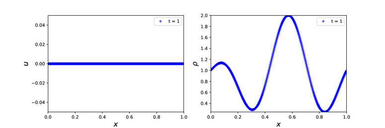
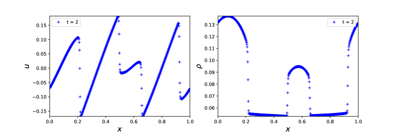
Refer to caption

Refer to caption

Refer to caption

Refer to caption

Figure 5.3: The evolution of solution u𝑢u and ρ𝜌\rho as t𝑡t increases on an expanding background.

Refer to caption

Refer to caption

Refer to caption

Figure 5.4: The evolution of solution u𝑢u and ρ𝜌\rho as t𝑡t increases on an expanding background.

Rescaling the numerical solution

We now display the rescaled solution u~~𝑢\widetilde{u} and ρ~~𝜌\widetilde{\rho} defined in (2.11); see Figure 5.5. We observe that the asymptotic solution only contains two linear pieces with two jumps, and eventually converges to a constant.
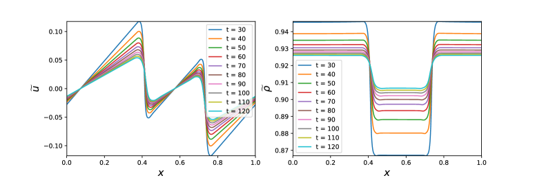
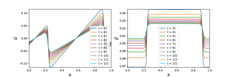
Refer to caption

Refer to caption

Refer to caption

Figure 5.5: Rescaled solution on an expanding background with k=0.5𝑘0.5k=0.5.

5.2 Flows on a spatially homogeneous background in two space dimensions

The proposed algorithm in one space dimension is applied direction by direction on a Cartesian mesh. We checked that our two-dimensional code is “consistent” with the results provided in one dimension, and in the typical test chosen above a very similar asymptotic rescaled density is recovered. We then performed genuinely two-dimensional tests, as now presented.

Similar to the one-dimensional tests we assume that a(t)=tκ𝑎𝑡superscript𝑡𝜅a(t)=t^{\kappa} and we begin with a uniform geometry b(x,y)1𝑏𝑥𝑦1b(x,y)\equiv 1, so that the source term reads

S0=κtρ(1+3ϵ2k2+(1ϵ2k2)ϵ2V2),S1=2ρκt(1+ϵ2k2)u,S2=2ρκt(1+ϵ2k2)v.formulae-sequencesubscript𝑆0𝜅𝑡𝜌13superscriptitalic-ϵ2superscript𝑘21superscriptitalic-ϵ2superscript𝑘2superscriptitalic-ϵ2superscript𝑉2formulae-sequencesubscript𝑆12𝜌𝜅𝑡1superscriptitalic-ϵ2superscript𝑘2𝑢subscript𝑆22𝜌𝜅𝑡1superscriptitalic-ϵ2superscript𝑘2𝑣\displaystyle S_{0}=-{\kappa\over t}\rho\Big{(}1+3\epsilon^{2}k^{2}+(1-\epsilon^{2}k^{2})\epsilon^{2}V^{2}\Big{)},\qquad S_{1}=-2\rho{\kappa\over t}(1+\epsilon^{2}k^{2})u,\qquad S_{2}=-2\rho{\kappa\over t}(1+\epsilon^{2}k^{2})v. (5.4)

Test 1: Symmetrical initial data.

We choose the following initial data posed at t0=1subscript𝑡01t_{0}=1 and defined in the domain [0,1]×[0,1]0101[0,1]\times[0,1]:

ρ0(x,y)=0.1+0.1e20(x0.5)220(y0.5)2,u0(x,y)=0,v0(x,y)=0.formulae-sequencesubscript𝜌0𝑥𝑦0.10.1superscript𝑒20superscript𝑥0.5220superscript𝑦0.52formulae-sequencesubscript𝑢0𝑥𝑦0subscript𝑣0𝑥𝑦0\rho_{0}(x,y)=0.1+0.1e^{-20{(x-0.5)}^{2}-20{(y-0.5)}^{2}},\qquad u_{0}(x,y)=0,\qquad v_{0}(x,y)=0. (5.5)
Refer to caption
Figure 5.6: Initial data for the spatially homogenous background in two space dimensions.

We choose this initial data (Figure 5.6) to be able to observe that the solution preserves its symmetry. In addition, in all two-dimensional tests from here, the exponent κ=2𝜅2\kappa=2, the sound speed k=0.5𝑘0.5k=0.5, CFL =0.5absent0.5=0.5, the light speed to be a unit, and the grid is [100×100]delimited-[]100100[100\times 100]. For the expanding test cases t[1,+)𝑡1t\in[1,+\infty) is chosen. Furthermore, we solve the 2-D system with a third-order strong stability preserving (SSP) Runge-Kutta solver.

In Figure 5.7, we plot the rescaled solution ρ~~𝜌\widetilde{\rho} and velocity magnitude V𝑉V at t=8𝑡8t=8, 161616, 505050, 606060, respectively. The results which are obtained by the standard HLL scheme demonstrate that the solution ρ0𝜌0\rho\to 0 and V0𝑉0V\to 0 as t𝑡t increases. The rescaled solution ρ~~𝜌\widetilde{\rho} also converges to a periodically constant state.
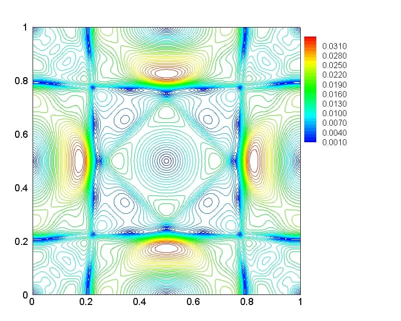
Refer to caption
Refer to caption
Refer to caption
Refer to caption
Refer to caption
Refer to caption
Refer to caption
Refer to caption
Figure 5.7: Solutions of the 2-D spatially homogeneous system in the expanding background at t=8𝑡8t=8, 161616, 505050, 606060. Right column: Rescaled solution ρ~~𝜌\widetilde{\rho}. Left column: Velocity magnitude V𝑉V.

5.3 Flows on an non-homogeneous background in one space dimension

We demonstrate here that the asymptotics of the solutions at the fine scale level is driven by the underlying background geometry.

Test 1: Stationary initial data.

We first validate the well-balanced property of the scheme, that is, it can preserve and capture smooth steady solutions of the Euler-FLRW model when a(t)1𝑎𝑡1a(t)\equiv 1. We first consider the special steady state solutions that is

u=u(x)0,ρ=ρ(x)=Cb2(x),formulae-sequence𝑢𝑢𝑥0𝜌𝜌𝑥𝐶superscript𝑏2𝑥u=u(x)\equiv 0,\qquad\rho=\rho(x)=Cb^{2}(x), (5.6)

where C𝐶C is a constant. We use different schemes to show that the modified HLL scheme is well-balanced. In this test, we choose the initial data to be

u0=0,ρ0(x)=b2(x).formulae-sequencesubscript𝑢00subscript𝜌0𝑥superscript𝑏2𝑥u_{0}=0,\qquad\rho_{0}(x)=b^{2}(x). (5.7)

at t=1𝑡1t=1, and the function b(x)𝑏𝑥b(x) to be

b(x)=1+0.01sin(2πx),𝑏𝑥10.012𝜋𝑥b(x)=1+0.01\sin(2\pi x), (5.8a)
b(x)=1+0.01(sin(6πx)+cos(2πx)),𝑏𝑥10.016𝜋𝑥2𝜋𝑥b(x)=1+0.01\big{(}\sin(6\pi x)+\cos(2\pi x)\big{)}, (5.8b)

respectively. We take N=100𝑁100N=100, ϵ=1italic-ϵ1\epsilon=1, k=0.5𝑘0.5k=0.5 and CFL=0.6𝐶𝐹𝐿0.6CFL=0.6. We plot the solution by using our proposed HLL scheme and the standard HLL scheme when t=10𝑡10t=10 (see Figure 5.8-5.9). We observe that the modified HLL scheme is able to exactly preserve the steady state solution while the standard HLL scheme cannot preserve it. Note that oscillations appear for the solution of the velocity u𝑢u.

Refer to caption
Figure 5.8: The solution on an expanding background at t=10𝑡10t=10 with (5.8a).
Refer to caption
Figure 5.9: The solution on an expanding background at t=10𝑡10t=10 with (5.8b).

Test 2: Perturbed initial data.

In this test, we choose the following initial data

u0=0,ρ0(x)={b2(x)+0.02cos(30πx),0.2x0.7,b2(x),otherwise,formulae-sequencesubscript𝑢00subscript𝜌0𝑥casessuperscript𝑏2𝑥0.0230𝜋𝑥0.2𝑥0.7superscript𝑏2𝑥otherwiseu_{0}=0,\qquad\rho_{0}(x)=\begin{cases}b^{2}(x)+0.02\cos(30\pi x),\quad&\qquad 0.2\leq x\leq 0.7,\\ b^{2}(x),&\qquad\text{otherwise},\end{cases} (5.9)

which has a perturbed density and a vanishing velocity, where b(x)𝑏𝑥b(x) is given by (5.8b). The initial data and the solution at t=10𝑡10t=10 are plotted in the Figure 5.10. We observe that even if the initial data is not a steady state solution, the solution converges to the steady state one. This shows the ability of the scheme to capture the steady state solutions.
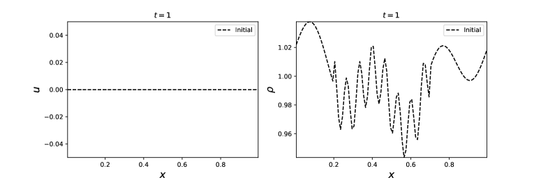
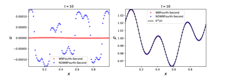
Refer to caption

Refer to caption

Figure 5.10: The solution on an expanding background.

Test 3: Perturbed initial data.

We now turn to consider the Euler model when a(t)1𝑎𝑡1a(t)\neq 1. We take here κ=2𝜅2\kappa=2, and we choose the same initial data as (5.9). We plot the solution when t=10𝑡10t=10 and t=20𝑡20t=20 (see Figure 5.11). We find that the solution ρ0𝜌0\rho\to 0 and u0𝑢0u\to 0, as t𝑡t increases.

Refer to caption

Refer to caption

Figure 5.11: Solution on an expanding background with κ=2𝜅2\kappa=2.

Rescaling the numerical solution

We now display the rescaled solution u~~𝑢\widetilde{u} and ρ~~𝜌\widetilde{\rho} defined in (2.11); see Figure 5.12. We observe that the asymptotic density converges to b2(x)superscript𝑏2𝑥b^{2}(x), while the rescaled velocity converges to 00.

Refer to caption
Figure 5.12: Rescaled solution on an expanding background at t=10𝑡10t=10.

5.4 Flows on an non-homogeneous background in two space dimensions

Similar to the one-dimensional tests, again we expect that the asymptotics of the solutions at the fine scale level is driven by the underlying background geometry which we now assume to be non-homogeneous in both spatial directions.

Test 1: Point symmetrical initial data with 𝒂(𝒕)𝟏𝒂𝒕1\boldsymbol{a(t)\equiv 1}.

We choose the following initial data posed at t0=1subscript𝑡01t_{0}=1 and defined in the domain [0,1]×[0,1]0101[0,1]\times[0,1]:

ρ0=1+0.01(sin(2πx)cos(2πx)sin(2πy)cos(2πy)),u0(x,y)=0,v0(x,y)=0,formulae-sequencesubscript𝜌010.012𝜋𝑥2𝜋𝑥2𝜋𝑦2𝜋𝑦formulae-sequencesubscript𝑢0𝑥𝑦0subscript𝑣0𝑥𝑦0\rho_{0}=1+0.01\big{(}\sin(2\pi x)\cos(2\pi x)\sin(2\pi y)\cos(2\pi y)\big{)},\qquad u_{0}(x,y)=0,\qquad v_{0}(x,y)=0, (5.10)

which is shown in Figure 5.13. Moreover, the background geometry b(x,y)𝑏𝑥𝑦b(x,y) is chosen as

b(x,y)=0.1+0.01e20(x0.5)220(y0.5)2.𝑏𝑥𝑦0.10.01superscript𝑒20superscript𝑥0.5220superscript𝑦0.52b(x,y)=0.1+0.01e^{-20{(x-0.5)}^{2}-20{(y-0.5)}^{2}}. (5.11)
Refer to caption
Figure 5.13: Initial data in two space dimensions.

The two-dimensional system is solved with the standard HLL scheme and our proposed one. In Figures 5.14 and 5.15, we plot the solution ρ𝜌\rho and velocity magnitude V𝑉V at t=8𝑡8t=8, 161616, 505050, 606060, respectively. The results of both schemes demonstrate that the solution ρCb2(x,y)𝜌𝐶superscript𝑏2𝑥𝑦\rho\to Cb^{2}(x,y) (where C𝐶C is a positive constant) as t𝑡t increases. The solutions of the well-balanced scheme converge to the steady state solution drastically faster and show significant improvements in comparison to the non-well-balanced ones. This shows the importance of using the well-balanced scheme.
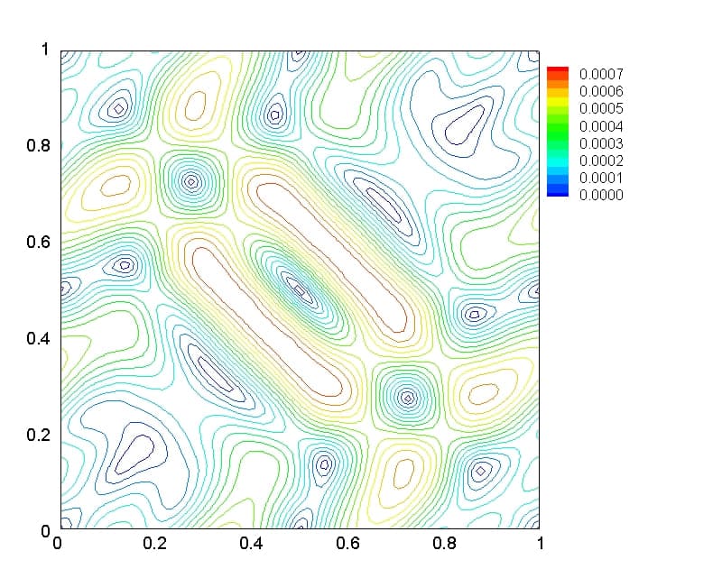
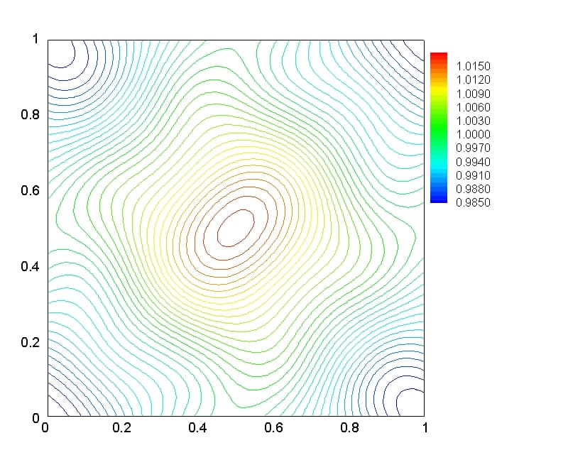
Refer to caption
Refer to caption
Refer to caption
Refer to caption
Refer to caption
Refer to caption
Refer to caption
Refer to caption
Figure 5.14: Non-well-balanced solutions of the 2-D system with a(t)1𝑎𝑡1a(t)\equiv 1 at t=8𝑡8t=8, 161616, 505050, 606060. Right column: Solution ρ𝜌\rho. Left column: Velocity magnitude V𝑉V.
Refer to caption
Refer to caption
Refer to caption
Refer to caption
Refer to caption
Refer to caption
Refer to caption
Refer to caption
Figure 5.15: Well-balanced solutions of the 2-D system with a(t)1𝑎𝑡1a(t)\equiv 1 at t=8𝑡8t=8, 161616, 505050, 606060. Right column: Solution ρ𝜌\rho. Left column: Velocity magnitude V𝑉V.

Test 2: Point symmetrical initial data in an expanding background.

In this test we demonstrate the effect of a(t)=tκ𝑎𝑡superscript𝑡𝜅a(t)=t^{\kappa} when t[1,+)𝑡1t\in[1,+\infty) over the background geometry b(x,y)𝑏𝑥𝑦b(x,y) in (5.11). We solve the two-dimensional system similar to the previous test in this section and plot the rescaled solution ρ~~𝜌\widetilde{\rho} and velocity magnitude V𝑉V at t=8𝑡8t=8, 161616, 505050, 606060, respectively. The results of both schemes demonstrate that the solution ρ0𝜌0\rho\to 0, V0𝑉0V\to 0 and the rescaled density ρ~~𝜌\widetilde{\rho} converges to Cb2(x,y)𝐶superscript𝑏2𝑥𝑦Cb^{2}(x,y) (where C𝐶C is a positive constant) as t𝑡t increases. Similar to the previous test, the rescaled solutions ρ~~𝜌\widetilde{\rho} of the well-balanced scheme converge to the steady state solution faster and show improvements in comparison to the non-well-balanced ones.
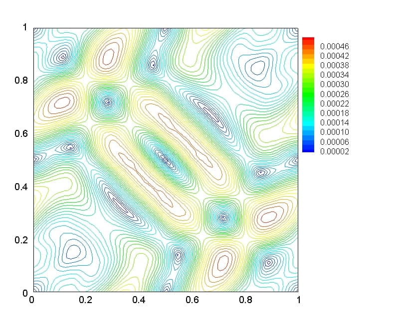
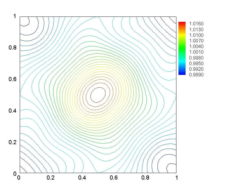
Refer to caption
Refer to caption
Refer to caption
Refer to caption
Refer to caption
Refer to caption
Refer to caption
Refer to caption
Figure 5.16: Non-well-balanced solutions of the 2-D system in an expanding background with the background geometry b(x,y)𝑏𝑥𝑦b(x,y) at t=8𝑡8t=8, 161616, 505050, 606060. Right column: Rescaled solution ρ~~𝜌\widetilde{\rho}. Left column: Velocity magnitude V𝑉V.
Refer to caption
Refer to caption
Refer to caption
Refer to caption
Refer to caption
Refer to caption
Refer to caption
Refer to caption
Figure 5.17: Well-balanced solutions of the 2-D system in an expanding background with the background geometry b(x,y)𝑏𝑥𝑦b(x,y) at t=8𝑡8t=8, 161616, 505050, 606060. Right column: Rescaled solution ρ~~𝜌\widetilde{\rho}. Left column: Velocity magnitude V𝑉V.

5.5 Conclusion for an expanding background

Based on the numerical experiments in this section, we have the following observations:

  • On a homogeneous geometry, both in one space and two space dimensions the rescaled density ρ~~𝜌\widetilde{\rho} converges to a constant, while the rescaled velocity u~~𝑢\widetilde{u} converges to zero.

  • On a non-homogeneous geometry described by a function b=b(x)𝑏𝑏𝑥b=b(x) in one space dimension and b=b(x,y)𝑏𝑏𝑥𝑦b=b(x,y) in two space dimensions, the asymptotic solution after rescaling coincides with this geometric function up to a multiplicative constant.

We thus reach the following conclusion and conjecture.

Claim 5.1 (Compressible fluid flows on a future-expanding cosmological background).

The asymptotic behavior of the solutions to the fluid model (2.1) posed on a future-expanding cosmological background is described as follows:

  • The solution (ρ,u)=(ρ,u)(t,x)𝜌𝑢𝜌𝑢𝑡𝑥(\rho,u)=(\rho,u)(t,x) (with t>0𝑡0t>0) decays to zero as t+𝑡t\to+\infty:

    limt+ρ(t,x)=0,limt+u(t,x)=0,x[0,1].formulae-sequencesubscript𝑡𝜌𝑡𝑥0formulae-sequencesubscript𝑡𝑢𝑡𝑥0𝑥01\lim_{t\to+\infty}\rho(t,x)=0,\qquad\lim_{t\to+\infty}u(t,x)=0,\qquad x\in[0,1]. (5.12)
  • Spatially homogeneous background. When the function b𝑏b is a constant, the asymptotic rescaled solution defined in (2.15) is a constant with vanishing velocity: (ρ¯,u¯)=(ρ¯,0)¯𝜌¯𝑢¯𝜌0(\overline{\rho},\overline{u})=(\overline{\rho},0). For sufficiently large times, the solution is not stationary but is approximately time-periodic. The solution propagates at the sound wave speed ±kplus-or-minus𝑘\pm k.

    • One space dimension. The rescaled density defined in (2.11) looks like two constant density states, both converging to the constant density ρ~~𝜌\widetilde{\rho}, while the velocity u~~𝑢\widetilde{u} looks like two linear parts separated by two discontinuities and both linear pieces are converging to u¯=0¯𝑢0\overline{u}=0.

    • Two space dimensions. Convergence to constant states is also observed.

  • General background. On a spatially non-homogeneous background the rescaled density ρ~~𝜌\widetilde{\rho} defined in (2.15) approaches a non-trivial limit as t+𝑡t\to+\infty of the form

    ρ¯(x)=limt+ρ~(t,x)=C1b2(x),¯𝜌𝑥subscript𝑡~𝜌𝑡𝑥subscript𝐶1superscript𝑏2𝑥\overline{\rho}(x)=\lim_{t\to+\infty}\widetilde{\rho}(t,x)=C_{1}b^{2}(x), (5.13)

    where C1>0subscript𝐶10C_{1}>0 is a constant.

6 Global dynamics on a future-contracting background

6.1 Spatially homogeneous background in one space dimension

In the future-contracting case, we now demonstrate that the density ρ+𝜌\rho\to+\infty blows up, while the velocity u𝑢u approaches the light speed value or zero.

A test with variable density data

We choose the same initial data as test 222 of the expanding background to be

u0(x)=0,ρ0(x)=1+sin(67πx)cos(72πx).formulae-sequencesubscript𝑢0𝑥0subscript𝜌0𝑥167𝜋𝑥72𝜋𝑥u_{0}(x)=0,\qquad\rho_{0}(x)=1+\sin\Big{(}{6\over 7}\pi x\Big{)}\cos\Big{(}{7\over 2}\pi x). (6.1)

We take the exponent κ=2𝜅2\kappa=2, N=500𝑁500N=500 with CFL =0.3absent0.3=0.3, and light speed to be unit. In Figure 6.1 and  6.2, we plot the evolution of the solution u𝑢u and ρ𝜌\rho as t0𝑡0t\to 0 with sound speed k=0.5𝑘0.5k=0.5. We find that ρ+𝜌\rho\to+\infty and u±1𝑢plus-or-minus1u\to\pm 1, as t0𝑡0t\to 0. We also plot the solution u𝑢u and ρ𝜌\rho when the sound speed k=0.1𝑘0.1k=0.1 in Figure 6.3, which also shows that ρ+𝜌\rho\to+\infty and u±1𝑢plus-or-minus1u\to\pm 1, as t0𝑡0t\to 0. However, u±1𝑢plus-or-minus1u\to\pm 1 when k=0.1𝑘0.1k=0.1 appears earlier than the case k=0.5𝑘0.5k=0.5. In Figure 6.4, we plot solution u𝑢u and ρ𝜌\rho with k=0.9𝑘0.9k=0.9 at t=106𝑡superscript106t=-10^{-6}. Observe that the density ρ𝜌\rho blows up, while the velocity u𝑢u closes to 00.

Rescaling the numerical solution

We now plot the rescaled solution ρ~~𝜌\widetilde{\rho} defined in (2.17) with the initial data given by (6.1) and k=0.5𝑘0.5k=0.5; see Figure 6.5. We observe that the asymptotic solution ρ~~𝜌\widetilde{\rho} approaches a bounded and stationary limit.

Refer to caption

Refer to caption

Refer to caption

Refer to caption

Figure 6.1: The evolution of solution on a contracting background with k=0.5𝑘0.5k=0.5.

Refer to caption

Refer to caption

Refer to caption

Refer to caption

Figure 6.2: The evolution of solution on a contracting background with k=0.5𝑘0.5k=0.5.
Refer to caption
Figure 6.3: The solution on a contracting background at t=104𝑡superscript104t=-10^{-4} with k=0.1𝑘0.1k=0.1.
Refer to caption
Figure 6.4: The solution on a contracting background at t=106𝑡superscript106t=-10^{-6} with k=0.9𝑘0.9k=0.9.
Refer to caption
Figure 6.5: The solution u𝑢u and rescaled solution ρ~~𝜌\widetilde{\rho} on a contracting background with k=0.5𝑘0.5k=0.5.

6.2 Flows on a spatially homogeneous background in two space dimensions

In the two-dimensional future-contracting case, we now demonstrate that the density ρ+𝜌\rho\to+\infty blows up, while the velocity magnitude V𝑉V approaches the light speed value.

Test 1: Symmetrical initial data.

We choose the initial data (5.10) posed at t0=1subscript𝑡01t_{0}=-1 and defined in the domain [0,1]×[0,1]0101[0,1]\times[0,1]. Recall that in all two-dimensional tests, the exponent κ=2𝜅2\kappa=2, the sound speed k=0.5𝑘0.5k=0.5, CFL =0.5absent0.5=0.5, the light speed to be a unit, and the grid is [100×100]delimited-[]100100[100\times 100]. In Figure 6.6, we plot the rescaled solution ρ~~𝜌\widetilde{\rho} and velocity magnitude t=0.5𝑡0.5t=-0.5, 101superscript101-10^{-1}, 103superscript103-10^{-3}, 105superscript105-10^{-5}, respectively. The results which are obtained by the standard HLL scheme demonstrate that the solution ρ+𝜌\rho\to+\infty and V1𝑉1V\to 1 as t𝑡t increases.

Refer to caption
Refer to caption
Refer to caption
Refer to caption
Refer to caption
Refer to caption
Refer to caption
Refer to caption
Figure 6.6: Solutions of the 2-D spatially homogeneous system in a contracting background at t=0.5𝑡0.5t=-0.5, 101superscript101-10^{-1}, 103superscript103-10^{-3}, 105superscript105-10^{-5}. Right column: Rescaled solution ρ~~𝜌\widetilde{\rho}. Left column: Velocity magnitude V𝑉V.

6.3 Flows on an non-homogeneous background in one space dimension

A test with variable density data

We choose the function b(x)𝑏𝑥b(x) as follows:

b(x)=1+0.01(sin(6πx)+cos(2πx)),𝑏𝑥10.016𝜋𝑥2𝜋𝑥b(x)=1+0.01\big{(}\sin(6\pi x)+\cos(2\pi x)\big{)}, (6.2)

and the initial data to be

u0=0,ρ0(x)=b2(x).formulae-sequencesubscript𝑢00subscript𝜌0𝑥superscript𝑏2𝑥u_{0}=0,\qquad\rho_{0}(x)=b^{2}(x). (6.3)

at t=1𝑡1t=-1. We take κ=2𝜅2\kappa=2. We can obtain the same result as the homogeneous case on a contracting background, that is ρ+𝜌\rho\to+\infty and u±1𝑢plus-or-minus1u\to\pm 1 or 00, as t0𝑡0t\to 0. We plot the solution u𝑢u and ρ𝜌\rho at t=107𝑡superscript107t=-10^{-7} with k=0.3𝑘0.3k=0.3, see Figure 6.7. Observe that in this case ρ+𝜌\rho\to+\infty and u±1𝑢plus-or-minus1u\to\pm 1, as t0𝑡0t\to 0. Moreover, in Figure 6.8, we plot the solution at t=107𝑡superscript107t=-10^{-7} with k=0.9𝑘0.9k=0.9. We observe that ρ+𝜌\rho\to+\infty and u0𝑢0u\to 0.

Refer to caption
Figure 6.7: The solution u𝑢u and ρ𝜌\rho on a contracting background with k=0.3𝑘0.3k=0.3.
Refer to caption
Figure 6.8: The solution u𝑢u and ρ𝜌\rho on a contracting background with k=0.9𝑘0.9k=0.9.

Rescaling the numerical solution

We now plot the rescaled solution ρ~~𝜌\widetilde{\rho} defined in (6.9). We observe that the asymptotic solution ρ~~𝜌\widetilde{\rho} approaches a bounded and stationary limit.
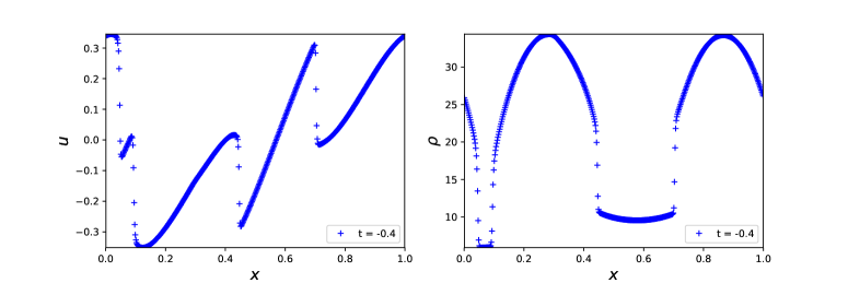
Refer to caption
Figure 6.9: The solution u𝑢u and rescaled solution ρ~~𝜌\widetilde{\rho} on a contracting background with k=0.3𝑘0.3k=0.3.

6.4 Flows on an non-homogeneous background in two space dimensions

Test 1: Point symmetrical initial data in a contracting background.

In this test we demonstrate the effect of a(t)=|t|κ𝑎𝑡superscript𝑡𝜅a(t)=|t|^{\kappa} when t[1,0)𝑡10t\in[-1,0) over the background geometry b(x,y)𝑏𝑥𝑦b(x,y) in (5.11). The two-dimensional system is solved with the standard HLL scheme and our proposed one. In Figures 6.10 and 6.11, we plot the rescaled solution ρ~~𝜌\widetilde{\rho} and velocity magnitude V𝑉V at 101superscript101-10^{-1}, 103superscript103-10^{-3}, 105superscript105-10^{-5}, 108superscript108-10^{-8}, respectively. The results of both schemes demonstrate that the solution ρ+𝜌\rho\to+\infty, and velocity magnitude V1𝑉1V\to 1 as t𝑡t increases.

Refer to caption
Refer to caption
Refer to caption
Refer to caption
Refer to caption
Refer to caption
Refer to caption
Refer to caption
Figure 6.10: Non-well-balanced solutions of the 2-D system in a contracting background with the background geometry b(x,y)𝑏𝑥𝑦b(x,y) at t=101𝑡superscript101t=-10^{-1}, 103superscript103-10^{-3}, 105superscript105-10^{-5}, 108superscript108-10^{-8}. Right column: Rescaled solution ρ~~𝜌\widetilde{\rho}. Left column: Velocity magnitude V𝑉V.
Refer to caption
Refer to caption
Refer to caption
Refer to caption
Refer to caption
Refer to caption
Refer to caption
Refer to caption
Figure 6.11: Well-balanced solutions of the 2-D system in a contracting background with the background geometry b(x,y)𝑏𝑥𝑦b(x,y) at t=101𝑡superscript101t=-10^{-1}, 103superscript103-10^{-3}, 105superscript105-10^{-5}, 108superscript108-10^{-8}. Right column: Rescaled solution ρ~~𝜌\widetilde{\rho}. Left column: Velocity magnitude V𝑉V.

6.5 Conclusion for a contracting background

Again we are able to “validate” the exponents that were derived theoretically.

Claim 6.1 (Compressible fluid flows on a future-contracting cosmological background).

The asymptotic behavior of solutions to the cosmological fluid model on a future-contracting background is as follows:

  • The density ρ=ρ(t,x)𝜌𝜌𝑡𝑥\rho=\rho(t,x) blows up as t0𝑡0t\to 0 while the velocity approaches zero or the light speed:

    limt0ρ(t,x)=+,limt0u(t,x){1,0,+1},x[0,1].formulae-sequencesubscript𝑡0𝜌𝑡𝑥formulae-sequencesubscript𝑡0𝑢𝑡𝑥101𝑥01\lim_{t\to 0}\rho(t,x)=+\infty,\qquad\lim_{t\to 0}u(t,x)\in\big{\{}-1,0,+1\big{\}},\qquad x\in[0,1]. (6.4)
  • Spatially homogeneous and non-homogeneous background. The rescaled density ρ~~𝜌\widetilde{\rho} defined in (2.17) approaches a bounded and stationary limit.
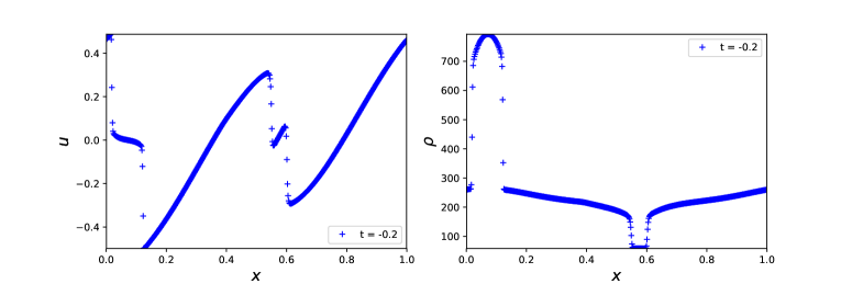
Acknowledgments. The authors were partially supported by the Innovative Training Network (ITN) ModCompShock under the grant 642768. Parts of this paper were written while the third author (PLF) was a visiting fellow at the Courant Institute of Mathematical Sciences at New York University during the Academic year 2018–2019.

References

  • [1] P. Amorim, P.G. LeFloch, and B. Okutmustur, Finite volume schemes on Lorentzian manifolds, Comm. Math. Sc. 6 (2008), 1059–1086.
  • [2] A. Baeza, S Boscarino, P. Mulet, G. Russo, and D. Zorío, Approximate Taylor methods for ODEs, Comput. & Fluids 159 (2017), 156–166.
  • [3] Y. Bakhtin and P.G. LeFloch, Ergodicity and Hopf-Lax-Oleinik formula for fluid flows evolving around a black hole under a random forcing, Stoch. Partial Differ. Equ. Anal. Comput. 6 (2018), 746–785.
  • [4] A. Beljadid and P.G. LeFloch, A central-upwind geometry-preserving method for hyperbolic conservation laws on the sphere, Commun. Appl. Math. Comput. Sci. 12 (2017), 1, 81–107.
  • [5] A. Beljadid, P.G. LeFloch, and M. Mohamadian, Late-time asymptotic behavior of solutions to hyperbolic conservation laws on the sphere, Comput. Methods Appl. Mech. Engrg. 349 (2019), 285–311.
  • [6] S. Boscarino, P.G. LeFloch, and G. Russo, High-order asymptotic-preserving methods for fully nonlinear relaxation problems, SIAM J. Sci. Comput. 36 (2014), A377–A395.
  • [7] S. Boscarino, G. Russo, and M. Semplice, High-order finite volume schemes for balance laws with stiff relaxation, Comput. & Fluids 169 (2018), 155–168.
  • [8] Y. Cao, M.A. Ghazizadeh, and P.G. LeFloch, Asymptotic structure of cosmological Burgers flows in one and two space dimensions: a numerical study, Preprint July 2019, ArXiv.
  • [9] T. Ceylan, P.G. LeFloch, and B. Okutmustur, A finite volume method for the relativistic Burgers equation on a FLRW background spacetime, Commun. Comput. Phys. 23 (2018), 500–519.
  • [10] A. Chertock, S. Cui, A. Kurganov, S.N. Özcan, and E. Tadmor, Well-balanced schemes for the Euler equations with gravitation: conservative formulation using global fluxes, J. Comput. Phys. 358 (2018), 36–52.
  • [11] J. Giesselmann, A convergence result for finite volume schemes on Riemannian manifolds, Math. Model. Numer. Anal. 43 (2009), 929–955.
  • [12] J. Giesselmann and P.G. LeFloch, Formulation and convergence of the finite volume method for conservation laws on spacetimes with boundary, Numerische Mathematik (2019).
  • [13] J. Giesselmann and T. Müller, Geometric error of finite volume schemes for conservation laws on evolving surfaces, Numer. Math. 128 (2014), 489–516.
  • [14] A. Harten, P. D. Lax, and B. V. Leer, On Upstream Differencing and Godunov-Type Schemes for Hyperbolic Conservation Laws, SIAM Rev., 25(1983), 35–61.
  • [15] P.G. LeFloch, Structure-preserving shock-capturing methods: late-time asymptotics, curved geometry, small-scale dissipation, and nonconservative products, in “Lecture Notes of the XV ’Jacques-Louis Lions’ Spanish-French school”, SEMA SIMAI Springer Series, Springer Verlag, Switzerland, 2014, pp. 179–222.
  • [16] P.G. LeFloch and H. Makhlof, A geometry-preserving finite volume method for compressible fluids on Schwarzschild spacetime, Commun. Comput. Phys. 15 (2014), 827–852.
  • [17] P.G. LeFloch, H. Makhlof, and B. Okutmustur, Relativistic Burgers equations on a curved spacetime. Derivation and finite volume approximation, SIAM J. Num. Anal. 50 (2012), 2136–2158.
  • [18] P.G. LeFloch and S. Xiang, Weakly regular fluid flows with bounded variation on the domain of outer communication of a Schwarzschild black hole spacetime, J. Math. Pures Appl. 106 (2016), 1038–1090.
  • [19] P.G. LeFloch and S. Xiang, A numerical study of the relativistic Burgers and Euler equations on a Schwarzschild black hole exterior, Commun. Appl. Math. Comput. Sci. 13 (2018), 271–301.
  • [20] D. Lengeler and T. Müller, Scalar conservation laws on constant and time-dependent Riemannian manifolds, J. Differential Equations 254 (2013), 1705–1727.
  • [21] V. Michel-Dansac, C. Berthon, S. Clain, and F. Foucher, A well-balanced scheme for the shallow-water equations with topography, Comput. Math. Appl. 72 (2016), 568–593.
  • [22] G. Russo, Central schemes for conservation laws with application to shallow water equations, S. Rionero, G. Romano Ed., Trends and Applications of Mathematics to Mechanics: STAMM 2002, Springer Verlag, Italy, 2005, pp. 225–246.
  • [23] G. Russo, High-order shock-capturing schemes for balance laws, in “Numerical solutions of partial differential equations”, Adv. Courses Math. CRM Barcelona, Birkhäuser, Basel, 2009, pp. 59–147.