Machine-Learning X-ray Absorption Spectra to Quantitative Accuracy

Abstract

Simulations of excited state properties, such as spectral functions, are often computationally expensive and therefore not suitable for high-throughput modeling. As a proof of principle, we demonstrate that graph-based neural networks can be used to predict the x-ray absorption near-edge structure spectra of molecules to quantitative accuracy. Specifically, the predicted spectra reproduce nearly all prominent peaks, with 90% of the predicted peak locations within 1 eV of the ground truth. Besides its own utility in spectral analysis and structure inference, our method can be combined with structure search algorithms to enable high-throughput spectrum sampling of the vast material configuration space, which opens up new pathways to material design and discovery.

The last decade has witnessed exploding developments in artificial intelligence, specifically deep learning applications, in many areas of our society LeCun et al. (2015), including image and speech recognition, language translation and drug discovery, just to name a few. In scientific research, deep learning methods allow researchers to establish rigorous, highly non-linear relations in high-dimensional data. This enormous potential has been demonstrated in, e.g., solid state physic and materials science Reyes and Maruyama (2019); Schmidt et al. (2019), including the prediction of molecular Rupp et al. (2012, 2015) and crystal Xie and Grossman (2018) properties, infrared Gastegger et al. (2017) and optical excitations Ye et al. (2019), phase transitions Vargas-Hernández et al. (2018) and topological ordering Rodriguez-Nieva and Scheurer (2019) in model systems, in silico materials design Sanchez-Lengeling and Aspuru-Guzik (2018) and force field development Behler and Parrinello (2007); Zhang et al. (2018).

One high-impact area of machine learning (ML) applications is predicting material properties. By leveraging large amounts of labeled data consisting of feature-target pairs, ML models, such as deep neural networks, are trained to map features to targets. The ML parameters are optimized by minimizing an objective loss criterion, and yields a locally optimal interpolating function Alpaydin (2009). Trained ML models can make accurate predictions on unknown materials almost instantaneously, giving this approach a huge advantage in terms of fidelity and efficiency in sampling the vast materials space as compared to experiment and conventional simulation methods. So far, existing ML predictions mostly focus on simple quantities, such as the total energy, fundamental band gap and forces; it remains unclear whether ML models can predict complex quantities, such as spectral functions of real materials, with high accuracy. Establishing such capability is in fact essential to both the physical understanding of fundamental processes and design of new materials. In this study, we demonstrate that ML models can predict x-ray absorption spectra of molecules with quantitative accuracy, capturing key spectral features, such as locations and intensities of prominent peaks.

X-ray absorption spectroscopy (XAS) is a robust, element-specific characterization technique widely used to probe the structural and electronic properties of materials Ankudinov et al. (2002). It measures the intensity loss of incident light through the sample caused by core electron excitations to unoccupied states Rehr and Albers (2000). In particular, the x-ray absorption near edge structure (XANES) encodes key information about the local chemical environment (LCE), e.g. the charge state, coordination number and local symmetry, of the absorbing sites Kuzmin and Chaboy (2014); Rehr and Albers (2000); Rehr et al. (2009). Consequently, XANES is a premier method for studying structural changes, charge transfer, and charge and magnetic ordering in condensed matter physics, chemistry and materials science.

To interpret XANES spectra, two classes of problems need to be addressed. In a forward problem, one simulates XANES spectra from given atomic arrangements using electronic structure theory Rehr and Albers (2000); Taillefumier et al. (2002); Prendergast and Galli (2006); De Groot and Kotani (2008); Chen et al. (2010); Vinson et al. (2011); Gulans et al. (2014). In an inverse problem, one infers key LCE characteristics from XANES spectra Timoshenko et al. (2017, 2018); Carbone et al. (2019). While the solution of the forward problem is limited by the accuracy of the theory and computational expense, it is generally more complicated to solve the inverse problem, which often suffers from a lack of information and can be ill-posed Rehr et al. (2005). Standard approaches typically rely on either empirical fingerprints from experimental references of known crystal structures or verifying hypothetical models using forward simulation Farges et al. (1997, 2001).

When using these standard approaches, major challenges arise from material complexity associated with chemical composition (e.g., alloys and doped materials) and structure (e.g., surfaces, interfaces and defects), which makes it impractical to find corresponding reference systems from experiment and incurs a high computational cost of simulating a large number of possible configurations, with hundreds or even thousands of atoms in a single unit cell. Furthermore, emerging high-throughput XANES capabilities Meirer and Weckhuysen (2018) poses new challenges for fast, even on-the-fly, solutions of the inverse problem to provide time-resolved materials characteristics for in situ and operando studies. As a result, a highly accurate, high-throughput XANES simulation method could play a crucial role in tackling both forward and inverse problems, as it provides a practical means to navigate the material space in order to unravel the structure-spectrum relationship. When combined with high-throughput structure sampling methods, ML-based XANES models can be used for the fast screening of relevant structures.

Recently, multiple efforts have been made to incorporate data science tools in x-ray spectroscopy. Exemplary studies include database infrastructure development (e.g. the computational XANES database in the Materials Project Jain et al. (2013); Ong et al. (2013, 2015); Mathew et al. (2018)), building computational spectral fingerprints Yan et al. (2019), screening local structural motifs Trejo et al. (2019), predicting LCE attributes in nano clusters Timoshenko et al. (2017) and crystals Timoshenko et al. (2018); Carbone et al. (2019) from XANES spectra using ML models. However, predicting XANES spectra directly from molecular structures using ML models has, to the best of our knowledge, not yet been attempted.

As a proof-of-concept, we show that a graph-based deep learning architecture, a message passing neural network (MPNN) Gilmer et al. (2017), can predict XANES spectra of molecules from their molecular structures to quantitative accuracy. Our training sets consist of O and N K-edge XANES spectra (simulated using the FEFF9 code Rehr et al. (2010)) of molecules in the QM9 molecular database Ramakrishnan et al. (2014), which contains $\sim$ 134k small molecules with up to nine heavy atoms (C, N, O and F) each. The structures were optimized using density functional theory with the same functional and numerical convergence criteria. This procedure, together with the atom-restriction of the QM9 database, ensures a consistent level of complexity from which a ML database can be constructed and tested. Although our model is trained on computationally inexpensive FEFF data, it is straightforward to generalize this method to XANES spectra simulated at different levels of theory.

The MPNN inputs (feature space) are derived from a subset of molecular structures in the QM9 database, henceforth referred to as the molecular structure space, $\mathcal{M}$. Two separate databases are constructed by choosing molecules containing at least one O ($\mathcal{M}_{\mathrm{O}}$, $n_{\mathrm{O}}\approx 113$k) or at least one N atom ($\mathcal{M}_{\mathrm{N}}$, $n_{\mathrm{N}}\approx 81$k) each; note that $\mathcal{M}_{\mathrm{O}}\cap\mathcal{M}_{\mathrm{N}}\neq\emptyset,$ as many molecules contain both O and N atoms. The molecular geometry and chemical properties of each molecule are mapped to a graph ($\mathcal{M}_{A}\rightarrow\mathcal{G}_{A}$, $A\in\{\mathrm{O},\mathrm{N}\}$) by associating atoms with graph nodes and bonds with graph edges. Following Ref. Gilmer et al., 2017, each $g_{i}\in\mathcal{G}_{A}$ ($i$ the index of the molecule) consists of an adjacency matrix that completely characterizes the graph connectivity, a list of atom features (absorber, atom type, donor/acceptor status, and hybridization), and a list of bond features (bond type and length). A new feature, “absorber”, is introduced to distinguish the absorbing sites from the rest of the nodes. Each graph-embedded molecule in $\mathcal{G}_{A}$ corresponds to a K-edge XANES spectrum in the spectrum or target space, $S_{A}\in\mathbb{R}^{n_{A}\times 80}$, which is the average of the site-specific spectra of all absorbing atoms, $A,$ in that molecule, spline interpolated onto a grid of 80 discretized points and scaled to a maximum intensity of 1. For each database $\mathcal{D}_{A}=(\mathcal{G}_{A},S_{A}),$ the data is partitioned into training, validation and testing splits. The latter two contain 500 data points each, with the remainder used for training. The MPNN model is optimized using the mean absolute error (MAE) loss function between the prediction $\hat{\mathbf{y}}_{i}=\mathrm{MPNN}(g_{i})$ and ground truth $\mathbf{y}_{i}\in S_{A}$ spectra. During training, the MPNN learns effective atomic properties, encoded in hidden state vectors at every atom, and passes information through bonds via learned messages. The output computed from the hidden state vectors is the XANES spectrum discretized on the energy grid as a length-80 vector. Additional details regarding the graph embedding procedure, general implementation Paszke et al. (2017); Hagberg et al. (2008); Cho et al. (2014) and MPNN operation can be found in Ref. Gilmer et al., 2017 and in the supporting information (SI) sup .

Prior to the training, we systematically examine the distribution of the data. Following common chemical intuition, the data are labeled according to the functional group that the absorbing atom belongs to. In order to efficiently deconvolute contributions from different functional groups, we only present results on molecules with a single absorbing atom each; this subset is denoted as $\mathcal{D}_{A}^{\prime}=(\mathcal{G}_{A}^{\prime},S_{A}^{\prime})\subset\mathcal{D}_{A}$, and the distribution of common functional groups in $\mathcal{D}_{A}^{\prime}$ are shown in Fig. 1, where the most abundant compounds are ethers and alcohols in $\mathcal{D}_{\mathrm{O}}^{\prime}$, and tertiary (III^∘) and secondary (II^∘) amines in $\mathcal{D}_{\mathrm{N}}^{\prime}$. From averaged spectra (bold lines) in Fig. 1, distinct spectral contrast (e.g., number of prominent peaks, peak locations and heights) can be identified between different functional groups. In fact, several trends in the FEFF spectra qualitatively agree with experiment, such as the sharp pre-edge present in ketones (black) but absent in alcohols (red) Kim et al. (2011), and the general two-peak feature of primary (I^∘) amines (blue) Plekan et al. (2007).

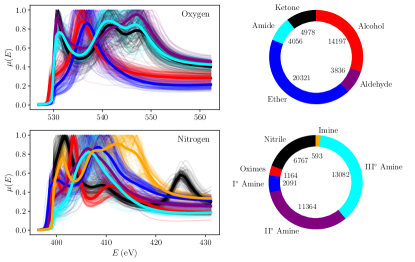
Figure 1: Left: 100 oxygen (top) and nitrogen (bottom) random sample spectra from each functional group in $S_{A}^{\prime}$; the averages over all spectra in each functional group are shown in bold. Right: the distribution of functional groups in $\mathcal{D}_{A}^{\prime}$.

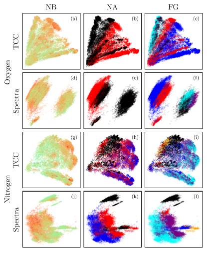
Figure 2: PCA plots for both the TCC and spectra proxies for the molecules in $\mathcal{D}^{\prime}_{A}$ labeled by NB, NA and FG. The total number of non-hydrogenic bonds (NB, top) range from 1 (violet) to 13 (red). The total number of atoms bonded to the absorbing atom (NA, center) takes on one of three values: 1, 2 or 3 (black, red and blue, respectively). The color legends for the functional group of the absorbing atom (FG, bottom) are the same as in Fig. 1.

Although XANES is known as a local probe that is sensitive to the LCE of absorbing atoms, a systematic study of the degree of such correlation on a large database has not yet been performed. To investigate this structure-spectrum correlation, we perform principal component analysis (PCA) Pearson (1901) on both the features and targets in $\mathcal{D}_{A}$, and visually examine the clustering patterns after the data in $\mathcal{D}_{A}^{\prime}$ is labeled by different chemical descriptors. To provide a baseline, we consider the total number of non-hydrogenic bonds in the molecule (NB), which is a generic, global property, supposedly having little relevance to the XANES spectra. Next we consider two LCE attributes: the total number of atoms bonded to the absorbing atom (NA) and the functional group of the absorbing atom (FG). While spectra on a discrete grid can be processed directly, molecular structures, with different number of atoms and connectivity, need to be pre-processed into a common numerical representation before clustering. Thus, the molecular fingerprint of each molecule in $\mathcal{M}_{A}$ is calculated from its SMILES code using the RDKit library RDKit, online . Then an arbitrarily large subset of $10^{4}$ molecules, $\widetilde{\mathcal{M}}_{A}\subset\mathcal{M}_{A}$, is randomly selected to construct a molecular similarity matrix of Tanimoto correlation coefficients (TCCs) Tanimoto (1958), $T_{A}\in[0,1]^{N_{A}\times 10^{4}}$, from the molecular fingerprints such that $T_{A,ij}=\mathrm{TCC}(m_{i},m_{j})$, where $m_{i}\in\mathcal{M}_{A}$ and $m_{j}\in\widetilde{\mathcal{M}}_{A}$. $\mathrm{TCC}(m_{i},m_{i})=1$ defines perfect similarity. The $T_{A}$ matrix therefore provides a uniform measure of structural similarity of every molecule in $\mathcal{M}_{A}$ to each one of the $10^{4}$ references, serving as a memory-efficient proxy to $\mathcal{M}_{A}$.

Results of the PCA dimensionality reduction are presented for both data sets and all three descriptor labels (NB, NA and FG) in Fig. 2. Specifically, after PCA is performed on unlabeled data, the data are colored in by their respective labels. While some degree of structure is manifest in NB, it is clear that the overall clustering is much inferior to both NA and FG, confirming that NB is largely irrelevant to XANES. On the other hand, both NA and FG exhibit significant clustering, with the latter, as expected, slightly more resolved; while NA can only distinguish up to 2 (3) bonds in the O (N) data sets, FGs reveal more structural details of the LCE, and encode more precise information, such as atom and bond types. For NA and FG, clustering in the TCC-space is more difficult to resolve, as it is only a course-grained description of the molecule, missing detailed information about, e.g., molecular geometry, which will be captured by the MPNN. Despite this, visual inspection reveals significant structure, such as in Fig. 2(c), where alcohols (red), ethers (blue) and amides (cyan) appear well-separated.

Spectra PCA of FG in Figs. 2(f) and 2(l) can also be directly correlated with the sample spectra in Fig. 1. For instance, the shift in the main peak position between ketones/aldehydes/amides (black/purple/cyan) and alcohols/ethers (red/blue) in $S_{\mathrm{O}}^{\prime}$ reflects the impact of a double versus a single bond on the XANES spectra. As a result, groups of these structurally different compounds are well-separated in the spectra PCA as shown in Fig. 2(f); even compounds with moderate spectral contrast, e.g., between alcohols (red) and ethers (blue), are well-separated. Similar trends are observed in $S_{\mathrm{N}}^{\prime},$ where, e.g., nitrile groups (black) show a distinct feature around 425 eV, which clearly distinguishes itself from the other FGs, and, likely because of that, one observes a distinct black cluster in Fig. 2(l).

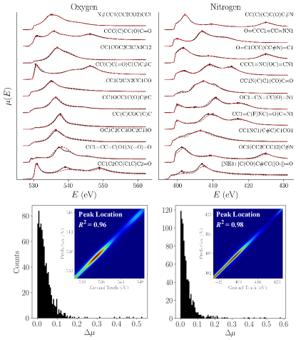
Figure 3: Performance metrics for the MPNN evaluated on the $\mathcal{D}_{A}$ testing sets. Top: waterfall plots of sample spectra (labeled by their SMILES codes) of ground truth (black) and predictions (dashed red), where prominent peaks (see text) are indicated by triangles. One randomly selected sample from every decile is sorted by MAE (first: best; last: worst). Bottom: distribution of the absolute error of predicted peak heights, $\Delta\mu$; insets show the comparison between the prediction and ground truth in peak locations.

The PCA suggests that the FG is a key descriptor of XANES. As the MPNN can fully capture the distinction of FGs through node features, edge features and the connectivity matrix, we expect that an MPNN can learn XANES spectra of molecules effectively. Randomly selected testing set results from the trained MPNN for both $\mathcal{D}_{\mathrm{O}}$ and $\mathcal{D}_{\mathrm{N}}$ are presented in Fig. 3 and ordered according to MAE, with the best decile at the top and worst decile at the bottom. It is worth noting that MPNN predictions not only reproduce the overall shape of the spectra, but, more importantly, predict peak locations and heights accurately. In the best decile, the MPNN predictions and ground truth spectra are nearly indistinguishable. Even in the worst decile, the main spectral features (e.g. three peaks between 530 and 550 eV in the oxygen K-edge and two peaks between 400 and 410 eV in nitrogen K-edge) are correctly reproduced with satisfactory relative peak heights.

As shown in Table I, the MAE of the prediction is 0.023 (0.024) for the oxygen (nitrogen) test set, which is an order of magnitude smaller than the spectral variation defined by the mean absolute deviation of the oxygen (0.131) and nitrogen (0.123) test sets. To provide an additional quantification of the model’s accuracy, we select prominent peaks, defined by those with height above half the maximum height of the spectrum and separated by a minimum 12 grid points ($\approx 6$ eV) in energy. We find that the number of prominent peaks in 95% (90%) of predicted spectra correspond with that of the ground truth for the oxygen (nitrogen) testing set. Peak locations and heights are predicted with average absolute difference of $\overline{\Delta E}=0.49$ (0.48) eV and $\overline{\Delta\mu}=0.045$ (0.041), respectively (see Table 1). The predicted peak heights display a very narrow distribution around $\Delta\mu=0$, as the total population in the tail region with $\Delta\mu>0.1$ is only 7% (see Fig. 3, bottom). As shown at the insets, the vast majority ($\sim$90%) of the predicted peak locations fall within $\pm$ 1 eV of the ground truth, with the coefficient of determination, $R^{2}\geq 0.96$. The exceptional accuracy of the MPNN model results on predicting both peak location and intensity underscores its predictive power and its ability to capture essential spectral features.

It is also important to understand the robustness of the network for practical applications; specifically, we examine how distorting or removing certain features impacts the model performance. To do so, we train separate MPNN models using “contaminated” features, where either (1) the bond length is randomized (RBL), or (2) the atom type is randomly chosen, and all other atomic features are removed (RAF). In addition, we investigate the impact of the locality in the MPNN prediction of XANES spectra of molecular systems. By default, the MPNN operates on the graph-embedding of the whole molecule, referred to as the core results. However, the significance of the FG as a sound proxy for the XANES spectra (see Fig. 2) suggests that local properties, such as the LCE, play a dominant role. Therefore, spatially truncated graphs are likely to be sufficient to predict the XANES spectra of molecules accurately. To quantify this effect, we impose different distance cutoffs ($d_{\mathrm{c}}$) from $2$ to $6$ Å around the absorbing atoms, and train separate ML models using spatially truncated graphs.

Table 1: Performance metrics based on the MAE of the spectra, $\overline{\Delta E}$ and $\overline{\Delta\mu}.$

$A$	Data	MAE	$\overline{\Delta E}$ (eV)	$\overline{\Delta\mu}$
O	Core	0.023(1)	0.52(4)	0.044(2)
	RBL	0.031(1)	0.55(3)	0.051(2)
	RAF	0.041(2)	0.63(3)	0.068(3)
	$d_{\mathrm{c}}=4\leavevmode\nobreak\ \text{\AA}$	0.023(1)	0.45(3)	0.040(2)
	$d_{\mathrm{c}}=3\leavevmode\nobreak\ \text{\AA}$	0.025(1)	0.48(3)	0.040(2)
	$d_{\mathrm{c}}=2\leavevmode\nobreak\ \text{\AA}$	0.095(4)	0.80(4)	0.179(6)
N	Core	0.024(1)	0.47(3)	0.042(2)
	RBL	0.029(1)	0.57(3)	0.049(2)
	RAF	0.045(2)	0.70(4)	0.084(3)
	$d_{\mathrm{c}}=4\leavevmode\nobreak\ \text{\AA}$	0.023(1)	0.43(3)	0.039(2)
	$d_{\mathrm{c}}=3\leavevmode\nobreak\ \text{\AA}$	0.027(2)	0.47(3)	0.046(3)
	$d_{\mathrm{c}}=2\leavevmode\nobreak\ \text{\AA}$	0.056(4)	0.66(4)	0.099(5)

Independent MPNN models were trained and tested on each database corresponding to either RBL, RAF and different $d_{\mathrm{c}}$ values. As shown in Table 1, randomizing the bond length feature does not affect the performance of MPNN, as $\overline{\Delta E}$ and $\overline{\Delta\mu}$ in RBL only worsen slightly. Atomic features have a larger impact than the bond length, as $\overline{\Delta E}$ and $\overline{\Delta\mu}$ in RAF have a sizable increase from 0.52 (0.47) to 0.63 (0.70) eV and from 0.044 (0.042) to 0.068 (0.084) in $\mathcal{D}_{\mathrm{O}}$ ($\mathcal{D}_{\mathrm{N}}$). In fact, despite the seemingly large increase, $\overline{\Delta E}$ is still well below 1 eV, i.e., falling within 1-2 grid points, resulting in only a marginal impact on its practical utility. Percentage-wise, the change in $\overline{\Delta\mu}$ is comparable to $\overline{\Delta E}$ for RAF. If we consider relative peak intensity instead of absolute peak intensity as measured by $\Delta\mu$, this difference becomes less significant.

The analysis above leads to a seemingly counter-intuitive conclusion that key XANES features can be obtained with little knowledge about the atomic features and bond length, especially if one considers the importance to know which atoms are the absorption sites. It turns out that this is not entirely surprising, since it has been shown that the distinct chemical information of atoms can be extracted by ML techniques from merely the chemical formula of the compound Zhou et al. (2018), i.e., specific atomic information can be learned through its environment. In this case, the connectivity matrix likely compensates for a lack of atom-specific information, and supplies enough knowledge about the LCE to make accurate predictions. As for the effect of the locality, we found that the results are statistically indistinguishable from the core results when $d_{\mathrm{c}}\geq 4$ Å, and breaks down at $d_{\mathrm{c}}\approx 2$ Å, indicating that the MPNN architecture requires at least the first two coordination shells to make accurate predictions.

In summary, we show that the functional group carries statistically significant information about the XANES spectra of molecules, and that by using a graph-based deep learning architecture, molecular XANES spectra can be effectively learned and predicted to quantitative accuracy. With proper generalization, this method can be used to provide a general purpose, high-throughput capability for predicting spectral information, which may not be limited to XANES, of a broad range of materials including molecules, crystals and interfaces.

M.R.C. acknowledges support from the U.S. Department of Energy through the Computational Sciences Graduate Fellowship (DOE CSGF) under grant number: DE-FG02-97ER25308. This research used resources of the Center for Functional Nanomaterials, which is a U.S. DOE Office of Science Facility, and the Scientific Data and Computing Center, a component of the Computational Science Initiative, at Brookhaven National Laboratory under Contract No. DE-SC0012704. The authors acknowledge fruitful discussions with Mark Hybertsen, Xiaohui Qu, Xiaochuan Ge and Martin Simonovsky.

References

- LeCun et al. (2015) Y. LeCun, Y. Bengio, and G. Hinton, Nature 521, 436 (2015).
- Reyes and Maruyama (2019) K. G. Reyes and B. Maruyama, MRS Bulletin 44, 530 (2019).
- Schmidt et al. (2019) J. Schmidt, M. R. Marques, S. Botti, and M. A. Marques, Npj Comput. Mater. 5, 1 (2019).
- Rupp et al. (2012) M. Rupp, A. Tkatchenko, K.-R. Müller, and O. A. von Lilienfeld, Phys. Rev. Lett. 108, 058301 (2012).
- Rupp et al. (2015) M. Rupp, R. Ramakrishnan, and O. A. Von Lilienfeld, J. Phys. Chem. Lett 6, 3309 (2015).
- Xie and Grossman (2018) T. Xie and J. C. Grossman, Phys. Rev. Lett. 120, 145301 (2018).
- Gastegger et al. (2017) M. Gastegger, J. Behler, and P. Marquetand, Chem. Sci. 8, 6924 (2017).
- Ye et al. (2019) S. Ye, W. Hu, X. Li, J. Zhang, K. Zhong, G. Zhang, Y. Luo, S. Mukamel, and J. Jiang, PNAS 116, 11612 (2019).
- Vargas-Hernández et al. (2018) R. A. Vargas-Hernández, J. Sous, M. Berciu, and R. V. Krems, Phys. Rev. Lett. 121, 255702 (2018).
- Rodriguez-Nieva and Scheurer (2019) J. F. Rodriguez-Nieva and M. S. Scheurer, Nat. Phys. 15, 790 (2019).
- Sanchez-Lengeling and Aspuru-Guzik (2018) B. Sanchez-Lengeling and A. Aspuru-Guzik, Science 361, 360 (2018).
- Behler and Parrinello (2007) J. Behler and M. Parrinello, Phys. Rev. Lett. 98, 146401 (2007).
- Zhang et al. (2018) L. Zhang, J. Han, H. Wang, R. Car, and E. Weinan, Phys. Rev. Lett. 120, 143001 (2018).
- Alpaydin (2009) E. Alpaydin, Introduction to machine learning (MIT press, 2009).
- Ankudinov et al. (2002) A. Ankudinov, J. Rehr, J. J. Low, and S. R. Bare, J. Chem. Phys. 116, 1911 (2002).
- Rehr and Albers (2000) J. J. Rehr and R. C. Albers, Rev. Mod. Phys. 72, 621 (2000).
- Kuzmin and Chaboy (2014) A. Kuzmin and J. Chaboy, IUCrJ 1, 571 (2014).
- Rehr et al. (2009) J. J. Rehr, J. J. Kas, M. P. Prange, A. P. Sorini, Y. Takimoto, and F. Vila, C R Phys 10, 548 (2009).
- Taillefumier et al. (2002) M. Taillefumier, D. Cabaret, A.-M. Flank, and F. Mauri, Phys. Rev. B 66, 195107 (2002).
- Prendergast and Galli (2006) D. Prendergast and G. Galli, Phys. Rev. Lett. 96, 215502 (2006).
- De Groot and Kotani (2008) F. De Groot and A. Kotani, Core level spectroscopy of solids (CRC press, 2008).
- Chen et al. (2010) W. Chen, X. Wu, and R. Car, Phys. Rev. Lett. 105, 017802 (2010).
- Vinson et al. (2011) J. Vinson, J. J. Rehr, J. J. Kas, and E. L. Shirley, Phys. Rev. B 83, 115106 (2011).
- Gulans et al. (2014) A. Gulans, S. Kontur, C. Meisenbichler, D. Nabok, P. Pavone, S. Rigamonti, S. Sagmeister, U. Werner, and C. Draxl, J. Phys. Condens. Matter 26, 363202 (2014).
- Timoshenko et al. (2017) J. Timoshenko, D. Lu, Y. Lin, and A. I. Frenkel, J. Phys. Chem. Lett. 8, 5091 (2017).
- Timoshenko et al. (2018) J. Timoshenko, A. Anspoks, A. Cintins, A. Kuzmin, J. Purans, and A. I. Frenkel, Phys. Rev. Lett. 120, 225502 (2018).
- Carbone et al. (2019) M. R. Carbone, S. Yoo, M. Topsakal, and D. Lu, Phys. Rev. Materials 3, 033604 (2019).
- Rehr et al. (2005) J. Rehr, J. Kozdon, J. Kas, H. Krappe, and H. Rossner, J. Synchrotron Radiat. 12, 70 (2005).
- Farges et al. (1997) F. Farges, G. E. Brown, J. Rehr, et al., Phys. Rev. B 56, 1809 (1997).
- Farges et al. (2001) F. Farges, G. E. Brown Jr, P.-E. Petit, and M. Munoz, Geochim. Cosmochim. Acta 65, 1665 (2001).
- Meirer and Weckhuysen (2018) F. Meirer and B. M. Weckhuysen, Nat. Rev. Mater. 3, 324 (2018).
- Jain et al. (2013) A. Jain, S. P. Ong, G. Hautier, W. Chen, W. D. Richards, S. Dacek, S. Cholia, D. Gunter, D. Skinner, G. Ceder, and K. A. Persson, APL Mater. 1, 011002 (2013).
- Ong et al. (2013) S. P. Ong, W. D. Richards, A. Jain, G. Hautier, M. Kocher, S. Cholia, D. Gunter, V. L. Chevrier, K. A. Persson, and G. Ceder, Comput. Mater. Sci. 68, 314 (2013).
- Ong et al. (2015) S. P. Ong, S. Cholia, A. Jain, M. Brafman, D. Gunter, G. Ceder, and K. A. Persson, Comput. Mater. Sci. 97, 209 (2015).
- Mathew et al. (2018) K. Mathew, C. Zheng, D. Winston, C. Chen, A. Dozier, J. J. Rehr, S. P. Ong, and K. A. Persson, Sci. Data 5, 180151 (2018).
- Yan et al. (2019) D. Yan, M. Topsakal, S. Selcuk, J. L. Lyons, W. Zhang, Q. Wu, I. Waluyo, E. Stavitski, K. Attenkofer, S. Yoo, et al., Nano Lett. (2019).
- Trejo et al. (2019) O. Trejo, A. L. Dadlani, F. De La Paz, S. Acharya, R. Kravec, D. Nordlund, R. Sarangi, F. B. Prinz, J. Torgersen, and N. P. Dasgupta, Chem. Mater. (2019).
- Gilmer et al. (2017) J. Gilmer, S. S. Schoenholz, P. F. Riley, O. Vinyals, and G. E. Dahl, in Proceedings of the 34th International Conference on Machine Learning-Volume 70 (JMLR. org, 2017) pp. 1263–1272.
- Rehr et al. (2010) J. Rehr, J. Kas, F. Vila, M. Prange, and K. Jorissen, Phys. Chem. Chem. Phys. 12, 5503 (2010).
- Ramakrishnan et al. (2014) R. Ramakrishnan, P. O. Dral, M. Rupp, and O. A. von Lilienfeld, Sci. Data 1 (2014).
- Paszke et al. (2017) A. Paszke, S. Gross, S. Chintala, G. Chanan, E. Yang, Z. DeVito, Z. Lin, A. Desmaison, L. Antiga, and A. Lerer, in NIPS Autodiff Workshop (2017).
- Hagberg et al. (2008) A. Hagberg, P. Swart, and D. S Chult, Exploring network structure, dynamics, and function using NetworkX, Tech. Rep. (Los Alamos National Lab.(LANL), Los Alamos, NM (United States), 2008).
- Cho et al. (2014) K. Cho, B. Van Merriënboer, D. Bahdanau, and Y. Bengio, arXiv preprint arXiv:1409.1259 (2014).
- (44) “Supplemental Material (url will be inserted by publisher) includes the technical details of the MPNN.” .
- Kim et al. (2011) K. Kim, P. Zhu, N. Li, X. Ma, and Y. Chen, Carbon 49, 1745 (2011).
- Plekan et al. (2007) O. Plekan, V. Feyer, R. Richter, M. Coreno, M. De Simone, K. Prince, and V. Carravetta, J Electron Spectrosc 155, 47 (2007).
- Pearson (1901) K. Pearson, Philos. Mag. 2, 559 (1901).
- (48) RDKit, online, “RDKit: Open-source cheminformatics,” http://www.rdkit.org.
- Tanimoto (1958) T. T. Tanimoto, Tech. Rep., IBM Internal Report (1958).
- Zhou et al. (2018) Q. Zhou, P. Tang, S. Liu, J. Pan, Q. Yan, and S.-C. Zhang, Proc. Natl. Acad. Sci. 115, E6411 (2018).