Boundary action and profile of effective bosonic strings

Abstract:

The mean-square width of the energy profile of the bosonic string is calculated considering two boundary terms in the effective LW action. The perturbative expansion of the Lorentz-invariant boundary terms at the second and the fourth order in the effective action is taken around the free Nambu-Goto string. The calculation is presented for open strings with Dirichlet boundary condition on a cylinder.

1 Introduction

The confinement of quarks is an essential property of quantum chromodynamics (QCD) and strong interactions. Despite the tremendous research efforts to provide mechanisms of quark confinement based dynamical gluonic degrees of freedom of the QCD, there is no compelling analytical construction for the phenomenon of confinement starting from basic principles.

The confinement property can be probed directly in the Monte-Carlo evaluations of QCD path integrals. The computer simulations of the infinitely heavy quark-antiquark ($Q\bar{Q}$) bound state revealed the linear rise property [1, 2, 3, 4] of confining potential.

It is understood from this observation that the linear rise of the potential at long separation between two static $Q\bar{Q}$ is due to the gluonic field [5, 6, 7, 8, 9, 10, 11, 12, 13, 14] which appears to be condensed into a stringlike flux tube. The formation of stringlike flux tube in between the color sources provides a prospective technique for the confinement of quarks. In this model, the nonperturbave properties of the QCD flux-tubes are expected to conform with that of an effective bosonic strings with fixed edges in the long string limit.

The string formation manifests in many strongly correlated systems  [15, 16, 17, 18] and can be described after roughening transition by an effective string action. The effective string action is a low energy effective field theory [19] which is obtained by integrating out the degrees of freedom of Yang-Mills (YM) vacuum in the presence of two static quarks. This string description supplies a tool to predict a set of infrared (IR) observables  [71, 72, 73, 74, 75, 72, 76, 77, 78, 79, 80] which can be confronted with the outcomes from the numerical lattice data.

The Lüscher term is an essential  [20, 21] prediction associated with the string’s quantum fluctuations at zero temperature. This Casimir energy is a detectable subleading correction to the linearly rising $Q\bar{Q}$ potential [22, 23] which is universal to any gauge group. The Lüscher term has been detected in the numerical simulations of either Wilson [24] or Polyakov loop correlation function representing $Q\bar{Q}$ static pair [25, 26, 27, 28, 29, 30, 31, 32]. The Y-string [33, 35, 34] binding the three quark  [37, 38] in baryonic configurations produces a counterpart Lüscher-like term which have been detected in abelian lattice gauge system [35].

Not only the static potential but also the energy chart of the QCD vacuum in the presence of the confined color sources [36] and its characteristic broadening is a fundamental source to probe the physics of the confinement from first principles. Many lattice simulations of many gauge groups have unambiguously verified [39, 40, 41, 42, 43, 44, 26, 45, 46, 47, 48] the predicted logarithmic broadening [49] of the confining strings and the linear behavior [50] near the confinement point and large distances.

Nevertheless, the analysis of string’s fine structure in the lattice numerical data for the broadening profile revealed substantial deviations [51, 52, 53] from the free-string Nambu-Goto (NG) model in the intermediate distance region at high temperatures. The excited spectrum [47] and finite temperature string tension  [54, 55, 56] obtained from the partition function of the leading-order Gaussian formulation of NG string action show a similar disagreement with the numerical data  [26, 56, 52, 114, 58, 59, 57] for distance scales less than $1.0$ fm.

The higher-order corrections are terms of the asymptotic expansion in the inverse powers of color source separation distance $1/R$ associated with the interaction terms of growing dimensions. The next to leading correction terms of the NG action [61, 62, 63] have been subjected to numerical investigations [64, 65, 66, 42, 67, 48, 68, 69, 70] to ascertain the relevance order by order to the discrepancy from the numerical data in each gauge model. In fact, there is no proof neither evidence that all orders [22, 23] of the power expansion are universal.

The effective bosonic string theory serves as a functional tool in many QCD processes  [71, 72, 73, 74, 75, 72, 76, 77, 78, 79, 80]. The precise study of the strings effects suggests considering other features beyond the free NG action [81], in particular, possible stiffness properties [82, 83] and boundary term corrections [84, 85, 86, 87].

The Lorentz invariant boundary corrections [86] to the static $Q\bar{Q}$ potential have shown viable in both the Wilson and the Polyakov-loop correlators cases [84, 85, 114, 58, 59]. The boundary corrections to the static quark potential provide an explanation to the deviations lately discovered among predictions of the effective string and numerical outcomes [24].

The broadening profile of the energy field should receive similar corrections from the Lorentz invariant boundary terms in the action. However, the contributions of the boundary action to the width profile have neither been theoretically calculated nor confronted with the numerical lattice data. These corrections are hoped to account to many features of the fine structure of the profile of QCD flux-tube in IR region. In particular it could account for the well known deviations at relatively short distances at low temperatures, or larger distances for the excited spectrum of the flux-tubes [85, 89] and at high temperatures [88, 114, 58, 59].

The goal of the present paper is to analytically estimate the mean-square width resulting from the boundary terms in Lüscher-Weisz (LW) effective string action. The calculations are laid out for open string with Dirichlet boundary condition on a cylinder. This could be compatible with the energy fields set up by a static mesonic configurations. We consider the perturbative expansion of two boundary terms at the order of fourth and six derivative and evaluate the modification to the mean-square width around the free NG string.

2 Effective action of bosonic strings

Long stringlike objects are not uncommon in field theory. The magnetic vortices in superconductors [93, 94], cosmic strings [96, 97] admits an effective string descriptions as well. The property of linearly rising potential suggests that the YM vacuum admits the presence of an object such as a quite thin long string, which is responsible for transmitting the strongly interacting forces among the quarks. The conjecture is in consistency [90] with the dual superconductive [91, 92, 93, 94, 95, 28] QCD vacuum and the formation of a vortex line dual to the Abrikosov by the virtue of the dual Meissner effect.

The effective field theory description holds at distance scales larger than the scale intrinsic thickness of the string [98, 99]. The classical long string solution entails, however, the breaking of the $(D-2)$ transverse translational symmetry leading to the associated transverse oscillations of massless Goldston modes [100, 101].

The Lagrangian of the low energy effective field theory [31] may be constructed from all the terms respecting the imposed symmetries on the system [102]. To constrain the effective action of the confining string Polchinski-Strominger (PS) [103] introduced a conformal gauge on the worldsheet. Within this formalism, the action is constraint by requiring the effective field theory to be ghost free which fixes the central charge to be D=26 [103, 80]. The conformal theory is manifestly Lorentz-invariant and the leading term of PS action coincides with the 4-derivative term of the NG string [80]. However, it appears that this technique is untraceable especially at higher orders.

However, Lüscher, Symanzik and Weisz [104, 105] suggested that the effective action of the string connecting a stable pair of $Q\bar{Q}$ in D-dimensional confining the theory of Yang-Mills can be constructed by the leading term of NG, free, action. In fact, the LW effective action admits all terms which preserves Lorentz and transnational-invariance [106] and is expressed in physical degrees of freedom. The effective action respects Lorentz symmetry through nonlinear realization of this symmetry [108, 109, 110] since the worldsheet gauge diffeomorphism is fixed to static/physical gauge. The nonlinearly-realized Lorentz symmetry constrains the coefficients of the higher-order terms in the action which is found to coincide with that of the NG action up to $\mathcal{O}(1/R^{3})$ in the long string expansion.

As mentioned above, an effective string action can be constructed from the derivative expansion of collective string co-ordinates fulfilling Poincare and parity invariance. The operators of the Goldstone fields in the action are perturbations around the classical solution and necessarily are space-time derivatives to preserve the translation invariance. In addition, the terms in the action that are proportional to the equation of motion or its derivatives do not contribute in perturbation theory and can be absorbed by field redefinition. These fluctuations $X^{i}$ (in $D-2$ space-time dimensions) are massless and in the static/physical gauge $X^{1}=\zeta_{1},X^{4}=\zeta_{2}$ are restricted to transverse directions ${\cal C}$. With this prescription, the LW effective action  [104, 105] up to 4-derivative term come into the form

$$\begin{split}S_{LW}[\mathbf{X}]&=S_{cl}+\dfrac{\sigma}{2}\int d^{2}\zeta\Big{(}\dfrac{\partial\mathbf{X}}{\partial\zeta_{\alpha}}\cdot\dfrac{\partial\mathbf{X}}{\partial\zeta_{\alpha}}\Big{)}+\sigma\int d^{2}\zeta\Bigg{[}c_{2}\Big{(}\dfrac{\partial\mathbf{X}}{\partial\zeta_{\alpha}}\cdot\dfrac{\partial\mathbf{X}}{\partial\zeta_{\alpha}}\Big{)}^{2}+c_{3}\Big{(}\dfrac{\partial\mathbf{X}}{\partial\zeta_{\alpha}}\cdot\dfrac{\partial\mathbf{X}}{\partial\zeta_{\beta}}\Big{)}^{2}\Bigg{]}\\ &+\gamma\int d\zeta^{2}\sqrt{g}\mathcal{R}+\alpha\int d\zeta^{2}\sqrt{g}\mathcal{K}^{2}+...+S_{b},\end{split}$$ (1)

where we have considered the Euclidean signature. The vector $X^{\mu}(\zeta^{0},\zeta^{1})$ maps the area $C\subset\mathbb{R}^{2}$ into $\mathbb{R}^{4}$, the geometrical invariants $\mathcal{R}$ and $\mathcal{K}$ define Ricii-scalar and the extrinsic curvature  [82, 83] of the corresponding configuration of world sheet, respectively. The term $S_{cl}$ characterizes the classical term, on the quantum level the Weyl invariance of the action is broken in four dimensions; however, the anomaly is known to vanish at large distances [90].

Cylindrical boundary conditions explicitly break translation invariance of the classical solution, this would entail the emergence of terms other than that in bulk of the effective action. The boundary action $S_{b}$ is a surface term located at the boundaries $\zeta^{1}=0$ and $\zeta^{1}=R$. This ought to signifies the interplay of the effective string with either the Polyakov loops on the fixed ends of the string or Wilson’s loop which we will discuss in detail in the next section.

The couplings $c_{1}$, $c_{2}$ in LW action Eq. (1) are the parameters of effective low-energy theory. For the next-to-leading order terms in $D$ dimension the open-closed duality [47] imposes further constraint on these kinematically-dependent couplings to

$$(D-2)c_{2}+c_{3}=\left(\dfrac{D-4}{2\sigma}\right).$$ (2)

Moreover, it has been shown [63] through a nonlinear Lorentz-transform in terms of the string collective variables $X_{i}$  [111] that the action is invariant under $SO(1,D-1)$. By this symmetry the couplings Eq.(2) of the four derivative term in the LW action Eq.(1) are not arbitrary and are fixed in any dimension $D$ by

$$c_{2}+c_{3}=\dfrac{-1}{8\sigma}.$$ (3)

Condition (3) implies that all the terms with only first derivatives in the effective string action Eq.(1) coincide with the corresponding one in Polyakov-Kleinert action in the derivative expansion.

$$S=-\int d^{2}\zeta\sqrt{-{\rm{det}}g_{\alpha\beta}}\left(\sigma+\frac{1}{\alpha}(\mathcal{K}_{\alpha\beta})^{2}\right),$$ (4)

where $g$ is the two-dimensional induced metric on the world sheet embedded in the background $\mathbb{R}^{4}$, $\alpha$ is the rigidity parameter.

3 Lorentz-invariant boundary terms

The Lorentz symmetry which is a basic feature of YM theory dictates constraints [110, 109, 62, 112] over the arbitrary coefficients appearing on the effective action expansion. The string field operators of the action should be built such that these crucial symmetries are preserved. In this paper we theoretically calculate the width profile of effective open strings with boundary action made up of Lorentzian invariants.

First we naively set out the possible form of each order in the Lagrangian density and then guided by requirement of fulfilling Lorentz symmetry the relevant terms are deduced at each coupling. We consider the case of Dirichlet boundary conditions $X^{i}=0$ at both ends, pure $\zeta^{0}$-derivatives vanish on the boundary ($\partial_{0}^{n}X=0$). A Generic boundary action is defined as

$$S_{b}=\int d\zeta^{0}\left[\mathcal{L}_{1}+\mathcal{L}_{2}+\mathcal{L}_{3}+\mathcal{L}_{4}+...\right],$$ (5)

with the Lagrangian density $\mathcal{L}_{i}$ for each effective low-energy coupling $b_{i}$. The worldsheet coordinates have dimensions of length, a bulk term has the same order as a boundary term with one less derivative. The operator has to have an odd number $n$ of spatial derivatives $\partial^{n}_{1}X$ so that it has non-vanishing value.

At the lowest order, the general allowed form is schematically proportional to $\partial^{2}{\mathbf{X}}^{2}$ and the only possible term [105] in the Lagrangian is therefore

$$\mathcal{L}_{1}=b_{1}{\partial_{1}\mathbf{X}}\cdot{\partial_{1}\mathbf{X}}.$$ (6)

Consistency with the open-closed string duality [47] implies a vanishing value of the first boundary coupling $b_{1}=0$, as we will discuss below the Lorentz invariance requirement implies the vanishing of $b_{1}$ as well.

The leading order corrections due to second boundary terms with the coupling $b_{2}$ appears at the four derivative term in the bulk. On the boundary the general term is of the form $\partial^{3}{\mathbf{X}}^{2}$, apart from a term proportional to the equation of motion there is naively only one possible term

$$\mathcal{L}_{2}=b_{2}{\partial_{0}\partial_{1}\mathbf{X}}\cdot{\partial_{0}\partial_{1}\mathbf{X}}~{},$$ (7)

The effective action preserves the transverse rotation symmetry $SO(d-2)$, the complete $SO(1,d-1)$ Lorentz invariance is spontaneously broken by the classical solution around which we expand, but the expanded action still respects this symmetry non-linearly the rotations in $(i,j)$ plane generates

$$\delta_{ij}X^{i}=\epsilon X^{j}.$$ (8)

In order to keep the gauge-fixing $\sigma^{1}=X^{1}$ we must make a diffeomorphism

$$\begin{split}\delta_{12}\zeta^{1}=&\epsilon X^{2}(\zeta^{1}),\\ \delta_{12}\zeta^{0}=&0,\end{split}$$ (9)

that is, Eq.(8) generates rotation which should be followed by reparamterization Eq. (9) to put the system again in the static gauge. The full nonlinear Lorentz transformation is then

$$\delta^{\alpha i}X^{j}=-\epsilon\left(\delta^{ij}\zeta^{\alpha}+X^{i}\partial^{\alpha}X^{j}\right),$$ (10)

where $\epsilon$ is an infinitesimal parameter of boosts and rotations. For each boundary action

$$S_{b_{i}}=\int_{\partial\Sigma}d\zeta^{0}\mathcal{L}_{i}.$$ (11)

The application of the infinitesimal transformation Eq.(10) and requiring the action $S_{b_{i}}$ to vanish we obtain constraints on the values of the couplings; or realize higher-order derivatives in the choice of the action of a given coupling.

The nonlinear transformation Eq. (10) of the Lagrangian densities Eq. (7) and Eq. (15) generates higher-order terms at the same scaling [110, 63] which should still acquire the same couplings. The scaling of a given term defines the order of the generated terms when applying the transformation. That is, the transform Eq. (10) of $\partial^{m}X^{n}$ generates terms with the same value of the difference $m-n$. The Lorentz transform of the Lagrangian density Eq. (7) we have two basis terms $(\partial_{1}\partial_{0}X)^{2}$ and $\partial_{1}\partial_{0}\mathbf{X}\cdot\partial_{1}\mathbf{X}$

$$\mathcal{L}_{2}=b_{2}\sum_{k=0}^{\infty}\big{[}\alpha_{k}\partial_{1}\partial_{0}\mathbf{X}\cdot\partial_{1}\partial_{0}\mathbf{X}(\partial_{1}\mathbf{X}\cdot\partial\mathbf{X})^{k}+\beta_{k+1}(\partial_{1}\partial_{0}\mathbf{X}\cdot\partial_{1}\mathbf{X})^{2}(\partial_{1}\mathbf{X}\cdot\partial_{1}\mathbf{X})^{k}\big{]}.$$ (12)

The invariance of (7) leads to recursion relations when solved Ref.[63] give rise to

$$\mathcal{L}_{2}=b_{2}\left(\dfrac{\partial_{0}\partial_{1}\mathbf{X}\cdot\partial_{0}\partial_{1}\mathbf{X}}{1+\partial_{1}\mathbf{X}\cdot\partial_{1}\mathbf{X}}-\dfrac{(\partial_{0}\partial_{1}\mathbf{X}\cdot\partial_{1}\mathbf{X})^{2}}{(1+\partial_{1}\mathbf{X}\cdot\partial_{1}\mathbf{X})^{2}}\right).$$ (13)

However, for the third order we find then

$$\mathcal{L}_{3}=b_{3}\left(\partial_{1}\mathbf{X}\cdot\partial_{1}\mathbf{X}\right)^{2}.$$ (14)

The variation of the boundary actions at first and third orders with infinitesimal nonlinear Lorentz transform Eq.(10) of the Lagrangian densities Eq.(6) and Eq.(14) entails vanishing value for $b_{1}=0$ and $b_{3}=0$.

The next order, $\mathcal{L}_{4}$, the general effective Lagrangian on the boundary is

$$\mathcal{L}_{4}=b_{4}\partial_{0}^{2}\partial_{1}\mathbf{X}\cdot\partial_{0}^{2}\partial_{1}\mathbf{X}.$$ (15)

The first two terms derived in Ref.[63] are given by

$$\mathcal{L}_{4}=b_{4}\Bigg{(}\frac{\partial_{0}^{2}\partial_{1}\mathbf{X}\cdot\partial_{0}^{2}\partial_{1}\mathbf{X}}{1+\partial_{1}\mathbf{X}\cdot\partial_{1}\mathbf{X}}-\dfrac{(\partial_{0}^{2}\partial_{1}\mathbf{X}\cdot\partial_{1}\mathbf{X})^{2}+4(\partial_{0}^{2}\partial_{1}\mathbf{X}\cdot\partial_{0}\partial_{1}\mathbf{X})(\partial_{0}\partial_{1}\mathbf{X})}{(1+\partial_{1}\mathbf{X}\cdot\partial_{1}\mathbf{X})^{2}}+...\Bigg{)}.$$ (16)

The action at the boundaries drive infinitesimal diffusion from generic source/sink into the energy density along the QCD flux tube. This causes perturbation from the free NG string behavior which is expected to evidently affect the static potential  [24, 84, 85, 114, 58, 59] and the profile near the color sources, short separation distances as well as high temperatures [114, 58, 59, 88] and excited spectrum [53]. In the next section, we shall lay out the perturbative expansion of the boundary action and estimate the subsequent augmentation/lessening of mean-square width of the effective string in $D$ dimension at any temperature.

4 The boundary terms contribution to the energy width

Let us consider the free NG action around which the perturbative expansion is taken

$$S_{\ell o}[\mathbf{X}]=S_{cl}+\dfrac{\sigma}{2}\int d\zeta^{1}\int d\zeta^{0}\Big{(}\dfrac{\partial\mathbf{X}}{\partial\zeta^{\alpha}}\cdot\dfrac{\partial\mathbf{X}}{\partial\zeta^{\alpha}}\Big{)},$$ (17)

The next-to-leading NG term combined with the expansion of the surface term on the boundary

$$\begin{split}S^{\rm{Pert}}[\mathbf{X}]&=S_{n\ell o}+S_{b},\\ &=\left(S_{n\ell o}+S_{b_{2}}+S_{b_{4}}+..\right)+....,\end{split}$$ (18)

defines the perturbation from the effective LW action Eq. (1) with higher-order geometrical terms left out .

The mean-square width of the string is defined as the second moment of the field with respect to the center of mass of the string $X_{0}$ and is given by

$$W^{2}(\zeta)=\dfrac{\int DX(\mathbf{X}(\zeta^{1},\zeta^{0})-\mathbf{X_{0}})^{2}e^{-S[\mathbf{X}]}}{\int D\mathbf{X}e^{-S[\mathbf{X}]}},$$ (19)

Expanding around the free-string action Eq. (17) the squared width of the string  [113] is given by

$$\begin{split}W^{2}(\zeta^{1})&=W_{\ell o}^{2}(\zeta^{1})-\langle\mathbf{X}^{2}(\zeta^{0},\zeta^{1})S^{\rm{Pert}}\rangle_{0}+2\gamma\langle\partial_{\alpha}\mathbf{X}^{2}(\zeta^{0},\zeta^{1})\rangle_{0}+\gamma^{2}\langle\partial_{\alpha}^{2}\mathbf{X}^{2}(\zeta^{0},\zeta^{1})\rangle_{0}\\ &-\dfrac{\gamma^{2}}{L_{T}R}\int d\zeta^{0}~{}d\zeta^{1}~{}d\zeta^{0^{\prime}}~{}d\zeta^{1^{\prime}}\langle\partial_{\alpha}^{2}\mathbf{X}(\zeta^{0},\zeta^{1})\cdot\partial_{\alpha^{\prime}}^{2}\mathbf{X}(\zeta^{0^{\prime}},\zeta^{1^{\prime}})\rangle_{0}.\end{split}$$ (20)

where the vacuum expectation value $\langle...\rangle_{0}$ is with respect to the free-string partition function, $\gamma$ is an effective low energy parameter and $L_{T}$ is the length of compactified time direction for cylindrical boundary condition.

Substituting Eq. (18) in the low-energy parameter expansion Eq. (20) the mean-square width

$$\begin{split}W^{2}(R,L_{T})=&\left\langle(\mathbf{X}^{2}(\zeta^{1},\zeta^{0})S_{\ell o})\right\rangle-\left\langle(\mathbf{X}^{2}(\zeta^{1},\zeta^{0})S_{n\ell o}+\mathbf{X}^{2}(\zeta^{1},\zeta^{0})S_{b_{2}}+\mathbf{X}^{2}(\zeta^{1},\zeta^{0})S_{b_{4}}+...)\right\rangle,\\ =&W^{2}_{\ell o}(R,L_{T})+W_{n\ell o}^{2}+W^{2}_{b}(R,L_{T})+...\\ \end{split}$$

with the contribution of the boundary action

$$W^{2}_{b}(R,L_{T})=W^{2}_{b_{2}}(R,L_{T})+W^{2}_{b_{4}}(R,L_{T}),$$

and the mean square width of the free string

$$W^{2}_{\ell o}(R,L_{T})=\dfrac{\int DX(\mathbf{X}(\zeta^{1},\zeta^{0}))^{2}e^{-S_{\ell o}[\mathbf{X}]}}{\int DXe^{-S_{\ell o}[\mathbf{X}]}}.$$ (21)

The Green-function defines the two-point free propagator

$$G\left(\zeta^{0},\zeta^{1};\zeta^{0^{\prime}},\zeta^{1^{\prime}}\right)=\langle\mathbf{X}(\zeta^{0},\zeta^{1})\cdot\mathbf{X}(\zeta^{0^{\prime}},\zeta^{1^{\prime}})\rangle,$$ (22)

which is the solution of Laplace equation on a cylindrical sheet [113] of surface area $RL_{T}$ and is given in spectral form  [113] by

$$G(\mathbf{\zeta;\zeta^{\prime}})=\frac{1}{\pi\sigma}\sum_{n=1}^{\infty}\frac{1}{n\left(1-q^{n}\right)}\sin\left(\frac{\pi n\zeta^{1}}{R}\right)\sin\left(\frac{\pi n\zeta^{1^{\prime}}}{R}\right)\left(q^{n}e^{\frac{\pi n(\zeta^{0}-\zeta^{0^{\prime}})}{R}}+e^{-\frac{\pi n(\zeta^{0}-\zeta^{0^{\prime}})}{R}}\right),$$ (23)

where $q=e^{\frac{-\pi L_{T}}{R}}$ is the complementary nome. The Dirichlet boundary condition corresponding to fixed displacement vector at the ends $\zeta^{1}=0$ and $\zeta^{1}=R$ and periodic boundary condition in time $\zeta^{0}$ with period $L_{T}$  [113] are encoded in the above propagator.

The expectation value  [39, 115, 68] of the mean-square width corresponds to the Green-function correlator of the free bosonic string theory in two dimensions

$$W^{2}_{{\ell o}}(\zeta_{1},\tau)=\frac{D-2}{2\pi\sigma_{0}}\log\left(\frac{R}{R_{0}(\zeta_{1})}\right)+\frac{D-2}{2\pi\sigma_{0}}\log\left|\,\dfrac{\vartheta_{2}(\pi\,\zeta_{1}/R;\tau)}{\vartheta_{1}^{\prime}(0;\tau)}\right|,$$ (24)

where $\theta$ are Jacobi elliptic functions

$$\theta_{1}(\zeta;\tau)=2\sum_{n=0}^{\infty} (-1)^{n}q_{1}^{n(n+1)+\frac{1}{4}}\sin((2n+1)\,\zeta),$$

$$\theta_{2}(\zeta;\tau)=2\sum_{n=0}^{\infty} q_{1}^{n(n+1)+\frac{1}{4}}\cos((2n+1)\zeta),$$ (25)

with $q_{1}=e^{\frac{i\pi}{2}\tau}$, and $R^{2}_{0}$ is the UV cutoff which has been generalized to be dependent on distances from the sources. The above formula Eq. (24) can be pinned down through the standard relations between the elliptic Jacobi and Dedkind $\eta$ functions to either of the equivalent forms derived in Refs. [113, 114, 58, 59].

The NLO term from the low energy parameter expansion Eq.(4) to the width of NG string have been worked out in detail in Ref.[113], the width due to the self-interaction is modified by

$$\begin{split}W^{2}_{n\ell o}=&\dfrac{(D-2)\pi}{12\sigma^{2}R^{2}}\Big{\{}\tau\Big{(}q\frac{d}{dq}-\frac{D-2}{12}E_{2}(\tau)\Big{)}\left[E_{2}(2\tau)-E_{2}(\tau)\right]-\frac{D-2}{8\pi}E_{2}(\tau)\Big{\}}\\ &+\frac{\pi}{12\sigma R^{2}}\left[E_{2}(\tau)-4E_{2}(2\tau)\right]\left(W_{lo}^{2}-\frac{D-2}{4\pi\sigma}\right).\end{split}$$ (26)

In the following we evaluate the correction to the mean-square width of the free string with Lorentz invariant boundary action at these two orders. We consider the expectation value of the quadratic field excitation up to the leading order term in the boundary action (35).

The perturbative expansion of the boundary action $S_{b_{2}}$ corresponding to the Lagrangian density Eq.(7) is given by

$$S_{b_{2}}=b_{2}\int_{\partial\Sigma}d\zeta^{0}\left(\partial_{0}\partial_{1}\mathbf{X}\cdot\partial_{0}\partial_{1}\mathbf{X}-\left(\partial_{0}\partial_{1}\mathbf{X}\cdot\partial_{0}\partial_{1}\mathbf{X}\right)\left(\partial_{1}\mathbf{X}\cdot\partial_{1}\mathbf{X}\right)+...\right).$$ (27)

The generic form of the Wick-contracted term representing the perturbative contribution of the boundary term to the expectation value is

$$\langle X^{2}S_{b2}\rangle=b_{2}(\langle(\mathbf{X}\cdot\mathbf{X})\partial_{0}^{2}\partial_{1}^{2}(\mathbf{X}\cdot\mathbf{X})\rangle+\langle\partial_{0}\partial_{1}(\mathbf{X}\cdot\mathbf{X})\partial_{0}\partial_{1}(\mathbf{X}\cdot\mathbf{X})\rangle).$$ (28)

Upon point-splitting the expectation value in terms of Green propagators the mean-square width becomes

$$W^{2}_{b_{2}}=-(D-2)b_{2}\int_{\partial\Sigma}d\zeta^{0^{\prime}}\lim_{\begin{subarray}{c}\zeta^{\prime}\to\zeta\end{subarray}}\big{[}\partial_{0}\partial_{1^{\prime}}G(\mathbf{\zeta;\zeta^{\prime}})\partial_{0^{\prime}}\partial_{1}G(\mathbf{\zeta^{\prime};\zeta})+G(\mathbf{\zeta;\zeta^{\prime}})\partial_{0}\partial_{1}\partial_{0^{\prime}}\partial_{1^{\prime}}G(\mathbf{\zeta^{\prime};\zeta})\big{]}.$$ (29)

the above two terms define the sum of the expectation values

$$W^{2}_{b_{2}}=-\left(W^{2}_{1,b_{2}}+W^{2}_{2,b_{2}}\right).$$ (30)

Substituting the free Green propagator Eq.(23) in the above expectation value. We perform the integrals over $\zeta^{0}$ after evaluating the derivatives and rewriting the resulting summations in closed form.

The evaluation of the two correlators Eq.(30) involve cumbersome manipulations, we present the detailed calculus in Appendix(B). The $\zeta$-function regularization of the divergent sums is performed on each expectation value appearing in the limits, $\epsilon,\epsilon^{\prime}\to 0$. The mean-square width $W^{2}_{b_{2}}$ turn out to be

$$\begin{split}W^{2}_{b_{2}}(R,L_{T})=&\frac{-\pi^{3}b_{2}(D-2)}{16R^{5}\sigma^{2}}\Bigg{(}\frac{1}{3}E_{2}(2i\tau)+2\frac{\vartheta_{1}^{\prime}}{\vartheta_{1}}\left(\frac{i\pi}{2}\tau,q\right)^{(1)}-\frac{91}{6}\Bigg{)}.\end{split}$$ (31)

In Wilson loops [116, 24, 63] operators the boundary action survives over both the spatial and temporal extends, the boundary action is given by

$$S_{b_{2}}=b_{2}\int_{\partial\Sigma_{t}}d\zeta^{0}\left(\partial_{0}\partial_{1}\mathbf{X}\cdot\partial_{0}\partial_{1}\mathbf{X}\right)+b_{2}\int_{\partial\Sigma_{s}}d\zeta^{1}\left(\partial_{0}\partial_{1}\mathbf{X}\cdot\partial_{0}\partial_{1}\mathbf{X}\right),$$ (32)

this surface term lives on the boundary $\partial\Sigma$ which in the action Eq. (32) is conveniently chosen as a rectangle-shaped Wilson’s loop circumfering the spatial-temporal area of $R\times L$, the curves $\partial\Sigma_{t}$ and $\partial\Sigma_{s}$ stands for temporal and spatial parts of the loop, respectively.

The direct calculation of the expectation value of the $\langle S_{b}\rangle$ entails contributions from both the temporal and spatial parts to the static quark potential [24]. As a consequence of the symmetry of the propagator Eq. (23), these two corrections give similar formulas [24]; however, with the role between the source separation, $R$, and temporal extent, $L$, exchanged. Moreover, the contribution from the temporal path is formally equivalent [24] to that of two Polyakov loop with the identification of the temporal height of the Wilson’s loop $L$ instead of the cylindrical time extend $L_{T}\to L$.

The generalization of the expectation value of the width due to two Polyakov loops Eq.(34) to that due to the Wilson’s loop is accordingly evaluated as the expectation value of

$$\mathcal{W}^{2}_{b_{2}}=\langle X^{2}S_{b_{2}}\rangle_{\partial\Sigma_{t}}+\langle X^{2}S_{b_{2}}\rangle_{\partial\Sigma_{s}},$$ (33)

for the boundary action given by Eq.(32). The spatial part of this expectation value is an integral of the diffused energy of the string along the spatial path the infinitesimal-time interval of either the creation/annihilation of the static quark-antiquark pair. As the mean-square width can be deduced to have the form

$$\mathcal{W}^{2}_{\square,b_{2}}(\tau;b_{2})=W^{2}_{b_{2}}\left(R,L_{T}\right)+W^{2}_{b_{2}}\left(L_{T},R\right)$$ (34)

where $L$ is the temporal extend of Wilson loop.

The next Lorentz invariant non-vanishing Lagrangian density is Eq.(15) corresponding to the coupling $b_{4}$, we consider the leading term in the expansion of boundary action

$$S_{b_{4}}=b_{4}\int_{\partial\Sigma}d\zeta^{0}\left(\partial_{0}\partial_{1}\mathbf{X}.\partial_{0}\partial_{1}\mathbf{X}-\left(\partial_{0}\partial_{1}\mathbf{X}.\partial_{0}\partial_{1}\mathbf{X}\right)\left(\partial_{1}\mathbf{X}.\partial_{1}\mathbf{X}\right)+...\right).$$ (35)

The Wick-contraction of the operator $X^{2}$ with the leading term yields the expectation value

$$\langle\mathbf{X}^{2}S_{b4}\rangle=b_{4}\langle(\mathbf{X}\cdot\mathbf{X})\partial_{0}^{2}\partial_{1}^{2}(\mathbf{X}\cdot\mathbf{X})\rangle+\langle\partial_{0}\partial_{1}(\mathbf{X}\cdot\mathbf{X})\partial_{0}\partial_{1}(\mathbf{X}\cdot\mathbf{X})\rangle.$$ (36)

The expectation value Eq.(36) in terms of Green propagators after point-splitting become

$$W^{2}_{b_{4}}=-(D-2)b_{4}\int_{\partial\Sigma}d\zeta^{0^{\prime}}\lim_{\begin{subarray}{c}\zeta^{\prime}\to\zeta\end{subarray}}\left(\partial_{0}\partial_{1^{\prime}}G(\mathbf{\zeta;\zeta^{\prime}})\partial_{0^{\prime}}\partial_{1}G(\mathbf{\zeta^{\prime};\zeta})+G(\mathbf{\zeta;\zeta^{\prime}})\partial_{0}\partial_{1}\partial_{0^{\prime}}\partial_{1^{\prime}}G(\mathbf{\zeta^{\prime};\zeta})\right).$$ (37)

Similarly, substituting the free propagator Eq.(23) in the above expectation value and integrating over $\zeta^{0}$, see Appendix(C) for details. The expectation value of the fourth-order boundary term in the action

$$W^{2}_{b_{4}}=-\left(W^{2}_{1,b_{4}}+W^{2}_{2,b_{4}}\right),$$ (38)

which turn up as,

$$W^{2}_{b_{4}}(R,L_{T})=\frac{\pi^{5}(D-2)b_{4}}{32R^{7}\sigma^{2}}\Bigg{(}\frac{2}{15}E_{4}\left(2i\tau\right)+\frac{1}{3}E_{2}\left(2i\tau\right)-\frac{7}{60}-2\frac{\vartheta_{1}^{\prime}}{\vartheta_{1}}\left(\frac{i\pi}{2}\tau,q\right)^{(1)}-32\Bigg{)},$$ (39)

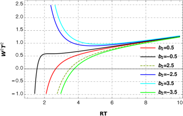
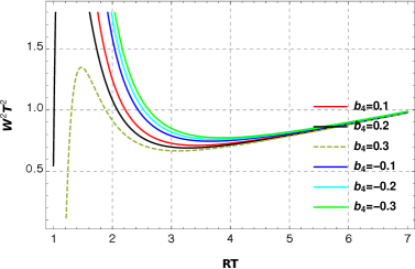
Figure 1: The plot compares the mean-square width of the effective string bounded by two Polyakov-loops at the depicted values of the boundary coupling $b_{2}$ and $b_{4}$ in the middle plane.The contribution of the boundary action to the width profile $W^{2}(R/2)=W^{2}_{\rm{NG_{(\ell o)}}}(R/2)+W^{2}_{b}$ of the leading order NG string; however, at temperature scale $L_{T}a^{-1}=6$.

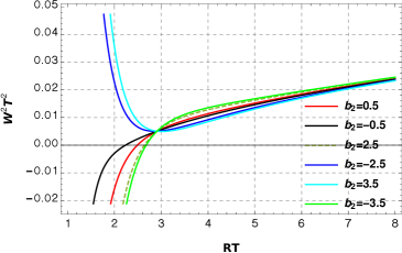
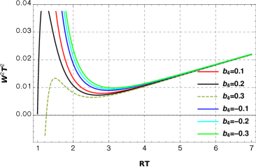
Figure 2: The plot compares the mean-square width of the effective string bounded by two Polyakov-loops at the depicted values of the boundary coupling $b_{2}$ and $b_{4}$ in the middle plane.The contribution of the boundary action to the width profile $W^{2}(R/2)=W^{2}_{\rm{NG_{(n\ell o)}}}(R/2)+W^{2}_{b}$ of the next to leading order NG string at zero temperature.

On the otherhand, the corresponding boundary corrections of the width of Wilson loop at coupling $b_{4}$ can be deduced following up the same line of reasoning leading to Eq.(34). The next-to-leading boundary correction for Wilson loop of rectangular area $L\times R$ is, accordingly, given by

$$\begin{split}\mathcal{W}^{2}_{\square;b_{4}}(\tau;b_{4})=W^{2}_{b_{4}}(R,L_{T})+W^{2}_{b_{4}}\left(L_{T};R\right)\end{split}$$ (40)

The leading non-vanishing boundary corrections to the flux-tube width Eq.(31) indicate an inverse decrease with the third power of the length scale $R$. This suggests effects that are more noticeable near the intermediate and short string length scale. In Fig.2 the mean-square width $W^{2}$, of the free NG string Eq.(24) and self-interacting NG string Eq.(26) togather with the boundary corrections Eq.(31), are plotted at the middle plane versus the string length such that

$$W^{2}(R/2)=W^{2}_{\rm{\ell o}}(R/2)+W^{2}_{n\ell o}+W^{2}_{b_{2}}+W_{b_{4}}^{2},$$ (41)

On Fig.1 we compare modifications in the width profile which were received from the depicted positive/negative values of the coupling parameter $b_{2}$ and $b_{4}$ in Eq.(31) and Eq.(39).

The boundary term $S_{b_{2}}$ in the effective string action may increase or decrease the mean-square width of NG string depending on whether positive or negative values of the coupling parameter $b_{2}$ are considered. However, the resultant effects on the width is a compromise between the value of the two couplings $b_{2}$ and $b_{4}$ and the corresponding signs.

As expected from the dimensional considerations the remarkable effects of the corrections occur over the intermediate and short string length scale. The diffusion of the interaction from the sources at the boundaries along the string is more stringent for relatively short string length. For the values of $b_{4}$ considered in Fig.1 the $S_{b_{4}}$ boundary term in the action appears to dominate and can in principle fine tune the width at shorter distances.

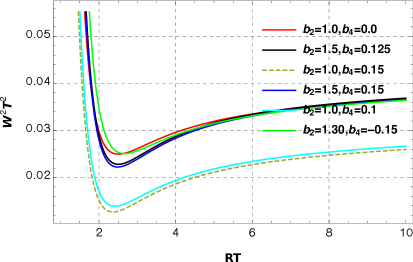
Figure 3: Compares the profile of the effective string at next to leading order in NG action for the depicted values of the couplings $b_{2}$ and $b_{4}$ ($W^{2}=W^{2}_{\rm{n\ell o}}(R/2)+\mathcal{W}^{2}_{b_{2}}+\mathcal{W}_{b_{4}}^{2}$) of Wilson loop of area $R\times L$ with $L{a}^{-1}=4$ time slices at zero temperature $T=0$.

The comparison of the mean-square width of the free NG string with the corresponding self-interacting string for a fixed value of the coupling $b_{2}$ and $b_{4}$ reveals subtle dilution of the boundary action effects if considered with the associated self-interaction of NG string. This suggests diffusion attenuated to some extend with the viscose medium driven by the self-interacting string field.

In Fig.3(a) we plot the width of the effective string versus the source separation and zero temperature in the middle plane of the string. The plot compares the width profile of the self-interacting string -Eq.(24) and Eq.(26)- setup by Wilson loop

$$W^{2}(R/2)=W^{2}_{\rm{n\ell o}}(R/2)+\mathcal{W}^{2}_{\square,b_{2}}+\mathcal{W}_{\square,b_{4}}^{2},$$ (42)

with $\mathcal{W}^{2}_{\square,b_{2}}$ and $\mathcal{W}^{2}_{\square,b_{4}}$ are given by Eq.(34) and Eq.(40), respectively. The first term in Eq.(42) signifies the zero temperature logarithmic prodening of the effective string. A similar plot in Fig.3(b) illustrates; however, the perturbative mean-square width with the decrease of the temperature Eq.(42). The plot shows the convergence of the solutions in the limit of infinite temporal $L_{T}\to\infty$ extend.

The corrections provided by the boundary action to static $Q\bar{Q}$ potential seem to explain to some extend the deviations appearing when constructing the static mesonic states with Polyakov loop correlators [89]. The $Q\bar{Q}$ potential is well described by the up to surprisingly small distances as $R=0.3$ fm using the boundary action at temperature near the end of QCD Plateau $T/T_{c}=0.8$ fm. At a higher temperature, the inclusion of the boundary corrections up to the fourth order $b_{4}$ together with string rigidity has been found  [88] to be viable in providing good fits for distances as small as $R=0.5$ fm.

The lattice simulations of the energy-density profile is a more challenging quantity to measure compared to the $Q\bar{Q}$ potential. The exponentially decaying field corelators involve the field strength tensor leading  [51, 52, 53, 35] to a substantial numerical effort  [68, 113, 114, 58, 59, 88] to attain a good enough precision.

The boundary corrections to the mean-square width of the flux-tube dictated by Eq.(29) could be relevant to fine deviations such as those famed to occur on intermediate source separation scale. The detection of these subtleties is, of course, subject to the continuous improvement in the resolution of the lattice data and computational power. Nevertheless, one would expect an impact of these terms if to carry out the numerical investigations with the Wilson loop operators [39].

5 Summary and Conclusion

In this work, the width of the energy profile of string bounded by two Polyakov loops is derived as a function of the temperature in any dimension $D$. We have considered LW string with two Lorentz invariant subleading boundary terms in the effective action.

The mean-square width have been estimated as a low energy perturbative expansion around the free string action. The width is derived for open strings with Dirichlet boundary condition on cylinder. We have implemented the technique of the $\zeta$-function regularization to the quadratic operators in the corresponding expectation values of the mean-square width of the string.

The main findings in the present paper is the boundary correction to mean-square width of the flux-tube constructed by two Polyakov loops which given by Eq.(31) at the coupling order $b_{2}$ of the Lagrangian density at the boundaries. The corrections induced by the next Lorentz invariant term at coupling $b_{4}$ have been estimated as well and are given in Eq.(38). The expectation values of two Polyakov loops can be directly generalized to Wilson’s loop, where the boundary action survives in both the spatial and temporal extents, are given by Eq.(34) and Eq.(40) at coupling $b_{2}$ and $b_{4}$, respectively.

The fine structure of the mean-square width dictated by Eq.(31) and Eq.(38) indicates effects at the fifth order in the inverse length scale $1/R^{5}$. This could be relevant to QCD strings at relatively small quark separations but where the long effective string theory still holds.

It would be interesting to investigate the width profile taking into account the boundary action in the numerical simulation of Abelian and non-Abelian  [117, 118, 119, 120, 121, 122, 84, 67, 28] gauge groups. In particular, the generalization of the calculation presented in this paper to Wilson loops [118, 116, 24, 63, 126] operators where more impact of the boundaries is expected. The excited meson [123, 124, 125] or baryonic configurations [123, 127, 128, 129, 37, 38, 130, 131] are very relevant system to discuss the boundary corrections.

Appendix A Appendix: Functions and Identities

Zeta Regularization
In the following, we quote the partition some of basic properties of the zeta-regularized products [132]. Let us consider the convergence index which is the least integer $h$ such that the series for $Z[h+1]$ converges absolutely.

• Partition Property.
  Let $\{\varphi^{1}\}_{k}$ and $\{\varphi^{2}\}_{k}$ be $\bm{\zeta}$- and let regularizable sequences $\{\varphi\}_{k}=\{\varphi^{1}\}_{k}\cup\{\varphi^{2}\}_{k}$ disjoint union then

  $$\prod_{k}\varphi_{k}=\prod_{k}\{\varphi^{1}\}_{k}\prod_{k}\{\varphi^{2}\}_{k}$$ (43)

• Splitting Property.
  If $\{\varphi_{k}\}$ is zeta-regularizable and $\prod_{k}a_{k}$ is convergent absolutely then

  $$\prod_{k}a_{k}\varphi_{k}=\prod_{k}a_{k}\prod_{k}\varphi_{k}$$ (44)

Identity I

The Jacobi elliptic $\vartheta_{1}$ function [133] of the first kind is defined as

$$\vartheta_{1}(z,q) = 2\sqrt[4]{q}\sin(z)\prod_{k=1}^{\infty}\left(1-q^{2k}\right)\left(1-2q^{2k}\cos(2z)+q^{4k}\right),$$ (45)

$$\vartheta_{2}(z,q) = 2\sqrt[4]{q}\cos(z)\prod_{k=1}^{\infty}\left(1-q^{2k}\right)\left(1+2q^{2k}\cos(2z)+q^{4k}\right),$$ (46)

$$\vartheta_{3}(z,q) = \prod_{k=1}^{\infty}\left(1-q^{2k}\right)\left(1+2q^{2k-1}\cos(2z)+q^{4k-2}\right),$$ (47)

$$\vartheta_{4}(z,q) = \prod_{k=1}^{\infty}\left(1-q^{2k}\right)\left(1-2q^{2k-1}\cos(2z)+q^{4k-2}\right),$$ (48)

(49)

with the nome defined as $q=e^{i\pi\tau}\land\Im(\tau)>0$.

Identity II

The logarithmic derivatives of $\vartheta_{1}(z,q)$ can be expressed as a series sum of hyperbolic functions as

$$\sum_{k=-\infty}^{\infty}\coth(\pi k\lambda+z)=\frac{\vartheta_{1}^{\prime}\left(iz,e^{-\pi\lambda}\right)}{\vartheta_{1}\left(iz,e^{-\pi\lambda}\right)}.$$ (50)

Identity III

The series expansion of the derivative of $\frac{\vartheta_{1}^{\prime}}{\vartheta_{1}}(z,q)$

$$\sum_{k=-\infty}^{\infty}\text{csch}(\pi k\lambda+z)^{2}=\frac{i\vartheta_{1}^{\prime\prime}\left(iz,e^{-\pi\lambda}\right)}{\vartheta_{1}\left(iz,e^{-\pi\lambda}\right)}-\frac{\vartheta_{1}^{\prime}\left(iz,e^{-\pi\lambda}\right)^{2}}{\vartheta_{1}\left(iz,e^{-\pi\lambda}\right)^{2}}.$$ (51)

Identity IV

The modular $\pi\tau$ increase to the argument of $\vartheta_{1}$ function has the property [133]

$$\vartheta_{1}(\pi\tau+z,q)=-\frac{e^{-2iz}}{q}\vartheta_{1}(z,q).$$ (52)

For $m\in\mathbb{Z}$

$$\vartheta_{1}(z+m\pi\tau,q)=(-1)^{m}q^{-m}\vartheta_{1}(z,q)\exp(-i(\pi(m-1)m\tau+2mz)).\\$$ (53)

The modular increase of the logarithmic derivative can be deduced from properties of $\vartheta_{1}$ function, for $m=1$ we obtain

$$\frac{\vartheta_{1}^{\prime}(z\pm{\pi}\tau,q)}{\vartheta_{1}(z\pm{\pi}\tau,q)}=\frac{\vartheta_{1}^{\prime}(z,q)}{\vartheta_{1}(z,q)}\pm{2}i,$$ (54)

and $m=-1,+1$

$$\frac{\vartheta_{1}^{\prime\prime}(z\pm{\pi}\tau,q)}{\vartheta_{1}(z\pm{\pi}\tau,q)}=\frac{\vartheta^{\prime\prime}\left(z,q\right)}{\vartheta_{1}\left(z,q\right)}\mp{4}\frac{i\vartheta_{1}^{\prime}\left(z,q\right)}{\vartheta_{1}\left(z,q\right)}-4.$$ (55)

Identity V

The logarithm of $\vartheta_{1}(z,q)$ is given by

$$\log(\vartheta_{1}(z,q))=4\sum_{k=1}^{\infty}\frac{q^{2k}\sin^{2}(kz)}{k\left(1-q^{2k}\right)}+\log(\vartheta_{1}^{\prime}(0,q))+\log(\sin(z)).$$ (56)

The first derivative of the logarithm of $\vartheta_{1}(z,q)$

$$\frac{\vartheta_{1}^{\prime}(z,q)}{\vartheta_{1}(z,q)}=4\sum_{k=1}^{\infty}\frac{q^{2k}\sin(2kz)}{1-q^{2k}}+\cot(z).$$ (57)

Identity VI

The derivative of the Eq.(56) at $z=0$ blow up owing to the involved two terms. The divergent sum is regularized with $\mathbf{\zeta}$ function. The divergence of the second term is eliminated by expanding $cot(z)$ around $x=0$ such that

$$\begin{split}\cot(z)&=-\frac{i\left(e^{-iz}+e^{iz}\right)}{e^{-iz}-e^{iz}},\\ &=\frac{x+\frac{1}{x}}{\frac{1}{x}-x},\\ &=1+2x^{2}+2x^{4}+2x^{6}+2x^{8}+2x^{10}+...,\\ &=-i(1+2\zeta(0)),\\ &=0,\end{split}$$ (58)

since $\zeta(0)=-\dfrac{1}{2}$.

Similarly, the derivative of the Eq.(57) at $z=0$ produce divergence of $\csc^{2}(z)$. Let $x=e^{-iz}$ and expanding $\csc(z)^{2}$ around $x=0$

$$\begin{split}\csc(x)^{2}&=x^{2}+2x^{4}+3x^{6}+4x^{8}+5x^{10}+...,\\ \lim_{x\to 1}\csc(x)^{2}&=(1+2+3+4+...)=\sum_{k=1}^{\infty}k,\\ &=\mathbf{\zeta}(1),\\ &=-1/12.\end{split}$$ (59)

The second derivative of the Eq.(57) at $z=0$ produce divergence of $2\cot(x)\csc(x)^{2}$. Expanding around $x=0$

$$\begin{split}\cot(x)\csc(x)^{2}&=8i(x^{2}+4x^{4}+9x^{6}+16x^{8}+25x^{10}+...),\\ \lim_{x\to 1}\cot(x)\csc(x)^{2}&=8i(1+4+9+16+...)=\sum_{k=1}^{\infty}k^{2},\\ &=\mathbf{\zeta}(2),\\ &=0.\end{split}$$ (60)

Expanding the third derivative of the Eq.(57) produces $-2\csc^{4}(x)-4\cot^{2}(x)\csc^{2}(x)$

$$\begin{split}-2\csc^{4}(x)-4\cot^{2}(x)\csc^{2}(x)&=-16(x^{2}+8x^{4}+27x^{6}+64x^{8}+125x^{10}+...),\\ \lim_{x\to 1}\left(-2\csc^{4}(x)-4\cot^{2}(x)\csc^{2}(x)\right)&=-16(1+8+27+64+...)\\ &=-16\sum_{k=1}^{\infty}k^{3},\\ &=\mathbf{\zeta}(3),\\ &=\dfrac{-16}{120}.\end{split}$$ (61)

The fourth derivative follow similarly,

$$\begin{split}8\cot^{3}(z)\csc^{2}(z)+16\cot(z)\csc^{4}(z)&=-32i(x^{2}+16x^{4}+81x^{6}+256x^{8}+625X^{10}+...),\\ \lim_{x\to 1}\left(8\cot^{3}(z)\csc^{2}(z)+16\cot(z)\csc^{4}(z)\right)&=-32i(1+16+81+265+...)\\ &=-16\sum_{k=1}^{\infty}k^{4},\\ &=\mathbf{\zeta}(4),\\ &=0.\end{split}$$ (62)

Identity VII

The Eisenstein series is defined as

$$E_{2k}(\tau)=1+(-1)^{k}\frac{4k}{B_{k}}\sum_{n=1}^{\infty}\frac{n^{2k-1}q^{n}}{1-q^{n}},$$ (63)

where $B_{k}$ are Bernoulli numbers which are given in terms of Riemann zeta functions as

$$\mathbf{\zeta}(2k)=\frac{B_{k}(2\pi)^{k}}{2k!},~{}~{}~{}~{}~{}~{}~{}~{}~{}\mathbf{\zeta}(1-2k)=(-1)^{k}\frac{B_{k}}{2k}.$$ (64)

for even and odd numbers respectively.
In particular $E_{2}$ and $E_{4}$ are given by

$$E_{2}(\tau)=1-24\sum_{n=1}^{\infty}\frac{nq^{n}}{1-q^{n}}.\\$$

and

$$E_{4}(\tau)=1+240\sum_{n=1}^{\infty}\frac{n^{3}q^{n}}{1-q^{n}}.\\$$

Identity VIII

The following products appear in Eq.(102) as a result of the algebraic manipulations involved in the sums and are related to elliptic $\vartheta_{4}$ through the identities given below

$$\begin{split}\mathcal{P}_{1}&=\prod_{k=1}^{\infty}\left(e^{-\frac{\pi kL}{R}-\frac{2\pi L}{R}+\frac{2\pi t}{R}}-1\right)\left(1-e^{-\frac{\pi kL}{R}+\frac{\pi L}{R}-\frac{2\pi t}{R}}\right),\\ &=\prod_{k=1}^{\infty}(e^{-\frac{\pi kL}{R}+\frac{\pi L}{R}-\frac{2\pi t}{R}}+e^{-\frac{\pi kL}{R}-\frac{2\pi L}{R}+\frac{2\pi t}{R}}-e^{-\frac{2\pi kL}{R}-\frac{\pi L}{R}}-1),\\ &=\prod_{k=1}^{\infty}(-1-e^{-\frac{\pi kL}{R}-\frac{\pi L}{2R}}+e^{-\frac{1}{2}\left(\frac{2\pi kL}{R}+\frac{\pi L}{R}\right)}\left(e^{\frac{\pi kL}{R}+\frac{2\pi L}{R}-\frac{2\pi t}{R}}+e^{\frac{\pi kL}{R}-\frac{\pi L}{R}+\frac{2\pi t}{R}}\right)/e^{-\frac{1}{2}\left(\frac{2\pi kL}{R}+\frac{\pi L}{R}\right)})\\ &=\prod_{k=1}^{\infty}(-1-e^{-\frac{\pi kL}{R}-\frac{\pi L}{2R}}+e^{\frac{1}{2}\left(\frac{2\pi kL}{R}+\frac{\pi L}{R}\right)}\cosh\left(\frac{3\pi L}{2R}-\frac{\pi t}{R}\right)),\\ &=\frac{\vartheta_{4}\left(\frac{i(3L\pi)}{4R}-\frac{i(\pi t)}{R},e^{-\frac{L\pi}{2R}}\right)}{G_{1}};~{}~{}\text{with}~{}~{}G_{1}=\prod_{k=1}^{\infty}\left(1-e^{-\frac{\pi kL}{R}}\right).\\ \end{split}$$ (65)

Identity IX

The modular increase of the argument of the elliptic $\vartheta_{4}$ is given by the identity

$$\vartheta_{4}(z+im\log(q),q)=(-1)^{m}q^{-m^{2}}e^{2imz}\vartheta_{4}(z,q),$$ (66)

$\forall m\in\mathcal{Z}$

Identity X

The elliptic $\vartheta_{4}(z,q)$ are related to $\vartheta_{1}(z,q)$ functions through the relation

$$\vartheta_{1}(z,q)=i\sqrt[4]{q}e^{-iz}\vartheta_{4}\left(z+\frac{\pi\tau}{2},q\right),$$ (67)

Identity XI

The logarithmic derivative of $\vartheta_{4}^{\prime}(z,q)$ in series form is given by

$$\frac{\vartheta_{4}^{\prime}(z,q)}{\vartheta_{4}(z,q)}=4\sum_{n=1}^{\infty}\frac{q^{n}\sin(2nz)}{1-q^{2n}}.$$ (68)

Identity XII

Let $\varphi=\frac{\pi(L_{T}-4\zeta^{0})}{4R}$ and

$$\begin{split}(z_{1}=x+iy;z_{2}=-x+iy),\\ x=\frac{\pi\zeta^{0}}{R};y=-\frac{\pi\zeta^{1}}{R},\end{split}$$ (69)

the sum of the series

$$4\sum_{m=1}^{\infty}\frac{e^{-\frac{\pi L_{T}m}{2R}}\left(\sinh\left(2m\varphi-\frac{2i\pi m\zeta^{1}}{R}\right)\right)}{1-e^{-\frac{\pi L_{T}m}{R}}}=\frac{\vartheta_{4}^{\prime}}{\vartheta_{4}}(z_{1}+\frac{\pi\tau}{2}),$$ (70)

can be expressed in the form of Jacobi elliptic function $\vartheta_{4}(\tau)$ (Eq.(66)-Eq(68). In addition, the following invariant subtraction follows from Eq.(68)

$$\frac{\vartheta_{4}^{\prime}}{\vartheta_{4}}(z_{2}+\frac{\pi\tau}{2})-\frac{\vartheta_{4}^{\prime}}{\vartheta_{4}}(z_{1}+\frac{\pi\tau}{2})=\frac{\vartheta_{1}^{\prime}}{\vartheta_{1}}(z_{2},q)-\frac{\vartheta_{1}^{\prime}}{\vartheta_{1}}(z_{1},q),$$ (71)

From both of Eq.(70) and Eq.(71), the following equivalence relation holds

$$\frac{\vartheta_{1}^{\prime}}{\vartheta_{1}}(z_{2}+\frac{\pi\tau}{2})-\frac{\vartheta_{1}^{\prime}}{\vartheta_{1}}(z_{1}+\frac{\pi\tau}{2})=\sum_{m=1}^{\infty}\frac{e^{-\frac{\pi L_{T}m}{2R}}\left(\sinh\left(2m\varphi-\frac{2i\pi m\zeta^{1}}{R}\right)-\sinh\left(2m\varphi-\frac{2i\pi m\zeta^{1}}{R}\right)\right)}{1-e^{-\frac{\pi L_{T}m}{R}}}$$ (72)

Appendix B Appendix: Mean-square width $W^{2}_{b_{2}}$

In this appendix we show in detail the evaluation of the correlator

$$\langle\mathbf{X}^{2}S_{b_{2}}\rangle=b_{2}\langle\left(\mathbf{X}\cdot\mathbf{X}\right)\partial_{0}\partial_{1}\mathbf{X}\cdot\partial_{0}\partial_{1}\mathbf{X})\rangle,$$ (73)

which gives the modifications of the mean-square width of open string by virtue of boundary action $S_{b_{2}}$.

B.1 The expectation value of $W^{2}_{1,b2}$

The Wick contraction corresponding to

$$W^{2}_{1,b2}=-b_{2}\langle(\partial_{0}\partial_{1}(\mathbf{X}.\mathbf{X})\partial_{0}\partial_{1}(\mathbf{X}.\mathbf{X}))\rangle,$$ (74)

upon point splitting, the expectation value of this correlator is given by

$$W^{2}_{1,b_{2}}= -(D-2)b_{2}\left\{\lim_{\zeta^{1}\to 0}+\lim_{\zeta^{1}\to R}\right\}\int_{\partial\Sigma}d\zeta^{\prime}_{0}\lim_{\begin{subarray}{c}\zeta^{\prime}\to\zeta\end{subarray}}\Big{[}\partial_{0}\partial_{1}G(\mathbf{\zeta;\zeta^{\prime}})\partial_{0}\partial_{1}G(\mathbf{\zeta^{\prime};\zeta})\Big{]}.$$ (75)

The correlator $G(\zeta^{\prime},\zeta^{\prime}_{0};\zeta,\zeta_{0})\equiv\langle X(\zeta^{0},\zeta^{1})X(\zeta^{0^{\prime}},\zeta^{1^{\prime}})\rangle$ on a cylinder of size $RL_{T}$ with fixed boundary conditions at $\zeta^{1}=0$ and $\zeta^{1}=R$ and periodic boundary conditions in $\zeta^{0}$ with period $L_{T}$ is given by

$$\begin{split}G(\mathbf{\zeta;\zeta^{\prime}})=\frac{1}{\pi\sigma}\sum_{n=1}^{\infty}\frac{1}{n\left(1-q^{n}\right)}\sin\left(\frac{\pi n\zeta}{R}\right)\sin\left(\frac{\pi n\zeta^{\prime}}{R}\right)\left(q^{n}e^{\frac{\pi n(\zeta^{0}-\zeta^{0^{\prime}}}{R}}+e^{-\frac{\pi n(\zeta^{0}-\zeta^{0^{\prime}}}{R}}\right).\end{split}$$ (76)

The expectation value corresponding to the above correlator

$$\begin{split}W^{2}_{1,b_{2}}=&-\frac{\pi^{2}b_{2}}{R^{4}\sigma^{2}}\left\{\lim_{\zeta^{1}\to 0}+\lim_{\zeta^{1}\to R}\right\}\int_{\partial\Sigma}d\zeta^{0}\lim_{\begin{subarray}{c}\zeta^{\prime}\to\zeta\end{subarray}}\sum_{n,m}\frac{mn\pi^{2}}{(-1+q^{m})(-1+q^{n})}\Bigg{\{}2e^{-\frac{\pi(m+n)(\zeta^{0}-\zeta^{0^{\prime}})}{R}}\\ &\left(-1+e^{\frac{2\pi m(\zeta^{0}-\zeta^{0^{\prime}})}{R}}q^{m}\right)\times(-1+e^{\frac{2\pi m(\zeta^{0}-\zeta^{0^{\prime}})}{R}}q^{n})\cos\left(\frac{\pi n\zeta^{1}}{R}\right)\cos\left(\frac{\pi m\zeta^{1^{\prime}}}{R}\right)\\ &\sin\left(\frac{\pi m\zeta^{1}}{R}\right)\sin\left(\frac{\pi n\zeta^{1^{\prime}}}{R}\right)\Bigg{\}}.\end{split}$$ (77)

Making the substitutions

$$\zeta^{1^{\prime}}=\zeta^{1}+\epsilon;~{}~{}~{}~{}\zeta^{0^{\prime}}=L_{T}-\zeta^{0}-\epsilon^{\prime};$$ (78)

the expectation value now reads

$$\begin{split}W^{2}_{1,b_{2}}=&-\frac{2\pi^{2}(D-2)b_{2}}{R^{4}\sigma^{2}}\left\{\lim_{\zeta^{1}\to 0}+\lim_{\zeta^{1}\to R}\right\}\int_{\partial\Sigma}d\zeta^{0}\lim_{\begin{subarray}{c}\epsilon^{\prime}\to 0\\ \epsilon\to 0\end{subarray}}\sum_{m=1,n=1}\frac{mn}{(-1+q^{m})(-1+q^{n})}\\ &e^{\frac{\pi(m+n)\left(L_{T}-2\zeta^{0}-\epsilon^{\prime}\right)}{R}}\big{(}-1+e^{\frac{2\pi m\left(-L_{T}+2\zeta^{0}+\epsilon^{\prime}\right)}{R}}q^{m}\big{)}\big{(}-1+e^{\frac{2\pi n\left(-L_{T}+2\zeta^{0}+\epsilon^{\prime}\right)}{R}}q^{n}\big{)}\\ &\times\cos\left(\frac{\pi n\zeta^{1}}{R}\right)\cos\left(\frac{\pi m(\zeta^{1}+\epsilon)}{R}\right)\sin\left(\frac{\pi m\zeta^{1}}{R}\right)\sin\left(\frac{\pi n(\zeta^{1}+\epsilon)}{R}\right).\\ \end{split}$$ (79)

After evaluating the limits $\epsilon\rightarrow 0$ and $\epsilon^{\prime}\rightarrow 0$

$$\begin{split}W^{2}_{1,b_{2}}=&-\frac{\pi^{2}b_{2}(D-2)}{2R^{4}\sigma^{2}}\left\{\lim_{\zeta^{1}\to 0}+\lim_{\zeta^{1}\to R}\right\}\int_{\partial\Sigma}d\zeta^{0}\sum_{m=1}^{\infty}\frac{me^{\frac{\pi m(L_{T}-2\zeta^{0})}{R}}}{q^{m}-1}\sin\left(\frac{2\pi m\zeta^{1}}{R}\right)\\ &\left(q^{m}e^{\frac{2\pi m(2\zeta^{0}-L_{T})}{R}}-1\right)\sum_{n=1}^{\infty}\frac{ne^{\frac{\pi n(L_{T}-2\zeta^{0})}{R}}}{q^{n}-1}\sin\left(\frac{2\pi n\zeta^{1}}{R}\right)\left(q^{n}e^{\frac{2\pi n(2\zeta^{0}-L_{T})}{R}}-1\right).\end{split}$$ (80)

Let us consider one of the above symmetric sums over $m$ and $n$

$$\mathcal{S}=\sum_{n=1}^{\infty}\frac{ne^{\frac{\pi n(L_{T}-2\zeta^{0})}{R}}}{q^{n}-1}\sin\left(\frac{2\pi n\zeta^{1}}{R}\right)\left(q^{n}e^{\frac{2\pi n(2\zeta^{0}-L_{T})}{R}}-1\right).$$ (81)

Expanding the denominator

$$\begin{split}\mathcal{S}=\sum_{n=1}^{\infty}\sum_{k=0}^{\infty}n&\Bigg{(}-\frac{i}{2}e^{\left(-\frac{\pi kL_{T}n}{R}-\frac{2\pi L_{T}n}{R}+\frac{2\pi n\zeta^{0}}{R}+\frac{2i\pi n\zeta^{1}}{R}\right)}+\frac{i}{2}e^{\left(-\frac{\pi kL_{T}n}{R}+\frac{\pi L_{T}n}{R}-\frac{2\pi n\zeta^{0}}{R}+\frac{2i\pi n\zeta^{1}}{R}\right)}\\ &+\frac{i}{2}e^{\left(-\frac{\pi kL_{T}n}{R}-\frac{2\pi L_{T}n}{R}+\frac{2\pi n\zeta^{0}}{R}-\frac{2i\pi n\zeta^{1}}{R}\right)}-\frac{i}{2}e^{\left(-\frac{\pi kL_{T}n}{R}+\frac{\pi L_{T}n}{R}-\frac{2\pi n\zeta^{0}}{R}-\frac{2i\pi n\zeta^{1}}{R}\right)}\Bigg{)}.\end{split}$$ (82)

The sum over $n$ of each term can be put in closed forms in terms of hyperbolic function

$$\begin{split}&\mathcal{S}=\frac{i}{8}\sum_{k=0}\Bigg{(}-\text{csch}\left(\frac{-\pi L_{T}(-k-2)}{2R}-\frac{\pi\zeta^{0}}{R}-\frac{i\pi\zeta^{1}}{R}\right)^{2}-\text{csch}\left(\frac{-\pi L_{T}(k-1)}{2R}-\frac{\pi\zeta^{0}}{R}-\frac{i\pi\zeta^{1}}{R}\right)^{2}\\ &+\text{csch}\left(\frac{-\pi L_{T}(-k-2)}{2R}-\frac{\pi\zeta^{0}}{R}+\frac{i\pi\zeta^{1}}{R}\right)^{2}+\text{csch}\left(\frac{-\pi L_{T}(k-1)}{2R}-\frac{\pi\zeta^{0}}{R}+\frac{i\pi\zeta^{1}}{R}\right)^{2}\Bigg{)}.\\ \end{split}$$ (83)

The sum index can be redefined $k$ to $k-1$ in the second term of the above equation such that $\sum_{k=0}^{\infty}\rightarrow\sum_{k=1}^{\infty}$, followed by sign inversion to $k$ to $-k$ such that $\sum_{k=1}^{\infty}\rightarrow\sum_{k=-1}^{-\infty}$ the sum reads

$$\begin{split}&\mathcal{S}=\\ &\frac{i}{8}\Bigg{(}-\sum_{k=0}^{\infty}\text{csch}\left(\frac{-\pi L_{T}(k-1)}{2R}-\frac{\pi\zeta^{0}}{R}-\frac{i\pi\zeta^{1}}{R}\right)^{2}-\sum_{k=-1}^{-\infty}\text{csch}\left(\frac{-\pi L_{T}(k-1)}{2R}-\frac{\pi\zeta^{0}}{R}-\frac{i\pi\zeta^{1}}{R}\right)^{2}\\ &+\sum_{k=0}^{\infty}\text{csch}\left(\frac{-\pi L_{T}(k-1)}{2R}-\frac{\pi\zeta^{0}}{R}+\frac{i\pi\zeta^{1}}{R}\right)^{2}+\sum_{k=-1}^{-\infty}\text{csch}\left(\frac{-\pi L_{T}(k-1)}{2R}-\frac{\pi\zeta^{0}}{R}+\frac{i\pi\zeta^{1}}{R}\right)^{2}\Bigg{)}.\\ \end{split}$$ (84)

Each two consecutive terms in the above equation form a term of complete sum from $-\infty$ to $\infty$. For a small value of $\zeta^{1}$ the difference between the resultant two terms can be written in the form of differential such that

$$\mathcal{S}=\frac{i}{4}\frac{\partial}{\partial\zeta^{1}}\sum_{k=-\infty}^{\infty}\text{csch}\left(\frac{-\pi L_{T}(k-1)}{2R}-\frac{\pi\zeta^{0}}{R}+\frac{i\pi\zeta^{1}}{R}\right)^{2}d\zeta^{1}$$ (85)

The integral Eq.(80) can now be brought into the closed form

$$W^{2}_{1,b_{2}}=\frac{b_{2}(D-2)}{32R^{2}\sigma^{2}}d^{2}\zeta^{1}\int_{\partial\Sigma}d\zeta^{0}\left(\frac{d}{d\zeta^{0}}U(\zeta^{0})\right)^{2}.$$ (86)

with

$$\begin{split}U(\zeta^{0})&=\frac{\partial}{\partial\zeta^{1}}\sum_{k=-\infty}^{\infty}\coth\left(\frac{-\pi L_{T}(k-1)}{2R}-\frac{\pi\zeta^{0}}{R}+\frac{i\pi\zeta^{1}}{R}\right)\\ &=\frac{i\partial}{\partial\zeta^{1}}\frac{\vartheta_{1}^{\prime}\left(\frac{i\pi\zeta^{0}}{R}-\frac{\pi\zeta^{1}}{R},e^{-\frac{\pi L}{2R}}\right)}{\vartheta_{1}\left(\frac{i\pi\zeta^{0}}{R}-\frac{\pi\zeta^{1}}{R},e^{-\frac{\pi L}{2R}}\right)}\end{split}$$ (87)

where we have used Eq.(50) to bring the sum into closed form in terms of Jacobi elliptic $\theta$ function.

The above equation Eq.(86) involves an integral over the square of the derivative with respect to $\zeta_{0}$ which is nontrivial to evaluate directly. After integrating by parts

$$\int_{0}^{L_{T}}\left(\frac{\partial U(\zeta^{0})}{\partial\zeta^{0}}\right)^{2}\,d\zeta^{0}=\left[U(\zeta^{0})\frac{dU(\zeta^{0})}{d\zeta^{0}}\right]_{0}^{L_{T}}-\int_{0}^{L_{T}}U(\zeta^{0})\frac{\partial^{2}U(\zeta^{0})}{d\zeta^{0^{2}}}d\zeta^{0},$$ (88)

Figure 4: (a)Compares the logarithmic derivative $U=\frac{\vartheta_{1}^{\prime}}{\vartheta_{1}}\left(\zeta^{0},q\right)$ to its linearized form (b)The derivative $\frac{\partial U(\zeta^{0})}{\partial\zeta^{0}}$ of the logarithmic dervative in the Eq.(89) (c)The contribution of $\frac{\partial^{2}U(\zeta^{0})}{\partial\zeta^{0^{2}}}$ to the integrand of Eq. (89)

The second derivative of $\frac{\partial^{2}U(\zeta^{0})}{\partial\zeta^{0^{2}}}$ in the integrand of the second term diverges much faster than $U(\zeta^{0})$ near the integral limits. It can be a good approximtion to expand the logarithmic derivative $U(\zeta^{0})$ around $\frac{L_{T}}{4}$ where it assumes almost a linear form (see Fig.4 for comparison)

$$\begin{split}2\int_{0}^{L_{T}/2}&U(\zeta^{0})\frac{d^{2}U(\zeta^{0})}{d\zeta^{0^{2}}}d\zeta^{0}\\ =&\Bigg{[}2U\left(\frac{L_{T}}{4}\right)\frac{\partial U(\zeta^{0})}{\partial\zeta^{0}}\Bigg{]}_{0}^{L_{T}/2}+\sum_{n=1}^{\infty}\left(\frac{i\pi}{R}\right)^{n}U^{(n)}\left(\frac{L_{T}}{4}\right)\int_{0}^{L_{T}/2}\left(\zeta^{0}-\frac{L_{T}}{4}\right)^{n}\frac{\partial^{2}U(\zeta^{0})}{d\zeta^{0^{2}}}\partial\zeta^{0},\\ =&\Bigg{[}2U\left(\frac{L_{T}}{4}\right)\frac{\partial U(\zeta^{0})}{\partial\zeta^{0}}\Bigg{]}_{0}^{L_{T}/2}+\frac{i\pi}{R}U^{\prime}\left(\frac{L_{T}}{4}\right)\Bigg{[}\zeta^{0}\frac{\partial U(\zeta^{0})}{d\zeta^{0}}-\frac{L_{T}}{4}\frac{\partial U(\zeta^{0})}{\partial\zeta^{0}}-U(\zeta^{0})\Bigg{]}_{0}^{L_{T}/2}+...\end{split}$$ (89)

where the prime in $U^{\prime}(z)$ indicates differentiation with respect to the argument $z$.

The integration limits are evaluated making use of Eq.(52), Eq.(53) and Eq.(54) of Identity(V) for the modular increase/decrease $\pi\tau$ of the argument of the logarithmic derivatives. The first term in Eq.(88) is

$$\begin{split}\left\{\lim_{\zeta^{1}\to 0}+\lim_{\zeta^{1}\to R}\right\}\left[U(\zeta^{0})\frac{dU(\zeta^{0})}{d\zeta^{0}}\right]_{0}^{L_{T}}d^{2}\zeta^{1}&=\frac{-4\pi}{R}\Bigg{[}\frac{\vartheta_{1}^{\prime}}{\vartheta_{1}}\left(0,q\right)^{{}^{\prime}}\frac{\vartheta_{1}^{\prime}}{\vartheta_{1}}\left(0,q\right)^{{}^{\prime\prime}}\Bigg{]}d^{2}\zeta^{1},\\ \end{split}$$ (90)

In the above equation, one should take into account the sign flips owing to the discontinuity jumps near the integration limits.

The second term reads

$$\begin{split}-2\left\{\lim_{\zeta^{1}\to 0}+\lim_{\zeta^{1}\to R}\right\}d^{2}\zeta^{1}\int_{0}^{L_{T}/2}U(\zeta^{0})&\frac{d^{2}U(\zeta^{0})}{d\zeta^{0^{2}}}d\zeta^{0}\\ &=-2\bigg{[}U\left(\frac{L_{T}}{4}\right)\Bigg{(}\frac{\vartheta_{1}^{\prime}}{\vartheta_{1}}\left(0,q\right)\Bigg{)}^{{}^{\prime\prime}}+.....\bigg{]}d^{2}\zeta^{1}.\end{split}$$ (91)

The divergent part of the differentiations of the logarithmic derivative at the poles $\zeta^{1}=0$ can be regularized with $\mathbf{\zeta}$-function using Identities Eq.58, Eq.59 such that

$$\begin{split}\frac{\vartheta^{\prime}_{1}}{\vartheta_{1}}\left(0,q\right)^{\prime}&=\left(4\sum_{n=1}^{\infty}\frac{2nq^{2n}}{1-q^{2n}}-\text{csc}^{2}(\epsilon)\right),\\ &=\left(\frac{8}{24}\left(1-E_{2}(2\tau)\right)+\frac{1}{12}\right).\end{split}$$ (92)

The second derivative

$$\begin{split}\frac{\vartheta^{\prime}_{1}}{\vartheta_{1}}\left(0,q\right)^{\prime\prime}&=\left(\sum_{n=1}^{\infty}\epsilon-\sum_{n=1}^{\infty}n^{2}\right),\\ &=\zeta(\infty)+\zeta(-2),\\ &=1\quad.\end{split}$$ (93)

The expectation value after collecting the two terms Eq. (90) and Eq. (91), parameter redefinition $b_{2}~{}d^{2}\zeta^{1}\longrightarrow b_{2}$ and making use of the regularization Eq. (92) and Eq. (93) becomes

$$W^{2}_{1,b_{2}}=\frac{-\pi^{3}b_{2}(D-2)}{16R^{5}\sigma^{2}}\Bigg{[}-\frac{1}{3}E_{2}(2\tau)-2\frac{\vartheta_{1}^{\prime}}{\vartheta_{1}}\left(\frac{\tau}{2},q\right)^{(1)}+\frac{5}{6}\Bigg{]},$$ (94)

B.2 The expectation value of $W^{2}_{2,b_{2}}$

The next possible Wick-contraction of (73) yields the correlator

$$W^{2}_{2,b_{2}}=-b_{2}\langle(\mathbf{X}.\mathbf{X})\partial_{0}^{2}\partial_{1}^{2}(\mathbf{X}.\mathbf{X})\rangle.$$ (95)

The integral over Green function after point splitting of the correlator

$$W^{2}_{2,b_{2}}=-(D-2)b_{2}\left\{\lim_{\zeta^{1}\to 0}+\lim_{\zeta^{1}\to R}\right\}\int_{\partial\Sigma}d\zeta^{\prime}_{0}\lim_{\zeta^{\prime}\to\zeta}\Big{[}G(\mathbf{\zeta;\zeta^{\prime}})\partial_{0}^{2}\partial_{1}^{2}G(\mathbf{\zeta^{\prime};\zeta})\Big{]}.$$ (96)

Substituting the Green function corresponding to the free propagator (76) into above (96)

$$\begin{split}W^{2}_{2,b_{2}}=\frac{-\pi^{2}b_{2}(D-2)}{R^{4}\sigma^{2}}&\left\{\lim_{\zeta^{1}\to 0}+\lim_{\zeta^{1}\to R}\right\}\int_{\partial\Sigma}\lim_{\zeta^{\prime}\to\zeta}d\zeta^{0}\sum_{m,n=1}^{\infty}\frac{m^{3}}{n\left(q^{m}-1\right)\left(q^{n}-1\right)}\\ &\times\cos\left(\frac{\pi m\zeta^{1}}{R}\right)\sin\left(\frac{\pi n\zeta^{1}}{R}\right)\sin\left(\frac{\pi n\zeta^{1^{\prime}}}{R}\right)\cos\left(\frac{\pi m\zeta^{1^{\prime}}}{R}\right)\\ &\times e^{-\frac{\pi(m+n)\left(\zeta^{0}-\zeta^{0^{\prime}}\right)}{R}}\left(q^{m}e^{\frac{2\pi m\left(\zeta^{0}-\zeta^{0^{\prime}}\right)}{R}}+1\right)\left(q^{n}e^{\frac{2\pi n\left(\zeta^{0}-\zeta^{0^{\prime}}\right)}{R}}+1\right).\end{split}$$ (97)

With the substitutions

$$\zeta^{1^{\prime}}=\zeta^{1}+\epsilon;\zeta^{0^{\prime}}=L_{T}-\zeta^{0}-\epsilon^{\prime};$$ (98)

the expectation value becomes

$$\begin{split}W^{2}_{2,b_{2}}&=\frac{-\pi^{2}b_{2}(D-2)}{R^{4}\sigma^{2}}\left\{\lim_{\zeta^{1}\to 0}+\lim_{\zeta^{1}\to R}\right\}\int_{\partial\Sigma}\lim_{\begin{subarray}{c}\epsilon^{\prime}\to 0\\ \epsilon\to 0\end{subarray}}d\zeta^{0}\Bigg{\{}\sum_{m,n=1}^{\infty}e^{\frac{\pi(m+n)(L_{T}-2t-\epsilon^{\prime})}{R}}\\ &\times\dfrac{m^{3}}{n\left(q^{m}-1\right)\left(q^{n}-1\right)}\left(q^{n}e^{\frac{2\pi n(-L_{T}+2\zeta^{0}+\epsilon^{\prime})}{R}}+1\right)\left(q^{m}e^{\frac{2\pi m(-L_{T}+2\zeta^{0}+\epsilon^{\prime})}{R}}+1\right)\\ &\times\cos\left(\frac{\pi m\zeta^{1}}{R}\right)\sin\left(\frac{\pi n\zeta^{1}}{R}\right)\cos\left(\frac{\pi m(\zeta^{1}+\epsilon)}{R}\right)\sin\left(\frac{\pi n(\zeta^{1}+\epsilon)}{R}\right)\Bigg{\}}.\end{split}$$ (99)

Taking the limit $\epsilon\to 0$, $\epsilon^{\prime}\to 0$ the expectation value in compact form reads

$$\begin{split}W^{2}_{2,b_{2}}=-\frac{\pi^{2}b_{2}(D-2)}{R^{4}\sigma^{2}}\left\{\lim_{\zeta^{1}\to 0}+\lim_{\zeta^{1}\to R}\right\}\int_{\partial\Sigma}d\zeta^{0}\left(\mathcal{S}_{1}\mathcal{S}_{2}\right),\end{split}$$ (100)

with

$$\mathcal{S}_{1}=\sum_{m=1}^{\infty}m^{3}\text{csch}\left(\frac{\pi L_{T}m}{2R}\right)\cos^{2}\left(\frac{\pi m\zeta^{1}}{R}\right)\cosh\left(\frac{\pi m(3L_{T}-4\zeta^{0})}{2R}\right),\\$$ (101)

and

$$\mathcal{S}_{2}=\sum_{n=1}^{\infty}\frac{1}{n}\text{csch}\left(\frac{\pi L_{T}n}{2R}\right)\sin^{2}\left(\frac{\pi n\zeta^{1}}{R}\right)\cosh\left(\frac{\pi n(3L_{T}-4\zeta^{0})}{2R}\right).$$ (102)

Let us consider each sum in the multiplication separately. Plugging the series expansion of the hyperbolic function

$$\text{csch}\left(\frac{\pi Lm}{2R}\right)=-2\sum_{k=0}^{\infty}e^{\frac{(2k+1)(\pi L_{T}m)}{2R}},$$ (103)

into (101) for the first sum $S_{1}$

$$\mathcal{S}_{1}=\left(\sum_{k=0}^{\infty}\sum_{m=1}^{\infty}(\mathcal{S}_{1,1}(m,k)+\mathcal{S}_{1,2}(m,k))\right),$$ (104)

such that

$$\begin{split}\mathcal{S}_{1,1}(m,k)&=m^{3}\Bigg{[}-\frac{1}{2}\cosh\left(-\frac{\pi kL_{T}m}{R}+n\pi\alpha_{1}\right)-\frac{1}{2}\cosh\left(\frac{\pi kL_{T}m}{R}+n\pi\alpha_{2}\right)\\ &-\frac{1}{4}\cosh\left(-\frac{\pi kL_{T}m}{R}+n\pi\beta_{1}\right)-\frac{1}{4}\cosh\left(\frac{\pi kL_{T}m}{R}+n\pi\beta_{2}\right)\\ &-\frac{1}{4}\cosh\left(-\frac{\pi kL_{T}m}{R}+n\pi\beta_{1}^{*}\right)-\frac{1}{4}\cosh\left(\frac{\pi kL_{T}m}{R}+n\pi\beta_{2}^{*}\right)\Bigg{]},\end{split}$$ (105)

and

$$\begin{split}\mathcal{S}_{1,2}(m,k)&=m^{3}\Bigg{[}-\frac{1}{2}\sinh\left(\frac{\pi kL_{T}m}{R}+n\pi\alpha_{2}\right)+\frac{1}{2}\sinh\left(-\frac{\pi kL_{T}m}{R}+n\pi\alpha_{1}\right)\\ &+\frac{1}{4}\sinh\left(\frac{\pi kL_{T}m}{R}+n\pi\beta_{2}^{*}\right)+\frac{1}{4}\sinh\left(-\frac{\pi kL_{T}m}{R}+n\pi\beta_{1}^{*}\right)\\ &-\frac{1}{4}\sinh\left(\frac{\pi kL_{T}m}{R}+n\pi\beta_{2}\right)+\frac{1}{4}\sinh\left(-\frac{\pi kL_{T}m}{R}+n\pi\beta_{1}\right)\Bigg{]},\end{split}$$ (106)

with

$$\begin{split}\alpha_{1}&=\frac{L_{T}}{R}-\frac{\zeta^{0}}{R},\alpha_{2}=\frac{2L_{T}}{R}-\frac{2\zeta^{0}}{R},\\ \beta_{1}&=\frac{2L_{T}}{R}-\frac{2\zeta^{0}}{R}-\frac{2i\zeta^{1}}{R},\beta_{2}=\frac{L_{T}}{R}-\frac{2\zeta^{0}}{R}-\frac{2i\zeta^{1}}{R}.\end{split}$$ (107)

The sum of terms in the above matrices $\mathcal{S}_{1,1}(m,k)=0$ and $\mathcal{S}_{1,2}(m,k)=0$ vanishes term by term $\forall(m,k)$ in the sum.

The regularization of the first series in the sum proceeds as follows

$$\begin{split}\sum_{k=0}^{\infty}\sum_{m=1}^{\infty}\mathcal{S}_{1,1}(m,k)&=\sum_{k=0}^{\infty}\sum_{m=1}^{\infty}m^{3}\cosh\left(\frac{\pi m(2k+1)L_{T}}{2R}\right)\Bigg{(}\cosh\left(\frac{\pi m(3L_{T}-4\zeta^{0}+4i\zeta^{1})}{2R}\right)\\ &+\cosh\left(\frac{\pi m(3L_{T}-4\zeta^{0})}{2R}\right)\Bigg{)},\\ \end{split}$$ (108)

where the sum over the running $k$ produces divergent sum over zero

$$\begin{split}&\sum_{k=0}^{\infty}\sum_{m=1}^{\infty}\mathcal{S}_{1,1}(m,k)=\\ &\sum_{m=1}^{\infty}m^{3}\Bigg{(}\frac{1}{4}\text{csch}\left(\frac{\pi Lm}{2R}\right)\Bigg{(}\cosh\left(\frac{\pi m(3L_{T}-4\zeta^{0}+4i\zeta^{1})}{2R}\right)+\cosh\left(\frac{\pi m(3L_{T}-4\zeta^{0})}{2R}\right)\Bigg{)}\\ &-\frac{1}{4}\text{csch}\left(\frac{\pi Lm}{2R}\right)\Bigg{)}\Bigg{(}\cosh\left(\frac{\pi m(3L_{T}-4\zeta^{0}+4i\zeta^{1})}{2R}\right)+\cosh\left(\frac{\pi m(3L_{T}-4\zeta^{0})}{2R}\right)\Bigg{)},\end{split}$$ (109)

that is,

$$\begin{split}\mathcal{S}_{1}(m^{3},k)]=&\left(\sum_{k=0}^{\infty}\sum_{m=1}^{\infty}(\mathcal{S}_{1,1}(m,k)+\mathcal{S}_{1,2}(m,k))\right),\\ =&\zeta(\infty),\\ =&1.\end{split}$$ (110)

Similarly the series $\mathcal{S}_{2}$,

$$\mathcal{S}_{2}=\left(\sum_{k=0}^{\infty}\sum_{n=1}^{\infty}(\mathcal{S}_{2,1}(n,k)+\mathcal{S}_{2,2}(n,k))\right),$$ (111)

corresponds to the sum of the two terms. The sum over the index $n$ can be encapsulated in logarithmic form, the above two series become

$$\begin{split}\sum_{n}\mathcal{S}_{2,1}(n,k)&=\frac{1}{4}\log\left(2-2\cosh\left(\frac{-\pi kL_{T}}{R}+\alpha_{1}\right)\right)+\frac{1}{4}\log\left(2-2\cosh\left(\frac{\pi kL_{T}}{R}+\alpha_{2}\right)\right)\\ &-\frac{1}{8}\log\left(2-2\cosh\left(\frac{-\pi kL_{T}}{R}+\beta_{1}\right)\right)-\frac{1}{8}\log\left(2-2\cosh\left(\frac{\pi kL_{T}}{R}+\beta_{2}\right)\right)\\ &-\frac{1}{8}\log\left(2-2\cosh\left(\frac{\pi kL_{T}}{R}-\beta_{1}\right)\right)-\frac{1}{8}\log\left(2-2\cosh\left(\frac{\pi kL_{T}}{R}+\beta_{2}^{*}\right)\right)\\ \end{split}$$ (112)

and

$$\begin{split}\sum_{n}\mathcal{S}_{2,2}(n,k)&=-\frac{1}{4}\log\left(-e^{\frac{-\pi kL_{T}}{R}+\alpha_{1}}\right)-\frac{1}{4}\log\left(-e^{-\frac{\pi kL_{T}}{R}-\alpha_{2}}\right)+\frac{1}{8}\log\left(-e^{\frac{-\pi kL_{T}}{R}+\beta_{1}}\right)\\ &-\frac{1}{8}\log\left(-e^{\frac{\pi kL_{T}}{R}+\beta_{2}}\right)-\frac{1}{8}\log\left(-e^{\frac{\pi kL_{T}}{R}-\beta_{1}}\right)+\frac{1}{8}\log\left(-e^{\frac{-\pi kL_{T}}{R}-\beta_{2}^{*}}\right)\\ \end{split}$$ (113)

The exponential form of the product over the hyperbolic functions,

$$\begin{split}S_{2}=&-\frac{1}{4}\log\bigg{(}-\frac{1}{16}\prod_{k=0}^{\infty}\left(-1+e^{-\frac{\pi((k-1)L_{T}+2(\zeta^{0}-i\zeta^{1}))}{R}}\right)\left(-1+e^{-\frac{\pi(-kL_{T}+L_{T}-2(\zeta^{0}+i\zeta^{1}))}{R}}\right)\\ &\times\left(-1+e^{-\frac{\pi(-(k+2)L_{T}+2(\zeta^{0}+i\zeta^{1}))}{R}}\right)\left(-1+e^{-\frac{\pi((k+2)L_{T}-2\zeta^{0}+2i\zeta^{1})}{R}}\right)\bigg{)}\\ &+\sum_{k=0}^{\infty}\frac{\pi(2k+1)L_{T}}{4R}+\frac{1}{2}\log\left(\frac{1}{4}\prod_{k=0}^{\infty}\left(e^{-\frac{\pi kL}{R}-\frac{2\pi L}{R}+\frac{2\pi t}{R}}-1\right)\left(1-e^{-\frac{\pi kL}{R}+\frac{\pi L}{R}-\frac{2\pi t}{R}}\right)\right)\end{split}$$ (114)

enables to find a closed form using elliptic $\vartheta_{4}$ defined by Eq.(48). Using Eq.(65) the infinite product within each logarithmic term in the above Eq.(114) is pinned down to

$$\begin{split}S_{2}&=\frac{1}{4}\log\left(\frac{\vartheta_{4}\left(\frac{i(L_{T}\pi)}{4R}-\frac{i(\pi\zeta^{0})}{2R},e^{-\frac{L_{T}\pi}{2R}}\right)^{2}}{\vartheta_{4}\left(\frac{i\pi L_{T}}{4R}+\frac{\pi\zeta^{1}}{R}-\frac{i\pi\zeta^{0}}{R},e^{-\frac{L_{T}\pi}{2R}}\right)\vartheta_{4}\left(\frac{i\pi L_{T}}{4R}-\frac{i\pi\zeta^{0}}{R}-\frac{\pi\zeta^{1}}{R},e^{-\frac{L_{T}\pi}{2R}}\right)}\right).\end{split}$$ (115)

Transforming $\vartheta_{4}(z,q)$ into $\vartheta_{1}(z,q)$ (Eq.(66),Eq.(67)) in (115) then we have

$$\begin{split}W^{2}_{2,b_{2}}&=-\frac{\pi^{2}b_{2}(D-2)}{4R^{4}\sigma^{2}}\left\{\lim_{\zeta^{1}\to 0}+\lim_{\zeta^{1}\to R}\right\}\\ &\int_{\partial\Sigma}d\zeta^{0}\log\left(\frac{\vartheta_{1}\left(\frac{i(\pi\zeta^{0})}{R},e^{-\frac{L_{T}\pi}{2R}}\right)^{2}}{\vartheta_{1}\left(\frac{i\pi\zeta^{0}}{R}-\frac{\pi\zeta^{1}}{R},e^{-\frac{L_{T}\pi}{2R}}\right)\vartheta_{1}\left(\frac{i\pi\zeta^{0}}{R}+\frac{\pi\zeta^{1}}{R},e^{-\frac{L_{T}\pi}{2R}}\right)}\right)\end{split}$$ (116)

Rearranging the logarithmic terms in the above equation

$$\begin{split}W^{2}_{2,b_{2}}&=\frac{\pi^{2}b_{2}(D-2)}{4R^{4}\sigma^{2}}\times\int_{0}^{L_{T}}d\zeta^{0}\left\{\lim_{\zeta^{1}\to 0}+\lim_{\zeta^{1}\to R}\right\}\dfrac{1}{\Delta^{2}\zeta^{1}}\Bigg{[}\log\left(\vartheta_{1}\left(\frac{i\pi\zeta^{0}}{R}+\frac{\pi\zeta^{1}}{R},e^{-\frac{L_{T}\pi}{2R}}\right)\right)\\ &-2\log\left(\vartheta_{1}\left(\frac{i\pi\zeta^{0}}{R},e^{-\frac{L_{T}\pi}{2R}}\right)\right)+\log\left(\vartheta_{1}\left(\frac{i\pi\zeta^{0}}{R}-\frac{\pi\zeta^{1}}{R},e^{-\frac{L_{T}\pi}{2R}}\right)\right)\Bigg{]}\Delta^{2}\zeta^{1},\\ \end{split}$$ (117)

The difference between the Logarithms in the above equation can be rewritten as a the second derivative times the second differential $d^{2}\zeta^{1}$

$$W^{2}_{2,b_{2}}=\frac{\pi^{3}b_{2}(D-2)}{2R^{5}\sigma^{2}}d^{2}\zeta^{1}\left[\dfrac{\partial}{\partial\zeta^{1}}\dfrac{\partial}{\partial\zeta^{1}}\int_{0}^{L_{T}}d\zeta^{0}\log\left(\vartheta_{1}\left(\frac{i\pi\zeta^{0}}{R}+\frac{\pi\zeta^{1}}{R},e^{-\frac{L_{T}\pi}{2R}}\right)\right)\right]_{\zeta^{1}=0}~{}~{}~{}~{}~{}$$ (118)

In the limit of small neigborhood of the boundary $d^{2}\zeta^{1}$, the expectation value after parameter redefinition $b_{2}d\zeta^{1}\longrightarrow b_{2}$ and integrating over $\zeta^{0}$

$$W^{2}_{2,b_{2}}=-\frac{\pi^{3}b_{2}(D-2)}{2R^{5}\sigma^{2}}\left[\frac{\vartheta_{1}^{\prime}\left(\frac{i\pi\zeta^{0}}{R},e^{-\frac{L_{T}\pi}{2R}}\right)}{\vartheta_{1}\left(\frac{i\pi\zeta^{0}}{2R},e^{-\frac{L_{T}\pi}{2R}}\right)}\right]_{0}^{L_{T}}.$$ (119)

After the regularization of the logarithmic derivative using Identities Eq.58

$$\begin{split}W^{2}_{2,b_{2}}&=-\frac{\pi^{3}b_{2}(D-2)}{R^{5}\sigma^{2}}.\end{split}$$ (120)

Appendix C Appendix(C): Mean-square width $W^{2}_{b_{4}}$

The next non-vanishing Lorentz invariant boundary term has a width expectation value given by

$$\begin{split}W^{2}_{b_{4}}&=\langle\mathbf{X}^{2}S_{b_{4}}\rangle\\ &=-b_{4}\langle\left(\mathbf{X}\cdot\mathbf{X}\right)\partial_{0}^{2}\partial_{1}\mathbf{X}\cdot\partial_{0}^{2}\partial_{1}\mathbf{X})\rangle.\end{split}$$ (121)

This expectation value has two Wick contractions that we work out separately in detail in the following.

C.1 The expectation value of $W^{4}_{1,b_{4}}$

The Wick contraction assumes the form

$$W^{2}_{1,b_{4}}=-b_{4}\langle\partial_{0}^{2}\partial_{1}(\mathbf{X}\cdot\mathbf{X})\partial_{0}^{2}\partial_{1}(\mathbf{X}\cdot\mathbf{X})\rangle$$ (122)

After point-splitting,

$$\begin{split}\zeta^{1^{\prime}}=\zeta^{1}+\epsilon,\\ \zeta^{0^{\prime}}=L_{T}-\zeta^{0}-\epsilon^{\prime},\end{split}$$ (123)

the correlator in terms of Green function

$$W^{2}_{1,b_{4}}=\left\{\lim_{\zeta^{1}\to 0}+\lim_{\zeta^{1}\to R}\right\}\int_{\partial\Sigma}\partial_{0}^{2}\partial_{1}G\left(\zeta^{0},\zeta^{1};\zeta^{0^{\prime}},\zeta^{1^{\prime}}\right)\partial_{0^{\prime}}^{2}\partial_{1^{\prime}}G\left(\zeta^{0},\zeta^{1};\zeta^{0^{\prime}},\zeta^{1^{\prime}}\right)d\zeta^{0},$$ (124)

Substituting the free propagator Eq.(23) into Eq.(124) and taking the limits the expectation value would be

$$\begin{split}W^{2}_{1,b_{4}}&=-\frac{\pi^{4}b_{4}(D-2)}{4R^{6}\sigma^{2}}\left\{\lim_{\zeta^{1}\to 0}+\lim_{\zeta^{1}\to R}\right\}\int_{\partial\Sigma}d\zeta^{0}\Bigg{[}\sum_{m}\frac{m^{2}}{\left(q^{m}-1\right)}\sin\left(\frac{2\pi m\zeta^{1}}{R}\right)\\ &\bigg{(}q^{m}e^{\frac{\pi m(L_{T}-2\zeta^{0})}{R}}+e^{-\frac{\pi m(L_{T}-2\zeta^{0})}{R}}\bigg{)}\Bigg{]}^{2}\end{split}$$ (125)

This results in an integrand of the square of the series

$$\begin{split}\mathcal{S}&=\sum_{m=1}^{\infty}\frac{m^{2}\sin\left(\frac{2\pi m\zeta^{1}}{R}\right)\left(q^{m}e^{\frac{\pi m(L_{T}-2\zeta^{0})}{R}}+e^{-\frac{\pi m(L_{T}-2\zeta^{0})}{R}}\right)}{q^{m}-1},\\ &=\sum_{m=1}^{\infty}-m^{2}\text{csch}\left(\frac{\pi L_{T}m}{2R}\right)\sin\left(\frac{2\pi m\zeta^{1}}{R}\right)\cosh\left(\frac{\pi m(L_{T}-4\zeta^{0})}{2R}\right),\\ &=-i\sum_{m=1}^{\infty}\frac{m^{2}e^{-\frac{\pi L_{T}m}{2R}}\left(\sinh\left(2m\varphi-\frac{2i\pi m\zeta^{1}}{R}\right)-\sinh\left(2m\varphi+\frac{2i\pi m\zeta^{1}}{R}\right)\right)}{1-e^{-\frac{\pi L_{T}m}{R}}},\\ \end{split}$$ (126)

with $\varphi=\frac{\pi(L_{T}-4\zeta^{0})}{4R}$.

The series can be represented as a derivative

$$\mathcal{S}=\frac{-iR^{2}}{4\pi^{2}}\frac{\partial^{2}}{\partial\zeta^{0}\partial\zeta^{0}}\sum_{m=1}^{\infty}\frac{e^{-\frac{\pi L_{T}m}{2R}}\left(\sinh\left(2m\varphi-\frac{2i\pi m\zeta^{1}}{R}\right)-\sinh\left(2m\varphi+\frac{2i\pi m\zeta^{1}}{R}\right)\right)}{1-e^{-\frac{\pi L_{T}m}{R}}},$$ (127)

The sum is encapsulated in an auxiliary function

$$\begin{split}U(\zeta^{0},\zeta^{1})&=\sum_{m=1}^{\infty}\frac{e^{-\frac{\pi L_{T}m}{2R}}\left(\sinh\left(2m\varphi-\frac{2i\pi m\zeta^{1}}{R}\right)-\sinh\left(2m\varphi+\frac{2i\pi m\zeta^{1}}{R}\right)\right)}{1-e^{-\frac{\pi L_{T}m}{R}}},\\ &=\left(\frac{\vartheta_{1}^{\prime}}{\vartheta_{1}}\left(i\phi,e^{-\frac{L_{T}\pi}{2R}}\right)-\frac{\vartheta_{1}^{\prime}}{\vartheta_{1}}\left(i\phi^{*},e^{-\frac{L_{T}\pi}{2R}}\right)\right),\end{split}$$ (128)

such that by using Eq.(72)- one conveniently express the series sums in terms of Jacobi function $\vartheta_{1}$.

Assuming small value of $\zeta^{1}$ the function assumes a differential form

$$\begin{split}U(\zeta^{0},\zeta^{1})d\zeta^{1}=\frac{\partial}{\partial\zeta^{1}}\frac{\vartheta_{1}^{\prime}}{\vartheta_{1}}\left(i\phi,e^{-\frac{L_{T}\pi}{2R}}\right)d\zeta^{1}\end{split}$$ (129)

The expectation value corresponding to the correlator Eq.(130) is obtained as an integral with respect to $\zeta^{0}$ over the square of the sum $\mathcal{S}$. Using Eq.(129) this reads

$$W^{2}_{1,b_{4}}=\frac{b_{4}(D-2)}{64R^{2}\sigma^{2}}\left\{\lim_{\zeta^{1}\to 0}+\lim_{\zeta^{1}\to R}\right\}d^{2}\zeta^{1}\int_{\partial\Sigma}d\zeta^{0}\left(\frac{\partial^{2}}{\partial\zeta^{0^{2}}}U(\zeta^{0},\zeta^{1})\right)^{2}.$$ (130)

The square of the derivative of $U(\zeta^{0},\zeta^{1})$ is manipulated through integrating two times by parts

$$\begin{split}\int_{0}^{L_{T}}\left(\frac{\partial^{2}U}{\partial\zeta^{0^{2}}}\right)^{2}\,d\zeta^{0}=\Bigg{[}\frac{\partial U}{\partial\zeta^{0}}\frac{\partial^{2}U}{\partial\zeta^{0^{2}}}\,-U\frac{\partial^{3}U}{\partial\zeta^{0^{3}}}\Bigg{]}^{L_{T}}_{0}+\int_{0}^{L_{T}}U\frac{\partial^{4}U}{\partial\zeta^{0^{4}}}d\zeta^{0}\,\end{split}$$ (131)

Then expanding $U(\zeta^{0},\zeta^{1})$ in the integrand of the last term in Eq. (131) around $\frac{\pi L_{T}}{R}$

$$\begin{split}\int_{0}^{L_{T}}\left(\frac{\partial^{2}U}{\partial\zeta^{0^{2}}}\right)^{2}\,d\zeta^{0}=&\Bigg{[}\frac{\partial U}{\partial\zeta^{0}}\frac{\partial^{2}U}{\partial\zeta^{0^{2}}}\,-U\frac{\partial^{3}U}{\partial\zeta^{0^{3}}}\Bigg{]}^{L_{T}}_{0}+2U\left(\frac{L_{T}}{4R},\zeta^{1}\right)\frac{\partial^{3}U}{\partial\zeta^{0^{3}}}\Bigg{|}^{L_{T}/2}_{0}+2\sum_{n=1}^{\infty}\left(\frac{i\pi}{R}\right)^{n}\\ &\times U^{(n)}\left(\frac{L_{T}}{4},\zeta^{1}\right)\int_{0}^{L_{T}/2}\left(\zeta^{0}-\frac{L_{T}}{4}\right)^{n}\frac{\partial^{4}U}{\partial\zeta^{0^{4}}}d\zeta^{0}\,\end{split}$$ (132)

Substituting Eq.(129) into Eq.(132) and Eq.(130), the correlator becomes

$$\begin{split}W^{2}_{1,b_{4}}&=\frac{b_{4}\pi^{3}(D-2)}{32R^{5}\sigma^{2}}\Bigg{[}\frac{\vartheta^{\prime}_{1}}{\vartheta_{1}}\left(0,q\right)^{(2)}\frac{\vartheta^{\prime}_{1}}{\vartheta_{1}}\left(0,q\right)^{(3)}-\frac{\vartheta^{\prime}_{1}}{\vartheta_{1}}\left(0,q\right)^{(1)}\frac{\vartheta^{\prime}_{1}}{\vartheta_{1}}\left(0,q\right)^{(4)}+\frac{\vartheta^{\prime}_{1}}{\vartheta_{1}}\left(\frac{\pi\tau}{2},q\right)^{(1)}\\ &\times 2\frac{\vartheta^{\prime}_{1}}{\vartheta_{1}}\left(0,q\right)^{(4)}+...\Bigg{]},\end{split}$$ (133)

The remnant divergences haunting in the n-th derivative of the logarithmic derivative at the pole $\zeta=0$ are again eliminated with $\mathbf{\zeta}$-function Eq.(62) and Eq.(61). The third partial derivative outturns to

$$\begin{split}\frac{\vartheta^{\prime}_{1}}{\vartheta_{1}}\left(0,q\right)^{(3)}&=32\sum_{n=1}^{\infty}\frac{n^{3}q^{2n}}{1-q^{2n}}-16\zeta(-3),\\ &=\frac{32}{240}\big{(}E_{4}(2\tau)-1\big{)}-\frac{16}{120}.\end{split}$$ (134)

Similarly the fourth partial derivative is

$$\begin{split}\frac{\vartheta^{\prime}_{1}}{\vartheta_{1}}\left(0,q\right)^{(4)}&=\sum_{n=1}^{\infty}\epsilon-32i\sum_{n=1}^{\infty}n^{4},\\ &=\zeta(\infty)+i\zeta(-4).\\ &=1\quad.\end{split}$$ (135)

The expectation value Eq.(133), after parameter redefinition $b_{2}~{}d^{2}\zeta^{1}\longrightarrow b_{2}$ and making use of the regularization Eq. (134) and Eq. (135), eventually be

$$\begin{split}W^{2}_{1,b_{4}}=&-\frac{\pi^{3}(D-2)b_{4}}{32R^{5}\sigma^{2}}\Bigg{(}\frac{2}{15}E_{4}\left(2\tau\right)+\frac{1}{3}E_{2}\left(2\tau\right)-\frac{7}{60}-2\frac{\vartheta_{1}^{\prime}}{\vartheta_{1}}\left(\frac{i\pi}{2}\tau,q\right)^{(1)}\Bigg{)}.\end{split}$$ (136)

C.2 The expectation value of $W^{2}_{2,b_{4}}$

The second Wick contraction of (121) is

$$W_{2,b_{4}}^{2}=\langle\left(\mathbf{X}\cdot\mathbf{X}\right)\partial_{0}^{2}\partial_{1}\partial_{0}^{2}\partial_{1}\left(\mathbf{X}\cdot\mathbf{X}\right)\rangle$$ (137)

The point-split correlator in terms of Green functions reads

$$W^{2}_{2,b_{4}}=\int_{\partial\Sigma}d\zeta^{0}G\left(\zeta^{0},\zeta^{1};\zeta^{0^{\prime}},\zeta^{1^{\prime}}\right)\partial_{0}^{2}\partial_{1}\partial_{0^{\prime}}^{2}\partial_{1^{\prime}}G\left(\zeta^{0},\zeta^{1};\zeta^{0^{\prime}},\zeta^{1^{\prime}}\right).$$ (138)

Substituting the free propagator Eq.(23) into the above Eq.(138), the expectation value is

$$\begin{split}W^{2}_{2,b_{4}}&=\int_{\partial\Sigma}d\zeta^{0}\Bigg{(}\frac{\pi^{4}m^{5}}{nR^{6}\sigma^{2}\left(q^{m}-1\right)\left(q^{n}-1\right)}e^{-\frac{\pi(m+n)\left(\zeta^{0}-\zeta^{0^{\prime}}\right)}{R}}\left(q^{m}e^{\frac{2\pi m\left(\zeta^{0}-\zeta^{0^{\prime}}\right)}{R}}+1\right)\\ &\left(q^{n}e^{\frac{2\pi n\left(\zeta^{0}-\zeta^{0^{\prime}}\right)}{R}}+1\right)\cos\left(\frac{\pi m\zeta^{1^{\prime}}}{R}\right)\cos\left(\frac{\pi m\zeta^{1}}{R}\right)\sin\left(\frac{\pi n\zeta}{R}\right)\sin\left(\frac{\pi n\zeta^{1^{\prime}}}{R}\right)\Bigg{)}.\end{split}$$ (139)

the point-splitting implies the infinitesimal transform

$$\begin{split}\zeta^{1^{\prime}}=\zeta^{1}+\epsilon,\\ \zeta^{0^{\prime}}=L_{T}-\zeta^{0}-\epsilon^{\prime}.\\ \end{split}$$ (140)

Substituting the transform into Eq.(139) and considering the limits $\epsilon\rightarrow 0$ and $\epsilon^{\prime}\rightarrow 0$, the expectation value becomes

$$\begin{split}W^{2}_{2,b_{4}}&=\dfrac{\pi^{4}}{R^{6}\sigma^{2}}\int_{\partial\Sigma}d\zeta^{0}\Bigg{(}\frac{m^{5}}{n\left(q^{m}-1\right)\left(q^{n}-1\right)}e^{-\frac{2\pi m(L_{T}-2\zeta^{0})}{R}}\left(e^{\frac{2\pi m(L_{T}-2\zeta^{0})}{R}}+q^{m}\right)\\ &\left(q^{n}e^{\frac{\pi(m-n)(L_{T}-2\zeta^{0})}{R}}+e^{\frac{\pi(m+n)(L_{T}-2\zeta^{0})}{R}}\right)\cos^{2}\left(\frac{\pi m\zeta^{1}}{R}\right)\sin^{2}\left(\frac{\pi n\zeta^{1}}{R}\right)\Bigg{)}.\end{split}$$ (141)

Consider each sum over the separate indicies in the above integral, the first series

$$\begin{split}\mathcal{S}_{1}&=\sum_{m=1}^{\infty}\frac{1}{q^{2m}-1}\left(m^{5}e^{-\frac{2m\pi(L_{T}-2\zeta^{0})}{R}}e^{\frac{m\pi(L_{T}-2\zeta^{0})}{R}}\cos^{2}\left(\frac{m\pi\zeta^{1}}{R}\right)q^{2m}+e^{\frac{2\pi m(L_{T}-2\zeta^{0})}{R}}\right),\\ &=m^{5}\text{csch}\left(\frac{\pi mL_{T}}{2R}\right)\cos^{2}\left(\frac{\pi m\zeta^{1}}{R}\right)\cosh\left(\frac{\pi m(3L_{T}-4\zeta^{0})}{2R}\right),\end{split}$$ (142)

have similar functional form to Eq.(110) with the replacement $m^{5}\rightarrow m^{3}$ in Eq.(105) and Eq.(106). Similar $\mathbf{\zeta}$ regularization procedures allows to reduce the series into the

$$\begin{split}\mathcal{S}_{1}=&\sum_{k=0}^{\infty}\sum_{m=1}^{\infty}(\mathcal{S}_{1,1}(m^{5},k)+\mathcal{S}_{1,2}(m^{5},k)),\\ =&\zeta(\infty),\\ =&1.\end{split}$$ (143)

The second series

$$\mathcal{S}_{2}=\sum_{n=1}^{\infty}\frac{1}{n}\text{csch}\left(\frac{\pi nL_{T}}{2R}\right)\sin^{2}\left(\frac{\pi n\zeta^{1}}{R}\right)\cosh\left(\frac{\pi n(3L_{T}-4\zeta^{0})}{2R}\right),$$ (144)

assumes the same form as Eq.(102).

$$\begin{split}W^{2}_{2,b_{2}}&=-\frac{\pi^{6}b_{4}(D-2)}{R^{7}\sigma^{2}}.\\ \end{split}$$ (145)

References

• [1] Creutz M (1980) Monte carlo study of quantized SU(2) gauge theory. Phys. Rev. D21:2308–2315.
• [2] Creutz M, Jacobs L, Rebbi C (1983) Monte carlo computations in lattice gauge theories. Phys. Rept. 95:201.
• [3] Creutz M (1981) Monte carlo study of renormalization in lattice gauge theory. Phys. Rev. D23:1815.
• [4] Creutz M (1980) Quark confinement. Madison H.E. Physics 296.
• [5] M. Fukugita and T. Niuya (1983), Distribution of Chromoelectric Flux in SU(2) Lattice Gauge Theory. Phys. Lett. 132B, 374 .
• [6] J. W. Flower and S. W. Otto (1985), The Field Distribution in SU(3) Lattice Gauge Theory. Phys. Lett. 160B, 128 .
• [7] J. Wosiek and R. W. Haymaker (1987), On the Space Structure of Confining Strings. Phys. Rev. D 36, 3297.
• [8] R. Sommer (1987), Chromoflux Distribution in Lattice QCD. Nucl. Phys. B 291, 673.
• [9] A. Di Giacomo, M. Maggiore and S. Olejnik (1990), Evidence for Flux Tubes From Cooled QCD Configurations. Phys. Lett. B 236, 199.
• [10] A. Di Giacomo, M. Maggiore and S. Olejnik (1990), Confinement and Chromoelectric Flux Tubes in Lattice QCD. Nucl. Phys. B 347, 441.
• [11] G. S. Bali, K. Schilling and C. Schlichter (1995), Observing long color flux tubes in SU(2) lattice gauge theory. Phys. Rev. D 51, 5165 [hep-lat/9409005].
• [12] R. W. Haymaker, V. Singh, Y. C. Peng and J. Wosiek (1996), Distribution of the color fields around static quarks: Flux tube profiles. Phys. Rev. D 53, 389 [hep-lat/9406021].
• [13] P. Cea and L. Cosmai (1995), Dual superconductivity in the SU(2) pure gauge vacuum: A Lattice study. Phys. Rev. D 52, 5152 [hep-lat/9504008].
• [14] F. Okiharu and R. M. Woloshyn (2004), A Study of color field distributions in the baryon. Nucl. Phys. Proc. Suppl. 129, 745 [hep-lat/0310007].
• [15] Alford MG, Good G (2008) Flux tubes and the type-i/type-ii transition in a superconductor coupled to a superfluid. Phys. Rev. B 78(2):024510.
• [16] Kasamatsu K, Tsubota M (2007) Quantized vortices in atomic Bose-Einstein condensates. ArXiv e-prints.
• [17] Nielsen H, Olesen P (1973) Vortex-line models for dual strings. Nuclear Physics B 61:45 – 61.
• [18] Lo AS, Wright EL (2005) Signatures of cosmic strings in the cosmic microwave background.
• [19] Callan CG, Coleman S, Wess J, Zumino B (1969) Structure of phenomenological lagrangians. ii. Phys. Rev. 177(5):2247–2250.
• [20] Jaimungal S, Semenoff GW, Zarembo K (1999) Universality in effective strings. JETP Lett. 69:509–515.
• [21] Caselle M, Feo A, Panero M, Pellegrini R (2011) Universal signatures of the effective string in finite temperature lattice gauge theories. JHEP 04:020.
• [22] Alvarez O (1981) The Static Potential in String Models. Phys. Rev. D24:440.
• [23] Arvis JF (1983) The Exact $q\bar{q}$ Potential in Nambu String Theory. Phys. Lett. 127B:106–108.
• [24] Billo M, Caselle M, Pellegrini R (2012) New numerical results and novel effective string predictions for Wilson loops. JHEP 01:104. [Erratum: JHEP04,097(2013)].
• [25] Caselle M, Hasenbusch M, Panero M (2005) Comparing the Nambu-Goto string with lgt results. JHEP. 03(hep-lat/0501027. DFTT-2005-04. DIAS-STP-2005-01. IFUP-TH-2005-04):026. 25 p.
• [26] Juge KJ, Kuti J, Morningstar C (2003) Fine structure of the QCD string spectrum. Phys. Rev. Lett. 90:161601.
• [27] Dass NH, Majumdar P (2008) Continuum limit of string formation in 3d su(2) lgt. Phys. Lett. B 658(5):273 – 278.
• [28] Caselle M, Panero M, Vadacchino D (2016) Width of the flux tube in compact U(1) gauge theory in three dimensions. JHEP 02:180.
• [29] Caselle M, Panero M, Provero P, Hasenbusch M (2003) String effects in Polyakov loop correlators. Nucl. Phys. Proc. Suppl. 119:499–501.
• [30] Pennanen P, Green AM, Michael C (1997) Flux-tube structure and beta-functions in SU(2). Phys. Rev. D56:3903–3916.
• [31] Brandt BB, Meineri M (2016) Effective string description of confining flux tubes. Int. J. Mod. Phys. A31(22):1643001.
• [32] Gliozzi F (1994) Quantum behavior of the flux tube: A Comparison between QFT predictions and lattice gauge theory simulations.
• [33] Jahn O, Forcrand PD (2004) Baryons and confining strings. Nucl. Phys. B - Proc. Suppl. 129-130:700 – 702. Lattice 2003.
• [34] M. Pfeuffer, G.S.Bali, M.Panero, Fluctuations of the baryonic flux-tube junction from effective string theory, Phys. Rev. D79 (2009) 025022. https://arxiv.org/abs/0810.1649.
• [35] de Forcrand P, Jahn O (2005) The baryon static potential from lattice QCD. Nucl. Phys. A755:475–480.
• [36] N. Battelli and C. Bonati (2019), Color flux tubes in $SU(3)$ Yang-Mills theory: an investigation with the connected correlator Phys. Rev. D 99 no.11, 114501 [arXiv:1903.10463 [hep-lat]].
• [37] Bakry AS, Chen X, Zhang PM (2016) Confining potential of Y-string on the lattice at finite T. EPJ Web Conf. 126:05001.
• [38] Bakry AS, Chen X, Zhang PM (2015) Y-stringlike behavior of a static baryon at finite temperature. Phys. Rev. D91:114506.
• [39] Caselle M, Gliozzi F, Magnea U, Vinti S (1996) Width of long colour flux tubes in lattice gauge systems. Nucl. Phys. B460:397–412.
• [40] Bonati C (2011) Finite temperature effective string corrections in (3+1)D SU(2) lattice gauge theory. Phys.Lett. B703:376–378.
• [41] Hasenbusch M, Marcu M, Pinn K (1994) High precision renormalization group study of the roughening transition. Physica A: Statistical Mechanics and its Applications 208(1):124 – 161.
• [42] Caselle M, Hasenbusch M, Panero M (2006) High precision Monte Carlo simulations of interfaces in the three-dimensional ising model: A Comparison with the Nambu-Goto effective string model. JHEP 03:084.
• [43] Bringoltz B, Teper M (2008) Closed k-strings in SU(N) gauge theories : 2+1 dimensions. Phys. Lett. B663:429–437.
• [44] Athenodorou A, Bringoltz B, Teper M (2009) On the spectrum of closed k = 2 flux tubes in D=2+1 SU(N) gauge theories. JHEP 05:019.
• [45] Hari Dass ND, Majumdar P (2006) String-like behaviour of 4-D SU(3) Yang-Mills flux tubes. JHEP 10:020.
• [46] Giudice P, Gliozzi F, Lottini S (2007) Quantum broadening of k-strings in gauge theories. JHEP 01:084.
• [47] Luscher M, Weisz P (2004) String excitation energies in SU(N) gauge theories beyond the free-string approximation. JHEP 07:014.
• [48] Pepe M (2010) String effects in Yang-Mills theory. PoS LATTICE2010:017.
• [49] Luscher M, Munster G, Weisz P (1981) How Thick Are Chromoelectric Flux Tubes? Nucl. Phys. B180:1–12.
• [50] Caselle M (2010) Flux tube delocalization at the deconfinement point. JHEP 08:063.
• [51] Bakry AS, , et al. (2010,hep-lat/1004.0782) String effects and the distribution of the glue in static mesons at finite temperature. Phys. Rev. D 82(9):094503.
• [52] Bakry AS, Leinweber DB, Williams AG (2012) Bosonic stringlike behavior and the Ultraviolet filtering of QCD. Phys.Rev. D85:034504.
• [53] Bicudo P, Cardoso N, Cardoso M (2017) Pure gauge QCD flux tubes and their widths at finite temperature.
• [54] Pisarski RD, Alvarez O (1982) Strings at finite temperature and deconfinement. Phys. Rev. D 26(12):3735–3737.
• [55] Cardoso N, Bicudo P (2012) Lattice qcd computation of the su(3) string tension critical curve. Phys. Rev. D 85(7):077501.
• [56] Kaczmarek O, Karsch F, Laermann E, Lutgemeier M (2000) Heavy quark potentials in quenched qcd at high temperature. Phys. Rev. D 62(3):034021.
• [57] A. Bakry, M. Deliyergiyev, A. Galal and M. K. Williams, “Smooth flux-sheets with topological winding modes,” [arXiv:2005.04675 [hep-lat]].
• [58] A. S. Bakry, M. A. Deliyergiyev, A. A. Galal, A. M. Khalaf and M. K. William, [arXiv:2001.02392 [hep-lat]].
• [59] A. S. Bakry, M. A. Deliyergiyev, A. A. Galal and M. N. Khalil, [arXiv:2001.04203 [hep-lat]].
• [60] A. S. Bakry, M. A. Deliyergiyev, A. A. Galal and M. N. Khalil, Phys. Rev. D 105 (2022) no.9, 094504 doi:10.1103/PhysRevD.105.094504 [arXiv:1709.09446 [hep-th]].
• [61] Dietz K, Filk T (1983) Renormalization of string functionals. Phys. Rev. D 27(12):2944–2955.
• [62] Aharony O, Field M (2011) On the effective theory of long open strings. JHEP 01:065.
• [63] Billo M, Caselle M, Gliozzi F, Meineri M, Pellegrini R (2012) The Lorentz-invariant boundary action of the confining string and its universal contribution to the inter-quark potential. JHEP 05:130.
• [64] Caselle M, Pepe M, Rago A (2004) Static quark potential and effective string corrections in the (2+1)-d SU(2) Yang-Mills theory. JHEP 10:005.
• [65] Caselle M, Hasenbusch M, Panero M (2005) Comparing the Nambu-Goto string with LGT results. JHEP 03:026.
• [66] Caselle M, et al. (1994) Rough interfaces beyond the Gaussian approximation. Nucl. Phys. B432:590–620.
• [67] Caselle M, Hasenbusch M, Panero M (2004) Short distance behavior of the effective string. JHEP 05:032.
• [68] Gliozzi F, Pepe M, Wiese UJ (2010) The Width of the Confining String in Yang-Mills Theory. Phys. Rev. Lett. 104:232001.
• [69] Athenodorou A, Bringoltz B, Teper M (2011) Closed flux tubes and their string description in D=3+1 SU(N) gauge theories. JHEP 02:030.
• [70] Athenodorou A, Bringoltz B, Teper M (2011) Closed flux tubes and their string description in D=2+1 SU(N) gauge theories. JHEP 05:042.
• [71] Caselle M, Nada A, Panero M (2015) Hagedorn spectrum and thermodynamics of SU(2) and SU(3) Yang-Mills theories. JHEP 07:143. [Erratum: JHEP11,016(2017)].
• [72] Giddings SB (1989) Strings at the hagedorn temperature. Physics Letters B 226(1):55 – 61.
• [73] Bali G, et al. (2013) The meson spectrum in large-N QCD. [PoSConfinementX,278(2012)].
• [74] Kalashnikova YuS (2002) Open questions of meson spectroscopy: Lattice, data, phenomenology in Quarks. Proceedings, 12th International Seminar on High Energy Physics, Quarks’2002, Novgorod, Russia, June 1-7, 2002.
• [75] Grach IL, Narodetskii IM, Trusov MA, Veselov AI (2008) Heavy baryon spectroscopy in the QCD string model in Particles and nuclei. Proceedings, 18th International Conference, PANIC08, Eilat, Israel, November 9-14, 2008.
• [76] Caselle M, Pellegrini R (2013) Finite-Temperature Behavior of Glueballs in Lattice Gauge Theories. Phys. Rev. Lett. 111(13):132001.
• [77] Johnson RW, Teper MJ (2002) String models of glueballs and the spectrum of SU(N) gauge theories in (2+1)-dimensions. Phys. Rev. D66:036006.
• [78] Kalaydzhyan T, Shuryak E (2014) Self-interacting QCD strings and string balls. Phys. Rev. D90(2):025031.
• [79] Makeenko Y (2011) Effective String Theory and QCD Scattering Amplitudes. Phys. Rev. D83:026007.
• [80] Dubovsky S, Flauger R, Gorbenko V (2012) Effective String Theory Revisited. JHEP 09:044.
• [81] Ambjorn J, Makeenko Y, Sedrakyan A (2014) Effective QCD string beyond the Nambu-Goto action. Phys. Rev. D89(10):106010.
• [82] Polyakov A (1986) Fine structure of strings. Nuclear Physics B 268(2):406 – 412.
• [83] Kleinert H (1986) The Membrane Properties of Condensing Strings. Phys. Lett. B174:335–338.
• [84] Caselle M, Panero M, Pellegrini R, Vadacchino D (2015) A different kind of string. JHEP 01:105.
• [85] Brandt BB (2017) Spectrum of the open QCD flux tube and its effective string description I: 3d static potential in SU(N = 2,3). JHEP 07:008.
• [86] Aharony O, Klinghoffer N (2010) Corrections to Nambu-Goto energy levels from the effective string action. JHEP 12:058.
• [87] S. Hellerman and I. Swanson (2017), Boundary Operators in Effective String Theory. JHEP 1704 085. [arXiv:1609.01736 [hep-th]].
• [88] Bakry AS, et al. (2018) Stiff self-interacting strings at high temperature QCD. EPJ Web Conf. 175:12004.
• [89] Brandt BB (2011) Probing boundary-corrections to Nambu-Goto open string energy levels in 3d SU(2) gauge theory. JHEP 02:040.
• [90] Olesen P (1985) Strings and QCD. Phys. Lett. B160:144–148.
• [91] Mandelstam S (1976) Vortices and quark confinement in nonabelian gauge theories. Phys. Rept. 23:245–249.
• [92] Bali GS, Bornyakov V, Muller-Preussker M, Schilling K (1996) Dual superconductor scenario of confinement: A Systematic study of Gribov copy effects. Phys. Rev. D54:2863–2875.
• [93] Di Giacomo A, Lucini B, Montesi L, Paffuti G (2000) Colour confinement and dual superconductivity of the vacuum. I. Phys. Rev. D61:034503.
• [94] Di Giacomo A, Lucini B, Montesi L, Paffuti G (2000) Colour confinement and dual superconductivity of the vacuum. II. Phys. Rev. D61:034504.
• [95] Carmona JM, D’Elia M, Di Giacomo A, Lucini B, Paffuti G (2001) Color confinement and dual superconductivity of the vacuum. III. Phys. Rev. D64:114507.
• [96] Bukenov AK, Pochinsky AV, Polikarpov MI, Polley L, Wiese UJ (1993) Cosmic strings on the lattice. Nucl. Phys. Proc. Suppl. 30:723–726.
• [97] Hindmarsh M, Rummukainen K, Tenkanen TVI, Weir DJ (2014) Improving cosmic string network simulations. Phys. Rev. D90(4):043539. [Erratum: Phys. Rev.D94,no.8,089902(2016)].
• [98] Vyas V (2010) Intrinsic Thickness of QCD Flux-Tubes.
• [99] Caselle M, Grinza P (2012) On the intrinsic width of the chromoelectric flux tube in finite temperature LGTs. JHEP 1211:174.
• [100] Goddard P, Goldstone J, Rebbi C, Thorn C (1973) Quantum dynamics of a massless relativistic string. Nuclear Physics B 56(1):109 – 135.
• [101] Low I, Manohar AV (2002) Spontaneously broken space-time symmetries and Goldstone’s theorem. Phys. Rev. Lett. 88:101602.
• [102] Cohn JD, Periwal V (1993) Lorentz invariance of effective strings. Nucl. Phys. B395:119–128.
• [103] Polchinski J, Strominger A (1991) Effective string theory. Phys. Rev. Lett. 67(13):1681–1684.
• [104] Luscher M, Symanzik K, Weisz P (1980) Anomalies of the free loop wave equation in the WKB approximation. Nucl. Phys. B173:365.
• [105] Luscher M, Weisz P (2002) Quark confinement and the bosonic string. JHEP 07:049.
• [106] Meyer HB (2006) Poincare invariance in effective string theories. JHEP 05:066.
• [107] Creutz M (1980) Monte carlo study of quantized SU(2) gauge theory. Phys. Rev. D21:2308–2315.
• [108] Isham C, Salam A, Strathdee J (1971) Nonlinear realizations of space-time symmetries. scalar and tensor gravity. Annals of Physics 62(1):98 – 119.
• [109] Gliozzi F (2011) Dirac-Born-Infeld action from spontaneous breakdown of Lorentz symmetry in brane-world scenarios. Phys. Rev. D84:027702.
• [110] Aharony O, Dodelson M (2012) Effective String Theory and Nonlinear Lorentz Invariance. JHEP 02:008.
• [111] Aharony O, Karzbrun E (2009) On the effective action of confining strings. JHEP 06:012.
• [112] Meyer HB (2006) Poincaré invariance in effective string theories. Journal of High Energy Physics 2006(05):066.
• [113] Gliozzi F, Pepe M, Wiese UJ (2010) The Width of the Color Flux Tube at 2-Loop Order. JHEP 11:053.
• [114] Bakry AS, Chen X, Deliyergiyev M, Galal A, Zhang PM (2017) Perturbative width of open rigid-strings.
• [115] Allais A, Caselle M (2009) On the linear increase of the flux tube thickness near the deconfinement transition. JHEP 01:073.
• [116] Caselle M, Zago M (2011) A new approach to the study of effective string corrections in LGTs. Eur. Phys. J. C71:1658.
• [117] M. N. Khalil, A. Bakry, X. Chen, M. Deliyergiyev, A. Galal, A. Khalaf and P. M. Zhang, “On boundary corrections of Lüscher-Weisz string,” EPJ Web Conf. 258 (2022), 02004 doi:10.1051/epjconf/202225802004
• [118] M. N. Khalil, G. S. Ahmed, A. Bakry, M. Deliyergiyev, A. Galal, M. Kotb, M. D. Okasha and A. M. Khalaf, “Unveiling short-distance bosonic string effects in Wilson loops via boundary action,” [arXiv:2210.04586 [hep-th]].
• [119] Bakry AS, Leinweber DB, Williams AG (2011) On the ground state of Yang-Mills theory. Annals Phys. 326:2165–2173.
• [120] Bakry AS, Leinweber DB, Moran PJ, Sternbeck A, Williams AG (2010) String effects and the distribution of the glue in mesons at finite temperature. Phys. Rev. D82:094503.
• [121] Bakry AS, Leinweber DB, Williams AG (2015) Gluonic profile of the static baryon at finite temperature. Phys. Rev. D91:094512.
• [122] Bakry AS, Leinweber DB, Williams AG (2011) The thermal delocalization of the flux tubes in mesons and baryons. AIP Conference Proceedings 1354(1):178–183.
• [123] A. S. Bakry, M. A. Deliyergiyev, A. A. Galal and A. M. Khalaf, “Strings of diquark-quark (QQ)Q baryon before phase transition,“ [arXiv:2002.07202 [hep-lat]].
• [124] Bicudo P, Cardoso M, Cardoso N (2018) Colour fields of the quark-antiquark excited flux tube. EPJ Web Conf. 175:14009.
• [125] Majumdar P (2003) The string spectrum from large Wilson loops. Nucl. Phys. B664:213–232.
• [126] C. Bonati, S. Calì, M. D’Elia, M. Mesiti, F. Negro, A. Rucci and F. Sanfilippo (2018)Effects of a strong magnetic field on the QCD flux tube. Phys. Rev. D 98 no.5, 054501 [arXiv:1807.01673 [hep-lat]].
• [127] Alexandrou C, de Forcrand P, Jahn O (2003) The ground state of three quarks. Nucl. Phys. Proc. Suppl. 119:667–669.
• [128] Alexandrou C, De Forcrand P, Tsapalis A (2002) The static three-quark SU(3) and four-quark SU(4) potentials. Phys. Rev. D65:054503.
• [129] O. Borisenko, V. Chelnokov, E. Mendicelli and A. Papa (2019) Three-quark potentials in an $SU(3)$ effective Polyakov loop model. Nucl. Phys. B 940 214 [arXiv:1812.05384 [hep-lat]].
• [130] Bissey F, , et al. (2007) Gluon flux-tube distribution and linear confinement in baryons. Phys. Rev. D 76:114512. hep-lat/0606016.
• [131] Koma Y, Koma M (2017) Precise determination of the three-quark potential in SU(3) lattice gauge theory. Phys. Rev. D95(9):094513.
• [132] M. Yoshimoto, Two examples of zeta-regularization, in Analytic Number Theory, edited by Chaohua Jia and Kohji Matsumoto (Springer US, Boston, MA, 2002) pp.379–393
• [133] Whittaker ET, Watson GN (1996) A Course of Modern Analysis, Cambridge Mathematical Library. (Cambridge University Press), 4 edition.
• [134] Yaling M, Jiaolian Z (2015) A Logarithmic Derivative of Theta Function and Implication. Pure and Applied Mathematics Journal. Special Issue: Mathematical Aspects of Engineering Disciplines. Vol. 4, No. 5-1:55–59.
• [135] Shen L (1993) On the logarithmic derivative of a theta function and a fundamental identity of ramanujan. Journal of Mathematical Analysis and Applications 177(1):299 – 307.
• [136] Abramowitz M, Stegun IA (1964) Handbook of Mathematical Functions with Formulas, Graphs, and Mathematical Tables. (Dover, New York), ninth dover printing, tenth gpo printing edition.
• [137] Erdélyi A, Magnus W, Oberhettinger F, Tricomi FG (1953) Higher Transcendental Functions. (McGraw-Hill, New York) Vol. II.