Fast and Accurate Transferability Measurement for Heterogeneous Multivariate Data

Abstract

Given a set of heterogeneous source datasets with their classifiers, how can we quickly find the most useful source dataset for a specific target task? We address the problem of measuring transferability between source and target datasets, where the source and the target have different feature spaces and distributions. We propose Transmeter, a fast and accurate method to estimate the transferability of two heterogeneous multivariate datasets. We address three challenges in measuring transferability between two heterogeneous multivariate datasets: reducing time, minimizing domain gap, and extracting meaningful homogeneous representations. To overcome the above issues, we utilize a pre-trained source model, an adversarial network, and an encoder-decoder architecture. Extensive experiments on heterogeneous multivariate datasets show that Transmeter gives the most accurate transferability measurement with up to 10.3$\times$ faster performance than its competitor. We also show that selecting the best source data with Transmeter followed by a full transfer leads to the best transfer accuracy and the fastest running time.

1 Introduction

Given a set of heterogeneous source datasets with their classifiers, how can we quickly find the most useful source dataset for a specific target task? In supervised learning, the amount of labeled data has a direct effect on the performance of a target task. However, labeling a sufficient amount of data is costly, and it is often impossible to get enough data when it comes to rare events or restricted data, e.g., mechanical faults or personal information. For this reason, there have been growing interest in transfer learning which aims to transfer data or model from a source to a target, to reduce the demand of the target data. To exploit the advantage of the transfer learning, researchers enlarge the pool of source datasets from using homogeneous transfer learning (?, ?, ?, ?, ?), where both source and target domains have an identical feature space, to using heterogeneous transfer learning (?, ?, ?, ?, ?, ?, ?) where the two feature spaces are heterogeneous with different dimensions and distributions.

However, as the number of source candidates increases, it takes tremendous time to find the best source data for a given target task since we have to train the model using all source-target pairs. Thus, we need to find a new algorithm that quickly estimates the performance gain of each source data, i.e. measuring transferability. Measuring transferability between two heterogeneous datasets imposes the following challenges. 1) The algorithm needs to be fast enough to handle the extended size of the pool of source candidates. Because of the heterogeneity between source and target datasets, 2) it is difficult to match the two domains, and 3) we may lose the key information during the domain transformation.

In this paper, we propose Transmeter, a fast and accurate method that measures the transferability between source and target domains. The overall architecture of Transmeter is depicted in Figure 3. Transmeter consists of four modules: a label predictor for label prediction, a target encoder that maps the target domain to the homogeneous domain, a domain classifier that classifies whether the data come from the source or the target domain, and a target decoder that maps the homogeneous domain to the target domain. Note that Transmeter performs an asymmetric feature transformation that transforms the dimension of the target data to that of the source data to reuse the pre-trained source model. To address the aforementioned challenges, we propose the following ideas: 1) we initialize the weights of the label predictor using the pre-trained source model to reduce the training time, 2) we form an adversarial architecture with the encoder to curtail the gap between the homogeneous representations of the source and the target domains, and 3) to extract meaningful homogeneous representations, we introduce a target decoder that reconstructs original target data using corresponding representation in the homogeneous domain. Extensive experiments on massive heterogeneous multivariate datasets show that Transmeter gives the most accurate and the fastest transferability measurement.

The main contributions of this paper are as follows.

• Problem Definition. We define the problem of measuring the transferability when working with heterogeneous multivariate datasets. While previous works focus on fully transferring knowledge, we focus on measuring transferability between heterogeneous datasets.

• Method. Our proposed method Transmeter swiftly and accurately measures the transferability between two datasets by leveraging a pre-trained source model, domain classifier, and reconstruction loss to model a novel end-to-end solution.

• Experiments. We perform extensive experiments on heterogeneous multivariate datasets and show that Transmeter finds the best model 10.3$\times$ faster than competitors while minimizing accuracy reduction (see Figure 2). We also show that selecting the best source data with Transmeter followed by a full transfer leads to the best transfer accuracy and 3.26$\times$ faster running time than the second-best method (see Figure 2).

In the rest of this paper, we describe related works, proposed method, experiments, and conclusion in Sections 2$\sim$5, respectively.

Figure 1: Comparison of training times of Transmeter and competitors. Transmeter shows up to 10.3$\times$ faster training time than that of the second best competitor.

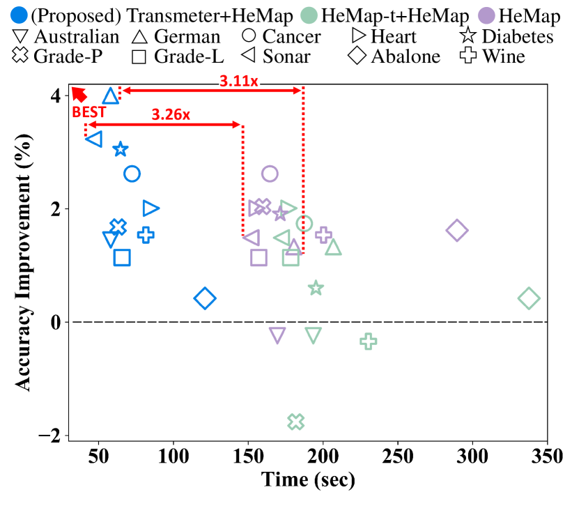
Figure 2: Using Transmeter to measure transferability, and fully transferring the selected data provides the best accuracy with the fastest running times.

2 Related Works

We review previous works on heterogeneous transfer learning, relevance of source data, and domain adversarial learning.

2.1 Heterogeneous Transfer Learning

Heterogeneous transfer learning aims for transferring knowledge between heterogeneous domains. However, different feature spaces and distributions impose significant challenges such as severe negative transfer. Recent studies to address these challenges are divided into two groups: symmetric and asymmetric feature-based transfer learning. Symmetric approaches transform both source and target domains into a common latent space (?, ?, ?) while asymmetric approaches transform only a source domain to a target domain (?, ?, ?). Transmeter belongs to the asymmetric feature-based transfer learning. Transmeter transforms the target domain into the dimension of the source domain to make homogeneous representations in the source domain. This asymmetric feature transformation enables Transmeter to reuse the pre-trained source classifier which accelerates its training.

2.2 Relevance of Source Data

The purpose of transfer learning is to improve the performance of a target learner by utilizing source data. However, the target learner can be negatively impacted if the source domain is weakly related to the target domain, which is referred to as negative transfer (?, ?). Hence, variant researches are performed to consider the relevance of source datasets in multi-source transfer learning (?, ?), or to select relevant source data (?) to avoid a negative transfer. Cao et al. propose Supervised Local Weight (SLW) scheme to attenuate the effect of irrelevant source dataset (?), and Wang et al. impose weights for each source data considering their relevance (?). Our proposed method Transmeter directly measures the transferability of each source dataset and enables us to find the most relevant one beyond merely avoiding the negative transfer.

2.3 Domain Adaptation

Domain adaptation aims to minimize the gap between source and target domains, which is crucial for the performance of the target learner after transferring source data. Ganin et al. propose Domain Adversarial Neural Network (DANN) that introduces the adversarial architecture of a domain classifier and a feature extractor (?); the domain classifier enforces the feature extractor to generate indistinguishable representations of source and target data. The adversarial architecture of a domain classifier and a feature extractor is utilized in various recent researches in transfer learning (?, ?, ?). Transmeter adopts the adversarial architecture of a target encoder and a domain classifier to reduce the domain gap between homogeneous representations of source and target datasets. Additionally, we introduce a target decoder that minimizes the reconstruction loss of the target data to make the target encoder extract meaningful homogeneous representations.

3 Proposed Method

In this section, we formally define the problem and propose Transmeter, a fast and accurate method for measuring transferability.

3.1 Problem Definition

We define the problem of selecting the best source for a given target task. Given a set $D_{s}=\{D_{s_{1}},...,D_{s_{N}}\}$ of $N$ source datasets with $N$ pre-trained models $F_{lp}=\{f_{lp_{1}},...,f_{lp_{N}}\}$ and a target dataset $D_{t}$, our objective is to find the best source data and its related classifier that improve the target accuracy the most after transferring them to the target task. We assume that all the pre-trained models have sufficient performance on their own domains. The $i$-th source dataset $D_{s_{i}}=\{(x^{j}_{s_{i}},y^{j}_{s_{i}})\}^{n_{s_{i}}}_{j=1}$ has $n_{s_{i}}$ samples while the target dataset $D_{t}=\{(x_{t}^{j},y_{t}^{j})\}^{n_{t}}_{j=1}$ has $n_{t}$ samples, where $x^{j}_{s_{i}}$ $\in$ $R^{d_{s_{i}}}$, $x_{t}^{j}$ $\in$ $R^{d_{t}}$, and $y_{s_{i}}^{j}$, $y_{t}^{j}$ $\in$ $\{0,1\}$. We focus on heterogeneous transfer learning where $d_{s_{i}}\neq d_{t}$, and binary classification.

To precisely evaluate the performance gain, we define the transferability we aim to optimize.

Definition 1 (Transferability)

Given a pair of a source and a target data, the transferability between them is defined as the ratio of accuracy improvement by transferring the source data for the target task.

$$Transferability=\frac{acc_{T}-acc_{0}}{acc_{0}}\times 100\ (\%)$$ (1)

where $acc_{T}$ and $acc_{0}$ represent the target accuracy with and without transferring the source data to the target task, respectively.

Figure 3: Transmeter consists of four modules: a target encoder that maps a target domain to a homogeneous domain, a target decoder that maps the homogeneous domain to the target domain, a label predictor for label prediction, and a domain classifier that classifies whether the data come from the source or the target domain. Transmeter aims to transform the target data such that they are indistinguishable from the source data.

3.2 Overview

Our proposed method Transmeter evaluates the transferability between source datasets $\{D_{s_{i}}\}$ and a target dataset $D_{t}$. After evaluating the transferability of each source dataset, we consider the one with the highest transferability as the best source data. As shown in Figure 3, Transmeter consists of four modules: target encoder $f_{en}$, target decoder $f_{de}$, label predictor $f_{lp}$, and domain classifier $f_{dc}$. We design Transmeter to address the following challenges on measuring transferability between two heterogeneous multivariate datasets.

• Reducing time. How can we quickly measure transferability to fully exploit the advantage of the transferability measurement algorithm?

• Minimizing the domain gap. It is more difficult to match two heterogeneous datasets than homogeneous datasets. How can we effectively reduce the domain gap between two heterogeneous datasets?

• Extracting meaningful target features. How can we keep the crucial features of the target instances for accurate classification, while minimizing the domain gap?

We address the aforementioned challenges by the following ideas:

• Reusing a pre-trained source model. We reuse the classifier pre-trained on the source data as the label predictor; this gives a better initialization for the label predictor, and reduces the training time of Transmeter.

• Domain adversarial network. We design a domain adversarial network that consists of a target encoder and a domain classifier to minimize the domain gap. The domain classifier aims to determine whether an instance comes from the source or the target domains. The target encoder generates homogeneous representations to confuse the domain classifier. This enables the target encoder to extract domain-invariant features which are fed into the label predictor to classify target instances.

• Encoder-decoder architecture. We introduce a target decoder, which forms an encoder-decoder architecture with the target encoder, that reconstructs the original target data from their homogeneous representations. Combined with the domain adversarial network, this makes the homogenous representations of target instances keep their crucial features while being indistinguishable from those of source instances in terms of label predictor’s point of view.

We design our objective function so that it includes the three main ideas above. We explain the details of our objective function in the following section.

3.3 Objective Function

We define our learning objective as follows:

$$\begin{split}E(\theta_{en},\theta_{de},\theta_{lp},\theta_{dc})=\frac{1}{n_{s}+n_{t}}\left[\sum^{n_{s}}_{i=1}L^{i}_{lp}(x^{i}_{s},y^{i}_{s};\theta_{en},\theta_{lp})+\sum^{n_{t}}_{i=1}L^{i}_{lp}(x^{i}_{t},y^{i}_{t};\theta_{en},\theta_{lp})\right]\\ -\alpha\cdot\frac{1}{n_{s}+n_{t}}\left[\sum^{n_{s}}_{i=1}L^{i}_{dc}(x^{i}_{s},d^{i}_{s};\theta_{en},\theta_{dc})+\sum^{n_{t}}_{i=1}L^{i}_{dc}(x^{i}_{t},d^{i}_{t};\theta_{en},\theta_{dc})\right]\\ +\beta\cdot\left[\frac{1}{n_{t}}\sum^{n_{t}}_{i=1}L^{i}_{r}(x^{i}_{t};\theta_{en},\theta_{de})\right]\end{split}$$ (2)

$\theta_{en}$, $\theta_{de}$, $\theta_{lp}$, and $\theta_{dc}$ are trainable parameters of the target encoder, the target decoder, the label predictor, and the domain classifier, respectively. The optimal parameters $\theta^{*}_{en}$, $\theta^{*}_{de}$, $\theta^{*}_{lp}$, and $\theta^{*}_{dc}$ satisfy

$$\begin{split}(\theta^{*}_{en},\theta^{*}_{de},\theta^{*}_{lp})&=\operatorname*{argmin}_{\theta_{en},\theta_{de},\theta_{lp}}E(\theta_{en},\theta_{de},\theta_{lp},\theta_{dc})\\ \theta^{*}_{dc}&=\operatorname*{argmax}_{\theta_{dc}}E(\theta_{en},\theta_{de},\theta_{lp},\theta_{dc})\\ \end{split}$$ (3)

The loss function $E$ in Equation 2 contains the loss terms $L^{i}_{lp}$ for the label predictor (Section 3.3.1), $L^{i}_{dc}$ for the domain classifier (Section 3.3.2), and $L^{i}_{r}$ for the target feature reconstruction (Section 3.3.3). $\alpha$ and $\beta$ are nonnegative hyperparameters that balance the loss terms. $x^{i}_{s}$, $x^{i}_{t}$, $y^{i}_{s}$, and $y^{i}_{t}$ denote features and labels of the $i$-th source and target instances, respectively. $d^{i}_{s}$ and $d^{i}_{t}$ are domain labels of $i$-th source instance and $i$-th target instance, respectively. $n_{s}$ and $n_{t}$ are the numbers of the source and the target instances, respectively.

3.3.1 Label Predictor

$$L^{i}_{lp}(x^{i},y^{i};\theta_{en},\theta_{lp})=-y^{i}\cdot log(\hat{y}^{i})-(1-y^{i})\cdot log(1-\hat{y}^{i})$$ (4)

$$\hat{y}^{i}=f_{lp}(Ho(x^{i};\theta_{en});\theta_{lp})$$ (5)

$$Ho(x^{i};\theta_{en})=\left\{\begin{array}[]{ll}x^{i}&if\ source\ data,\\ f_{en}(x^{i};\theta_{en})&otherwise\\ \end{array}\right.$$ (6)

$L^{i}_{lp}$ is the label predictor loss of the $i$-th instance. $\hat{y}^{i}$ (Equation 5) denotes the predicted label of the $i$-th instance. $Ho$ in Equation 6 denotes the homogeneous representation shown in Figure 3. $f_{lp}$ is the label predictor with parameter $\theta_{lp}$, and $f_{en}$ is the target encoder with parameter $\theta_{en}$.

3.3.2 Domain Classifier

The domain discrimination loss in Equation 7 is designed to improve the accuracy of the target label prediction by making the source and the target features indistinguishable.

$$L^{i}_{dc}(x^{i},d^{i};\theta_{en},\theta_{dc})=-d^{i}\cdot log(\hat{d}^{i})-(1-d^{i})\cdot log(1-\hat{d}^{i})$$ (7)

$$\hat{d}^{i}=f_{dc}(Ho(x^{i};\theta_{en});\theta_{dc})$$ (8)

$L^{i}_{dc}$ is the domain classifier loss of the $i$-th instance. $f_{dc}$ is the domain classifier with parameter $\theta_{dc}$, and $\hat{d}^{i}$ (Equation 8) denotes the predicted domain class of the $i$-th instance.

3.3.3 Feature Reconstruction

The feature reconstruction loss in Equation 9 is designed to extract useful features which are able to reconstruct the original target data. This can be thought of as an autoencoder where the encoder maps the input features into a constrained code, and the decoder recovers the code to the input features. The model is trained to minimize the reconstruction loss for each target data point.

$$L^{i}_{r}(x^{i};\theta_{en},\theta_{de})=||\hat{x}^{i}-x^{i}||^{2}$$ (9)

$$\hat{x}^{i}=f_{de}(Ho(x^{i};\theta_{en});\theta_{de})$$ (10)

$L^{i}_{r}$ is the feature reconstruction loss of the $i$-th instance. $f_{de}$ is the domain classifier with parameter $\theta_{de}$, and $\hat{x}^{i}$ in Equation 10 denotes the reconstructed feature of the $i$-th instance.

3.4 Transmeter

Given a source dataset with its pre-trained model, and a target dataset, Transmeter learns the model parameters $\theta_{en}$, $\theta_{de}$, $\theta_{lp}$, and $\theta_{dc}$ to measure the transferability. Note that the parameters of the pre-trained source model are used for initializing the weight $\theta_{lp}$ of the label predictor. In the training process, both the source and the target data are used to update the parameters.

We also consider the correspondence between labels of the source and the target data to maximize the performance of Transmeter. We observe that 0-labeled source data often correspond to 1-labeled target data rather than 0-labeled target data. Thus, we design a hyperparameter for flipping target labels, and find the better alignment of labels by training twice for each source and target pair of datasets: flipping or not flipping target labels.

4 Experiments

We conduct experiments to answer the following questions on the performance of Transmeter.

• Q1. Accuracy of transferability (Section 4.2). Does Transmeter accurately predict the best source data?

• Q2. Training time for transferability (Section 4.3). How much training time is saved by using Transmeter for transferability measurement?

• Q3. Exploiting transferability for full transfer (Section 4.4). How useful is Transmeter for transfer learning with multiple source candidates?

• Q4. Ablation study (Section 4.5). Does using a pre-trained source model and reconstruction loss improve the performance of Transmeter?

4.1 Experimental Settings

We describe experimental settings including datasets and competitors. All codes are written in python 3.6 using PyTorch, and all experiments are done in a workstation with Geforce GTX 1080 Ti.

Datasets.

We use ten multivariate datasets for binary classification summarized in Table 1: Australian, German, Cancer, Heart, Diabetes, Grade-P, Grade-L, Sonar, Abalone, and Wine. Note that all the datasets are heterogeneous; they have different categories and lie on different feature spaces. We split each data into training and test sets by 7:3 ratio, and preprocess them using z-normalization.

Data Name	Abbr.	Category	Features	Instances
Australian Credit Approval	Australian	Financial	14	690
German Credit data	German	Financial	24	1000
Breast Cancer Wisconsin (Diagnostic)	Cancer	Health	30	569
Heart Disease Data Set	Heart	Health	13	303
Pima Indians Diabetes Database	Diabetes	Health	8	768
Student Grade Prediction (Portugese)	Grade-P	Education	32	395
Student’ Academic Performance Dataset	Grade-L	Education	16	480
Connectionist Bench (Sonar, Mines vs. Rocks)	Sonar	Science	60	208
Abalone Data set	Abalone	Science	8	4177
Red Wine Quality	Wine	Science	11	1599

Table 1: Summary of the datasets.

Competitors.

We use HeMap (?) and its variant as competitors. HeMap (?) is the most recent heterogeneous transfer learning method for multivariate data. It samples source data points near target data points and determines that it is too risky to transfer when the ratio of the selected source data is lower than a threshold. We exploit this ratio of the selected source data as a transferability between two datasets and name this method as HeMap-t. We utilize HeMap for fully transferring source data after finding the best source data and leverage HeMap-t for a competitor of Transmeter as a transferability measurement algorithm.

Hyperparameters.

We use four or five hidden layers for pre-trained source models, three or four hidden layers for the target encoder, and a single layer for the domain classifier. The architecture of the target decoder is symmetric to that of the target encoder, and the label predictor has the identical structure with the pre-trained source model. We use MLPs for all modules since we focus on multivariate data and apply He-initialization (?), ReLU activation, and batch normalization as a default setting for each layer. We select the best values of $\alpha$ and $\beta$ among $\alpha\in$ $\{$0.003, 0.01, 0.1, 0.3, 1.0, 10.0$\}$ and $\beta\in\{0.1,0.5\}$ to balance the loss terms for each dataset; we use a larger set for $\alpha$ than $\beta$ since Transmeter is sensitive more to the domain classifier. We select the best random seed among $\{1,2,3,4,5\}$ to initialize random functions. We perform 3-fold cross-validation to select the best set of hyperparameters and use Adam optimizer for training all methods.

4.2 Accuracy of Transferability

We evaluate the transferability of Transmeter and the competing method HeMap-t. We measure the transferability of each source data and select the top $k$ sources ($k=1..4$); more than $k$ sources may be selected when the scores are the same. Then, we check if the pool of selected source datasets includes the best source for HeMap, the full transfer method. The results are summarized in Table 2 where the 2nd and the 3rd rows denote the number of correctly predicted best source models for 10 target datasets by utilizing Transmeter and HeMap-t, respectively. For each target dataset, we use the other datasets as sources. Note that Transmeter outperforms HeMap-t in all cases, correctly finding the best source data in 80% or 90% of cases in Top-2, 3, 4 settings.

Additionally, we count the number of cases that target labels are flipped when we train the final model to verify the effect of label matching. As a result, almost half of total cases (95 cases among 180 cases) show better performance when they are trained with flipped labels. Thus, it is worthwhile to train each pair of source and target data twice with flipped and unflipped target labels considering the relationship between source and target labels.

Methods	Top-1	Top-2	Top-3	Top-4
Transmeter	5/10	8/10	8/10	9/10
HeMap-t	4/10	5/10	7/10	9/10

Table 2: Ratio of target tasks where their best source data are included in the top-$k$ sources found by transferability measurement methods. Transmeter outperforms HeMap-t in all cases.

4.3 Training Time

Figure 2 shows the comparison of training times of Transmeter and competitors. We use an early stopping technique for training each model; we stop training when the number of consecutive epochs with increasing validation loss surpasses a threshold. Note that Transmeter shows up to 10.3 $\times$ faster training time than the second-best competitor HeMap-t. The short training time of Transmeter enables measuring the transferability of all source candidates before performing a full transfer.

4.4 Exploiting Transferability for Full Transfer

We evaluate how to exploit the transferability for quickly and accurately improving a target task via full transfer. There are two ways to quickly increase the accuracy of the target task. First, we can use a transferability measurement method to find the best source, and use a full transfer algorithm to transfer the best source data to the target task. Second, we can use a full transfer method to fully transfer all source data, and find the best one among them. Thus, we compare the following three settings. Note that we use 1) HeMap as a full-transfer method, and 2) Transmeter and HeMap-t as transferability measurement methods.

• (Proposed) Transmeter + HeMap. We measure the transferability of each source data using Transmeter, and select the top two source data; we include all the source data when there are multiple data with the same ranking. We then transfer the selected source data to the target task using HeMap. Although Transmeter is designed as a transferability measurement method, Transmeter can be used for full transfer as well; thus we choose the best model among the ones trained by HeMap and Transmeter.

• HeMap-t + HeMap. We measure the transferability of each source data using HeMap-t, and select the top two source data; we include all the source data when there are multiple data with the same ranking. We then transfer the selected source data to the target task using HeMap. Note that HeMap-t is not used for full transfer since it is designed only for transferability measurement.

• HeMap. We fully transfer all source data one by one using HeMap, and find the best model among them.

The results of the experiments are shown in Figure 2 where each color represents a method, and each symbol represents a target dataset. The vertical axis represents the improvement of the target accuracy compared to the baseline trained only with each target data. Note that using Transmeter as a transferability measurement method provides the best accuracy while minimizing running times. Transmeter always gives better or equal accuracy in identifying the best source data compared to HeMap-t, with faster running times. Transmeter combined with HeMap also provides better accuracy and smaller running times compared to an exhaustive search using only HeMap; Transmeter +HeMap gives better or equal accuracy in 8 out of 10 cases, while running up to 3.26$\times$ faster than HeMap.

4.5 Ablation Study

We conduct an ablation study to verify the contribution of using a pre-trained source model and the reconstruction loss (Equation 9). We compare the training times and top-2 accuracy of Transmeter with its following two variants. Transmeter-S is a variant of Transmeter that does not initialize weights of label predictor using a pre-trained source model; instead, Transmeter-S uses the default initialization method (?) for linear layers in PyTorch. Transmeter-R is a variant of Transmeter trained without the reconstruction loss. The result of ablation study in Table 3 explicitly shows that using the pre-trained source model for weight initialization accelerates the training of the Transmeter with better accuracy, and introducing the reconstruction loss greatly increases the accuracy of measuring transferability.

Methods	Top-2 Acc.	Training Time (sec)
Transmeter	8/10	2.78
Transmeter-S	7/10	7.87
Transmeter-R	2/10	2.25

Table 3: Transmeter gives the best trade-off of accuracy and training time, compared to its variants without the pre-trained source model (-S) and without the reconstruction loss (-R).

5 Conclusion

In this paper, we propose Transmeter, a novel algorithm that measures the transferability between two heterogeneous multivariate datasets. We exploit a pre-trained source model as a label predictor to reduce the training time, an adversarial network to reduce the gap between the source and the target domains, and an encoder-decoder architecture to extract meaningful homogeneous representations. Extensive experiments on heterogeneous multivariate data demonstrate that 1) Transmeter provides the most accurate transferability measurement with up to 10.3$\times$ faster training time than its competitor, and 2) using Transmeter to measure the transferability and fully transferring the selected data provides the best accuracy with the fastest running times. Future works encompass extending the method for simultaneously transferring multiple heterogeneous source data.

Acknowledgments

This work is supported by SAMSUNG Research, Samsung Electronics Co.,Ltd.

References

- Cao, Long, Wang, & Jordan Cao, Z., Long, M., Wang, J., & Jordan, M. I. (2018). Partial transfer learning with selective adversarial networks. In 2018 IEEE Conference on Computer Vision and Pattern Recognition, CVPR 2018, Salt Lake City, UT, USA, June 18-22, 2018, pp. 2724–2732.
- Chen, Chen, Chen, Tsai, Wang, & Sun Chen, Y., Chen, W., Chen, Y., Tsai, B., Wang, Y. F., & Sun, M. (2017). No more discrimination: Cross city adaptation of road scene segmenters. In IEEE International Conference on Computer Vision, ICCV 2017, Venice, Italy, October 22-29, 2017, pp. 2011–2020.
- Duan, Xu, & Chang Duan, L., Xu, D., & Chang, S. (2012a). Exploiting web images for event recognition in consumer videos: A multiple source domain adaptation approach. In 2012 IEEE Conference on Computer Vision and Pattern Recognition, Providence, RI, USA, June 16-21, 2012, pp. 1338–1345. IEEE Computer Society.
- Duan, Xu, & Tsang Duan, L., Xu, D., & Tsang, I. W. (2012b). Learning with augmented features for heterogeneous domain adaptation. In Proceedings of the 29th International Conference on Machine Learning, ICML 2012, Edinburgh, Scotland, UK, June 26 - July 1, 2012.
- Ganin, Ustinova, Ajakan, Germain, Larochelle, Laviolette, Marchand, & Lempitsky Ganin, Y., Ustinova, E., Ajakan, H., Germain, P., Larochelle, H., Laviolette, F., Marchand, M., & Lempitsky, V. S. (2017). Domain-adversarial training of neural networks. In Domain Adaptation in Computer Vision Applications, pp. 189–209.
- Gong, Shi, Sha, & Grauman Gong, B., Shi, Y., Sha, F., & Grauman, K. (2012). Geodesic flow kernel for unsupervised domain adaptation. In 2012 IEEE Conference on Computer Vision and Pattern Recognition, Providence, RI, USA, June 16-21, 2012, pp. 2066–2073.
- He, Zhang, Ren, & Sun He, K., Zhang, X., Ren, S., & Sun, J. (2015). Delving deep into rectifiers: Surpassing human-level performance on imagenet classification. In 2015 IEEE International Conference on Computer Vision, ICCV 2015, Santiago, Chile, December 7-13, 2015, pp. 1026–1034. IEEE Computer Society.
- Hoffman, Wang, Yu, & Darrell Hoffman, J., Wang, D., Yu, F., & Darrell, T. (2016). Fcns in the wild: Pixel-level adversarial and constraint-based adaptation. CoRR, abs/1612.02649.
- III III, H. D. (2007). Frustratingly easy domain adaptation. In ACL 2007, Proceedings of the 45th Annual Meeting of the Association for Computational Linguistics, June 23-30, 2007, Prague, Czech Republic.
- Kulis, Saenko, & Darrell Kulis, B., Saenko, K., & Darrell, T. (2011). What you saw is not what you get: Domain adaptation using asymmetric kernel transforms. In The 24th IEEE Conference on Computer Vision and Pattern Recognition, CVPR 2011, Colorado Springs, CO, USA, 20-25 June 2011, pp. 1785–1792.
- Li, Duan, Xu, & Tsang Li, W., Duan, L., Xu, D., & Tsang, I. W. (2014). Learning with augmented features for supervised and semi-supervised heterogeneous domain adaptation. IEEE Trans. Pattern Anal. Mach. Intell., 36(6), 1134–1148.
- Long, Cao, Wang, & Jordan Long, M., Cao, Z., Wang, J., & Jordan, M. I. (2018). Conditional adversarial domain adaptation. In Advances in Neural Information Processing Systems 31: Annual Conference on Neural Information Processing Systems 2018, NeurIPS 2018, 3-8 December 2018, Montréal, Canada, pp. 1647–1657.
- Oquab, Bottou, Laptev, & Sivic Oquab, M., Bottou, L., Laptev, I., & Sivic, J. (2014). Learning and transferring mid-level image representations using convolutional neural networks. In 2014 IEEE Conference on Computer Vision and Pattern Recognition, CVPR 2014, Columbus, OH, USA, June 23-28, 2014, pp. 1717–1724.
- Pan, Ni, Sun, Yang, & Chen Pan, S. J., Ni, X., Sun, J., Yang, Q., & Chen, Z. (2010). Cross-domain sentiment classification via spectral feature alignment. In Proceedings of the 19th International Conference on World Wide Web, WWW 2010, Raleigh, North Carolina, USA, April 26-30, 2010, pp. 751–760.
- Rosenstein, Marx, & Kaebling Rosenstein, M. T., Marx, Z., & Kaebling, L. P. (2005). To transfer or not to transfer. In NIPS 2005 workshop on transfer learning, Vol. 898, pp. 1–4.
- Shi, Liu, Fan, Yu, & Zhu Shi, X., Liu, Q., Fan, W., Yu, P. S., & Zhu, R. (2010). Transfer learning on heterogenous feature spaces via spectral transformation. In 2010 IEEE International Conference on Data Mining, pp. 1049–1054.
- Wang & Mahadevan Wang, C., & Mahadevan, S. (2011). Heterogeneous domain adaptation using manifold alignment. In IJCAI 2011, Proceedings of the 22nd International Joint Conference on Artificial Intelligence, Barcelona, Catalonia, Spain, July 16-22, 2011, pp. 1541–1546.
- Wang, Dai, Póczos, & Carbonell Wang, Z., Dai, Z., Póczos, B., & Carbonell, J. G. (2018). Characterizing and avoiding negative transfer. CoRR, abs/1811.09751.
- Weiss, Khoshgoftaar, & Wang Weiss, K. R., Khoshgoftaar, T. M., & Wang, D. (2016). A survey of transfer learning. J. Big Data, 3, 9.
- Yan, Li, Ng, Tan, Wu, Min, & Wu Yan, Y., Li, W., Ng, M. K. P., Tan, M., Wu, H., Min, H., & Wu, Q. (2017). Learning discriminative correlation subspace for heterogeneous domain adaptation. In Proceedings of the Twenty-Sixth International Joint Conference on Artificial Intelligence, IJCAI 2017, Melbourne, Australia, August 19-25, 2017, pp. 3252–3258.
- Yao & Doretto Yao, Y., & Doretto, G. (2010). Boosting for transfer learning with multiple sources. In The Twenty-Third IEEE Conference on Computer Vision and Pattern Recognition, CVPR 2010, San Francisco, CA, USA, 13-18 June 2010, pp. 1855–1862.
- Ye, Sheng, Zhan, & He Ye, H., Sheng, X., Zhan, D., & He, P. (2018). Distance metric facilitated transportation between heterogeneous domains. In Proceedings of the Twenty-Seventh International Joint Conference on Artificial Intelligence, IJCAI 2018, July 13-19, 2018, Stockholm, Sweden, pp. 3012–3018.
- Zhou, Tsang, Pan, & Tan Zhou, J. T., Tsang, I. W., Pan, S. J., & Tan, M. (2014). Heterogeneous domain adaptation for multiple classes. In Proceedings of the Seventeenth International Conference on Artificial Intelligence and Statistics, AISTATS 2014, Reykjavik, Iceland, April 22-25, 2014, pp. 1095–1103.