Learning Representations by Maximizing Mutual Information in Variational Autoencoders

Abstract

Variational autoencoders (VAEs) have ushered in a new era of unsupervised learning methods for complex distributions. Although these techniques are elegant in their approach, they are typically not useful for representation learning. In this work, we propose a simple yet powerful class of VAEs that simultaneously result in meaningful learned representations. Our solution is to combine traditional VAEs with mutual information maximization, with the goal to enhance amortized inference in VAEs using Information Theoretic techniques. We call this approach InfoMax-VAE, and such an approach can significantly boost the quality of learned high-level representations. We realize this through the explicit maximization of information measures associated with the representation. Using extensive experiments on varied datasets and setups, we show that InfoMax-VAE outperforms contemporary popular approaches, including Info-VAE and $\beta$-VAE.

1 Introduction

There is growing interest in generative models, with new powerful tools being developed for modeling complex data and reasoning under uncertainty pu2016deep ; radford2015unsupervised ; NIPS2016_6066 . Simultaneously, there is significant interest and progress being made in learning representations of high-dimensional data such as images hjelm2018learning . Particularly, the development of variational autoencoders kingma2013auto has enabled many applications, ranging from image processing to language modeling bowman2015generating ; pu2016variational ; xu2018spherical . VAEs have also found use as a representation learning model for inferring latent variables tschannen2018recent .

Although successful for multiple isolated applications, VAEs have not always proven to be reliable for extracting high-level representations of observations alemi2017fixing ; pmlr-v89-dieng19a . As generative networks become more descriptive/richer, the extraction of meaningful representations becomes considerably more challenging. Overall, VAEs can often fail to take the advantage of its underlying mixture model, and the learned features can lose their dependencies on observations. Overall, VAEs alone may not be adequate in ensuring that the representation is accurate. In many practical applications, problem-specific solutions are presented, and our goal is to build a more general framework to build meaningful, useful representations with VAEs.

In this work, we present a simple but powerful method to train VAEs with associated guarantees towards the usefulness of learned high-level (latent) representations, by evaluating them on the basis of various metrics. Our main idea is to induce the maximization of mutual information (between the learned latent representations and input) into the VAE objective. We call our resulting solution an InfoMax-VAE as we seek to distill the information resulting from the input data into the latent codes to the highest extent possible. To this end, we formalize the development of InfoMax-VAE: As a first step, we develop a computationally tractable optimization problem. Indeed, it simultaneously acts as an autoencoder while estimating and maximizing the mutual information between input data and the resulting representation(s). We study the performance of InfoMax-VAE on different datasets across different setting to prove its advantages over other well-known approaches.

2 Related Work

The variational autoencoder was first proposed in kingma2013auto ; rezende2014stochastic . VAEs are designed to jointly optimize a pair of networks: a generative network and an inference network. There are many popular approaches to enhance the performance of VAEs for particular settings. Adversarial autoencoders (AAE) makhzani2015adversarial , and adversarial regularized autoencoders (ARAE) zhao2017adversarially are VAE-based methods proposed to leverage adversarial learning goodfellow2014generative . Indeed, both VAE and AAE have similar goals but utilize different approaches to match the posterior with the prior. $\beta$-VAE higgins2017beta is another variant for VAE, where the regularizer (the KL divergence between the amortized inference distribution and prior) is amplified by $\beta$. Using this, inferred high-level abstractions become more disentangled where the effect of varying each latent code is transparent.

There are several papers that discuss the issue of latent variable collapse alemi2017fixing ; chen2016variational ; zhao2017towards . In one thread of research, bowman2015generating ; pmlr-v70-yang17d weaken and restrict the capacity of a generative network to enable higher-quality learned representations. Another proposed mechanism is to substitute simplistic priors with more sophisticated priors which encourage the model to learn features of interest. For example NIPS2017_7210 suggests a parametric prior whose parameters are trained via a generative model. Other approaches use richer models with further modifications into the model. For example NIPS2017_7133 ; NIPS2017_7020 replace the KL divergence with the Jensen-Shannon divergence which enables the data and latent codes to be treated in a symmetric manner. In both studies adversarial training is leveraged to estimate the Jensen-Shannon divergence.

There is also a recent body of work that works towards enabling the maximization of the mutual information in VAEs. For example, pmlr-v89-dieng19a suggests several skip connections from the latent codes to the output of VAE to implicitly force higher dependency between the latent codes and observations. In hoffman2016elbo , the authors propose to maximize the mutual information between learned latent representations and input data which is realized by adding mutual information to VAE objective. Their approach is to estimate $q_{\phi}(\boldsymbol{z})$ using Monte-Carlo and then calculate the mutual information. However, such an estimation is computationally expensive and also limits the performance benefits pmlr-v80-kim18b . With a similar goal, Info-VAE zhao2019infovae proposed to evade the calculation of mutual information by recasting the objective. In so doing, Info-VAE minimizes the MMD distance (or the KL divergence) between the marginal of the inference network and the prior to implicitly increase the corresponding mutual information contained in the model. Thus, Info-VAE effectively becomes a mixture of AAE and $\beta$-VAE. Using Info-VAE, the best results are achieved once the adversarial learning in AAE is replaced by the maximum-mean discrepancy. Also, Info-VAE is limited in the choice of information preference; see Appendix A for more details. In our work, however, we explicitly estimate and maximize the mutual information with means of another deep neural network, and it offers much greater flexibility in the selection of the mutual information coefficient. Also, we believe this flexibility is the primary reason why InfoMax-VAE outperforms InfoVAE in all models and datasets, as we enable the resulting VAE to uncover more information-rich latent codes compared to InfoVAE.

3 Background and Notation

Following the same lines as the literature on variational inference, we assume that we have a set of observed data $\boldsymbol{X}=\{\boldsymbol{x}^{(i)}\}_{i=1}^{N}$, consisting of $N$ i.i.d. samples $\boldsymbol{x}$. Indeed, these samples are assumed to come from a distribution $q(\boldsymbol{x})$, where we have access to its empirical distribution rather than its explicit form. We assume that samples are being drawn from the posterior $p_{\theta}(\boldsymbol{x}|\boldsymbol{z})$, with $\theta$ as the generative model parameters and $\boldsymbol{z}$ is the hidden latent variable (latent features, representations, or high-level abstraction). The prior distribution is denoted by $p(\boldsymbol{z})$ and the amortized inference distribution by $q_{\phi}(\boldsymbol{z}|\boldsymbol{x})$ (it is also called variational posterior distribution), which is used to map the data to latent variable space, and $p_{\theta}(\boldsymbol{x}|\boldsymbol{z})$ enables us to return to the input data space. Naturally, $q_{\phi}(\boldsymbol{z}|\boldsymbol{x})$ is called the encoder or inference model, while $p_{\theta}(\boldsymbol{x}|\boldsymbol{z})$ refers to the decoder or generative model. Importantly, the variational posterior distributions are typically designed for easy sampling, and are often modeled using deep neural networks. VAEs seek to maximize the variational expression for maximum likelihood: $\mathcal{L}_{\phi,\theta}$ with respect to parameters $\phi$ and $\theta$, where we have:

$$\begin{split}&\mathcal{L}_{\text{VAE}}(\phi,\theta)=\\ &\mathbb{E}_{q{(\boldsymbol{x})}}[\mathbb{E}_{q_{\phi}(\boldsymbol{z}|\boldsymbol{x})}[\log p_{\theta}(\boldsymbol{x}|\boldsymbol{z})]-\text{KL}(q_{\phi}(\boldsymbol{z}|\boldsymbol{x})||p(\boldsymbol{z}))]\\ &=-\text{KL}(q_{\phi}(\boldsymbol{x},\boldsymbol{z})||p_{\theta}(\boldsymbol{x},\boldsymbol{z}))]+\text{const}.\end{split}$$ (1)

The expectations $\mathbb{E}_{q{(\boldsymbol{x})}}$ and $\mathbb{E}_{q_{\phi}(\boldsymbol{z}|\boldsymbol{x})}$ are empirically approximated via sampling, where samples are drawn based on $\boldsymbol{x}^{(i)}\sim q(\boldsymbol{x})$ and $\boldsymbol{z}^{(i)}\sim q(\boldsymbol{z}|\boldsymbol{x})$, and the latter is realized via the reparameterization trick kingma2013auto . The associated KL divergence can be computed both analytically or using an approach similar to the one above. Likewise kingma2013auto , we call the first term in optimization as reconstruction error, while the KL divergence is interpreted as a regularizer.

4 Challenges in Meaningful/Useful Representations using VAEs

Although VAEs remain very popular for numerous applications ranging from image processing to language modeling, they typically suffer from challenges in enabling meaningful and useful representations $\boldsymbol{z}$. Indeed, under appropriate situations (where the sets $\theta$ and $\phi$ are defined appropriately) both inference and generative models collaborate in producing an acceptable $p_{\theta}(\boldsymbol{x}|\boldsymbol{z})$ and an accurate amortized inference. However, finding suitable models for inference and generative networks across different tasks and datasets is challenging - when the generative model is expressive, a vanilla VAE sacrifices log-likelihood in favor of amortized inference chen2016variational . As a consequence, we obtain latent variables which are independent from the observed data, in fact, $q_{\phi}(\boldsymbol{z}|\boldsymbol{x})=q_{\phi}(\boldsymbol{z})$.

To understand the origin of this discrepancy, we must return to the original problem. Particularly, a maximum likelihood technique is leveraged to minimize the bound on the KL divergence between the true data distribution $q(\boldsymbol{x})$ and the model’s marginal distribution $p_{\theta}(\boldsymbol{x})$, $\text{KL}(q(\boldsymbol{x})||p_{\theta}(\boldsymbol{x}))$; whereas the quality of the latent variables only depends on $q_{\phi}(\boldsymbol{z}|\boldsymbol{x})$. Thus, myopic maximum likelihood without additional constraints on the posterior is insufficient when aiming to uncover relevant and information-rich latent variables.

In addition, ELBO imposes a regularizer over latent codes, $\text{KL}(q_{\phi}(\boldsymbol{z}|\boldsymbol{x})||p(\boldsymbol{z}))$, where it seeks in the family set of $\phi$ for those solutions that minimize this KL divergence. As a result, it also reduces the usefulness of latent codes by encouraging $q_{\phi}(\boldsymbol{z}|\boldsymbol{x})$ to be matched to $p(\boldsymbol{z})$, which bears no relationship with observed data. Such an approach minimizes the upper bound of the mutual information between the representations and input data. To observe this, note that

$$\begin{split}\mathbb{E}_{q(\boldsymbol{x})}&[\text{KL}(q_{\phi}(\boldsymbol{z}|\boldsymbol{x})||p(\boldsymbol{z}))]=\int q_{\phi}(\boldsymbol{x},\boldsymbol{z})\log\frac{q_{\phi}(\boldsymbol{z}|\boldsymbol{x})}{p(\boldsymbol{z})}d\boldsymbol{x}d\boldsymbol{z}\\ &\geq\int q_{\phi}(\boldsymbol{x},\boldsymbol{z})\log\frac{q_{\phi}(\boldsymbol{z}|\boldsymbol{x})}{p(\boldsymbol{z})}d\boldsymbol{x}d\boldsymbol{z}-\text{KL}(q_{\phi}(\boldsymbol{z})||p(\boldsymbol{z}))\\ &=\int q_{\phi}(\boldsymbol{x},\boldsymbol{z})[\log\frac{q_{\phi}(\boldsymbol{z}|\boldsymbol{x})}{p(\boldsymbol{z})}-\log\frac{q_{\phi}(\boldsymbol{z})}{p(\boldsymbol{z})}]d\boldsymbol{x}d\boldsymbol{z}\\ &=\int q_{\phi}(\boldsymbol{x},\boldsymbol{z})\log\frac{q_{\phi}(\boldsymbol{z}|\boldsymbol{x})}{q_{\phi}(\boldsymbol{z})}\\ &=I_{q_{\phi}}(\boldsymbol{x};\boldsymbol{z}).\end{split}$$ (2)

The inequity arises from the fact that the KL divergence does not take negative values. Hence, as vanilla VAEs push the model to minimize the KL divergence between the variational posterior $q_{\phi}(\boldsymbol{z}|\boldsymbol{x})$ and prior $p(\boldsymbol{z})$, they also force the representations to carry less information from input data. Actually, this may potentially result in very poor learned representations. In practice, by employing expressive generative networks, the problem is exacerbated as the model sacrifices the inference in favor of the the likelihood. Indeed, the model becomes capable of recovering data from noise, regardless of latent codes. Therefore, a vanilla VAE may not be enough to discover accurate high-level abstractions of input data.

5 Representation Learning using VAE

5.1 InfoMax Variational Autoencoders

As discussed earlier, VAEs without additional constraints can prove to be unreliable for representation learning. One reason, as showed, is that the mutual information is not regarded in their objective appropriately. This bring us to the point to begin a new family of VAEs, so called InfoMax-VAE that effectively mitigates this issue by putting forth the explicit maximization of the mutual information between representations and data into VAEs. Therefore, we have an optimization problem of form,

$$\begin{split}\max_{\phi,\theta}\mathbb{E}_{q{(\boldsymbol{x})}}[\mathbb{E}_{q_{\phi}(\boldsymbol{z}|\boldsymbol{x})}[\log p_{\theta}(\boldsymbol{x}|\boldsymbol{z})]-&\beta\text{KL}(q_{\phi}(\boldsymbol{z}|\boldsymbol{x})||p(\boldsymbol{z}))]\\ +&\alpha I_{q_{\phi}}(\boldsymbol{x};\boldsymbol{z}),\end{split}$$ (3)

where $\beta,\alpha\geq 0$ are defined to be regularization coefficients for the KL divergence and mutual information. Varying $\alpha$ changes the amount of information in inferring representations. Please see the Appendix A for further explanation on the interpretation of the objective. Now, evaluating $I_{q_{\phi}}(\boldsymbol{x};\boldsymbol{z})$ is, in general, computationally challenging and intractable since it involves mixtures of a large number of components $q_{\phi}(\boldsymbol{z})=\int q_{\phi}(\boldsymbol{x},\boldsymbol{z})d\boldsymbol{x}$. Another key question is how to effectively estimate the mutual information by drawing samples from the joint and marginals, which will be addressed in the following subsection.

5.2 Dual Form of Mutual Information

We start the discussion with noting that mutual information is the KL divergence between the joint and associated marginals: $I_{q_{\phi}}(\boldsymbol{x};\boldsymbol{z})=\text{KL}(q_{\phi}(\boldsymbol{x};\boldsymbol{z})||q(\boldsymbol{x})q_{\phi}(\boldsymbol{z}))$. Interestingly, we can replace this KL divergence with any other strict divergences , $D$, which might prove to be better suited from an algorithmic perspective. In doing so, we can maximize other distances between the joint and marginals.

$$\begin{split}\max_{\phi,\theta}\mathbb{E}_{q{(\boldsymbol{x})}}[\mathbb{E}_{q_{\phi}(\boldsymbol{z}|\boldsymbol{x})}[\log p_{\theta}(\boldsymbol{x}|&\boldsymbol{z})]-\beta\text{KL}(q_{\phi}(\boldsymbol{z}|\boldsymbol{x})||p(\boldsymbol{z}))]\\ +&\alpha D(q_{\phi}(\boldsymbol{x};\boldsymbol{z})||q(\boldsymbol{x})q_{\phi}(\boldsymbol{z})).\end{split}$$ (4)

For instance, if we choose $f$-divergence, a large class of different divergences which includes the KL divergence, we get an alternate optimization problem, and by substituting the variational $f$-divergence we will have an objective of form:

$$\begin{split}\max_{\phi,\theta}\mathbb{E}_{q{(\boldsymbol{x})}}[&\mathbb{E}_{q_{\phi}(\boldsymbol{z}|\boldsymbol{x})}[\log p_{\theta}(\boldsymbol{x}|\boldsymbol{z})]-\beta\text{KL}(q_{\phi}(\boldsymbol{z}|\boldsymbol{x})||p(\boldsymbol{z}))]\\ +&\alpha D_{f}(q_{\phi}(\boldsymbol{x},\boldsymbol{z})||q(\boldsymbol{x})q_{\phi}(\boldsymbol{z})),\\ \\ =\max_{\phi,\theta}\mathbb{E}_{q{(\boldsymbol{x})}}[&\mathbb{E}_{q_{\phi}(\boldsymbol{z}|\boldsymbol{x})}[\log p_{\theta}(\boldsymbol{x}|\boldsymbol{z})]-\beta\text{KL}(q_{\phi}(\boldsymbol{z}|\boldsymbol{x})||p(\boldsymbol{z}))]\\ +&\alpha\mathbb{E}_{q(\boldsymbol{x})q_{\phi}(\boldsymbol{z})}[f(\frac{q_{\phi}(\boldsymbol{x},\boldsymbol{z})}{q(\boldsymbol{x})q_{\phi}(\boldsymbol{z})})],\\ \geq\max_{\phi,\theta,t}\mathbb{E}_{q{(\boldsymbol{x})}}[&\mathbb{E}_{q_{\phi}(\boldsymbol{z}|\boldsymbol{x})}[\log p_{\theta}(\boldsymbol{x}|\boldsymbol{z})]-\beta\text{KL}(q_{\phi}(\boldsymbol{z}|\boldsymbol{x})||p(\boldsymbol{z}))]\\ +&\alpha(\mathbb{E}_{q_{\phi}(\boldsymbol{x},\boldsymbol{z})}[t(\boldsymbol{x},\boldsymbol{z})]-\mathbb{E}_{q(\boldsymbol{x})q_{\phi}(\boldsymbol{z})}[f^{*}(t(\boldsymbol{x},\boldsymbol{z}))]),\end{split}$$ (5)

where $f^{*}$ is the convex conjugate function of $f$, and $t$ represents all possible functions. Such an inequality is imposed both due to Jensen’s inequality and due to the restriction on exploring all possible functions $t$. As a special case, if we take $f(t)$ to be $t\log t$, which corresponds to the KL divergence (or the mutual information between $\boldsymbol{x}$ and $\boldsymbol{z}$), we get the following dual representation for InfoMax-VAE,

$$\begin{split}\max_{\phi,\theta,t}&\mathbb{E}_{q{(\boldsymbol{x})}}[\mathbb{E}_{q_{\phi}(\boldsymbol{z}|\boldsymbol{x})}[\log p_{\theta}(\boldsymbol{x}|\boldsymbol{z})]-\beta\text{KL}(q_{\phi}(\boldsymbol{z}|\boldsymbol{x})||p(\boldsymbol{z}))]\\ +&\alpha(\mathbb{E}_{q_{\phi}(\boldsymbol{x},\boldsymbol{z})}[t(\boldsymbol{x},\boldsymbol{z})]-\mathbb{E}_{q(\boldsymbol{x})q_{\phi}(\boldsymbol{z})}[\exp(t(\boldsymbol{x},\boldsymbol{z})-1)]).\end{split}$$ (6)

To evaluate $\mathbb{E}_{q_{\phi}(\boldsymbol{x},\boldsymbol{z})}$ and $\mathbb{E}_{q(\boldsymbol{x})q_{\phi}(\boldsymbol{z})}$ in a tractable manner, we take an alternative approach. First, we observe that we can simply draw samples from $(\boldsymbol{x}^{(i)},\boldsymbol{z}^{(i)})\sim q_{\phi}(\boldsymbol{x};\boldsymbol{z})=q_{\phi}(\boldsymbol{z}|\boldsymbol{x})q(\boldsymbol{x})$ thanks to the reparameterization trick and having access to the empirical distribution of input data $q(\boldsymbol{x})=\frac{1}{N}\sum\delta_{\boldsymbol{x}^{(i)}}(\boldsymbol{x})$. Also to get samples from the marginal $q_{\phi}(\boldsymbol{z})$ we can randomly choose a datapoint $\boldsymbol{x}^{(j)}$ then sample from $\boldsymbol{z}\sim q_{\phi}(\boldsymbol{z}|\boldsymbol{x}^{(j)})$. In practice, however, we can effectively get samples from a batch and then permute representations $\boldsymbol{z}$ across the batch. This trick is first used in arcones1992bootstrap , and proved to be sufficiently accurate as long as the batch size is large enough, i.e., 64.

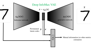
Figure 1: Architecture of InfoMax-VAE, a family of VAEs which encourages VAEs to learn useful high-level representations of data, the top networks can be convolutional or FC NNs. The bottom network ($t(\boldsymbol{x},\cdot)$) is an MLP which estimates the mutual information between inferred latent representations $\boldsymbol{z}$ and input data $\boldsymbol{x}$. Or, it can estimate any other strict divergence/distance between joint $q_{\phi}(\boldsymbol{x},\boldsymbol{z})$ and the marginals $q(\boldsymbol{x}),q_{\phi}(\boldsymbol{z})$.

Algorithm 1 InfoMax-VAE

1:$\mathcal{B}$ as a batch size of $b$, latent variable dimension $\boldsymbol{z}_{\text{dim}}$, $\alpha$, observations $\{\boldsymbol{x}\}_{i=1}^{N}$, VAE/Mutual information optimizers: $G$, $G_{t}$

2:Initialize $\phi$, $\theta$, $t$

3:repeat

4:     Randomly select $b$ observed datapoints from $\{\boldsymbol{x}\}_{i=1}^{b}$

5:     Get samples of $\boldsymbol{z}^{(i)}\sim q_{\phi}(\boldsymbol{z}|\boldsymbol{x}^{(i)})$, form $\{{(\boldsymbol{x},\boldsymbol{z}})\}_{i=1}^{b}$,

6:     permute latent codes $\{\boldsymbol{z}\}_{i=1}^{b}$ to get ${\{(\boldsymbol{x},\tilde{\boldsymbol{z}}})\}_{i=1}^{b}$

7:     $\theta,\phi\leftarrow G(\nabla_{\theta,\phi}[\frac{1}{b}\sum_{i=1}^{b}\log\frac{p_{\theta}(\boldsymbol{x}^{(i)}|\boldsymbol{z}^{(i)})p(\boldsymbol{z})^{\beta}}{q_{\phi}(\boldsymbol{z}^{(i)}|\boldsymbol{x}^{(i)})^{\beta}}+\frac{\alpha}{b}(\sum_{i=1}^{b}t(\boldsymbol{x}^{(i)},\boldsymbol{z}^{(i)})-\sum_{i=1}^{b}f^{*}(t(\boldsymbol{x}^{(i)},\tilde{\boldsymbol{z}}^{(i)}))]))$

8:     $t\leftarrow G_{t}(\nabla_{t}[\frac{1}{b}\sum_{i=1}^{b}t(\boldsymbol{x}^{(i)},\boldsymbol{z}^{(i)})-\frac{1}{b}\sum_{i=1}^{b}f^{*}(t(\boldsymbol{x}^{(i)},\tilde{\boldsymbol{z}}^{(i)}))])$

9:until convergence

Finally, while $f$-divergence family offers a large class of different divergences, our proposed method is also capable of taking other divergence families or other dual representations which might enable tighter bounds. As an example, we can also use Donsker-Varadhan dual representation for the KL divergence. In doing so, we obtain a tighter lower bound than $f$-dual representation for the KL divergence. See the Appendix C for more details. A detailed description of InfoMax-VAE approach is presented in Algorithm 1 and Figure 1.

6 Results

In this section, we evaluate our proposed InfoMax-VAE, and demonstrate that it consistently discovers more efficient high-level representations compared to other well-known approaches. To this end, we conduct experiments across the following datasets to compare the behavior of InfoMax-VAE against vanilla VAEs and its variant frameworks: 1) MNIST: 60,000 gray scale 28x28 images, 2) Binarized MNIST: the binary version of MNIST, 3) Fashion MNIST: 60,000 gray scale 28x28 images, 4) CIFAR-10,100: 60,000 RGB 32x32x3 images in 10 and 100 classes, 5) CelebA(shrinked and cropped version): 12,000 RGB 64x64x3 images of celebrities. Other details of experiments such as hyperparameter setting, optimization, and the architectures of inference and generative networks are provided in the Appendix D. In all experiments we get the best results by the choice of $f(t)=t\log t$, see Appendix C. Also, we examine the effects of batch size, $\alpha$ and $\beta$ in our model, please see Appendix E.

6.1 Qualitative and Quantitative Evaluation

We begin with experiments on MNIST dataset, without performing any further modifications on it. In these experiments, we employ both fully connected (FC) and convolutional NNs, with the number of latent features denoted by $\boldsymbol{z}_{\text{dim}}$. We also set $f(t)=t\log t$, $\beta=1$, $\alpha=10$ for FC networks, and $\alpha=20$ for CNNs. More information is provided in the Appendix D.

First, to gain further visual intuition behind the results obtained, we begin with the contour plot of the prior $p(\boldsymbol{z})$ and the aggregated posterior $q_{\phi}(\boldsymbol{z})=\mathbb{E}_{q(\boldsymbol{x})}[q_{\phi}(\boldsymbol{z}|\boldsymbol{x})]$ in Figure 2. While it is important to end up with an aggregated posterior $q_{\phi}(\boldsymbol{z})$ that matches the prior $p(\boldsymbol{z})$, it is more valuable to obtain a posterior with which we obtain distinct modes for different categories of input data.

We see in Figure 2 that the VAE encourages the inference network to squeeze $q_{\phi}(\boldsymbol{z}|\boldsymbol{z})$ for different classes in the center, the InfoMax-VAE tries to discover distinct modes for each class. We also see that $q_{\phi}(\boldsymbol{z})$ in the InfoMax-VAE matches the prior and also the latent features of similar categories get accumulated on the close regions in a better fashion compared to the vanilla VAE, Figure 2(b)(c) and Figure 2(g)(h). The problem with vanilla VAEs becomes more transparent when CNN has been employed. We see in Figure 2(d) the aggregated posterior is more focused on the center compared to VAE with FC NN. Additionally, it also severely blends the latent codes of different classes, Figure 2(i). Which, on the other hand, means the learned high-level representations do not store enough relevant information from the input data. As it is explained earlier in Section 4, this result confirms that vanilla VAEs sacrifies the amortized inference which results in latent codes totally irrelevant to observations. Despite that, employing the proposed InfoMax-VAE will enable the inference network to discover accurate latent codes, see Figure 2(j). Indeed, InfoMax-VAE pushes $q_{\phi}(\boldsymbol{z})$ to match the prior $p(\boldsymbol{z})$, but it also encourages the latent codes to keep enough amount of information from data. Hence, it prevents the latent codes collapse on the center, see Figure 2(c)(e) and Appendix A for more details.

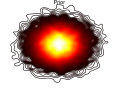
(a) $p(\boldsymbol{z})$

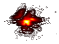
(b) VAE, FC

(c) InfoMax-VAE, FC

(d) VAE, CNN

(e) InfoMax-VAE, CNN

(f) class color

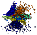
(g) VAE, FC

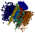
(h) InfoMax-VAE, FC

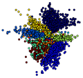
(i) VAE, CNN

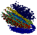
(j) InfoMax-VAE, CNN

Figure 2: Comparing the prior $p(\boldsymbol{z})$ and the aggregated posterior $q_{\phi}(\boldsymbol{z})$ achieved by vanilla VAEs and InfoMax-VAE on MNIST dataset; (a) the prior $p(\boldsymbol{z})$ which is defined to be 2-D standard Gaussian distribution;
(b)(c) aggregated posterior $q_{\phi}(\boldsymbol{z})$ of VAE and InfoMax-VAE with FC NNs;
(d)(e) aggregated posterior $q_{\phi}(\boldsymbol{z})$ of VAE and InfoMax-VAE with CNN;
(f) color of each class;
(g)(h) latent codes of VAE and InfoMax-VAE with FC NN;
(i)(j) latent codes of VAE and InfoMax-VAE with CNN.

To conduct a thorough evaluation of the capability of InfoMax-VAEs in learning representations we employ three different metrics: mutual information, KL divergence, and active units (7). First, to measure the amount of information carried through to latent factors, we utilize the method proposed in belghazi2018mine . We first train autoencoders on a training dataset, and then we provide the observed data and achieved latent representations into another network to estimate the resulting mutual information. A detailed description of this technique can be found in belghazi2018mine . In doing so, we can estimate the mutual information between the input data and latent codes. The KL divergence as in (1) is another metric which represents the divergence between the variational posterior and prior, $\text{KL}(q_{\phi}(\boldsymbol{z}|\boldsymbol{x})||p(\boldsymbol{z}))$.

The active units (AU) metric is another measure to assess latent variable collapse defined in burda2015importance . With this metric, we examine each dimension of the latent code independently from the others, and the believe is that the distribution of a latent dimension changes based on the input data if it keeps useful information. Therefore, it can be expressed as:

$$\text{AU}=\sum_{d=1}^{D}\mathbb{I}\{\text{Cov}_{x}(\mathbb{E}_{q_{\phi}(z_{d}|\boldsymbol{x})}[z_{d}])\geq\epsilon\},$$ (7)

where $z_{d}$ corresponds to the d-th dimension of the latent code $\boldsymbol{z}$, and $\epsilon=0.05$ is a threshold. Also $\mathbb{I}$ is an indicator which is 1 if its argument is true and 0 otherwise. In reliance on these metrics, we compare InfoMax-VAE to other well-known models of VAEs: $\beta$-VAE and Info-VAE. Moreover, we reported the log-likelihood to examine how much the obtained latent codes contribute to retrieve the input.

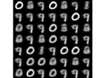
(a) VAE, FC

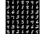
(b) VAE, CNN

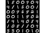
(c) InfoMax-VAE, FC

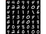
(d) InfoMax-VAE, CNN

Figure 3: Generated samples by vanilla VAEs and InfoMax-VAE trained on MNIST dataset; (a)-(b) samples generated by vanilla VAE using FC and convolutional NNs, (c)-(d) samples of the proposed autoencoder, InfoMax-VAE, using similar architectures.

Table 1: Performance of InfoMax-VAE vs vanilla, $\beta$-, and Info VAEs on MNIST w.r.t log-likelihood-, mutual information, KL divergence on MNIST dataset with FC and convolutional NNs.

Method	$\boldsymbol{z}_{\text{dim}}$	Architecture	log-likelihood	MI	KL	AU
VAE	2	FC	-131.36	2.8882	6.8113	2
$\beta$-VAE	2	FC	-140.26	1.8139	4.4933	2
Info-VAE	2	FC	-197.60	0.3199	9.8007	2
InfoMax-VAE	2	FC	-131.50	3.6180	24.186	2
VAE	20	CNN	-82.96	2.6255	18.3929	10
$\beta$-VAE	20	CNN	-123.34	1.7995	5.2494	13
Info-VAE	20	CNN	-85.12	2.1803	132.5293	20
InfoMax-VAE	20	CNN	-83.36	4.1612	23.4517	20

We summarize the results on MNIST test dataset for networks with FC and Convolutional layers with different size of the latent dimension in Table 1. As the results in Figure 2(i) and also Table 1 show, flexible networks typically result in poor amortized inference. Earlier, we showed that VAEs attempt to compress the aggregated posterior on the center for both FC and convolutional NNs which guarantee the minimization of $\text{KL}(q_{\phi}(\boldsymbol{z}|\boldsymbol{x})||p(\boldsymbol{z}))$. This process severely merges the latent codes regardless of their categories. InfoMax-VAEs mitigate this by assuring maximization of the mutual information between the input and latent codes. Further, InfoMax-VAEs achieve higher mutual information, KL divergence, AUs compared to conventional VAEs and $\beta$-VAEs. For CNNs with 20 latent dimensions, Info-VAEs end up with a large KL divergence which can be observed as its very poor performance in matching the marginalized posterior and prior,see Appendix B for further details. In InfoMax-VAEs, we require that the model encodes sufficient information about observations, which also diligently preserve the KL divergence between $q_{\phi}(\boldsymbol{z})$ and $p(\boldsymbol{z})$ from blowing up. Finally, the samples, $\boldsymbol{x}\sim p_{\theta}(\boldsymbol{x}|\boldsymbol{z})p(\boldsymbol{z})$, generated by the models are presented in Figure 3. All reported metrics are measured on the test dataset.

Table 2: Performance of InfoMax-VAE vs Vanilla, $\beta$, and Info- VAEs on MNIST (Top) and Fashion MNIST (Bottom) w.r.t log-likelihood and AU. The model is fixed at having 20 latent variables. InfoMax-VAE outperforms the others on the aforementioned metrics as varying the complexity of the generative network.

		log-likelihood				AU
Dataset	Layers	VAE	$\beta$-VAE	Info-VAE	InfoMax-VAE	VAE	$\beta$-VAE	Info-VAE	InfoMax-VAE
	2	-86.60	-154.47	-120.61	-103.14	20	19	20	20
MNIST	4	-115.74	-164.64	-130.76	-99.68	20	18	20	20
	10	-153.35	-175.33	-159.23	-146.10	11	14	19	20
	2	-253.87	-265.00	-253.37	-252.17	20	20	20	20
Fashion MNIST	4	-254.44	-291.25	-245.07	-243.46	18	13	20	20
	10	-284.82	-277.54	-266.12	-262.61	9	17	12	20

Table 3: Performance of InfoMax-VAE vs Vanilla, $\beta$, and Info- VAEs on MNIST (Top) and Fashion MNIST (Bottom) w.r.t mutual information and KL divergence. The model is fixed at having 20 latent variables. InfoMax-VAE outperforms the other frameworks on the mentioned metrics as varying the complexity of the generative network.

		Mutual Information				KL Divergence
Dataset	Layers	VAE	$\beta$-VAE	Info-VAE	InfoMax-VAE	VAE	$\beta$-VAE	Info-VAE	InfoMax-VAE
	2	4.32	2.26	3.42	5.03	23.50	5.17	43.25	26.65
MNIST	4	4.37	2.02	2.92	4.60	19.18	3.80	22.59	26.87
	10	3.24	1.35	2.54	4.02	8.25	1.34	18.33	12.99
	2	3.55	2.04	3.36	3.58	16.96	5.57	84.87	18.38
Fashion MNIST	4	3.12	2.12	3.56	3.85	14.28	5.5.	82.09	16.90
	10	3.04	2.53	3.57	3.87	9.64	4.82	43.42	15.72

Table 2 & 3 show the studies on MNIST and Fashion MNIST datasets as the generative networks become richer. In all experiments in this segment, we fix the inference network and set the dimension of latent codes to be 20. Table 2 & 3 suggest that as the generative network becomes more expressive, the latent codes become less reliant on the observations. We can infer this from the evaluated metrics. The InfoMax-VAE, however, helps to mitigate and performs better on all metrics. These results indicate that InfoMax-VAE has a strong inductive bias to keep more information in latent codes even in the presence of complex generative networks. Further, the high KL distance achieved by Info-VAE shows its poor performance in matching $q_{\phi}(\boldsymbol{z})$ and $p(\boldsymbol{z})$, please see Appendix B.

Finally, the samples, $\boldsymbol{x}\sim p_{\theta}(\boldsymbol{x}|\boldsymbol{z})p(\boldsymbol{z})$, generated by the models are presented in Figure 3. We see the results generated by the proposed InfoMax-VAE have more diversity and better quality.

6.2 Generalization

Another evaluation that we performed is the classification task directly on the learned featured of the data. Both the inference and generative networks are fixed after training. Please see Appendix D for details of networks. For this part, we performed evaluation on CIFAR-10 and CIFAR-100 datasets with different dimensions of latent codes. Table 4 shows the results of InfoMax-VAE against vanilla, $\beta$-, and Info- VAEs performed on test dataset. Further, the number of active units are reported for each scenarios. We observe that InfoMax-VAE outperforms other models both in classification and activating all available latent codes. These results suggest that not only the proposed InfoMax-VAE is capable of learning useful and meaningful representations, but it also reveals that the learned features are generalized better than the aforementioned frameworks.

Table 4: Performance of InfoMax-VAE vs Vanilla, $\beta$-, and Info- VAEs on CIFAR-10 and CIFAR-100. The inference and generative networks have the same architecture in all scenarios. InfoMax-VAE outperforms other techniques in both classification and the activation of latent codes.

		Accuracy %				Active Units
Dataset	$\boldsymbol{z}_{dim}$	VAE	$\beta$-VAE	Info-VAE	InfoMax-VAE	VAE	$\beta$-VAE	Info-VAE	InfoMax-VAE
	100	27.52	24.12	31.45	32.55	99	90	93	100
CIFAR-10	200	32.83	25.82	39.05	41.75	187	182	193	200
	500	31.61	24.59	32.74	40.36	490	498	499	500
	100	15.82	11.74	16.57	18.26	99	90	93	100
CIFAR-100	200	14.49	11.46	16.36	17.24	187	182	193	200
	500	10.21	10.59	10.81	16.46	490	498	499	500

6.3 Autoregressive decoder

PixelVAE is like VAE, with one encoder which encodes the data into a posterior distribution over latent codes, and a decoder to retrieve the data. The decoder in PixelVAE, as apposed to VAEs, models $\boldsymbol{x}$ as the product of each dimension $x_{i}$ conditioned an all previous dimensions $x_{j},\forall j=1,2,\cdots,i-1$ and the features $\boldsymbol{z}$:

$$p_{\theta}(\boldsymbol{x}|\boldsymbol{z})=\prod_{i}p_{\theta}(x_{i}|x_{1},x_{2},\cdots,x_{i-1},\boldsymbol{z}),$$

which can be realized by skip connections from input that feed the authorized pixels to the decoder along with the latent codes. In this study, we use a 3-layer ResNet as the inference network, and 12-layer PixelCNN for the generative network. Likewise before, to demonstrate the aggregated posterior we set the dimension of latent codes at 2, and the results for different frameworks are depicted in Figure 4. As mentioned earlier, considering that the authorized ground truth are convoyed to the decoder, vanilla and $\beta$ VAEs fail to notice the inference network properly, and place the confidence in the decoder side of the model. Consequently, achieved latent codes are poor in the quality. Yet, as the results suggest, using the proposed framework, we can generate more meaningful representations than the other frameworks even in the presence of very expressive generative networks.

Also we study the usefulness of learned latent codes quantitatively by evaluating the classification accuracy. In this case, after training, the learned codes are furnished to a network without any hidden layers to examine linear separability of obtained representations. In so doing, we achieve $30.5\%$, $10\%$, $37.98\%$ and $43.35\%$ test accuracy for Pixel VAE, Pixel $\beta$-VAE, Pixel Info-VAE, and Pixel InfoMax-VAE, respectively. As the results suggests, the achieved latent codes by InfoMax-VAE are more representative than those we get from Pixel Info-VAE.

(a) VAE

(b) $\beta$-VAE

(c) Info-VAE

(d) InfoMax-VAE

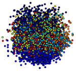
(e) VAE

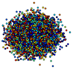
(f) $\beta$-VAE

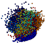
(g) Info-VAE

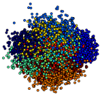
(h) InfoMax-VAE

Figure 4: Comparing the prior $p(\boldsymbol{z})$ and the aggregated posterior $q_{\phi}(\boldsymbol{z})$ of Pixel VAEs, Pixel $\beta$-VAE, and Pixel InfoMax-VAE on binarized MNIST dataset; (a) vanilla Pixel VAE, (b) Pixel $\beta$-VAE, (c) Pixel Info-VAE, (d) Pixel InfoMax-VAE (e)-(h) the latent codes generated by their associated models; latent codes of each categories are painted with different colors. We see that Pixel InfoMax-VAE outperforms three other models as it pushes the learned features of each classes to be assembled in a more meaningful fashion.

6.4 Qualitative Benchmark

Finally, we show the results for VAE and InfoMax-VAE experiments on CelebA, where we set up the dimension of latent code 100. We see in Figure 5 InfoMax-VAE obtains diverse images with much better quality. More results with latent code traversal have been demonstrated in the Appendix E.

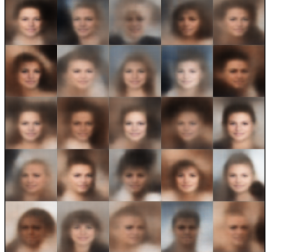
(a) VAE

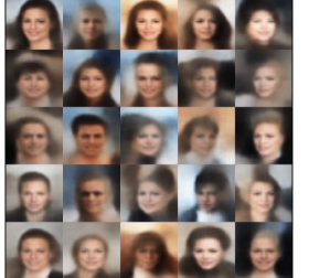
(b) InfoMax-VAE

Figure 5: Generated samples by vanilla VAEs and InfoMax-VAE trained on CelebA dataset. InfoMax-VAE offers a more diverse and better resolution face image when compared to VAE.

7 Conclusion

In this paper we study the problem of representation collapse in VAEs. We find that the conventional objective of VAEs is insufficient towards obtaining general, useful representations. We also determine that rich generative networks discourage the model from learning constructive representations. We propose a new information-based VAE that constrain latent representations so that the amount of information that they store from the observations is maximized, even in the presence of very rich networks. We perform extensive computational experiments and compare our work to other well-known approaches, where the proposed InfoMax-VAE outperforms them based on different metrics.

APPENDIX

A    InfoMax-VAE

In this part, we try to make the intuition behind InfoMax-VAE more explicit. To begin with, the proposed InfoMax-VAE has an objective of the form

$$\begin{split}\max_{\phi,\theta}\mathbb{E}_{q{(\boldsymbol{x})}}[\mathbb{E}_{q_{\phi}(\boldsymbol{z}|\boldsymbol{x})}[\log p_{\theta}(\boldsymbol{x}|\boldsymbol{z})]-&\beta\text{KL}(q_{\phi}(\boldsymbol{z}|\boldsymbol{x})||p(\boldsymbol{z}))]\\ +&\alpha I_{q_{\phi}}(\boldsymbol{x};\boldsymbol{z}).\end{split}$$ (8)

The mutual information induced by the inference network, $I_{q_{\phi}}(\boldsymbol{x};\boldsymbol{z})$, is

$$\begin{split}I_{q_{\phi}}(\boldsymbol{x};\boldsymbol{z})&=\text{KL}(q_{\phi}(\boldsymbol{x},\boldsymbol{z})||q(\boldsymbol{x})q_{\phi}(\boldsymbol{z}))\\ &=\text{KL}(q_{\phi}(\boldsymbol{z}|\boldsymbol{x})||q_{\phi}(\boldsymbol{z}))\\ &=\int q_{\phi}(\boldsymbol{x},\boldsymbol{z})\log\frac{q_{\phi}(\boldsymbol{z}|\boldsymbol{x})}{q_{\phi}(\boldsymbol{z})}d\boldsymbol{x}d\boldsymbol{z},\end{split}$$ (9)

which can be rewritten as

$$\begin{split}I_{q_{\phi}}(\boldsymbol{x};\boldsymbol{z})&=\int q_{\phi}(\boldsymbol{x},\boldsymbol{z})\log\frac{q_{\phi}(\boldsymbol{z}|\boldsymbol{x})}{q_{\phi}(\boldsymbol{z})}d\boldsymbol{x}d\boldsymbol{z}\\ &=\int q_{\phi}(\boldsymbol{x},\boldsymbol{z})[\log\frac{q_{\phi}(\boldsymbol{z}|\boldsymbol{x})}{p(\boldsymbol{z})}+\log\frac{p(\boldsymbol{z})}{q_{\phi}(\boldsymbol{z})}]d\boldsymbol{x}d\boldsymbol{z}\\ &=\int q_{\phi}(\boldsymbol{x},\boldsymbol{z})\log\frac{q_{\phi}(\boldsymbol{z}|\boldsymbol{x})}{p(\boldsymbol{z})}d\boldsymbol{x}d\boldsymbol{z}-\int q_{\phi}(\boldsymbol{z})\log\frac{q_{\phi}(\boldsymbol{z})}{p(\boldsymbol{z})}d\boldsymbol{z}\\ &=\text{KL}(q_{\phi}(\boldsymbol{z}|\boldsymbol{x})||p({\boldsymbol{z}}))-\text{KL}(q_{\phi}(\boldsymbol{z})||p({\boldsymbol{z}})).\end{split}$$ (10)

By replacing (10) into (3) we have

$$\begin{split}\max_{\phi,\theta}\mathbb{E}_{q{(\boldsymbol{x})}}[\mathbb{E}_{q_{\phi}(\boldsymbol{z}|\boldsymbol{x})}[\log p_{\theta}(\boldsymbol{x}|\boldsymbol{z})]+&(\alpha-\beta)\text{KL}(q_{\phi}(\boldsymbol{z}|\boldsymbol{x})||p(\boldsymbol{z}))\\ -&\alpha\text{KL}(q_{\phi}(\boldsymbol{z})||p({\boldsymbol{z}})).\end{split}$$ (11)

Now if $\alpha>\beta$, instead of minimizing the KL divergence between the posterior and prior, $\text{KL}(q_{\phi}(\boldsymbol{z}|\boldsymbol{x})||p(\boldsymbol{z}))$, InfoMax-VAE seeks for the solution that maximize this distance. The objective, however, is regularized by the KL divergence between the marginal of the posterior $q_{\phi}(\boldsymbol{z})$ and the prior $p(\boldsymbol{z})$, $\text{KL}(q_{\phi}(\boldsymbol{z})||p({\boldsymbol{z}}))$. Indeed, in VAE with the minimization of $\text{KL}(q_{\phi}(\boldsymbol{z}|\boldsymbol{x})||p(\boldsymbol{z}))$, it pushes the model to encode a handful of input data $\boldsymbol{x}$ into limited and close points in the feature space $\boldsymbol{z}$. In InfoMax-VAE, as opposed to VAE, the model seeks to encode the input data to distinct points in the feature space to be more repenstative for their input. However, now we have more sensible regularizer $\text{KL}(q_{\phi}(\boldsymbol{z})||p({\boldsymbol{z}}))$ which is crucial to the model.

   InfoMax-VAE vs. InfoVAE

I. Objective: Info-VAEs proposed to optimize (11) to circumvent from calculating the mutual information. The approach in this paper (InfoMax-VAE), however, directly optimize (8) instead. Indeed, InfoMax-VAE estimates the mutual information by means of an MLP and is different in the algorithm. In so doing, while InfoVAE tries to minimize distance between $q_{\phi}(\boldsymbol{z})$ and $p(\boldsymbol{z})$, our method tries to maximize the distance between $q_{\phi}(\boldsymbol{x},\boldsymbol{z})$ and $q(\boldsymbol{x})q_{\phi}(\boldsymbol{z})$ to ensure the dependency between the input and latent codes. Moreover, we also examine different distances between them. See Figure 1 here.

II. Information preference: More important than the objectives, InfoVAE is limited to $\alpha\leq 1$ since they circumvent the mutual information; otherwise, the term $\text{KL}(q_{\phi}(\boldsymbol{z}|\boldsymbol{x})||p(\boldsymbol{z}))$ blows up in the first iteration since the encoder immediately learns with $\sigma_{z|x}=0$ the InfoVAE’s objective becomes infinity (as ($\textbf{KL}(q_{\phi}(\boldsymbol{z}|\boldsymbol{x})||p(\boldsymbol{z}))\rightarrow\infty$). Note that the Info-VAE’s obejctive is: $\max_{\phi,\theta}\mathbb{E}_{q{(\boldsymbol{x})}}[\mathbb{E}_{q_{\phi}(\boldsymbol{z}|\boldsymbol{x})}[\log p_{\theta}(\boldsymbol{x}|\boldsymbol{z})]-(1-\alpha)\text{KL}(q_{\phi}(\boldsymbol{z}|\boldsymbol{x})||p(\boldsymbol{z}))-(\alpha+\lambda-1)\text{KL}(q_{\phi}(\boldsymbol{z})||p({\boldsymbol{z}}))$ . Therefore, the amount of useful information in latent variables for InfoVAE is limited because of the restrictions imposed by $(1-\alpha)\text{KL}(q_{\phi}(\boldsymbol{z}|\boldsymbol{x})||p(\boldsymbol{z}))$. However, our proposed InfoMax does not require $\alpha<1$. Note that $\alpha$ plays a critical role as it determines the information preference in VAEs. Also, we believe this flexibility in the choice of $\alpha>1$ is the primary reason why InfoMax-VAE outperforms Info-VAE in all models and datasets, as we enable the resulting autoencoder to uncover more information-rich latent codes compared to Info-VAE.

B    $\text{KL}(q_{\phi}(\boldsymbol{z}|\boldsymbol{x})||p(\boldsymbol{z}))$ and $I_{q_{\phi}}(\boldsymbol{x};\boldsymbol{z})$

In this section, we explore the interpretation of very large $\text{KL}(q_{\phi}(\boldsymbol{z}|\boldsymbol{x})||p(\boldsymbol{z}))$. As showed earlier, $I_{q_{\phi}}(\boldsymbol{x};\boldsymbol{z})=\text{KL}(q_{\phi}(\boldsymbol{z}|\boldsymbol{x})||p({\boldsymbol{z}}))-\text{KL}(q_{\phi}(\boldsymbol{z})||p({\boldsymbol{z}}))$. It is easy to show that $I_{q_{\phi}}(\boldsymbol{x};\boldsymbol{z})\leq\log N$, where $N$ is the total number of input data, which, for example, is $11.002$ for MNIST dataset. That, therefore, means very large $\text{KL}(q_{\phi}(\boldsymbol{z}|\boldsymbol{x})||p(\boldsymbol{z}))$ should have very large $\text{KL}(q_{\phi}(\boldsymbol{z})||p(\boldsymbol{z}))$ to compensate that for $I_{q_{\phi}}(\boldsymbol{x};\boldsymbol{z})$. If this scenario happens, very large $\text{KL}(q_{\phi}(\boldsymbol{z})||p(\boldsymbol{z}))$ can be interpreted as the model’s failure in matching the marginalized posterior and the prior. So, for Info-VAE we have $\text{KL}(q_{\phi}(\boldsymbol{z}|\boldsymbol{x})||p(\boldsymbol{z}))=132.52$ and $\text{KL}(q_{\phi}(\boldsymbol{z})||p(\boldsymbol{z}))\geq 121.51$ (see Table 1-3), which essentially means a poor performance in matching to the prior and also collapse in generalization.

C    Other Divergences

As it is stated in the main manuscript, we can easily replace the $f$-divergence with other distances or dual representations. Here, for example, we substitute Donsker-Varadhan dual representation, where we got the objective of form

$$\begin{split}\max_{\phi,\theta,t}\mathbb{E}_{q{(\boldsymbol{x})}}[&\mathbb{E}_{q_{\phi}(\boldsymbol{z}|\boldsymbol{x})}[\log p_{\theta}(\boldsymbol{x}|\boldsymbol{z})]-\text{KL}(q_{\phi}(\boldsymbol{z}|\boldsymbol{x})||p(\boldsymbol{z}))]\\ +&\alpha(\mathbb{E}_{q_{\phi}(\boldsymbol{x},\boldsymbol{z})}[t(\boldsymbol{x},\boldsymbol{z})]-\log\mathbb{E}_{q(\boldsymbol{x})q_{\phi}(\boldsymbol{z})}[\exp(t(\boldsymbol{x},\boldsymbol{z}))]).\end{split}$$ (12)

Despite the difference, we can still employ Algorithm 1 to optimize the networks. But the output layer of the MLP has to be modified, please see [3]. In Figure 6, we study the proposed model for different divergence terms (or different dual representations) $D(q_{\phi}(\boldsymbol{x},\boldsymbol{z})||q_{\phi}(\boldsymbol{x})q_{\phi}(\boldsymbol{z}))$. We mostly used $f$-divergence dual representations, however, we also investigate another dual representation for the KL divergence, Donsker-Varadhan representation. To compare different divergences meterics against each other, we reported the reconstruction errors at each training iteration, see Figure 6 on MNIST dataset. We have seen the same outputs for the other datasets as well.

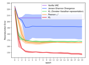
(a)

Figure 6: Reconstruction error for different divergence term. We see that the best results are achieved for the KL divergence with f-dual representation.

D    Architectures and Settings

In all experiments we set the prior to be standard normal distribution, $p(\boldsymbol{z})\sim\mathcal{N}(0,1)$. And also we used Adam optimizer with learning rate 1e-3 for the inference and generative networks, and 1e-4 for the network estimates the $f$-divergence. Tables 5-8 show the architectures of networks.

Table 5: Encoder and decoder architecture for MNIST & Fashion MNIST. $\alpha=10,\beta=1$.

Encoder	Decoder
Input 28$\times$28 images	Input $\boldsymbol{z}$
FC 4$\times$1000 LeakyReLU(0.2)	FC 4$\times$1000 LeakyReLU(0.2)
FC 2$\times\boldsymbol{z}_{dim}$	FC $28\times 28$ Sigmoid
Input 28$\times$28 images	Input $\boldsymbol{z}$, 1$\times$1 conv, 118 ReLU, stride 1
4$\times$4 conv, 28 ReLU, stride 2	4$\times$4 upconv, 118 ReLU, stride 2
4$\times$4 conv, 28 ReLU, stride 2	4$\times$4 upconv, 56 ReLU, stride 2
4$\times$4 conv, 56 ReLU, stride 2	4$\times$4 upconv, 28 ReLU, stride 2
4$\times$4 conv, 118 ReLU, stride 2	4$\times$4 upconv, 28 ReLU, stride 2
4$\times$4 conv, 2$\times\boldsymbol{z}_{dim}$, stride 1	4$\times$4 upconv, 1 Sigmoid, stride 2

Table 6: Encoder and decoder architecture for CIFAR-10 & CIFAR-100. $\alpha=10,\beta=0.1$.

Encoder	Decoder
Input 32$\times$32 RGB images	Input $\boldsymbol{z}$, 1$\times$1 conv, 128 ReLU, stride 1
4$\times$4 conv, 32 ReLU, stride 2	4$\times$4 upconv, 128 ReLU, stride 2
4$\times$4 conv, 32 ReLU, stride 2	4$\times$4 upconv, 64 ReLU, stride 2
4$\times$4 conv, 64 ReLU, stride 2	4$\times$4 upconv, 64 ReLU, stride 2
4$\times$4 conv, 128 ReLU, stride 2	4$\times$4 upconv, 32 ReLU, stride 2
4$\times$4 conv, 2$\times\boldsymbol{z}_{dim}$, stride 1	4$\times$4 upconv, 3 Sigmoid, stride 2

Table 7: Classifier Architecture for CIFAR-10 and CIFAR-100

Encoder
Input $\boldsymbol{z}$ learned features
FC $1000$ ReLU
FC $500$ ReLU
FC $100$ ReLU
FC $10$ (CIFAR-10) OR $100$ (CIFAR-100)
Softmax()

Table 8: Encoder and decoder architecture for CelebA. $\alpha=10,\beta=1$, $\boldsymbol{z}_{\text{dim}}=100$.

Encoder	Decoder
Input 64$\times$64 RGB images	Input $\boldsymbol{z}$, 1$\times$1 conv, 256 ReLU, stride 1
4$\times$4 conv, 32 LeakyReLU(0.2), stride 2	4$\times$4 upconv, 128 ReLU, stride 2
4$\times$4 conv, 64 LeakyReLU(0.2), stride 2	4$\times$4 upconv, 128 ReLU, stride 2
4$\times$4 conv, 128 LeakyReLU(0.2), stride 2	4$\times$4 upconv, 64 ReLU, stride 2
4$\times$4 conv, 256 LeakyReLU(0.2), stride 2	4$\times$4 upconv, 32 ReLU, stride 2
4$\times$4 conv, 2$\times\boldsymbol{z}_{dim}$, stride 1	4$\times$4 upconv, 32 ReLU, stride 2
	4$\times$4 upconv, 3 Sigmoid, stride 2

E    Hyperparameters

We find that batch size does not prove to be crucial for the insights underlying our work. For typical choices like 64, 100, or more, our approach works well. Specifically, our methodology works as long as the batch size is large enough to ensure that permuting the latent variables assigns the to different input data. Therefore, small batch size such as 10 or lower are not suitable. Typical choices from literature such as 64, 100 or more work well, and there is not a significant impact on performance.

Behavior of InfoMax-VAE in terms of $\alpha$ and $\beta$: By increasing $\alpha$, the MI coefficient, we enable the model to uncover distinct latent variables for each input to ensure the maximization of $I_{q_{\phi}}(\boldsymbol{x},\boldsymbol{z})$. However, very large $\alpha$ will cause the posterior distribution not to adequately match the prior. For $\beta$, note that $\beta*KL(q(z|x)|p(z))$ acts as a regularizer, encouraging models to discover latent variables which are irrelevant to the input. Through several experiments, we conclude that $\alpha=10-20$ and $\beta=1$ work better based on different metrics, AU, MI, accuracy, and KL. See Figure 7 and 8. 2) $\epsilon$: As our experiments show, as in [28], the distribution of $COV(\mathbb{E}_{q}(\boldsymbol{z}))$ is widely separated bimodal, therefore, epsilon is often opted in $[0.01,0.1]$.

(a) $\alpha=1,\beta=1$

(b) $\alpha=2,\beta=1$

(c) $\alpha=10,\beta=1$

(d) $\alpha=50,\beta=1$

(e) $\alpha=100,\beta=1$

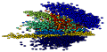
(f) $\alpha=1,\beta=1$

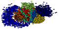
(g) $\alpha=2,\beta=1$

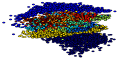
(h) $\alpha=10,\beta=1$

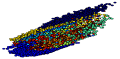
(i) $\alpha=50,\beta=1$

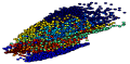
(j) $\alpha=100,\beta=1$

Figure 7: The aggregated posterior $q_{\phi}(\boldsymbol{z})$ (first row) with their associated latent codes (second row). Varying $\alpha$ with fixed $\beta$.

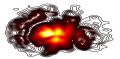
(a) $\alpha=1,\beta=1$

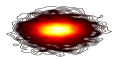
(b) $\alpha=1,\beta=2$

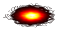
(c) $\alpha=1,\beta=10$

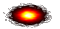
(d) $\alpha=1,\beta=50$

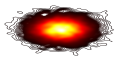
(e) $\alpha=1,\beta=100$

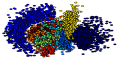
(f) $\alpha=1,\beta=1$

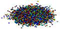
(g) $\alpha=1,\beta=2$

(h) $\alpha=1,\beta=10$

(i) $\alpha=1,\beta=50$

(j) $\alpha=1,\beta=100$

Figure 8: The aggregated posterior $q_{\phi}(\boldsymbol{z})$ (first row) with their associated latent codes (second row). Varying $\beta$ with fixed $\alpha$.

F    Latent Traversals

We show generated faces with InfoMax-VAE in Figure 9. For each image, we fix $90\%$ of latent codes and change the rest from -4 to 4.

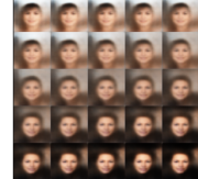
(a)

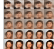
(b)

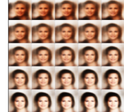
(c)

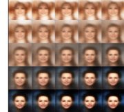
(d)

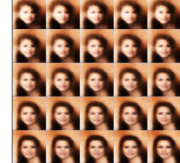
(e)

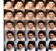
(f)

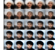
(g)

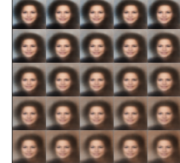
(h)

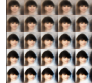
(i)

Figure 9: Qualitative results for CelebA dataset. In each case, $10\%$ of the latent codes are varying from -4 to 4, and the rest of them are fixed.

References

- [1] Yunchen Pu, Win Yuan, Andrew Stevens, Chunyuan Li, and Lawrence Carin. A deep generative deconvolutional image model. In Artificial Intelligence and Statistics, pages 741–750, 2016.
- [2] Alec Radford, Luke Metz, and Soumith Chintala. Unsupervised representation learning with deep convolutional generative adversarial networks. arXiv preprint arXiv:1511.06434, 2015.
- [3] Sebastian Nowozin, Botond Cseke, and Ryota Tomioka. f-gan: Training generative neural samplers using variational divergence minimization. In Advances in Neural Information Processing Systems 29, pages 271–279. 2016.
- [4] R Devon Hjelm, Alex Fedorov, Samuel Lavoie-Marchildon, Karan Grewal, Adam Trischler, and Yoshua Bengio. Learning deep representations by mutual information estimation and maximization. arXiv preprint arXiv:1808.06670, 2018.
- [5] Diederik P Kingma and Max Welling. Auto-encoding variational bayes. arXiv preprint arXiv:1312.6114, 2013.
- [6] Samuel R Bowman, Luke Vilnis, Oriol Vinyals, Andrew M Dai, Rafal Jozefowicz, and Samy Bengio. Generating sentences from a continuous space. arXiv preprint arXiv:1511.06349, 2015.
- [7] Yunchen Pu, Zhe Gan, Ricardo Henao, Xin Yuan, Chunyuan Li, Andrew Stevens, and Lawrence Carin. Variational autoencoder for deep learning of images, labels and captions. In Advances in neural information processing systems, pages 2352–2360, 2016.
- [8] Jiacheng Xu and Greg Durrett. Spherical latent spaces for stable variational autoencoders. arXiv preprint arXiv:1808.10805, 2018.
- [9] Michael Tschannen, Olivier Bachem, and Mario Lucic. Recent advances in autoencoder-based representation learning. arXiv preprint arXiv:1812.05069, 2018.
- [10] Alexander A Alemi, Ben Poole, Ian Fischer, Joshua V Dillon, Rif A Saurous, and Kevin Murphy. Fixing a broken elbo. arXiv preprint arXiv:1711.00464, 2017.
- [11] Adji B. Dieng, Yoon Kim, Alexander M. Rush, and David M. Blei. Avoiding latent variable collapse with generative skip models. In Proceedings of Machine Learning Research, volume 89, pages 2397–2405. PMLR, 16–18 Apr 2019.
- [12] Danilo Jimenez Rezende, Shakir Mohamed, and Daan Wierstra. Stochastic backpropagation and approximate inference in deep generative models. arXiv preprint arXiv:1401.4082, 2014.
- [13] Alireza Makhzani, Jonathon Shlens, Navdeep Jaitly, Ian Goodfellow, and Brendan Frey. Adversarial autoencoders. arXiv preprint arXiv:1511.05644, 2015.
- [14] Jake Zhao, Yoon Kim, Kelly Zhang, Alexander M Rush, and Yann LeCun. Adversarially regularized autoencoders. arXiv preprint arXiv:1706.04223, 2017.
- [15] Ian Goodfellow, Jean Pouget-Abadie, Mehdi Mirza, Bing Xu, David Warde-Farley, Sherjil Ozair, Aaron Courville, and Yoshua Bengio. Generative adversarial nets. In Advances in neural information processing systems, pages 2672–2680, 2014.
- [16] Irina Higgins, Loic Matthey, Arka Pal, Christopher Burgess, Xavier Glorot, Matthew Botvinick, Shakir Mohamed, and Alexander Lerchner. beta-vae: Learning basic visual concepts with a constrained variational framework. ICLR, 2(5):6, 2017.
- [17] Xi Chen, Diederik P Kingma, Tim Salimans, Yan Duan, Prafulla Dhariwal, John Schulman, Ilya Sutskever, and Pieter Abbeel. Variational lossy autoencoder. arXiv preprint arXiv:1611.02731, 2016.
- [18] Shengjia Zhao, Jiaming Song, and Stefano Ermon. Towards deeper understanding of variational autoencoding models. arXiv preprint arXiv:1702.08658, 2017.
- [19] Zichao Yang, Zhiting Hu, Ruslan Salakhutdinov, and Taylor Berg-Kirkpatrick. Improved variational autoencoders for text modeling using dilated convolutions. In Proceedings of the 34th International Conference on Machine Learning, volume 70, pages 3881–3890. PMLR, 06–11 Aug 2017.
- [20] Aaron van den Oord, Oriol Vinyals, and koray kavukcuoglu. Neural discrete representation learning. In Advances in Neural Information Processing Systems 30, pages 6306–6315. 2017.
- [21] Chunyuan Li, Hao Liu, Changyou Chen, Yuchen Pu, Liqun Chen, Ricardo Henao, and Lawrence Carin. Alice: Towards understanding adversarial learning for joint distribution matching. In Advances in Neural Information Processing Systems 30, pages 5495–5503. 2017.
- [22] Yuchen Pu, Weiyao Wang, Ricardo Henao, Liqun Chen, Zhe Gan, Chunyuan Li, and Lawrence Carin. Adversarial symmetric variational autoencoder. In Advances in Neural Information Processing Systems 30, pages 4330–4339. Curran Associates, Inc., 2017.
- [23] Matthew D Hoffman and Matthew J Johnson. Elbo surgery: yet another way to carve up the variational evidence lower bound. In Workshop in Advances in Approximate Bayesian Inference, NIPS, volume 1, 2016.
- [24] Hyunjik Kim and Andriy Mnih. Disentangling by factorising. In Proceedings of the 35th International Conference on Machine Learning, volume 80 of Proceedings of Machine Learning Research, pages 2649–2658, Stockholmsmässan, Stockholm Sweden, 10–15 Jul 2018. PMLR.
- [25] Shengjia Zhao, Jiaming Song, and Stefano Ermon. Infovae: Balancing learning and inference in variational autoencoders. In Proceedings of the AAAI Conference on Artificial Intelligence, volume 33, pages 5885–5892, 2019.
- [26] Miguel A Arcones and Evarist Gine. On the bootstrap of u and v statistics. The Annals of Statistics, pages 655–674, 1992.
- [27] Mohamed Ishmael Belghazi, Aristide Baratin, Sai Rajeswar, Sherjil Ozair, Yoshua Bengio, Aaron Courville, and R Devon Hjelm. Mine: mutual information neural estimation. arXiv preprint arXiv:1801.04062, 2018.
- [28] Yuri Burda, Roger Grosse, and Ruslan Salakhutdinov. Importance weighted autoencoders. arXiv preprint arXiv:1509.00519, 2015.