Effects of Postselected von Neumann Measurement on the Properties of Single-Mode Radiation Fields

Abstract

Postselected von Neumann measurement characterized by postselection and weak value has been found potential applications in quantum metrology and solved plenty of fundamental problems in quantum theory. As an application of this new measurement technique in quantum optics and quantum information processing, its effects on the features of single-mode radiation fields such as coherent state, squeezed vacuum state and Schrödinger cat sate are investigated by considering full-order effects of unitary evolution. The results show that the conditional probabilities of finding photons, second-order correlation functions, $Q_{m}$-factors and squeezing effects of those states after postselected measurement significantly changed compared with the corresponding initial pointer states.

I Introduction

Most researches in von Neumann type quantum measurement in recent years has focused on postseleceted weak measurement with sufficiently weak coupling between the measured system and pointer since it is useful to study the nature of the quantum world. This kind of postsselected weak measurement theory is originally proposed by Aharonov, Albert, and Vaidman in 1988 (Aharonov et al., 1988), and considered as a generalized version of standard von-Neumann type measurement (von Neumann J, 1955). The result of weak coupling postselected weak measurement is called “weak value”, and generally is a complex number. One of the special feature of the “weak value ” is that it can take the values, which lie beyond the normal eigenvalue range of corresponding observable, and this effect is very clear if the pre- and post-selected state almost orthogonal. This feature of “weak value ” is called signal amplification property of postselected weak measurement and its first weak signal amplification property experimentally demonstrated in 1991 (Ritchie et al., 1991). After that, it has been widely used and elucidated tremendous fundamental problems in quantum mechanics. For details about the weak measurement and its applications in signal amplification processes, we refer the reader to the recent overview of the field (Kofman et al., 2012; Dressel et al., 2014). As we mentioned earlier, in postselected weak measurement the interaction strength is weak, and it is enough to consider up to the first order evolution of unitary operator for the whole measurement processes. However, if we want to connect the weak and strong measurement, check to clear the measurement feedback of postselected weak measurement and analyze experimental results obtained in nonideal measurements, the full order evolution of unitary operator is needed (Aharonov and Botero, 2005; Di Lorenzo and Egues, 2008; Pan and Matzkin, 2012), we call this kind of measurement is postselected von-Neumann measurement. We know that in some quantum metrology problems the precision of the measurement depends on measuring devices and require to optimize the pointer states. The merits of postselected von-Neumann measurement can be seen in pointer optimization schemes.

Recently, the state optimization problem in postselected von-Neumann measurement have been presented widely, such as taking the Gaussian states (Kofman et al., 2012; Nakamura et al., 2012), Hermite-Gaussian or Laguerre-Gaussian states, and non-classical states (Turek et al., 2015a; de Lima Bernardo et al., 2014a). The advantages of non-classical pointer states in increasing postselected measurement precision have been examined in recent studies (Turek et al., 2015b, a; Pang and Brun, 2015). Furthermore, in Ref. (Turek and Yusufu, 2018), the authors studied the effects of postselected measurement characterized by modular value (Kedem and Vaidman, 2010) to show the properties of semi-classical and non-classical pointer states considering the coherent, coherent squeezed, and Schrodinger cat state as a pointer. Since in their scheme the pointer operator is a projection operator onto one of the states of the basis of the pointer’s Hilbert space and interaction strength only has taken one definite value, it can’t completely describe the effects of postselected measurement on the properties of the radiation field. However, to the knowledge of the author, the issue related to the study of the effects of postselected von-Neumann measurement considering all interaction strengths to the inherent properties such as photon distribution, photon statistics, and squeezing effects of radiation field have not been handled and need to be investigated.

Furthermore, the above mentioned properties of quantum radiation fields have many useful technological applications in quantum optics and quantum information processing such as single photon generation and detection (Buller and Collins, 2010), gravitational wave detection (Khalili et al., 2009; Grote et al., 2016), quantum teleportation, (Braunstein and Kimble, 1998; Milburn and Braunstein, 1999; Jeong et al., 2001; van Enk and Hirota, 2001), quantum computation (Ralph et al., 2003), generation and manipulation of atom-light entanglement (Muschik et al., 2006; Li et al., 2013; Hacker et al., 2019), and precision measurements (Munro et al., 2002) etc. We know that the realization of these processes depends on the optimization of the related input quantum states such as coherent state (Glauber, 1963), squeezed state (Carranza and Gerry, 2012; Andersen et al., 2016) and Schrödinger cat state (Monroe et al., 1996; Ourjoumtsev et al., 2007; Haroche, 2013). As introduced in previous part, the postselected weak measurement technique have more advantageous on signal optimization problem (Starling et al., 2009) and precision metrology (Hosten and Kwiat, 2008; Dixon et al., 2009; Zhou et al., 2013; Starling et al., 2010; Magaña Loaiza et al., 2014; Pfeifer and Fischer, 2011; de Lima Bernardo et al., 2014b; Viza et al., 2013; Egan and Stone, 2012) than traditional measurement theory. Thus, the investigation of the effects of postselected von-Neumann measurement on the statistical and squeezing properties of radiation fields is worth to study to optimize the related quantum states to provide more effective methods for the implementation of the above mentioned technological processes.

In this paper, motivated by the above listed problems, we describe and examine the effects of postselected von-Neumann measurement characterized by postselection and weak value on the properties of single-mode radiation fields. In order to achieve our goal, we choose the three typical states such as coherent state, squeezed vacuum state, and Schrödinger cat state as pointers and consider their polarization degree of freedom as measured system, respectively. By taking full-order evolution of the unitary operator of our system, we separately study the photon distributions, statistical properties and squeezing effects of radiation fields and compare that with the initial state cases. To give more details about the effects of postselected von-Neumann measurement on radiation fields, we plot more figures by considering all parameters which related to the properties of those radiation fields, respectively. This study shows that the postselected measurement changes the properties of single-mode radiation fields dramatically for strong and weak measurement regimes with specific weak values. Especially the photon statistics and squeezing effect of coherent pointer state is too sensitive for the postselected von-Neumann measurement processes.

This paper is organized as follows: In Section. II, we describe the model of our theory by brief reviewing the postselected von-Neumann measurement and outline the tasks we want to investigate. In Section. III, we separately calculate exact analytical expressions of photon distribution, second-order correlation function, Mandel factor and squeezing parameter of those three-pointers by taking into account the full-order evaluation of unitary operator under final states which given after postselected measurement finished and present our main results, respectively. Finally, we summarize our findings of this study in Sec. IV.

II Model Setup

To build up our model, we begin to review some basic concepts of the von-Neumann measurement theory. The standard measurement consists of three elements; measured system, pointer ( measuring device or meter) and environment, which induce the interaction between system and pointer. The description of the measurement process can be written in terms of Hamiltonian, and the total Hamiltonian of a measurement composed of three parts (Aharonov and Rohrlich, 2005)

$$H=H_{s}+H_{p(m)}+H_{int},$$ (1)

where $H_{s}$ and $H_{p(m)}$ represents the Hamiltonian of measured system and measuring device, respectively, and $H_{int}$ is the interaction Hamiltonian between measured system and pointer. By considering the measurement efficiency and accuracy, in standard quantum measurement theory the interaction time between system and meter required to be too short so that the $H_{s}$ and $H_{p(m)}$ doesn’t affect the final readout of the measurement result. Thus, in general, a measurement can only be described by the interaction part $H_{int}$ of the total Hamiltonian, and it is taken to the standard von Neumann Hamiltonian as (von Neumann J, 1955)

$$H_{int}=g(t)\hat{A}\hat{P},\ \ \ \ \int_{t_{0}}^{t}g(t)dt=g\text{$\delta(t-t_{0})$.}$$ (2)

Here, $\hat{A}$ represents the Hermitian operator corresponding to the observable of the system that we want to measure with $\hat{A}|\phi_{n}\rangle=a_{n}|\phi_{n}\rangle$, and $\hat{P}$ is the conjugate momentum operator to the position operator $\hat{X}$ of the pointer, i.e., $[\hat{X},\hat{P}]=i\hat{I}$. The coupling $g(t)$ is a nonzero function in a finite interaction time interval $t-t_{0}$.

One can express the position $\hat{X}$ and momentum operator $\hat{P}$ of the pointer by using the annihilation $\hat{a}$ and creation operator $\hat{a}^{\dagger}$ (satisfying $[\hat{a},\hat{a}^{\dagger}]=1$) as (Gerry and Knight, 2005)

$$\hat{X} = \sigma(\hat{a}^{\dagger}+\hat{a}),$$ (3)

$$\hat{P} = \frac{i}{2\sigma}(\hat{a}^{\dagger}-\hat{a}),$$ (4)

where $\sigma$ is the width of the beam. The Hamiltonian $H_{int}$ can be rewritten in terms of $a$ and $a^{\dagger}$ as $H_{int}=\frac{ig(t)}{2\sigma}\hat{A}(a^{\dagger}-a)$. If the Hermitian operator $\hat{A}$ satisfies the property $\hat{A}^{2}=\hat{I}$, then the unitary evolution operator $e^{-i\int_{t_{0}}^{t}H_{int}d\tau}$ of our coupling system is given by

$$e^{-ig\hat{A}\otimes\hat{P}}=\frac{1}{2}(\hat{I}+\hat{A})\otimes D(\frac{s}{2})+\frac{1}{2}(\hat{I}-\hat{A})\otimes D(-\frac{s}{2}),$$ (5)

where $s$ is defined by $s:\equiv g/\sigma$, and $D\left(\frac{s}{2}\right)$ is a displacement operator and its expression can be written as $D(\frac{s}{2})=e^{\frac{s}{2}(\hat{a}^{\dagger}-\hat{a})}$. We have to note that $s$ characterizes the measurement strength, and $s\ll 1$$(s>1)$ corresponds to weak (strong) measurement regimes, respectively.

Assume that the system initially prepared in the state $|\psi_{i}\rangle$ and the initial pointer state is $|\phi\rangle$, then after interaction we project the state $e^{-i\int_{t_{0}}^{t}H_{int}d\tau}|\psi_{i}\rangle|\phi\rangle$ onto the postselected system state $|\psi_{f}\rangle$, we can obtain the final state of the pointer. Furthermore, the normalized final state of the pointer can be written as

$$|\Phi\rangle=\mathcal{N\!}\left[\!\frac{1}{2}(\hat{I}\!+\!\langle A\rangle{}_{w}\!)\!\otimes\!D(\frac{s}{2})\!+\!\frac{1}{2}(\hat{I}\!-\!\langle A\rangle{}_{w})\!\otimes\!D(-\frac{s}{2})\!\right]\!\!|\phi\rangle.$$ (6)

Here, $\mathcal{N}$ is the normalization coefficient of $|\Phi\rangle$, and

$$\langle A\rangle{}_{w}=\frac{\langle\psi_{f}|\hat{A}|\psi_{i}\rangle}{\langle\psi_{f}|\psi_{i}\rangle},$$ (7)

is called the weak value of Hermitian operator $\hat{A}$. From Eq. (7), we know that when the preselected state $|\psi_{i}\rangle$ and the postselected state $|\psi_{f}\rangle$ of the system are almost orthogonal, the absolute value of the weak value can be arbitrarily large and can beyond the eigenvalue region of observable $A$. This feature leads to weak value amplification of weak signals, and solved a lot of important problems in physics.

In this study, we take the transverse spatial degree of freedom of single-mode radiation field as pointer and its polarization degree of freedom as a measured system. We suppose that the operator to be observed is the spin $x$ component of a spin- $1/2$ particle, i.e.,

$$A=\sigma_{x}=|\uparrow_{z}\rangle\langle\downarrow_{z}|+|\downarrow_{z}\rangle\langle\uparrow_{z}|,$$ (8)

where $|\uparrow_{z}\rangle$ and $\langle\downarrow_{z}|$ are eigenstates of the $z$-component of spin, $\sigma_{z}$, with the corresponding eigenvalues $1$ and $-1$, respectively. We assume that the pre- and post-selected states of measured system are

$$|\psi_{i}\rangle=\cos\frac{\theta}{2}|\uparrow_{z}\rangle+e^{i\varphi}\sin\frac{\theta}{2}|\downarrow_{z}\rangle,$$ (9)

and

$$|\psi_{f}\rangle=|\uparrow_{z}\rangle,$$ (10)

respectively, and the corresponding weak value, Eq. (7) reads

$$\langle\sigma_{x}\rangle_{w}=e^{i\varphi}\tan\frac{\theta}{2},$$ (11)

where $\theta\in[0,\pi]$ and $\varphi\in[0,2\pi)$. Here, in our system, the post-selection probability is $P_{s}=\cos^{2}\frac{\theta}{2}$. Note that throughout the rest of this study we will use this weak value for our purposes.

Furthermore, we take the initial pointer state $|\phi\rangle$ as a coherent state, squeezed vacuum state and Schrodinger cat state to study the effects of postselected measurement on the properties of those pointers, respectively. To achieve our goal:

1. we study the conditional probability of finding $n$ photons after postselected measurement. For the state $|\Phi\rangle$, the conditional probability of finding $n$ photons can be calculated by

$$P_{post}(n)=|\langle n|\Phi\rangle|^{2},$$ (12)

and we compare it with the probability $P(n)=|\langle n|\phi\rangle|^{2}$ of initial pointer state $|\phi\rangle$.

2.we investigate the second-order correlation function $g^{(2)}(0)$ and Mandel factor $Q_{m}$ for the $|\Phi\rangle$ state. The second-order correlation function of a single-mode radiation field is defined as

$$g^{(2)}(0) =\frac{\langle a^{\dagger}a^{\dagger}aa\rangle}{\langle a^{\dagger}a\rangle^{2}},$$ (13)

and the Mandel factor $Q_{m}$of the radiation field can be expressed in terms of $g^{(2)}(0)$ as

$$Q_{m}=\langle n\rangle\left[g^{(2)}(0)-1\right]$$ (14)

If $0\leq g^{(2)}(0)<1$ and $-1\leq Q_{m}<0$ simultaneously, the corresponding radiation field have sub-Poissonian statistics and more nonclassical. We have mention that the quantity $Q_{m}$ can never be smaller than -1 for any radiation field, and negative $Q_{m}$ values which equivalent to sub-poissonian statistics, cannot be produced by any classical field (Mandel, 1979).

3.we check the squeezing parameter of single-mode radiation field for the $|\Phi\rangle$ state. The squeezing parameter of the single-mode radiation field reads as (Agarwal, 2013)

$$S_{\phi}=\langle:X_{\phi}^{2}:\rangle-\langle X_{\phi}\rangle^{2}$$ (15)

where

$$X_{\phi}=\frac{1}{\sqrt{2}}\left(ae^{-i\phi}+a^{\dagger}e^{i\phi}\right),\ \ \ [X_{\phi},X_{\phi+\frac{\pi}{2}}]=i$$ (16)

is quadrature operator of the field, and $:\ :$ stands for the normal ordering of the operator defined by $:aa^{\dagger}:=a^{\dagger}a$, whereas $aa^{\dagger}=a^{\dagger}a+1$. We can see that $S_{\theta}$ is related to the variance of $X_{\theta},$i.e.

$$S_{\phi}=\left(\triangle X_{\phi}\right)^{2}-\frac{1}{2}$$ (17)

where $\triangle X_{\phi}=\sqrt{\langle X_{\phi}^{2}\rangle-\langle X_{\phi}\rangle^{2}}$ . The minimum value of $S_{\phi}$ is $-\frac{1}{2}$ and for a nonclassical state $S_{\phi}\in[-\frac{1}{2},0)$.

In the next section, we will study the above properties of three typical radiation fields by taking into the postselected measurement with arbitrary interaction strengths and weak values, respectively.

III Effects of postselected measurement to typical single-mode radiation fields

In this section, we study the statistical properties and squeezing effects of typical single-mode radiation fields such as a coherent state, squeezed vacuum state and Schrödinger cat state, respectively, and compare the results with the corresponding initial state’s case.

III.1 coherent state

The coherent state is typical semi-classical, quadrature minimum-uncertainty state for all mean photon numbers. The coherent state was originally introduced by Schrödinger in 1926 as a Gaussian beam to describe the evolution of a harmonic oscillator (Schr?dinger, 1926), and the mathematical formulation of coherent state (also called Glauber state) has been introduced by Roy J. Glauber in 1963 (Glauber, 1963). Coherent state play an important role in representing quantum dynamics, especially when the quantum evolution is close to classical (Klauder and Skagerstam, 1985; Perelomov, 1986) . Here, we take the coherent state as initial pointer state (Scully and Zubairy, 1997)

$$\left|\alpha\right\rangle=D(\alpha)\left|0\right\rangle,$$ (18)

where $D(\alpha)=e^{\alpha a^{\dagger}-\alpha^{\ast}a}$, and $\alpha=re^{i\vartheta}$ is an arbitrary complex number. After unitary evolution that is given in Eq. (5), the total system state is post-selected to $|\psi_{f}\rangle$, then we obtain the following normalized final state of coherent pointer state:

$$|\Psi\rangle = \frac{\lambda}{\sqrt{2}}\times$$

$$[(1+\!\!\langle A\rangle_{w})e^{-i\frac{s}{2}Im(\alpha)}|\alpha\!\!+\frac{s}{2}\rangle+(1-\!\!\langle A\rangle_{w})e^{i\frac{s}{2}Im(\alpha)}|\alpha\!\!-\frac{s}{2}\rangle],$$

where the normalization coefficient is given as

$$\lambda^{-2} = 1+|\langle A\rangle_{w}|^{2}$$ (20)

$$\!\!+e^{-\frac{1}{2}s^{2}}\!\!Re[(1\!\!+\langle A\rangle_{w})(1\!\!-\langle A\rangle_{w}^{\ast})e^{-2isIm(\alpha)}],$$

and $Im$ ($Re$) represents the imaginary (real) part of a complex number.

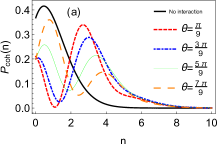
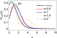
Figure 1: (Color online) Photon distribution $P_{coh}(n)$ of coherent state as a function of photon number $n$. $\vartheta=\frac{\pi}{3}$, $\varphi=\frac{\pi}{4}$, $r=1$. (a) $P_{coh}(n)$ plotted for $s=2,$ and for various weak value ($\langle\sigma_{x}\rangle_{w}=e^{\frac{i\pi}{3}}\tan\frac{\theta}{2}$) and no interaction case (black curve). (b) $P_{coh}(n)$ plotted for $\theta=\frac{7\pi}{9}$, and for various coupling strength $s$.

The conditional probability of finding $n$ photons after taking a postselected measurement for state $|\Psi\rangle$ is obtained from Eq. (12) by changing $|\Phi\rangle$ to a specific normalized state $|\Psi\rangle$. We plot the conditional probability of finding $n$ photons under the normalized state $|\Psi\rangle$ and the analytical results are shown in Fig. 1. As indicated in Fig. 1, the black solid line represents the photon distribution probability for the initial state of coherent pointer state before postselected measurement, and it has a Poisson probability distribution. However, as shown in Fig. 1 the postselected measurement can change the photons Poisson distribution with increasing the weak value and changing the interaction strength $s$. Furthermore, from Fig. 1(a) we can know that $P_{coh}(n)$ is larger, in postslected case for some small photon numbers regions rather than no interaction case.

For coherent state $|\alpha\rangle$ (Eq. (18)) the second-order correlation function $g^{(2)}(0)$ is equal to one, i.e.,$g^{(2)}(0)=1$ and the Mandel factor is equal to zero. Now we will calculate the $g_{coh}^{(2)}(0)$ and $Q_{m,coh}$ considering the final pointer state $|\Psi\rangle$ for coherent pointer state.The expectation value of photon number operator $\hat{n}=a^{\dagger}a$ under the state $|\Psi\rangle$ is

$$\langle n\rangle_{\Psi} =\frac{|\lambda|^{2}}{4}\{\text{$|1+\langle A\rangle_{w}|^{2}|\alpha+\frac{s}{2}|^{2}+|1-\langle A\rangle_{w}|^{2}|\alpha-\frac{s}{2}|^{2}$}$$

$$+2e^{-\frac{s^{2}}{2}}Re[e^{2isIm(\alpha)}(1-|\langle A\rangle_{w}|^{2}-2iIm\langle A\rangle_{w}))\times$$

$$(\alpha+\frac{s}{2})^{\ast}(\alpha-\frac{s}{2})]\}.$$ (21)

If we take $s=0$, then $\langle n\rangle_{s=0}=|\alpha|^{2}$ , this is the photon number for initial coherent state $|\alpha\rangle$. We also can get the expectation value of $\langle a^{\dagger 2}a^{2}\rangle$ as

$$\langle a^{\dagger 2}a^{2}\rangle_{\Psi} =\frac{|\lambda|^{2}}{4}\{|1+\langle A\rangle_{w}|^{2}|\alpha+\frac{s}{2}|^{4}+|1\!-\langle A\rangle_{w}|^{2}|\alpha-\frac{s}{2}|^{4}$$

$$+2e^{-\frac{s^{2}}{2}}Re[e^{2is|\alpha|\sin\phi}(1+\langle A\rangle_{w}^{\ast})(1-\langle A\rangle_{w})\times$$

$$(\alpha+\frac{s}{2})^{\ast 2}(\alpha-\frac{s}{2})^{2}]\}$$ (22)

If we take $s=0$ , it gives the value under the initial state $|\alpha\rangle$, i.g., $\langle a^{\dagger}a^{\dagger}aa\rangle_{s=0}=|\alpha|^{4}$. By substituting the above expressions to the Eqs. (13) and (14), we obtain the concrete expressions of $g_{coh}^{(2)}(0)$ and $Q_{m,coh}$, respectively. To investigating the effect of postselected measurement on the photon statistical properties of coherent state we plotted the analytical figures of $g_{coh}^{(2)}(0)$ and $Q_{m,coh}$, and the results are shown in Fig. 2.

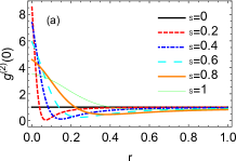
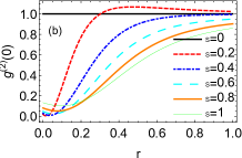
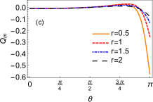
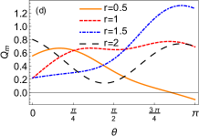
Figure 2: (Color online) Second-order correlation function $g_{coh}^{(2)}(0)$ and Mandel factor $Q_{m,coh}$ for coherent state after postselected measurement. Here, $\varphi=\frac{4\pi}{5}$, $\vartheta=\frac{\pi}{3}$. $g_{coh}^{(2)}(0)$ vs coherent state parameter $r$ for different interaction strength $s$ (black sold line represents for initial coherent state $|\alpha\rangle$ case) and for (a) $\theta=\frac{\pi}{3}$, or (b) $\theta=\frac{7\pi}{9}$ . Mandel factor $Q_{m,coh}$ plotted as a function of weak value for different $r$ of coherent state and for (c) $s=0.2$, or (d) $s=2$.

From Fig. 2 we can deduce that in postselected weak mesaurement region with large weak values (see Fig. 1(b) and (c)), the final state of the pointer state possessed sub-Poisson statistics $(0<g^{(2)}(0)<1$ and $-1<Q_{m}<0)$. From Fig. 1(d), we can see that in strong postselected measurement the system has super Poisson statistics $(g^{(2)}(0)>1$ and $Q_{m}>0)$. Thus, the results are summarized in Fig. 2 confirm that the postselected measurement can change the statistical properties of the coherent state significantly.

Since the coherent state is a minimum uncertainty state, there is no squeezing effect for coherent state $|\alpha\rangle$, i.e., $S_{\phi}=0$. Next, we will investigate the squeezing parameter $S_{\phi}^{coh}$ for $|\text{$\Psi$}\rangle$ of coherent pointer state. The expectation value of $X_{\phi,coh}$ under the state $|\Psi\rangle$ is given by

$$\langle X_{\phi,coh}\rangle_{\Psi} =\frac{|\lambda|^{2}}{\sqrt{2}}\{(1\!+|\langle A\rangle_{w}|^{2})|\alpha|\cos(\phi\!-\!\theta)\!+s\cos\phi Re[\langle A\rangle_{w}]$$

$$+\frac{1}{2}e^{-\frac{1}{2}s^{2}}\!\!Re[e^{2isIm(\alpha)}(1-\langle A\rangle_{w})(1+\langle A\rangle_{w}^{\ast})\times$$

$$(2r\cos(\vartheta-\phi)+is\sin\phi)].$$ (23)

If $s=0,$then the above expression reduced to the expectation value of $X_{\phi}$ under the initial coherent pointer state $|\alpha\rangle$, i.e., $\langle X_{\phi,coh}\rangle_{s=0}=Re[\alpha e^{-i\phi}]$. The expectation value of $X_{\phi,coh}^{2}$ with $|\Psi\rangle$ is given by

$$\langle X_{\phi,coh}^{2}\rangle_{\Psi} =\frac{1}{2}\langle(ae^{-i\phi}+a^{\dagger}e^{i\phi})(ae^{-i\phi}+a^{\dagger}e^{i\phi})\rangle$$

$$=\frac{1}{2}\left[\langle a^{2}\rangle e^{-2i\phi}+\langle a^{\dagger 2}\rangle e^{2i\phi}+2\langle a^{\dagger}a\rangle+1\right]$$

$$=\frac{1}{2}\left[2Re[\langle a^{2}\rangle e^{-2i\phi}]+2\langle n\rangle+1\right]$$ (24)

where

$$\langle a^{2}\rangle =\frac{|\lambda|^{2}}{4}\{|1+\langle A\rangle_{w}|^{2}(\alpha+\frac{s}{2})^{2}+|1-\langle A\rangle_{w}|^{2}(\alpha-\frac{s}{2})^{2}$$

$$+e^{2isIm(\alpha)}e^{-\frac{s^{2}}{2}}(1-\langle A\rangle_{w})(1+\langle A\rangle_{w}^{\ast})(\alpha-\frac{s}{2})^{2}$$

$$+e^{-2isIm(\alpha)}e^{-\frac{s^{2}}{2}}(1+\langle A\rangle_{w})(1-\langle A\rangle_{w}^{\ast})(\alpha+\frac{s}{2})^{2}\}.$$ (25)

The squeezing parameter $S_{\phi,coh}$ of state $|\Psi\rangle$ can be obtained by substituting the Eq. (23) and Eq. (24) into Eq. (17), and its analytical results listed in Fig. 3.

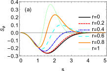
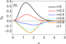
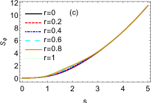
Figure 3: (Color online) The Squeezing parameter $S_{\phi,coh}$ for coherent state after postselected measurement. Here, $\varphi=\frac{4\pi}{5}$, $\vartheta=\frac{\pi}{3}$. $S_{\phi,coh}$vs interaction strength $s$ for various $r$ and $P$ quadrature of coherent state ($\phi=\frac{\pi}{2}$), but with different weak value: (a) $\theta=\frac{\pi}{9}$; (b) $\theta=\frac{7\pi}{9}$. (c) $S_{\phi,coh}$ plotted as function of interaction strength $s$ for various $r$ and for $\theta=\frac{\pi}{9}$, $\phi=0$ (represents the $X$ quadrature of coherent state). (d) $S_{\phi,coh}$ vs coherent state parameter $r$ for different weak values and for $\phi=\frac{\pi}{2}$, $s=2$.

We can observe from Fig. 3 that after postselected measurement the squeezing parameter of the initial coherent state changed dramatically, and can see the phase-dependent squeezing effect; the $X$ quadrature ($\phi=0$) of final state not squeezed (see Fig. 3(c)), but $P$ quadrature ($\phi=\frac{\pi}{2}$) of the final state have a squeezing effect for moderate interaction strengths (see Fig. 3(a),(b) and (d)) with any weak values.

III.2 Squeezed vacuum state

Our second pointer state is squeezed vacuum state. Squeezed states of the radiation field are generated by degenerate parametric down conversion in an optical cavity (Wu et al., 1986). The squeezed state have important applications in many quantum information processing tasks, including gravitational wave detection (Khalili et al., 2009; MckenzieSqueezed; Grote et al., 2016), quantum teleportation (Braunstein and Kimble, 1998; Milburn and Braunstein, 1999). Suppose that measuring device initially prepared in the squeezed vacuum state (Scully and Zubairy, 1997) which is defined by

$$|\xi\rangle=S(\xi)\left|0\right\rangle$$ (26)

where $S(\xi)=\exp(\frac{1}{2}\xi^{\ast}a^{2}-\frac{1}{2}\xi a^{\dagger 2})$, and $\xi=\eta e^{i\delta}$ is an arbitrary complex number with modulus $\eta$ and argument $\delta\in[0,2\pi]$. As indicated in Eq. (26), the squeezed vacuum state is generated by the action on the vacuum state $|0\rangle$ of the squeezing operator $S(\xi)$. After the postselected measurement processes as outlined in the Section.II , the normalized final pointer state can be written as

$$|\varphi\rangle=\frac{\kappa}{2}[(1+\langle A\rangle_{w})|\xi,\frac{s}{2}\rangle+(1-\langle A\rangle_{w})|\xi,-\frac{s}{2}\rangle],$$ (27)

where the normalization coefficient $\kappa$ is given by

$$\kappa=\sqrt{2}[1+|\langle A\rangle_{w}|^{2}+(1-|\langle A\rangle_{w}|^{2})e^{-\frac{1}{2}s^{2}|\cosh\eta+e^{i\delta}\sinh\eta|^{2}}]^{-\frac{1}{2}}$$ (28)

and we note that $|\xi,\pm\frac{s}{2}\rangle=D(\pm\frac{s}{2})S\left(\xi\right)|0\rangle$ is squeezed coherent state.

The probability amplitude of finding $n$ photons in a squeezed coherent state is given by

$$\langle n|\pm\frac{s}{2},\xi\rangle =\frac{1}{\sqrt{\cosh\eta}}\exp[-\frac{1}{2}|\pm\frac{s}{2}|^{2}-\frac{1}{2}(\pm\frac{s}{2})^{\ast 2}e^{i\delta}\tanh\eta]\times$$

$$\frac{\left(\frac{1}{2}e^{i\delta}\tanh\eta\right)^{\frac{n}{2}}}{\sqrt{n!}}H_{n}\left[\chi\left(e^{i\delta}\sinh(2r)\right)^{-\frac{1}{2}}\right]$$ (29)

with $\chi=\pm\frac{s}{2}\cosh\eta+(\pm\frac{s}{2})^{\ast}e^{i\delta}\sinh\eta$. To find the conditional probability of $n$ photons under the state $|\varphi\rangle$, we can use Eq. (12) by changing $|\Phi\rangle$ to $|\varphi\rangle$, and use Eq. (29). The effects of postselected measurement to the probability of finding $n$ photons for state $|\varphi\rangle$ is displayed in Fig. 4. The black thick curve in Fig. 4(a) corresponds to the conditional photon probability for initial pointer state $|\xi\rangle$. As illustrated in Fig. 4, the postselected measurement can change the photon distribution of the field, and in fewer photon number region the $P_{sq}(n)$ with the state $|\varphi\rangle$ is larger than no interaction case (see Fig. 4(a)). For definite squeeze parameter $\eta$ and weak measurement region ($s<1$) with large weak values, the $P_{qs}$is larger than strong measurement region ($s>1$), but its occurred probability is small.

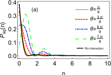
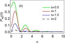
Figure 4: (Color online) Photon distribution $P_{sq}(n)$ of squeezed vacuum state after postselected measurement as a function of $n$. Here, $\delta=\frac{\pi}{3}$,$\varphi=\frac{\pi}{3}$, $\eta=0.5$. (a) $P_{sq}(n)$ is plotted for $s=1$, and for no interaction case (black curve) and various weak values. (b) $P_{sq}(n)$ is plotted for $\theta=\frac{7\pi}{9}$, and for various interaction strength $s$.

The second-order correlation function $g^{(2)}(0)$ and Mandel factor $Q_{m}$ of initial squeezed vacuum pointer state $|\xi\rangle$ is given by

$$g^{(2)}(0)=3+\frac{1}{\sinh^{2}\eta}$$ (30)

and

$$Q_{m}=1+2\sinh^{2}\eta,$$ (31)

respectively. It is clear that the number fluctuations of squeezed vacuum pointer state initially are super-Poissonian, and for all value of $\eta$ both $g^{(2)}(0)$ and $Q_{m}$ can’t take the values to possess the sub-Poissonian statistics which is a nonclassical property of the field. Now, we will study the effect of postselected measurement to $g^{(2)}(0)$ and $Q_{m}$ of squeezed vacuum pointer state under the normalized final pointer state $|\varphi\rangle$. The expectation value of photon number operator $a^{\dagger}a$ and the $(a^{\dagger}a)^{2}$ under the final state $|\varphi\rangle$ can be calculated, and their explicit expressions are given in Appendix. A (Since the expressions are too cumbersome to write here, we displayed them in the Appendix ).

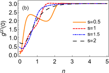
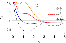
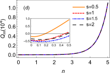
Figure 5: (Color online) Second-order correlation function $g_{sq}^{(2)}(0)$ and Mandel factor $Q_{m,sq}$ of squeezed vacuum state after postselected measurement. Here, $\varphi=\frac{\pi}{3}$,$\delta=\frac{\pi}{3}$. (a) $g_{sq}^{(2)}(0)$ vs in interaction strength $s$ for different weak values and for $\eta=0.2$. (b) $g_{sq}^{(2)}(0)$ plotted as function of squeezed vacuum state parameter $\eta$ for various interaction strength and for $\theta=\frac{7\pi}{9}$. (c) $Q_{m,sq}$ vs in interaction strength $s$ for different weak values and for $\eta=0.2$. (d) $Q_{m,sq}$ plotted as function of squeezed vacuum state parameter $\eta$ for various interaction strength and for $\theta=\frac{7\pi}{9}$, and the inset in this figure depicts the curves in the interval $\eta\in[0,0.5]$.

The analytical results for $g_{sq}^{(2)}(0)$ and $Q_{m,sq}$ under the state $|\varphi\rangle$ are presented in Fig. 5. It can be observed from Fig. 5(a) and (c) that both $g_{sq}^{(2)}(0)$ and $Q_{m,sq}$ can take the values, which only sub-Poisson radiation field can possess where the region $s\apprge 0.5$ and for large weak values. For definite measurement strength $s$ and larger weak value, the value $g_{sq}^{(2)}(0)$ is lower than one and the value of $Q_{m,sq}$ is less than zero when the squeezed state parameter $\eta$ is less than one (see Fig. 5(b) and (d)). Thus, it is apparent that the postselected measurement dramatically changed the photon statistical properties of initial squeezed pointer state $|\xi\rangle$.

The squeezing parameter $S_{\phi}$ of initial squeezed vacuum state $|\xi\rangle$ can be calculated by using Eqs. (15-17) and Eq. (33), and written as

$$S_{\phi} =\frac{1}{2}\left[\cosh^{2}\eta-\sinh(2\eta)\cos(2\phi-\delta)+\sinh^{2}\eta\right]-\frac{1}{2}.$$ (32)

It is evident from Eq. (32) that the squeezing effect of squeezed vacuum state is phase-dependent: (i) if $\phi=\frac{\delta}{2}$, then $S_{\phi}=-\frac{1}{2}(1-e^{-2\eta})$, it has squeezing effect for $\eta>0$; (ii) if $\phi=\frac{\delta}{2}+\frac{\pi}{2}$ , then $S_{\phi}=\frac{1}{2}(e^{2\eta}-1)$, there is no squeezing effect. This reveals that it spread out the quadrature $X_{\phi=\frac{\delta}{2}}$ and at the same time squeezes the quadrature $X_{\phi=\frac{\delta}{2}+\frac{\pi}{2}}$.

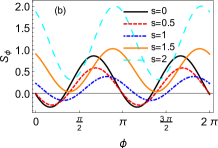
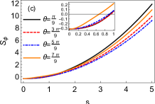
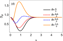
Figure 6: (Color online) Squeezing parameter $S_{\phi,sq}$ of squeezed vacuum state after postselected measurement. Here, $\varphi=\frac{\pi}{3}$. (a) $S_{\phi}$ vs $\eta$ of squeezed vacuum state for different interaction strength $s$ and for $\delta=\phi=0$, $\theta=\frac{\pi}{9}$. (b)$S_{\phi,sq}$ plotted as a function of $\phi$ for various interaction strength $s$ and for $\eta=0.5,\delta=\frac{\pi}{3}$, and $\theta=\frac{\pi}{9}$. $S_{\phi,sq}$ vs interaction strength $s$ for different weak values and for $\delta=0$ and $\eta=0.5$, but with different $\phi$: (c) $\phi=0$; (d) $\phi=\frac{\pi}{2}$. The inset in (c) depicts the curves in the interval $s\in(0,1]$.

Squeezing parameter $S_{\phi,sq}$ of final normalized state $|\varphi\rangle$ after postselected von-Nuemann measurement can be calculated as the same processes of initial state $|\xi\rangle$, and the analytical results showed in Fig. 6. According to Fig. 6 (a) and (b), the postselected measurement would have a negative effect on the squeezing effect of squeezed vacuum state since $S_{\phi,sq}$ gradually becoming larger with increasing the measurement strength $s$. However, as indicated in Fig. 6(c), in weak measurement regime where $0<s<1$ postselected measurement still has the effects on the squeezing of squeezed vacuum pointer state. As mentioned earlier the squeezing effect of squeezed vacuum state is phase-dependent, and the postselected measurement has no positive effect on the squeezing of $X_{\phi=\frac{\pi}{2}}$ quadrature (see Fig. 6(d)).

III.3 Schrödinger cat state

In the previous two subsections, we already confirmed that postselected measurement characterized by a weak value can really change the statistical and squeezing effect of single-mode radiation fields. To further increase the reliability of our conclusions, in this subsection, we check the same phenomena by taking the Schrödinger cat state as a pointer. Schrödinger’s cat is a gedanken experiment in quantum physics was proposed by Schrödinger in 1935 (Schr?dinger, 1935), and its corresponding state is called Schrödinger cat state. Schrödinger cat state play significant role not only in fundamental tests of quantum theory (Sanders, 1992; Wenger et al., 2003; Jeong et al., 2003; Stobińska et al., 2007), but also in many quantum information processing such as quantum computation (Ralph et al., 2003), quantum teleportation (van Enk and Hirota, 2001; Jeong et al., 2001) and precision measurements (Munro et al., 2002). The Schrödinger cat state is composed by the superposition of two coherent correlated states moving in the opposite directions, and defined as (Agarwal, 2013)

$$|\varTheta\rangle=K\left(|\alpha\rangle+e^{i\omega}|-\alpha\rangle\right)$$ (33)

where

$$K=\left[2+2e^{-2|\alpha|^{2}}\cos\omega\right]^{-\frac{1}{2}}$$ (34)

is normalization constant and $\alpha=re^{i\delta}$ is a coherent state parameter with modulus $r$ and argument $\delta$. The normalized final state of Schrödinger cat state after the postselected weak measurement is given by taking $|\phi\rangle=|\varTheta\rangle$ in Eq. (6), i.e.,

$$|\chi\rangle =\frac{\kappa}{2}\left[\left(1+\langle A\rangle_{w}\right)D\left(\frac{s}{2}\right)+\left(1-\langle A\rangle_{w}\right)D\left(-\frac{s}{2}\right)\right]\left|\Theta\right\rangle$$ (35)

with normalization coefficient

$$\kappa^{-2} =\frac{1}{2}(1+|\langle A\rangle_{w}|^{2})+K^{2}(1-|\langle A\rangle_{w}|^{2})\cos(2sIm[\alpha])e^{-\frac{s^{2}}{2}}$$

$$+\frac{K^{2}}{2}\Re[(1-\langle A\rangle_{w})(1+\langle A\rangle_{w}^{\ast})\times$$

$$(e^{i\omega}e^{-\frac{1}{2}|2\alpha+s|^{2}}+e^{-i\omega}e^{-\frac{1}{2}|2\alpha-s|^{2}})].$$ (36)

Here, we have to mention that $\omega\in[0,2\pi]$, and when $\omega=0$ ($\omega=\pi$) it is called even (odd) Schrödinger cat state. Similarly to the previous two cases, the conditional probability $P_{sh}(n)$ of Schrödinger cat state can be obtained by replacing the $|\phi\rangle$ in Eq. (6) to $|\chi\rangle$, and the analytical results of even Schrödinger cat state is presented in Fig. 7. As shown in Fig. 7, the postselected measurement can change photon distribution of the field, and in fewer photon regions with large weak values, $P_{sh}(n)$ larger than initial photon distribution of Schrodinger even cat state. By comparing Fig. 7 and Fig. 4 we also can get the same common sense that the even Schrödinger cat state have similar properties as a squeezed state.

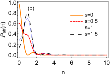
Figure 7: (Color online) Photon distribution $P_{sh}(n)$ of squeezed state as a function of photon number $n$. Here, $\delta=\frac{\pi}{3}$,$\varphi=\frac{\pi}{3}$,$\omega=0$, $r=0.5$ (a) $P_{sh}(n)$ is plotted for $s=1$, and for various weak values. (b) $P_{sh}(n)$ is plotted for $\theta=\frac{7\pi}{9}$, and for various interaction strength $s$.

The Mandel factor and second-order correlation function for Schrodinger cat state are given by

$$Q_{m} =\frac{4|\alpha|^{2}e^{-2|\alpha|^{2}}\cos\omega}{1-e^{-4|\alpha|^{2}}\cos^{2}\omega}$$ (37)

and

$$g^{(2)}(0) =1+\frac{4e^{-2|\alpha|^{2}}\cos\omega}{(1-e^{-2|\alpha|^{2}}\cos\omega)^{2}},$$ (38)

respectively. It is apparent that both $g^{(2)}(0)$ and $Q_{m}$ have sub-Poisson statistics when $\cos\omega<0$ ($\frac{\pi}{2}<\omega<\frac{3\pi}{2}$).

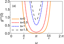
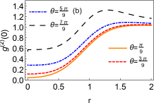
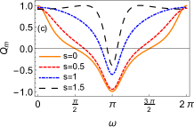
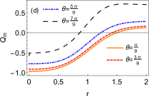
Figure 8: (Color online) second-ordercorrelation function $g_{sh}^{(2)}(0)$ and Mandel factor $Q_{m,sh}$ of Schrödinger state after postselected measurement. Here $\varphi=0$, $\delta=0$. (a) $g_{sh}^{(2)}(0)$ plotted as function $\omega$ of Schrödinger cat state for various interaction strength $s$ and for $\theta=\frac{\pi}{9}$, $r=0.3$. (b) $g_{sh}^{(2)}(0)$ vs parameter $r$ of Schrödinger cat state for different weak values and for and $s=0.5$, $\omega=\pi$. (c) $Q_{m,sh}$ plotted as function $\omega$ of Schrödinger cat state for various interaction strength $s$ and for $\theta=\frac{\pi}{9}$, $r=0.3$. (d) $Q_{m,sh}$ vs parameter $r$ of Schrödinger cat state for different weak values and for $s=0.5$, $\omega=\pi$.

The $g_{sh}^{(2)}(0)$ and $Q_{m,sh}$ of Schrödinger cat state can be calculated by using Eq. (13) and Eq. (14) with normalized final pointer state $|\chi\rangle$. As indicated in Fig. 8, after postselected measurement, the statistical property of Schrödinger cat state changed from sub-Poisson to super-Poisson gradually with increasing the interaction strength and weak value. However, as we can see in Fig. 8(b) and (d), in postselected weak measurement regime, where $0<s<1$, would give the best performance for nonclassicality of odd Schrödinger cat state with small coherent state modulus $r$.

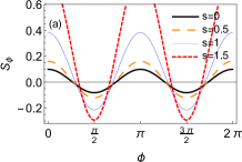
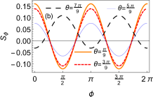
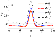
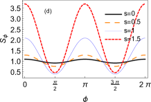
Figure 9: (Color online) Squeezing parameter $S_{\phi,sh}$ of Schrödinger cat state. Here $\varphi=0$, $\delta=0$, $r=0.3$. $S_{\phi,sh}$ of even Schrödinger cat state ($\omega=0$) vs squeezing parameter angle $\phi$ for different interaction strength and for $\theta=\frac{\pi}{9}$ in (a); for different weak values and for $s=0.5$ in (b), respectively. (c) $S_{\phi,sh}$ plotted as a function of $\omega$ for various weak values and for $s=0.5$, $\phi=\frac{\pi}{2}$. (d) $S_{\phi,sh}$of odd Schrödinger cat state ($\omega=\pi$) vs squeezing parameter angle $\phi$ for different interaction strength and for $\theta=\frac{\pi}{9}.$

The squeezing parameter of initial Schrödinger cat state $|\varTheta\rangle$ reads as (Agarwal, 2013)

$$S_{\phi}^{in} =\frac{|\alpha|^{2}e^{-4|\alpha|^{2}}}{(1+e^{-2|\alpha|^{2}}\cos\omega)^{2}}\times$$

$$\left[1+\left(\cos 2\phi(e^{2|\alpha|^{2}}+\cos\omega)^{2}+\sin^{2}\omega\cos^{2}\phi-1\right)\right]$$ (39)

From this expression, we can deduce that the squeezing effect of initial Schrödinger cat state is also phase-dependent similar to the squeezed vacuum state, and the quadrature of the field will be squeezed only when the inequality $\cos 2\phi<\frac{\sin^{2}\omega\cos^{2}\phi-1}{(\cos\omega+e^{2|\alpha|^{2}})^{2}}$ satisfied. The details of this squeezing effect presented in Fig. 9 (a)(see the black solid curve).

The analytic expression of $S_{\phi,sch}$ for Schrödinger cat state after postselected measurement can be achieved using final normalized state $|\chi\rangle$, and the analytical results are summarized in Fig. (9). As indicated in Fig. 9, after postselected measurement, the squeezing effect of Schrödinger cat state still depends on phase $\phi$, and the squeezing effect of both even and odd Schrödinger cat states are increased with increasing the interaction strength $s$ and for small weak values (see Fig. 9 (a), (b) and (d)). However, the odd Schrödinger cat pointer state has no squeezing effect (see Fig. 9 (c) and (d)).

IV Conclusion and remarks

In summary, we investigated the effects of postselected measurement characterized by postselection and weak value on the statistical properties and squeezing effects of single-mode radiation fields. To achieve our goal, we take the coherent state, squeezed vacuum state and Schrödinger cat state as a pointer, and their polarization degrees of freedom as measures system, respectively. We derived analytical expressions of those pointer state’s normalized final state after postselected measurement considering all interaction strengths between pointer and measured system. We separately presented the exact expressions of photon distributions, second-order correlation functions, Mandel factors and squeezing parameters of the above three typical single-mode radiation fields for corresponding final pointer states, and plotted the figures to analyze the results.

We found that the photon distributions of those three pointer states changed significantly after postelected measurement, especially the coherent pointer state. We showed that postselected measurement changed the photon statistics and squeezing effect of coherent state dramatically, and noticed that the amplification effect of weak value played a major role in this process. We also showed that the postselected measurement changed the photon statistics of squeezed vacuum state from super-Poisson to sub-Poisson for large weak values, and moderate interaction strengths. Whereas, the photon statistics of Schrödinger cat state changed from sub-Poisson to super-Poisson with increasing the interaction strength. In accordance with previous findings, the squeezing effects of squeezed vacuum and Schrodinger cat pointer states are still, phase-dependent and the squeezing effect of squeezed vacuum pointer is decreased with increasing the interaction strength. On the contrary, the squeezing effect of even Schrödinger cat state is increased with increasing the interaction strength for small weak values compared with the initial pointer state case.

This work belong to the state optimization by using postselected von-neumann measurement. Those properties of radiation fields we investigated in this paper, are directly effect on the implementations of the important quantum information processing which mentioned in introduction part. Thus, we anticipate that the results showed in this research can be useful to provide other effective methods for studying the related quantum information processing.

In our current research, we only consider the three typical single-mode radiation fields to investigate the effects of postselected von-Neuman measurement on their inherent properties, but real light beams are in fact the time-dependent and the representation of time dependence requires the use of two or more modes of the optical systems. Thus, it would be interesting to check the effects of postselected von-neumann measurement on other useful radiation fields in quantum optics and quantum information processing such as single photon-added (Zavatta et al., 2004; Barbieri et al., 2010) and -subtracted (Biswas and Agarwal, 2007) states, pair-coherent state (two-mode field) (Agarwal, 1988; Xin et al., 1994, 1996; Yuen, 1976) and other multimode radiation fields (Blow et al., 1990), respectively.

Appendix A The explicit expressions of some quantities

1. For squeezed vacuum pointer state: The expectation value of photon number operator $a^{\dagger}a$ under the state $|\chi\rangle$ is given by

$$\langle a^{\dagger}a\rangle_{\varphi}=\frac{\text{$|\kappa|^{2}$}}{4}\{2(1+|\langle A\rangle_{w}|^{2})(\frac{s^{2}}{4}+\sinh^{2}\eta)+2Re[(1-\text{$\langle A\rangle_{w}$})(1+\langle A\rangle_{w})^{\ast}I]\}$$ (40)

with

$$I=\exp[-\frac{s^{2}}{2}|\cosh\eta+e^{i\delta}\sinh\eta|^{2}](\sinh^{2}\eta+\frac{s^{2}}{4}-\frac{s^{2}}{2}(1+i\sin\delta\sinh 2\eta))$$

In calculating the squeezing parameter, we use $\langle X_{\phi}\rangle_{\varphi}$ and $\langle X_{\phi}^{2}\rangle_{\varphi}$, and their expressions are given by

$$\langle X_{\phi}\rangle_{\varphi} =s\frac{|\kappa|^{2}}{4\sqrt{2}}\{\cos\phi|1+\langle A\rangle_{w}|^{2}-\cos\phi|1+\langle A\rangle_{w}|^{2}$$

$$+2\exp[-\frac{s^{2}}{2}|\cosh\eta+e^{i\delta}\sinh\eta|^{2}]Re[e^{-i\theta}(1+\langle A\rangle_{w})(1-\langle A\rangle_{w})^{\ast}(\cosh^{2}\eta+\frac{1}{2}e^{i\delta}\sinh 2\eta-\frac{1}{2})]$$

$$-2\exp[-\frac{s^{2}}{2}|\cosh\eta+e^{i\delta}\sinh\eta|^{2}]Re\{e^{i\theta}(1+\langle A\rangle_{w})^{\ast}(1-\langle A\rangle_{w})[\cosh^{2}\eta+e^{i\delta}\frac{1}{2}\sinh 2\eta-\frac{1}{2}]\}$$

and

$$\langle X_{\theta}^{2}\rangle =\frac{1}{2}[2Re(IIe^{-2i\phi})+2\langle a^{\dagger}a\rangle+1]$$ (41)

with

$$II =\frac{|\kappa|^{2}}{4}\{\left(\frac{s^{2}}{4}-\frac{1}{2}\sinh(2\eta)e^{-i\delta}\right)|1+\langle A\rangle_{w}|^{2}+\left(\frac{s^{2}}{4}-\frac{1}{2}\sinh(2\eta)e^{-i\delta}\right)|1-\langle A\rangle_{w}|^{2}$$

$$+(1-|\langle A\rangle_{w}|^{2})III\}$$

where

$$I II=\frac{s^{2}}{4}+s^{2}(\frac{1}{2}e^{-i\delta}\sinh 2\eta+\sinh^{2}\eta)+s^{2}(\cosh\eta+e^{i\delta}\sinh\eta)^{2}e^{-2i\delta}\sinh^{2}\eta$$

$$-e^{-i\delta}\frac{1}{2}\sinh 2\eta\}\exp[-\frac{s^{2}}{2}|\cosh\eta+e^{i\delta}\sinh\eta|^{2}]$$

respectively.

2. For Schrödinger cat pointer state: The expectation value of photon number operator $a^{\dagger}a$ and $a^{\dagger 2}a^{2}$ under the state $|\chi\rangle$ is given by

$$\langle a^{\dagger}a\rangle_{\chi} =\frac{|\kappa|^{2}K^{2}}{4}\{|1+\langle A\rangle_{w}|^{2}\left[|\alpha+\frac{s}{2}|^{2}+|-\alpha+\frac{s}{2}|^{2}+e^{i\omega}(\alpha+\frac{s}{2})^{\ast}(-\alpha+\frac{s}{2})e^{-2|\alpha|^{2}}+e^{-i\omega}(-\alpha+\frac{s}{2})^{\ast}(\alpha+\frac{s}{2})e^{-2|\alpha|^{2}}\right]$$

$$+|1-\langle A\rangle_{w}|^{2}\left[|\alpha-\frac{s}{2}|^{2}+|\alpha+\frac{s}{2}|^{2}-e^{i\omega}(\alpha-\frac{s}{2})^{\ast}(\alpha+\frac{s}{2})e^{-2|\alpha|^{2}}-e^{-i\omega}(\alpha+\frac{s}{2})^{\ast}(\alpha-\frac{s}{2})e^{-2|\alpha|^{2}}\right]$$

$$-2Re[(e^{i\omega}|\alpha+\frac{s}{2}|^{2}e^{-2|\alpha+\frac{s}{2}|^{2}}+e^{-i\omega}e^{-2|\alpha-\frac{s}{2}|^{2}}|\alpha-\frac{s}{2}|^{2}-2e^{-\frac{s^{2}}{2}}Re[e^{2isIm(\alpha)}(\alpha+\frac{s}{2})^{\ast}(\alpha-\frac{s}{2})])\times$$

$$(1-\langle A\rangle_{w})(1+\langle A\rangle_{w})^{\ast}]\},$$ (42)

and

$$\langle a^{\dagger 2}a^{2}\rangle_{\chi} =\frac{|\kappa|^{2}K^{2}}{4}\{|1+\langle A\rangle_{w}|^{2}\left[|\alpha+\frac{s}{2}|^{4}+|-\alpha+\frac{s}{2}|^{4}+e^{i\omega}(\alpha^{\ast}+\frac{s}{2})^{2}(-\alpha+\frac{s}{2})^{2}e^{-2|\alpha|^{2}}+e^{-i\omega}(-\alpha^{\ast}+\frac{s}{2})^{2}(\alpha+\frac{s}{2})^{2}e^{-2|\alpha|^{2}}\right]$$

$$+|1-\langle A\rangle_{w}|^{2}\left[|\alpha-\frac{s}{2}|^{4}+|\alpha+\frac{s}{2}|^{4}+e^{i\omega}e^{-2|\alpha|^{2}}(\alpha^{\ast}-\frac{s}{2})^{2}(\alpha+\frac{s}{2})^{2}+e^{-i\omega}e^{-2|\alpha|^{2}}(\alpha^{\ast}+\frac{s}{2})(\alpha-\frac{s}{2})^{2}\right]$$

$$+2Re[(e^{i\omega}|\alpha+\frac{s}{2}|^{4}e^{-2|\alpha+\frac{s}{2}|^{2}}+e^{-i\omega}|\alpha-\frac{s}{2}|^{4}e^{-2|\alpha-\frac{s}{2}|^{2}}+2e^{-\frac{s^{2}}{2}}Re[e^{2isIm(\alpha)}(\alpha^{\ast}+\frac{s}{2})^{2}(\alpha-\frac{s}{2})^{2}])\times$$

$$(1-\langle A\rangle_{w})(1+\langle A\rangle_{w})^{\ast}]\},$$ (43)

respectively. In calculating the squeezing parameter, we use $\langle X_{\phi}\rangle_{\chi}$ and $\langle X_{\phi}^{2}\rangle_{\chi}$, and their expressions are given by

$$\langle X_{\phi}\rangle_{\chi} =\sqrt{2}Re[\langle a\rangle_{\chi}e^{-i\phi}]$$

with

$$\langle a\rangle_{\chi} =\frac{|\kappa|^{2}K^{2}}{4}\{|1+\langle A\rangle_{w}|^{2}[s+e^{i\phi}(-\alpha+\frac{s}{2})e^{-2|\alpha|^{2}}+e^{-i\phi}(\alpha+\frac{s}{2})e^{-2|\alpha|^{2}}]$$

$$+|1-\langle A\rangle_{w}|^{2}[-s-e^{i\phi}(\alpha+\frac{s}{2})e^{-2|\alpha|^{2}}+e^{-i\phi}(\alpha-\frac{s}{2})e^{-2|\alpha|^{2}}]$$

$$+(1-\langle A\rangle_{w})(1+\langle A\rangle_{w})^{\ast}[(2i\alpha\sin(2sIm[\alpha])-s\cos(2sIm[\alpha]))e^{-\frac{1}{2}s^{2}}-e^{i\phi}(\alpha+\frac{s}{2})e^{-\frac{1}{2}|2\alpha+s|^{2}}+e^{-i\phi}(\alpha-\frac{s}{2})e^{-\frac{1}{2}|2\alpha-s|^{2}}]$$

$$+(1-\langle A\rangle_{w})^{\ast}(1+\langle A\rangle_{w})[(-2i\alpha\sin(2sIm[\alpha])+s\cos(2sIm[\alpha]))e^{-\frac{1}{2}s^{2}}+e^{i\phi}(-\alpha+\frac{s}{2})e^{-\frac{1}{2}|2\alpha-s|^{2}}+e^{-i\phi}(\alpha+\frac{s}{2})e^{-\frac{1}{2}|2\alpha+s|^{2}}]\}$$

and

$$\langle X_{\phi}^{2}\rangle_{\chi} =\frac{1}{2}[2\langle a^{\dagger}a\rangle_{\chi}+2Re[\langle a^{2}\rangle_{\chi}e^{-2i\phi}]+1]$$

with

$$\langle a^{2}\rangle_{\chi} =\frac{|\kappa|^{2}K^{2}}{4}\{|1+\langle A\rangle_{w}|^{2}\left[2(\alpha^{2}+\frac{s^{2}}{4})+e^{i\omega}e^{-2|\alpha|^{2}}(-\alpha+\frac{s}{2})^{2}+e^{-i\omega}e^{-2|\alpha|^{2}}(\alpha+\frac{s}{2})^{2}\right]$$

$$+|1-\langle A\rangle_{w}|^{2}\left[2(\alpha^{2}+\frac{s^{2}}{4})+e^{i\omega}e^{-2|\alpha|^{2}}(\alpha+\frac{s}{2})^{2}+e^{-i\omega}e^{-2|\alpha|^{2}}(\alpha-\frac{s}{2})^{2}\right]$$

$$\!\!+(1-\!\langle A\rangle_{w})(1\!+\!\langle A\rangle_{w})^{\ast}[2e^{-\frac{s^{2}}{4}}(\cos(2sIm[\alpha])(\alpha^{2}+\frac{s^{2}}{4})-\!is\alpha\sin(2sIm[\alpha]))\!+\!e^{-i\omega}(\alpha-\frac{s}{2})^{2}e^{-2|\alpha-\frac{s}{2}|^{2}}\!+e^{i\omega}(\alpha+\frac{s}{2})^{2}e^{-2|\alpha+\frac{s}{2}|^{2}}]$$

$$\!\!+\!(1+\!\langle A\rangle_{w})(1-\!\langle A\rangle_{w})^{\ast}[2e^{-\frac{s^{2}}{4}}(\cos(2sIm[\alpha])(\alpha^{2}+\frac{s^{2}}{4})\!-\!is\alpha\sin(2sIm[\alpha]))\!+\!e^{i\omega}(\alpha-\frac{s}{2})^{2}e^{-2|\alpha-\frac{s}{2}|^{2}}\!+e^{-i\omega}(\alpha+\frac{s}{2})^{2}e^{-2|\alpha+\frac{s}{2}|^{2}}]\},$$ (44)

respectively.

References

- Aharonov et al. (1988) Y. Aharonov, D. Z. Albert, and L. Vaidman, Phys. Rev. Lett. 60, 1351 (1988).
- von Neumann J (1955) von Neumann J, Mathematical Foundations of Quantum Mechanics (Princeton University Press, Princeton, NJ, 1955).
- Ritchie et al. (1991) N. Ritchie, J. Story, and R. Hulet, Phys. Rev. Lett. 66, 1107 (1991).
- Kofman et al. (2012) A. G. Kofman, S. Ashhab, and F. Nori, Phys. Rep. 520, 43 (2012).
- Dressel et al. (2014) J. Dressel, M. Malik, F. M. Miatto, A. N. Jordan, and R. W. Boyd, Rev. Mod. Phys. 86, 307 (2014).
- Aharonov and Botero (2005) Y. Aharonov and A. Botero, Phys. Rev. A 72, 052111 (2005).
- Di Lorenzo and Egues (2008) A. Di Lorenzo and J. C. Egues, Phys. Rev. A 77, 042108 (2008).
- Pan and Matzkin (2012) A. K. Pan and A. Matzkin, Phys. Rev. A 85, 022122 (2012).
- Nakamura et al. (2012) K. Nakamura, A. Nishizawa, and M.-K. Fujimoto, Phys. Rev. A 85, 012113 (2012).
- Turek et al. (2015a) Y. Turek, H. Kobayashi, T. Akutsu, C.-P. Sun, and Y. Shikano, New J. Phys. 17, 083029 (2015a).
- de Lima Bernardo et al. (2014a) B. de Lima Bernardo, S. Azevedo, and A. Rosas, Opt. Commun. 331, 194 (2014a).
- Turek et al. (2015b) Y. Turek, W. Maimaiti, Y. Shikano, C.-P. Sun, and M. Al-Amri, Phys. Rev. A 92, 022109 (2015b).
- Pang and Brun (2015) S. Pang and T. A. Brun, Phys. Rev. Lett. 115, 120401 (2015).
- Turek and Yusufu (2018) Y. Turek and T. Yusufu, Eur. Phys. J. D 72, 202 (2018).
- Kedem and Vaidman (2010) Y. Kedem and L. Vaidman, Phys. Rev. Lett. 105, 230401 (2010).
- Buller and Collins (2010) G. S. Buller and R. J. Collins, Meas. Sci. Technol 21, 12002 (2010).
- Khalili et al. (2009) F. Y. Khalili, H. Miao, and Y. Chen, Phys. Rev. D 80, 042006 (2009).
- Grote et al. (2016) H. Grote, M. Weinert, R. X. Adhikari, C. Affeldt, and H. Wittel, Opt. Express 24, 20107 (2016).
- Braunstein and Kimble (1998) S. L. Braunstein and H. J. Kimble, Phys. Rev. Lett. 80, 869 (1998).
- Milburn and Braunstein (1999) G. J. Milburn and S. L. Braunstein, Phys. Rev. A 60, 937 (1999).
- Jeong et al. (2001) H. Jeong, M. S. Kim, and J. Lee, Phys. Rev. A 64, 052308 (2001).
- van Enk and Hirota (2001) S. J. van Enk and O. Hirota, Phys. Rev. A 64, 022313 (2001).
- Ralph et al. (2003) T. C. Ralph, A. Gilchrist, G. J. Milburn, W. J. Munro, and S. Glancy, Phys. Rev. A 68, 042319 (2003).
- Muschik et al. (2006) C. A. Muschik, K. Hammerer, E. S. Polzik, and J. I. Cirac, Phys. Rev. A 73, 062329 (2006).
- Li et al. (2013) L. Li, Y. O. Dudin, and A. Kuzmich, Nature 498, 466 (2013).
- Hacker et al. (2019) B. Hacker, S. Welte, S. Daiss, A. Shaukat, S. Ritter, L. Li, and G. Rempe, Nat. Photon. 13, 110 (2019).
- Munro et al. (2002) W. J. Munro, K. Nemoto, G. J. Milburn, and S. L. Braunstein, Phys. Rev. A 66, 023819 (2002).
- Glauber (1963) R. J. Glauber, Phys. Rev. 131, 2766 (1963).
- Carranza and Gerry (2012) R. Carranza and C. C. Gerry, J. Opt. Soc. Am. B 29, 2581 (2012).
- Andersen et al. (2016) U. L. Andersen, T. Gehring, C. Marquardt, and G. Leuchs, Phys. Scripta. 91, 053001 (2016).
- Monroe et al. (1996) C. Monroe, D. M. Meekhof, B. E. King, and D. J. Wineland, Science 272, 1131 (1996).
- Ourjoumtsev et al. (2007) A. Ourjoumtsev, H. Jeong, R. Tualle-Brouri, and P. Grangier, Nature 448, 784 (2007).
- Haroche (2013) S. Haroche, Rev. Mod. Phys. 85, 1083 (2013).
- Starling et al. (2009) D. J. Starling, P. B. Dixon, A. N. Jordan, and J. C. Howell, Phys. Rev. A 80, 041803 (2009).
- Hosten and Kwiat (2008) O. Hosten and P. Kwiat, Science 319, 787 (2008).
- Dixon et al. (2009) P. B. Dixon, D. J. Starling, A. N. Jordan, and J. C. Howell, Phys. Rev. Lett. 102, 173601 (2009).
- Zhou et al. (2013) L. Zhou, Y. Turek, C. P. Sun, and F. Nori, Phys. Rev. A 88, 053815 (2013).
- Starling et al. (2010) D. J. Starling, P. B. Dixon, A. N. Jordan, and J. C. Howell, Phys. Rev. A 82, 063822 (2010).
- Magaña Loaiza et al. (2014) O. S. Magaña Loaiza, M. Mirhosseini, B. Rodenburg, and R. W. Boyd, Phys. Rev. Lett. 112, 200401 (2014).
- Pfeifer and Fischer (2011) M. Pfeifer and P. Fischer, Opt. Express 19, 16508 (2011).
- de Lima Bernardo et al. (2014b) B. de Lima Bernardo, S. Azevedo, and A. Rosas, Phys. Lett. A 378, 2029 (2014b).
- Viza et al. (2013) G. I. Viza, J. Martínez-Rincón, G. A. Howland, H. Frostig, I. Shomroni, B. Dayan, and J. C. Howell, Opt. Lett. 38, 2949 (2013).
- Egan and Stone (2012) P. Egan and J. A. Stone, Opt. Lett. 37, 4991 (2012).
- Aharonov and Rohrlich (2005) Y. Aharonov and D. Rohrlich, Quantum Paradoxes-Quantum Theory for the Perplexed (Wiley-VCH, Weinheim, 2005).
- Gerry and Knight (2005) C. Gerry and P. Knight, Introductory Quantum Optics (Cambridge University Press, Cambridge, England, 2005).
- Mandel (1979) L. Mandel, Opt. Lett. 4, 205 (1979).
- Agarwal (2013) G. Agarwal, Quantum Optics (Cambridge University Press, Cambridge, England, 2013).
- Schr?dinger (1926) E. Schr?dinger, Naturwissenschaften 14, 664 (1926).
- Klauder and Skagerstam (1985) J. Klauder and B. Skagerstam, Coherent States (World scientific, 1985).
- Perelomov (1986) Perelomov, Generalized Coherent States and Their Applications (Springer, Berlin, Heidelberg, 1986).
- Scully and Zubairy (1997) M. Scully and M. Zubairy, Quantum Optics (Cambridge University Press, Cambridge, England, 1997).
- Wu et al. (1986) L.-A. Wu, H. J. Kimble, J. L. Hall, and H. Wu, Phys. Rev. Lett. 57, 2520 (1986).
- Schr?dinger (1935) E. Schr?dinger, Naturwissenschaften 23, 807 (1935).
- Sanders (1992) B. C. Sanders, Phys. Rev. A 45, 6811 (1992).
- Wenger et al. (2003) J. Wenger, M. Hafezi, F. Grosshans, R. Tualle-Brouri, and P. Grangier, Phys. Rev. A 67, 012105 (2003).
- Jeong et al. (2003) H. Jeong, W. Son, M. S. Kim, D. Ahn, and C. Brukner, Phys. Rev. A 67, 012106 (2003).
- Stobińska et al. (2007) M. Stobińska, H. Jeong, and T. C. Ralph, Phys. Rev. A 75, 052105 (2007).
- Zavatta et al. (2004) A. Zavatta, S. Viciani, and M. Bellini, Science 306, 660 (2004).
- Barbieri et al. (2010) M. Barbieri, N. Spagnolo, M. G. Genoni, F. Ferreyrol, R. Blandino, M. G. A. Paris, P. Grangier, and R. Tualle-Brouri, Phys. Rev. A 82, 063833 (2010).
- Biswas and Agarwal (2007) A. Biswas and G. S. Agarwal, Phys. Rev. A 75, 032104 (2007).
- Agarwal (1988) G. S. Agarwal, Journal of The Optical Society of America B-optical Physics 5, 1940 (1988).
- Xin et al. (1994) Z. Z. Xin, D. B. Wang, M. Hirayama, and K. Matumoto, Phys. Rev. A 50, 2865 (1994).
- Xin et al. (1996) Z.-Z. Xin, Y.-B. Duan, H.-M. Zhang, M. Hirayama, and K. iti Matumoto, J. Phys. B: At.Mol. Opt. Phys 29, 4493 (1996).
- Yuen (1976) H. Yuen, Phys. Rev. A 13, 2226 (1976).
- Blow et al. (1990) K. Blow, R. Loudon, S. Phoenix, and T. Shepherd, Phys. Rev. A 42, 4102 (1990).