Exact splitting methods for kinetic and Schrödinger equations

Abstract

In [8], some exact splittings are proposed for inhomogeneous quadratic differential equations including, for example, transport equations, kinetic equations, and Schrödinger type equations with a rotation term. In this work, these exact splittings are combined with pseudo-spectral methods in space to illustrate their high accuracy and efficiency.

1 Introduction

Operator splitting methods have gained a lot of attention in recent years to solve numerically partial differential equations, as the subsystems obtained are usually easier to solve or even can be solved exactly, which allows a keen reduction of the computational cost and the derivation of high order time integrators. For a general introduction to splitting methods, we refer to [25, 20] and references therein. To obtain high order splitting methods, usually several subsystems are needed to be solved, and proper regularity conditions about the original system must be assumed. However, there exist some systems for which splitting methods can give exact solutions indeed, such as in [9, 24, 2].

Generally, exact splittings is one kind of splitting methods that give exact solutions for the original systems. However, exact splitting are generally available for very simple cases, for which the operators involved commute. In [8], exact splittings are obtained for a large class of PDEs, namely inhomogeneous quadratic differential equations (see definition 1 below). In this framework, each subsystem can be solved accurately and efficiently by pseudo-spectral method or pointwise multiplication.

In this work, our goal is to illustrate numerically the efficiency of these exact splitting methods which have been proposed for inhomogeneous quadratic differential equations in [8]. First, we will focus on high dimensional transport equations for which efficient exact splittings can be derived from the splitting of the underlying linear ordinary differential equation. Second, we will see that exact splitting can be obtained for Fokker-Planck type equations and last but not least, several applications are proposed in the case of Schrödinger type equations. In this case, the derivation of exact splittings is based on the Weyl quantization and Hörmander theory [21], which reduces the infinite dimensional system to finite dimensional system. Note that even if exact splittings are applied on inhomogeneous quadratic differential equations, they can be used to derive new efficient methods for non-quadratic equations by using composition techniques such as Strang splitting for instance. Indeed, the equation can be simply split into the quadratic part and the non-quadratic part.

The exact splittings are not only important but also useful for the time integration of PDEs, they can be also of great interest at the theoretical level since they can reduce the original complicated evolution equation into several simpler operators, which gives a way to analyze the properties for the original system (see [1]). On the numerical side, since the exact splittings we propose can be combined with highly accuracy space discretization methods, the resulting fully discretized methods are very accurate and turn out to be very useful to study the long time behavior of the original system. We also compare the efficiency of our methods to high order splitting methods from the literature and illustrate that in the examples we consider, the exact splitting methods are more efficient and accurate.

In this work, exact splittings (and its non-quadratic extensions) are used to simulate transport, kinetic, and Schrödinger type equations. After recalling some basic tools introduced and proved in [8], we focus on the numerical performances of the exact splitting in different applications. For transport equations, we consider high dimensional systems (dimension $3$ and $4$) and compare with standard methods from the literature, namely operator splitting method and direct semi-Lagrangian method (combined with NUFFT interpolation). Then, we consider the Fokker-Planck type equations and show that the exact splittings are able to recover the property that its solution converges to equilibrium exponentially fast for Fokker-Planck equation, and the regularizing effects of Kramer-Fokker-Planck equation. Lastly, Schrödinger type equations are studied numerically in dimension $2$ and $3$. More precisely, we consider the magnetic Schrödinger equation with quadratic potentials (see [23, 12]) and Gross-Pitaevskii equation with one rotation term (see [6, 7, 3]). When non-quadratic terms are considered in these models (non quadratic potential or nonlinear terms for instance), it is worth mentioning that the new splittings proposed here give higher accuracy, in particular when the amplitude of non-quadratic terms are small.

2 Exact splittings

In this section, we introduce exact splittings for three kinds of inhomogeneous quadratic differential equations: transport, quadratic Schrödinger, and Fokker-Planck equations, which is studied theoretically in [8]. We start by introducing what we mean by inhomogeneous quadratic equations and exact splitting.

Inhomogeneous quadratic partial differential equations can be written as

$$\left\{\begin{array}[]{cccl}\partial_{t}u(t,{\mathbf{x}})&=&-p^{w}u(t,{\mathbf{x}}),&t\geq 0,\ {\mathbf{x}}\in\mathbb{R}^{n}\\ u(0,{\mathbf{x}})&=&u_{0}({\mathbf{x}}),&{\mathbf{x}}\in\mathbb{R}^{n}\end{array}\right.$$ (1)

where $n\geq 1$, $u_{0}\in L^{2}(\mathbb{R}^{n})$ and $p^{w}$ is an inhomogeneous quadratic differential operator acting on $L^{2}(\mathbb{R}^{n})$. When the solution at time $t$ of this equation is well defined, it is denoted, as usual, by $e^{-tp^{w}}u_{0}$. This operator $p^{w}$ is defined through an oscillatory integral involving a polynomial function (called the symbol) $p$ on $\mathbb{C}^{2n}$ of degree $2$. In this context, one can write $p$ as

$$p(X)=\mskip 1.0mu\prescript{\smash{\mathrm{t}\mkern-3.0mu}}{}{\mathstrut X}QX+\mskip 1.0mu\prescript{\smash{\mathrm{t}\mkern-3.0mu}}{}{\mathstrut Y}X+c,$$ (2)

where $X=(\mskip 1.0mu\prescript{\smash{\mathrm{t}\mkern-3.0mu}}{}{\mathstrut\mathbf{x}},\mskip 1.0mu\prescript{\smash{\mathrm{t}\mkern-3.0mu}}{}{\mathstrut\boldsymbol{\xi}})=\mskip 1.0mu\prescript{\smash{\mathrm{t}\mkern-3.0mu}}{}{\mathstrut(x_{1},\dots,x_{n},\xi_{1},\dots,\xi_{n})}$, $Q$ is a symmetric matrix of size $2n$ with complex coefficients, $Y\in\mathbb{C}^{2n}$ is a vector and $c\in\mathbb{C}$ is a constant. The associated differential operator $p^{w}$ then writes

$$p^{w}=\mskip 1.0mu\prescript{\smash{\mathrm{t}\mkern-3.0mu}}{}{\mathstrut\begin{pmatrix}{\mathbf{x}}\\ -i\nabla\end{pmatrix}}Q\begin{pmatrix}{\mathbf{x}}\\ -i\nabla\end{pmatrix}+\mskip 1.0mu\prescript{\smash{\mathrm{t}\mkern-3.0mu}}{}{\mathstrut Y}\begin{pmatrix}{\mathbf{x}}\\ -i\nabla\end{pmatrix}+c,$$

For $(-p^{w})$ whose real part is bounded by below on $\mathbb{R}^{2n}$, it generates a strongly continuous semigroup on $L^{2}(\mathbb{R}^{n})$ [21]. In [8], one of the authors proved that that $e^{-p^{w}}$ can be split exactly into simple semigroups. As we shall see below, there are several examples which enter in this framework and for which the solution can be split into operators which are easy to compute. In the following definition, we define what we mean by exact splitting in this work.

Definition 1.

An operator acting on $L^{2}(\mathbb{R}^{n})$ can be computed by an exact splitting if it can be factorized as a product of operators of the form

$$e^{\alpha\partial_{x_{j}}},\ e^{i\alpha x_{j}},\ e^{ia(\nabla)},\ e^{ia({\mathbf{x}})},\ e^{\alpha x_{k}\partial_{x_{j}}},\ e^{-b({\mathbf{x}})},\ e^{b(\nabla)},\ e^{\gamma}$$ (3)

with $\alpha\in\mathbb{R},\gamma\in\mathbb{C},a,b:\mathbb{R}^{n}\to\mathbb{R}$ are some real quadratic forms, $b$ is nonnegative and $j,k\in\llbracket 1,n\rrbracket$ and $k\neq j$. As usual, $a(\nabla)$ (resp. $b(\nabla)$) denotes the Fourier multiplier associated with $-a(\xi)$ (resp. $-b(\xi)$), i.e. $a(\nabla)=(-a(\xi))^{w}$.

Hence, from Definition 1 exact splittings mean that every subsystem in (3) can be solved exactly in time at least in Fourier variables and as such can be solved efficiently and accurately by pseudo-spectral methods or pointwise multiplications. The resulting fully discretized method will benefit from the spectral accuracy in space so that the error will be negligible in practice.

Below we detail the way we compute the solutions of (1) using pseudo-spectral methods. First, note that, being given a factorization of an operator as a product of elementary operators of the form (3), there is a natural and minimal factorization of this operator as product of partial Fourier transforms, inverse partial Fourier transforms and multipliers (i.e. operators associated with a multiplication by a function). So, as usual, we just discretize the partial Fourier transforms, their inverts and the multipliers.

In order to get an approximation of the solution on a large box $[-R_{1},R_{1}]\times\dots\times[-R_{n},R_{n}]$, we discretize the box as a product of grids $\mathbb{G}_{1}\times\dots\times\mathbb{G}_{n}$ where each grid $\mathbb{G}_{j}$ has $N_{j}$ points and is of the form

$$\mathbb{G}_{j}=h_{j}\left\llbracket-\left\lfloor\frac{N_{j}-1}{2}\right\rfloor,\left\lfloor\frac{N_{j}}{2}\right\rfloor\right\rrbracket$$ (4)

where $h_{j}=2R_{j}/N_{j}$ is its step-size. Associated with such a grid, there is its dual, denoted $\widehat{\mathbb{G}_{j}}$ and defined by

$$\widehat{\mathbb{G}_{j}}=\eta_{j}\left\llbracket-\left\lfloor\frac{N_{j}-1}{2}\right\rfloor,\left\lfloor\frac{N_{j}}{2}\right\rfloor\right\rrbracket$$

where $\eta_{j}=\pi/R_{j}$ is its step-size. In this paper, the variable implicitly naturally associated with $\mathbb{G}_{j}$ (resp. $\widehat{\mathbb{G}_{j}}$) is denoted $g_{j}$ (resp. $\omega_{j}$).

If $\mathcal{L}$ is a product of $j-1$ grids (and duals of grids) and $\mathcal{R}$ is a product of grids (and duals of grids) then the discrete $j^{\mathrm{st}}$ partial Fourier transform on $\mathcal{L}\times\mathbb{G}_{j}\times\mathcal{R}$ is defined by

$$\mathcal{F}_{j}:\left\{\!\!\!\!\begin{array}[]{ccc}\mathcal{L}\times\mathbb{G}_{j}\times\mathcal{R}&\to&\mathbb{C}^{\mathcal{L}\times\widehat{\mathbb{G}_{j}}\times\mathcal{R}}\\ \psi&\mapsto&\big{(}\displaystyle h_{j}\sum_{g_{j}\in\mathbb{G}_{j}}\psi_{r,g_{j},\ell}e^{-ig_{j}\omega_{j}}\big{)}_{(r,\omega_{j},\ell)}.\end{array}\right.$$

The discrete partial inverse Fourier transforms are defined similarly and are the inverses of the discrete inverse Fourier transforms

$$\mathcal{F}_{j}^{-1}:\left\{\!\!\!\!\begin{array}[]{ccc}\mathcal{L}\times\widehat{\mathbb{G}_{j}}\times\mathcal{R}&\to&\mathbb{C}^{\mathcal{L}\times\mathbb{G}_{j}\times\mathcal{R}}\\ \psi&\mapsto&\big{(}\displaystyle\frac{\eta_{j}}{2\pi}\sum_{\omega_{j}\in\widehat{\mathbb{G}_{j}}}\psi_{r,\omega_{j},\ell}e^{ig_{j}\omega_{j}}\big{)}_{(r,g_{j},\ell)}.\end{array}\right.$$

Note that these discrete transforms can be computed efficiently using Fast Fourier Transforms. Finally, the multipliers are naturally discretized through pointwise multiplications. An explicit example is provided in Algorithm 1 for Schrödinger equations.

3 Application to transport equations

In this section, we introduce the exact splittings for constant coefficients transport equations, which is one kind of quadratic equations. The transport equation we consider here is

$$\partial_{t}f({\bf x},t)=({M}{\bf x})\cdot\nabla f({\bf x},t),\quad{\mathbf{x}}\in{\mathbb{R}}^{n},\ n\geq 1,\ f({\mathbf{x}},t=0)=f_{0}({\mathbf{x}}),$$ (5)

where $M$ is a real square matrix of size $n\geq 1$ such that

$$\left\{\begin{array}[]{lll}\forall i,&M_{i,i}=0,\\ \exists i,\forall j\neq i,&M_{j,i}\neq 0,\end{array}\right.$$ (6)

and the corresponding symbol of (5) is $p(X)=-i(M{\mathbf{x}})\cdot{\boldsymbol{\xi}}$ according to the notations (2).

Even if the solution of (5) can be computed from the initial condition as $f({\mathbf{x}},t)=f_{0}(e^{tM}{\mathbf{x}})$, efficient numerical methods are required when the initial data is only know on a mesh or when (5) is a part of a more complex model. Below, we start by giving some details of the time (exact) splitting before illustrating the efficiency of the strategy with numerical results.

3.1 Presentation of the exact splitting

In this part, we construct an exact splitting for (5). Let us start with a simple example for $n=2$ and $M=\begin{pmatrix}0&1\\ -1&0\end{pmatrix}$, $e^{tM}$ becomes a two dimensional rotation matrix, which can be expressed as the product of three shear matrices (see [9])

$$e^{tM}=\begin{pmatrix}1&\tan(\theta/2)\\ 0&1\end{pmatrix}\begin{pmatrix}1&0\\ -\sin{\theta}&1\end{pmatrix}\begin{pmatrix}1&\tan(\theta/2)\\ 0&1\end{pmatrix}.$$ (7)

As a consequence, the computation of $f$ can be done by solving three one dimensional linear equations (in $x_{1}$, $x_{2}$, and $x_{1}$ directions successively), i.e.,

$$f_{0}({\bf x})\stackrel{{\scriptstyle\tan(\theta/2)}}{{\longrightarrow}}f_{0}(x_{1}+\tan(\theta/2)x_{2},x_{2})\stackrel{{\scriptstyle-\sin(\theta)}}{{\longrightarrow}}f_{0}(x_{1}+\tan(\theta/2)(x_{2}-\sin(\theta)x_{1}),x_{2}-\sin(\theta)x_{1})$$ (8)

$$\stackrel{{\scriptstyle\tan(\theta/2)}}{{\longrightarrow}}f({\bf x},t).$$

Formula (7) has been used in the computation of Vlasov–Maxwell equations to improve efficiency and accuracy by avoiding high dimensional reconstruction in [9, 2].

For the case $n=3$ and $M$ is skew symmetric, similar formula of expressing the rotation matrix as the product of 4 shear matrices is proposed in [13, 28]. To generalize this formula to arbitrary dimension, we have the following results proved in [8].

Proposition 1.

Let $M$ be a real square matrix of size $n\geq 1$ satisfying condition (6), then there exist $t_{0}>0$ and an analytic function $(y^{(\ell)},(y^{(k)})_{k=1,\dots,n;k\neq i},y^{(r)}):(-t_{0},t_{0})\to\mathbb{R}^{n\times(n+1)}$ satisfying

$$\left\{\begin{array}[]{lll}y^{(\ell)}_{i}=y^{(r)}_{i}=0\\ \forall k\neq i,\ y^{(k)}_{k}=0\end{array}\right.$$ (9)

such that for all $t\in(-t_{0},t_{0})$ we have

$$e^{tM{\mathbf{x}}\cdot\nabla}=e^{t(y^{(\ell)}(t)\cdot{\mathbf{x}})\partial_{x_{i}}}\left(\prod_{k\neq i}e^{t(y^{(k)}(t)\cdot{\mathbf{x}})\partial_{x_{k}}}\right)e^{t(y^{(r)}(t)\cdot{\mathbf{x}})\partial_{x_{i}}}.$$ (10)

Remark 1.

Proposition 1 not only enables to recover some results from the literature (in particular when $M$ is skew symmetric) but it also claims that $n$ dimensional linear equations of the form (5) can be split into $(n+1)$ one dimensional linear equations which can be solved very efficiently by means of pseudo-spectral methods or semi-Lagrangian methods. In particular, this turns out to be much more efficient (only in terms of efficiency) than standard Strang splitting which would require $2(n-1)+1$ linear equations to solve. Let us also recall that Strang splitting produces second order error terms whereas the splitting proposed in Proposition 1 are exact in time.

Remark 2.

Another alternative to solve (5) would be the direct $n$-dimensional semi-Lagrangian method. However, this approach requires a huge complexity at the interpolation stage since high-dimensional algorithms are known to be very costly.

3.2 Numerical results

For the transport equation, exact splitting are used to solve 3D and 4D transport equations, and compared with the usual Strang splitting and Semi-Lagrangian method combined with NUFFT in space. We then are interested in the numerical approximation of

$$\partial_{t}{f({\mathbf{x}},t)}=(M{\mathbf{x}})\cdot\nabla f({\mathbf{x}},t),\quad f({\mathbf{x}},t=0)=f_{0}({\mathbf{x}}),\quad{\mathbf{x}}\in\mathbb{R}^{n},$$ (11)

for $n=3,4$. For numerical reasons, the domain will be truncated to $x\in[-R,R]^{n}$ and we will consider $N$ points per direction so that the mesh size is $h=2R/N$. The grid, defined as usual through (4), is denoted $\mathbb{G}^{n}$. We shall denote by $f^{n}_{g}$ an approximation of $f(n\Delta t,g)=f_{0}((e^{n\Delta tM}g))$ the exact solution of (11) with $g\in\mathbb{G}^{n}$ and $\Delta t>0$ the time step. We also define the $L^{2}$ error between the numerical solution and the exact one as

$$\sqrt{h^{n}\sum_{g\in\mathbb{G}^{n}}|f^{n}_{g}-f(n\Delta t,g)|^{2}}$$ (12)

3D transport equation
We consider (11) in the case $n=3$ with

$$M=\begin{pmatrix}0&-0.36&-0.679\\ 0.36&0&-0.758\\ 0.679&0.758&0\end{pmatrix}.$$

The initial value is chosen as follows

$$f_{0}({\bf x})=\frac{1}{2(\pi\beta)^{2}}\Big{(}e^{-(x_{1}-0.3)^{2}/\beta}+e^{-(x_{1}+0.3)^{2}/\beta}\Big{)}e^{-x_{2}^{2}/\beta}e^{-x_{3}^{2}/\beta},$$

with $\beta=0.06$. The following three numerical methods are used to solve the three dimensional transport equation

• NUFFT: direct 3D Semi-Lagrangian method combined with interpolation by NUFFT; this method is exact in time.

• Strang: Strang directional splitting method combined with Fourier pseudo-spectral method; this method is second order accurate in time.

• ESR: Exact splitting (10) combined with Fourier pseudo-spectral method; this method is exact in time.

Let us detail the coefficients used for ESR. From Prop 1, we have

$$e^{\Delta t{M}{\mathbf{x}}\cdot\nabla}=e^{\Delta t(y^{(\ell)}\cdot{\mathbf{x}})\partial_{x_{3}}}e^{\Delta t(y^{(2)}\cdot{\mathbf{x}})\partial_{x_{1}}}e^{\Delta t(y^{(3)}\cdot{\mathbf{x}})\partial_{x_{2}}}e^{\Delta t(y^{(r)}\cdot{\mathbf{x}})\partial_{x_{3}}},$$

where the coefficients are as follows when $\Delta t=0.3$

$$y^{(\ell)}\simeq\begin{pmatrix}0.345224363827786\\ 0.379204563977292\\ 0\end{pmatrix},\;\;\;\;y^{(2)}\simeq\begin{pmatrix}0\\ -0.036460351430518\\ -0.664426864374562\end{pmatrix},$$

and

$$y^{(3)}\simeq\begin{pmatrix}0.036504386840795\\ 0\\ -0.742627150015417\end{pmatrix},\;\;\;\;y^{(r)}\simeq\begin{pmatrix}0.339075826535304\\ 0.384712290654848\\ 0\end{pmatrix}.$$

First, the time evolution of $L^{2}$ error (defined by (12)) in semi-$\log$ scale is plotted in Figure 1 for Strang and ESR for $N=64$ and $\Delta t=0.3$. As expected, we observe that the error from ESR is close to the level of machine precision whereas the error from Strang is much larger. We can also see that the error from Strang has a almost periodic behavior (similar to what has been observed in 2D in [9]) that deserves some further analysis in a future work. We can see that the error from Strang is increasing with time whereas the error for ESR remains close to $10^{-11}$. We also compare in Figure 1 the CPU time of the two methods and the NUFFT method (which also gives error close to machine precision) by running them on $100$ steps in $\log-\log$ scale. We can observe that ESR is the most efficient. Indeed, for each time step, $5$ one dimensional transport equations are needed for Strang splitting, whereas ESR only has $4$ one dimensional transport equations to solve. Moreover, the NUFFT method is the most expensive method. Even if NUFFT and ESR have the same complexity ${\cal O}(N^{3}\log(N))$, ESR is clearly cheaper which means that it involves a smaller constant. Moreover, let us mention that parallelization can be developed to improve the efficiency of splitting methods like ESR (see [9, 14]).

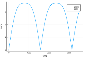
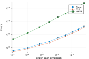
Figure 1: (a)Time evolution of $L^{2}$ error (semi-$\log_{10}$ scale) for NUFFT, ESR, and Strang for 3D transport problem with grids $64^{3}$ and step size $\Delta t=0.3$; (b) CPU time for NUFFT, ESR and Strang of after running $100$ steps.

4D transport equation
We consider now the case $n=4$ where the matrix $M$ in (5) is given by

$$M=\begin{pmatrix}0&1&-1.5&-3\\ -1&0&2&1\\ 1.5&-2&0&0\\ 3&-1&0&0\end{pmatrix}.$$

The domain is defined by $R=5$ and the initial value is

$$f_{0}({\mathbf{x}})=\left(\frac{2}{\pi}\right)^{4}e^{-{|\mathbf{x}|}^{2}}.$$ (13)

Since the direct 4D semi-Lagrangian method would be too costly, we compare here the Strang directional splitting and the new method ESR. From Proposition  1, we define the ESR method by

$$e^{\Delta tM{\mathbf{x}}\cdot\nabla}=e^{\Delta t(y^{(\ell)}\cdot{\mathbf{x}})\partial_{x_{2}}}\left(e^{\Delta t(y^{(1)}\cdot{\mathbf{x}})\partial_{x_{1}}}e^{\Delta t(y^{(3)}\cdot{\mathbf{x}})\partial_{x_{3}}}e^{\Delta t(y^{(4)}\cdot{\mathbf{x}})\partial_{x_{4}}}\right)e^{\Delta t(y^{(r)}\cdot{\mathbf{x}})\partial_{x_{2}}},$$

whose coefficients are given by ($\Delta t=0.05$ here)

$$y^{(\ell)}\simeq\begin{pmatrix}7.239003439520237\\ 0\\ 0.114915806141710\\ 5.520828626111525\end{pmatrix},\;\;y^{(r)}\simeq\begin{pmatrix}-7.124076298503538\\ 0\\ -1.578152453772511\\ -5.445447353939971\end{pmatrix},$$

and

$$y^{(1)}\!\simeq\!\begin{pmatrix}0\\ -0.843365270467026\\ 1.542035786578973\\ 3.239936743553417\end{pmatrix}\!\!,\;y^{(3)}\!\simeq\!\!\begin{pmatrix}-2.171812638482090\\ 1.937050589058292\\ 0\\ -0.368205582274782\end{pmatrix}\!\!,\;\;y^{(4)}\!\simeq\!\!\begin{pmatrix}-3.333162655369549\\ 0.915289658696578\\ 0.087822505478295\\ 0\end{pmatrix}\!\!.$$

In the following numerical results, the space grid has $N=47$ points per direction and the final computation time is $t=30$ for the two methods. In Figure 2, the time evolution (in semi-$\log$ scale) of the $L^{2}$ error defined in (12) is plotted for the Strang method: the error grows up to $10^{-4}$ whereas the error for ESR is about $10^{-11}$. Moreover, some contour plots are also presented in Figure 2: the two-dimensional quantity $f(t,x_{1},x_{2},x_{3}=-0.9574,x_{4}=-0.9574)$ for $t=0$ and $t=30$ is displayed for ESR and Strang. One can observe that the Strang method has large errors which is partly due to the wrong angular velocity. Let us remark that even if pseudo-spectral method have been chosen here to make the error close to machine precision, alternative reconstruction methods can also be chosen such as high order interpolation methods (see [11]). Regarding the complexity, only $n+1=5$ shears are required in the exact splitting for each time step whereas $2n-1=7$ shears are needed for the Strang splitting.

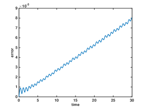
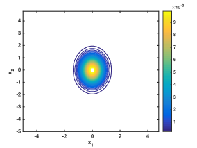
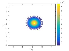
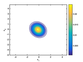
Figure 2: (a) Time evolution of $L^{2}$ error (semi-$\log_{10}$ scale of Strang; (b) Initial contour plot of $f(t=0,x_{1},x_{2},-0.9574,-0.9574)$; (c) Contour plot of $f(t=30,x_{1},x_{2},-0.9574,-0.9574)$ by ESR; (d) Contour plot of $f(t=30,x_{1},x_{2},-0.9574,-0.9574)$ by Strang.

4 Application to Fokker-Planck equations

In this section, we are interested in Fokker-Planck type equations which can be used to describe particles system (in plasma physics or astrophysics). The unknown is a distribution function of particles $f(t,x,v)\in\mathbb{R}^{+}$ with the time $t\geq 0$ the space $x\in\mathbb{R}$ and velocity $v\in\mathbb{R}$. We will focus on two examples which contains a free transport part in $x$ and an operator (related to collisional terms) which only acts on the $v$ direction. The first example is the Kramer-Fokker-Planck equation (see [18, 17, 15] for some mathematical and numerical aspects)

$$\partial_{t}f+v^{2}f-\partial_{v}^{2}f+v\partial_{x}f=0,\;\;f(t=0,x,v)=f_{0}(x,v).$$ (KFP)

The second example is the Fokker-Planck equation (see [19, 17, 15] for some mathematical and numerical aspects)

$$\partial_{t}f+v\partial_{x}f-\partial_{v}^{2}f-\partial_{v}(vf)=0,\;\;f(t=0,x,v)=f_{0}(x,v).$$ (FP)

For these two examples which enter in the class of inhomogeneous quadratic equations, exact splittings will be recalled from [8] and numerical results will be given.

4.1 Presentation of the exact splittings

For the Kramer-Fokker-Planck equation, the symbol is $p(x,v,\xi,\eta)=v^{2}+\eta^{2}+iv\xi$, and it writes $p(x,v,\xi,\eta)=iv\xi+\eta^{2}-iv\eta-\frac{1}{2}$ for the Fokker-Planck equation, where $\xi$ (resp. $\eta$) denotes the Fourier variable of $x$ (resp. $v$). We can see that for both cases, it is a polynomial function of degree $2$ and according to [8], the solution can be split exactly into simple flows. More precisely, for KFP, we have the following exact splitting formula

$$\forall t\geq 0,\ e^{-t(v^{2}-\partial_{v}^{2}+v\partial_{x})}=e^{-\frac{1}{2}\tanh t\ v^{2}}e^{\nabla\cdot(A^{KFP}_{t}\nabla)}e^{-\tanh t\ v\partial_{x}}e^{-\frac{1}{2}\tanh t\ v^{2}},$$ (14)

with $\nabla=(\partial_{x},\partial_{v})$ and where $A_{t}$ is the following nonnegative matrix defined by

$$A^{KFP}_{t}=\frac{1}{2}\begin{pmatrix}\frac{1}{2}\left(t-\tanh t(1-\sinh(t)^{2})\right)&\sinh^{2}t\\ \sinh^{2}t&\sinh 2t\end{pmatrix}.$$ (15)

For FP, we have the exact splitting formula

$$e^{-t(v\partial_{x}-\partial_{v}^{2}-\partial_{v}v)}=e^{t/2}e^{-(e^{t}-1)v\partial_{x}}e^{\nabla\cdot(A^{FP}_{t}\nabla)}e^{i\alpha_{t}\partial_{v}^{2}}e^{-i\beta_{t}v^{2}}e^{-i\beta_{t}\partial_{v}^{2}}e^{i\alpha_{t}v^{2}},$$ (16)

where $\alpha_{t}=\frac{1}{2}\sqrt{(1-e^{-t})e^{-t}}$, $\beta_{t}=\frac{1}{2}\sqrt{e^{t}-1}$, and $A^{FP}_{t}$ is the positive following matrix (see [1]) defined by

$$A^{FP}_{t}=\frac{1}{2}\begin{pmatrix}e^{2t}+2t+3-4e^{t}&-4\sinh^{2}(t/2)\\ -4\sinh^{2}(t/2)&1-e^{-2t}\end{pmatrix}.$$

Below, we detail a bit the link between splitting for PDE and finite dimensional Hamiltonian systems for the KFP case. Following [8], the exact splitting (14) is equivalent to prove the following equality between matrices

$$e^{-2itJQ}=e^{-2itJQ_{1}}e^{-2itJQ_{2}}e^{-2itJQ_{3}}e^{-2itJQ_{1}},$$ (17)

where $J$ is the symplectic $4$x$4$ matrix, $Q,Q_{i}\in\mathrm{S}_{4}(\mathbb{C})$ ($i=1,2,3$) are the matrices corresponding to the quadratic form $q,q_{i}$ ($i=1,2,3$) defining the operators involving in the exact splitting (14). Indeed, the quadratic form $q$ associated to the quadratic operator $q^{w}:=v^{2}-\partial_{v}^{2}+v\partial_{x}$ is $q(X)=\mskip 1.0mu\prescript{\smash{\mathrm{t}\mkern-3.0mu}}{}{\mathstrut X}QX$ with $X=(x,v,\xi,\eta)$ and where $Q$ is given by

$$Q=\begin{pmatrix}0&0&0&0\\ 0&1&i/2&0\\ 0&i/2&0&0\\ 0&0&0&1\end{pmatrix}.$$

Let us define the other quadratic form involved in (14): $q_{1}(X)=\frac{\tanh t}{t}v^{2}=\mskip 1.0mu\prescript{\smash{\mathrm{t}\mkern-3.0mu}}{}{\mathstrut X}Q_{1}X,\ q_{2}(X)=\mskip 1.0mu\prescript{\smash{\mathrm{t}\mkern-3.0mu}}{}{\mathstrut X}Q_{2}X,\ q_{3}=i\frac{\tanh t}{t}v\xi=\mskip 1.0mu\prescript{\smash{\mathrm{t}\mkern-3.0mu}}{}{\mathstrut X}Q_{3}X$ where

$$Q_{1}=\frac{\tanh t}{t}\begin{pmatrix}0&0&0&0\\ 0&1&0&0\\ 0&0&0&0\\ 0&0&0&0\end{pmatrix},\;Q_{2}=\frac{1}{t}\begin{pmatrix}{\bf 0}_{2}&{\bf 0}_{2}\\ {\bf 0}_{2}&A_{t}^{KFP}\end{pmatrix},\;Q_{3}=\frac{\tanh t}{t}\begin{pmatrix}0&0&0&0\\ 0&0&i/2&0\\ 0&i/2&0&0\\ 0&0&0&0\end{pmatrix},$$

where ${\bf 0}_{2}$ is the zero $2$x$2$ matrix and $A_{t}^{KFP}$ is given by (15).

Let us now focus on the FP case. From Theorem 2.1 in [8], we have

$$e^{-t(v\partial_{x}-\partial_{v}^{2}-\partial_{v}v)}=e^{-t(iv\xi+\eta^{2}-iv\eta-\frac{1}{2})^{w}}=e^{t/2}e^{-t(\eta^{2}+i(v\xi-v\eta))^{w}},$$

so that the $e^{-t(\eta^{2}+i(v\xi-v\eta))^{w}}$ only involves homogeneous quadratic form and can be split as (16) and then can be checked as in the KFP case.

4.2 Numerical results

In this section, numerical simulations are performed using the above exact splittings to illustrate the exponential decay to equilibrium property and regularizing effects. Let us remark that since the Fokker-Planck and Krammer-Fokker-Planck operators are homogeneous with respect to the space variable $x$, we do not have to consider localized functions in this direction and we can thus periodic functions in this direction. The domain is truncated to $(x,v)\in[-R_{1},R_{1}]\times[-R_{2},R_{2}]$ and the number of points is denoted by $N_{1}$ (resp. $N_{2}$) to sample the $x$-direction (resp. the $v$-direction).

Fokker-Planck equation
For the FP equation, we aim at checking an important property that the solution converges to the equilibrium state exponentially with time (see [15]). The domain is taken as $R_{1}=\pi$ and $R_{2}=7$ (so that $(x,v)\in[-\pi,\pi]\times[-7,7]$) and the initial function is

$$f_{0}(x,v)=\frac{1}{\sqrt{2\pi}}\exp(-v^{2}/2)\left(1+0.5\sin(x)\cos(\frac{\pi}{7}v)\right).$$

We will be interested in the time evolution of the entropy which is defined by

$$\mathcal{F}(t)=\int_{0}^{L}\int_{-\infty}^{\infty}\frac{(f(t,x,v)-\mu(v))^{2}}{\mu(v)}\mathrm{d}v\mathrm{d}x,$$ (18)

with $\mu(v)=\frac{1}{\sqrt{2\pi}}e^{-\frac{v^{2}}{2}}$.

The numerical parameters are $N_{1}=27$, $N_{2}=181$ and the time step is $\Delta t=0.1$ whereas the simulation is ended at $t=20$. In Figure 3, the distribution function is plotted at the initial and the ending time and we can observe the relaxation towards the Maxwellian profile. This is more quantitatively shown in Figure 3-(c) where the time history of entropy (18) is plotted (semi-$\log_{10}$ scale). Indeed, the exponential decay is clearly observed, the rate of which is equal to $-1.99$ (red straight line) which is good agreement with [15].

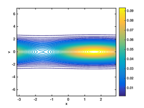
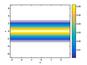
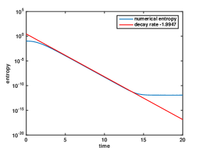
Figure 3: (a) Initial distribution function $f(t=0,x,v)$; (b) distribution function at $t=20$: $f(t=20,x,v)$; (c) time evolution of the entropy given by (18).

Kramer-Fokker-Planck equation
Now, we are interested in the numerical simulation of the KFP equation. The domain is chosen with $R_{1}=4$ and $R_{2}=15$ (so that $(x,v)\in[-4,4]\times[-15,15]$). In the following experiments, we have considered $N_{1}=N_{2}=199$.

First, in Figure 5, we plot the $L^{2}$ error in $x$ and $v$ (in $\log_{10}-\log_{10}$ scale) of the following formula

$$e^{-\Delta t(v^{2}-\partial_{v}^{2}+v\partial_{x})}f_{0}(x,v)-e^{-\Delta t/2(v^{2}-\partial_{v}^{2}+v\partial_{x})}e^{-\Delta t/2(v^{2}-\partial_{v}^{2}+v\partial_{x})}f_{0}(x,v)$$ (19)

using different time steps and where the initial data is smooth enough (a Maxwellian is considered here). Two different methods are used to compute the quantity $e^{-t(v^{2}-\partial_{v}^{2}+v\partial_{x})}f_{0}(x,v)$: the exact splitting (14) and a Strang operator splitting. First, we observe that the exact splitting gives an error at the machine precision level whereas we obtain an error of ${\cal O}(\Delta t^{3})$ which corresponds the local error of the Strang method.

Then, our goal is to illustrate a result from [1] in which the authors proved that the evolution operator of KFP has regularizing effects. To do so, the initial condition is chosen as random values (discrete $L^{1}$ norm is 1) and the step size is $\Delta t=0.1$. In Figure 4, the distribution function is plotted for different times: $t=0,0.2,1,100$. We observe that starting from a random initial value, the numerical solution becomes smoother and smoother as time increases. Moreover, it can be proved that the solution is exponentially decreasing in time towards zero. This is illustrated in Figure 6 where we plot the time history $L^{2}$ norm (in $x$ and $v$) of $f$ in semi-$\log_{10}$ scale.

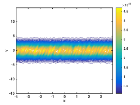
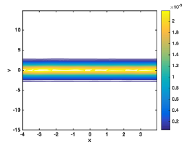
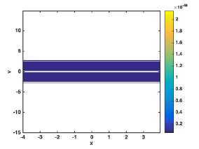
Figure 4: Time evolution of the distribution function $f$ (a) $t=0$; (b) $t=0.2$; (c) $t=1$; (d) $t=100$.

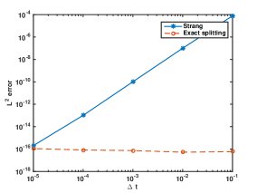
Figure 5: $L^{2}$ error ($\log_{10}-\log_{10}$ scale) of the formula (19) with different time step size $\Delta t$.

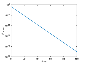
Figure 6: Time evolution of the $L^{2}$ norm (in $x$ and $v$) of $f$ in semi-$\log_{10}$ scale.

5 Application to Schrödinger equations

In this section, we consider Schrödinger type equations. First, the Schrödinger in the presence of an external electromagnetic field is an important model in computational quantum mechanics. The second model is the Gross-Pitaevskii equation with angular momentum rotation which is widely used to describe Bose Einstein condensate at low temperature. We refer to [27, 12, 5, 6, 7] for more details on these models.

Then, we consider the following linear Schrödinger equation (with a rotation term and a quadratic external potential) of unknown $\psi({\bf x},t)\in\mathbb{C}$ with ${\mathbf{x}}\in\mathbb{R}^{n},\ t\in\mathbb{R}_{+}$

$$i\frac{\partial\psi({\bf x},t)}{\partial t}=-\frac{1}{2}\Delta\psi({\bf x},t)-i({B}{\bf x})\cdot\nabla\psi({\bf x},t)+V({\bf x})\psi({\bf x},t),\;\;\psi({\mathbf{x}},t=0)=\psi_{0}({\mathbf{x}}),$$ (QM)

where $n\in\mathbb{N}^{*}$, $B\in A_{n}(\mathbb{R})$ is a skew symmetric matrix of size $n$ and $V:\mathbb{R}^{n}\to\mathbb{R}$ is a quadratic potential. According to the previous framework, this model is an inhomogeneous quadratic PDEs since it can be represented by the following symbol

$$p(X)=i\frac{|\boldsymbol{\xi}|^{2}}{2}+iB{\mathbf{x}}\cdot{\boldsymbol{\xi}}+iV({\mathbf{x}}),\;\;X=({\mathbf{x}},\boldsymbol{\xi})\in\mathbb{R}^{2n}.$$ (20)

In the sequel, an exact splitting is presented for which the construction will be detailed. Then, an extension to nonlinear and non quadratic Schrödinger equations are discussed. This section will be ended by several numerical results that will be compared to different strategies from the literature to illustrate the efficiency of our approach.

5.1 Presentation of the exact splitting

We present an exact splitting method for (QM) which has been introduced in [8].

Theorem 5.1.

There exists some quadratic forms $v_{t}^{(r)},a_{t}$ on $\mathbb{R}^{n}$, a strictly upper triangular matrix $U_{t}\in M_{n}(\mathbb{R})$, a strictly lower triangular matrix $L_{t}\in M_{n}(\mathbb{R})$ and a diagonal quadratic form $v_{t}^{(\ell)}$ on $\mathbb{R}^{n}$, all depending analytically on $t\in(-t_{0},t_{0})$ for some $t_{0}>0$, such that for all $t\in(-t_{0},t_{0})$ we have

$$e^{it(\Delta/2-V({\mathbf{x}}))-tB{\mathbf{x}}\cdot\nabla}=e^{-itv^{(\ell)}_{t}({\mathbf{x}})}\left(\prod_{j=1}^{n-1}e^{-t(U_{t}{\mathbf{x}})_{j}\partial_{x_{j}}}\right)e^{ita_{t}(\nabla)}\left(\prod_{j=2}^{n}e^{-t(L_{t}{\mathbf{x}})_{j}\partial_{x_{j}}}\right)e^{-itv^{(r)}_{t}({\mathbf{x}})}$$ (21)

where $a_{t}(\nabla)$ denotes the Fourier multiplier of symbol $-a_{t}({\boldsymbol{\xi}})$ and $(U_{t}{\mathbf{x}})_{j}$ (resp. $(L_{t}{\mathbf{x}})_{j}$) the $j^{\mathrm{st}}$ coordinate of $U_{t}{\mathbf{x}}$ (resp. $L_{t}{\mathbf{x}}$).

Let us detail the steps of this splitting to emphasize the fact that, due the triangular structure of the matrices $L_{t}$ and $U_{t}$, only $2n$ FFT calls are required.

• From $e^{-itv^{(r)}_{t}({\mathbf{x}})}$ to $e^{-t(L_{t}{\mathbf{x}})_{n}\partial_{x_{n}}}$, we need a FFT in $x_{n}$ direction;

• From $e^{-t(L_{t}{\mathbf{x}})_{j}\partial_{x_{j}}}$ to $e^{-t(L_{t}{\mathbf{x}})_{j-1}\partial_{x_{j-1}}},\ j\in\llbracket 3,n\rrbracket$, as $L_{t}$ is a strictly lower triangular matrix, $(L_{t}{\mathbf{x}})_{j}$ only depends on $x_{i},\,i\in\llbracket 1,j-1\rrbracket$, then we only need a FFT in $x_{j-1}$ direction.

• From $e^{-t(L_{t}{\mathbf{x}})_{2}\partial_{x_{2}}}$ to $e^{ita_{t}(\nabla)}$, we need a FFT in $x_{1}$ direction.

• From $e^{ita_{t}(\nabla)}$ to $e^{-t(U_{t}{\mathbf{x}})_{n-1}\partial_{x_{n-1}}}$, we need an inverse FFT in $x_{n}$ direction;

• From $e^{-t(U_{t}{\mathbf{x}})_{j}\partial_{x_{j}}}$ to $e^{-t(U_{t}{\mathbf{x}})_{j-1}\partial_{x_{j-1}}},\ j\in\llbracket 2,n-1\rrbracket$, because $U_{t}$ is a strictly upper triangular matrix, $(U_{t}{\mathbf{x}})_{j-1}$ only depends on $x_{i},\,i\in\llbracket j,n\rrbracket$, we only need an inverse FFT in $x_{j}$ direction.

• From $e^{-t(U_{t}{\mathbf{x}})_{1}\partial_{x_{1}}}$ to $e^{-itv^{(\ell)}_{t}({\mathbf{x}})}$, we need an inverse FFT in $x_{1}$ direction.

To sum up, this new method only needs $2n$ FFT (or inverse FFT) calls,

Below, we detail a bit the link between splitting for the Schrödinger equations and finite dimensional Hamiltonian systems. Following [8], the exact splitting (21) is equivalent to prove an equality at the level of matrices. Indeed, from Hörmander [21], there exists a morphism between the Hamiltonian flow of the following linear ODE $\dot{X}=-iJ\nabla p(X)$ and $e^{-p^{w}}$ (up to one sign), where $J$ is the symplectic $2n$ matrix. So we can check the following exact splitting at the linear ODE level for (21):

$$e^{-2itJQ}=e^{-2itJV^{(\ell)}}\left({\prod_{j=1}^{n-1}}e^{-2itJU^{(j)}}\right)e^{-2itJA}\left({\prod_{j=2}^{n}}e^{-2itJL^{(j)}}\right)e^{-2itJV^{(r)}},$$ (22)

where $Q,V^{(\ell)},U^{(j)},L^{(j)},V^{(r)}$ are symmetric matrices of the quadratic forms (symbols) of the following operators $iv^{(\ell)}_{t}({\mathbf{x}}),i(U_{t}{\mathbf{x}})_{j}\partial_{x_{j}},-iA_{t}(\nabla),i(L_{t}{\mathbf{x}})_{j}\partial_{x_{j}},iv^{(r)}_{t}({\mathbf{x}})$ respectively.

5.2 Practical construction of the splittings

In this subsection, the iteration methods giving the coefficients of two above exact splittings are given. The proof for Theorem 5.1 is based on the implicit function theorem which gives a practical way to construct the exact splitting. Indeed, it furnishes an iteration method which is presented below. We refer to [8] for more details.

In this context, the iterative method giving the coefficients of the exact splitting can be made much more explicit. Indeed, identifying a quadratic form with its symmetric matrix in order we define, if $t$ is small enough, we define, by induction, the following sequences

$$\left\{\begin{array}[]{lll}A_{t,k+1}&=&A_{t,k}+I_{n}/2-\widetilde{A}_{t,k}\\ L_{t,k+1}&=&L_{t,k}+L-\widetilde{L}_{t,k}\\ U_{t,k+1}&=&U_{t,k}+U-\widetilde{U}_{t,k}\\ V_{t,k+1}^{(m)}&=&V_{t,k}^{(m)}+V-\widetilde{V}_{t,k}^{(m)}+\frac{t}{2}[D_{t,k},B]+\frac{t^{2}}{2}D_{t,k}^{2}\end{array}\right.$$

where $(A_{t,0},L_{t,0}+U_{t,0},V_{t,0}^{(m)})=(I_{n}/2,B,V)$, $L+U=B$ and

$$\begin{pmatrix}2\widetilde{V}_{t,k}^{(m)}&\mskip 1.0mu\prescript{\smash{\mathrm{t}\mkern-3.0mu}}{}{\mathstrut\widetilde{L}_{t,k}}+\mskip 1.0mu\prescript{\smash{\mathrm{t}\mkern-3.0mu}}{}{\mathstrut\widetilde{U}_{t,k}}+tD_{t,k}\\ \widetilde{L}_{t,k}+\widetilde{U}_{t,k}+tD_{t,k}&2\widetilde{A}_{t,k}\\ \end{pmatrix}=-t^{-1}J\log(P_{t,k})$$

and

$$P_{t,k}=\left[\prod_{j=1}^{n-1}\begin{pmatrix}I_{n}+tU_{t,k}^{(j)}&\\ &I_{n}-t\mskip 1.0mu\prescript{\smash{\mathrm{t}\mkern-3.0mu}}{}{\mathstrut U_{t,k}^{(j)}}\end{pmatrix}\right]\begin{pmatrix}I_{n}&2tA_{t,k}\\ &I_{n}\end{pmatrix}\left[\prod_{j=2}^{n}\begin{pmatrix}I_{n}+tL_{t,k}^{(j)}&\\ &I_{n}-t\mskip 1.0mu\prescript{\smash{\mathrm{t}\mkern-3.0mu}}{}{\mathstrut L_{t,k}^{(j)}}\end{pmatrix}\right]\\ \times\begin{pmatrix}I_{n}&\\ -2tV_{t,k}^{(m)}&I_{n}\end{pmatrix}$$

with $L_{t,k}^{(j)}=(e_{j}\otimes e_{j})L_{t,k}$, $U_{t,k}^{(j)}=(e_{j}\otimes e_{j})U_{t,k}$ and $(e_{1},\dots,e_{n})$ the canonical basis of $\mathbb{R}^{n}$.

As previously, one can prove that the sequence $(\widetilde{A}_{t,k},\widetilde{L}_{t,k},\widetilde{U}_{t,k},-\frac{t}{2}D_{t,k},V_{t,k}^{(m)}+\frac{1}{2}D_{t,k})$ generated by this induction converges towards the elements which define the splitting in 5.1, i.e.

$$|A_{t}-\widetilde{A}_{t,k}|+|L_{t}-\widetilde{L}_{t,k}|+|U_{t}-\widetilde{U}_{t,k}|+|V_{t}^{(\ell)}+\frac{1}{2}D_{t,k}|+|V_{t}^{(r)}-V_{t,k}^{(m)}-\frac{1}{2}D_{t,k}|\leq\left(\frac{t}{\tau_{0}}\right)^{k}.$$

as soon as $t$ is small enough ($0<|t|<\tau_{0}$ for a given $\tau_{0}>0$).

5.3 Extension to more general Schrödinger equations

Before presenting some numerical results, some time discretizations based on the previous exact splitting are proposed here in order to tackle more general Schrödinger equations. Keeping the same notations $\psi({\bf x},t)\in\mathbb{C}$ for the unknown (${\bf x}\in\mathbb{R}^{n}$ and $t\geq 0$), we then consider the following Schrödinger equation to illustrate our strategy

$$i\frac{\partial\psi({\bf x},t)}{\partial t}=-\frac{1}{2}\Delta\psi({\bf x},t)-i({B}{\bf x})\cdot\nabla\psi({\bf x},t)+V({\bf x})\psi({\bf x},t)+f({\bf x},|\psi|^{2})\psi({\bf x},t),$$ (23)

where $f$ is a real valued function, ${B}\in A_{n}(\mathbb{R})$ is a skew symmetric matrix of size $n$, and $V({\bf x}):\mathbb{R}^{n}\to\mathbb{R}$ is a real valued quadratic potential. Some well known examples can be given in the case $n=2,3$

• $f({\bf x},|\psi|^{2})=\beta|\psi|^{2}$ ($\beta\in\mathbb{R}$) and $({B{\mathbf{x}}})\cdot\nabla\psi=\Omega(x_{2}\partial_{x_{1}}-x_{1}\partial_{x_{2}})\psi(\Omega\in\mathbb{R})$. In this case, (23) is the so-called Gross–Pitaevskii equation (GPE) with an angular momentum rotation term (see [6, 7]).

• $f({\bf x},|\psi|^{2})=V_{nq}({\bf x})$ where $V_{nq}({\bf x})$ denotes a non-quadratic potential and $V({\bf x})=\frac{1}{2}|{B{\mathbf{x}}}|^{2}$. In this case, (23) is the so-called magnetic Schrödinger equation (see [23, 12]).

On can show that (23) has the following two conserved quantities,

$$\text{(mass)}\quad M(t)=\int_{\mathbb{R}^{n}}|\psi({\bf x},t)|^{2}\mathrm{d}{\bf x},$$ (24)

$$\text{(energy)}\quad E(t)=\int_{\mathbb{R}^{n}}\Big{[}\frac{1}{2}|\nabla\psi|^{2}+V|\psi|^{2}+f({\bf x},|\psi|^{2})|\psi|^{2}-\text{Re}(i({B}{\bf x})\cdot\nabla\psi\,\psi^{*})\Big{]}\mathrm{d}{\bf x},$$

where $f^{*}$ and $\text{Re}(f)$ denote the conjugate and real part of the function $f$ respectively.

From the exact splitting presented above, we deduce a new splitting for (23). This splitting is based on Strang composition of the quadratic and the non-quadratic parts. Indeed, we first rewrite (23) as

$$i\partial_{t}\psi=-p^{w}\psi+f({\bf x},|\psi|^{2})\psi,$$

where $-p^{w}\psi:=-\frac{1}{2}\Delta\psi-i({B}{\bf x})\cdot\nabla\psi+V({\bf x})\psi$ denotes the quadratic part (in the sense of Section 2) and $f({\bf x},|\psi|^{2})\psi$ denotes the non quadratic part (which can be nonlinear). Based on this formulation and on the fact that exact splitting have been derived for the quadratic part, we then propose the following splitting (ESQM method)

$$(\psi({\bf x},t_{n})\approx)\psi^{n}({\mathbf{x}})\ \ =\left(e^{-i\frac{\Delta t}{2}f({\mathbf{x}},|\psi|^{2})}e^{-i\Delta tp^{w}}e^{-i\frac{\Delta t}{2}f({\mathbf{x}},|\psi|^{2})}\right)^{n}\psi_{0}({\mathbf{x}})$$ (25)

where the computation of $e^{-i\Delta tp^{w}}$ is done using (21). Let us remark that in this Strang based splitting, each part can be solved exactly in time and high order composition methods can be easily used to derive arbitrary high order time integrator (see [16]). It can be shown that $\|\psi^{n}\|_{\ell^{2}}$ is preserved by the numerical schemes proposed here. In Algorithm 1, we detail the different steps of the exact splitting (25) involving the pseudo-spectral discretization in dimension $3$.

Algorithm 1 Pseudo-spectral method for ESQM (25)

0:  $\psi^{0}=\psi^{0}_{|\mathbb{G}_{1}\times\mathbb{G}_{2}\times\mathbb{G}_{3}}$

1:  for $n=0$ to $n_{final}-1$ do

2:     $\psi^{(1)}=e^{-i\Delta t/2\;f(g,|\psi_{g}^{n}|^{2})}\psi^{n}$

3:     $\psi^{(2)}=e^{-i\Delta tV^{(r)}_{\Delta t}(g)}\psi^{(1)}$

4:     ${\psi}^{(3)}=e^{-i\Delta t\omega_{3}(L_{\Delta t,31}g_{1}+L_{\Delta t,32}g_{2})}\mathcal{F}_{3}\psi^{(2)}$

5:     ${\psi}^{(4)}=e^{-i\Delta t\omega_{2}L_{\Delta t,21}g_{1}}\mathcal{F}_{2}{\psi}^{(3)}$

6:     ${\psi}^{(5)}=e^{-i\Delta ta(\omega)}\mathcal{F}_{1}{\psi}^{(4)}$

7:     ${\psi}^{(6)}=e^{-i\Delta t\omega_{2}U_{\Delta t,23}g_{3}}\mathcal{F}^{-1}_{3}{\psi}^{(5)}$

8:     ${\psi}^{(7)}=e^{-i\Delta t\omega_{1}(U_{\Delta t,12}g_{2}+U_{\Delta t,13}g_{3})}\mathcal{F}^{-1}_{2}{\psi}^{(6)}$

9:     $\psi^{(8)}=e^{-i\Delta tV^{(r)}_{\Delta t}(g)}\mathcal{F}_{1}^{-1}{\psi}^{(7)}$

10:     $\psi^{n+1}=e^{-i{\Delta t/2}\;f(g,|\psi_{g}^{(8)}|^{2})}{\psi}^{(8)}$

11:  end for

11:  $\psi^{n_{final}}$

Remark 3.

Note that some optimizations can be performed in Algorithm 1 by noticing the following rearrangement

$$\begin{split}\psi^{n_{final}}&=\left(e^{-i\frac{\Delta t}{2}f({\mathbf{x}},|\psi|^{2})}e^{i\Delta t(-V({\mathbf{x}})+\frac{\Delta}{2}-B{\mathbf{x}}\cdot\nabla)}e^{-i\frac{\Delta t}{2}f({\mathbf{x}},|\psi|^{2})}\right)^{n_{final}}\psi^{0}\\ &=e^{-i\frac{\Delta t}{2}f({\mathbf{x}},|\psi|^{2})-i\Delta tV^{(\ell)}_{\Delta t}({\mathbf{x}})}e^{-t(U_{\Delta t}{\mathbf{x}})_{1}\partial_{x_{1}}}e^{-t(U_{\Delta t}{\mathbf{x}})_{2}\partial_{x_{2}}}e^{itA_{\Delta t}(\nabla)}e^{-\Delta t(L_{\Delta t}{\mathbf{x}})_{2}\partial_{x_{2}}}e^{-\Delta t(L_{t}{\mathbf{x}})_{3}\partial_{x_{3}}}\\ &\left(e^{-i{\Delta t}f({\mathbf{x}},|\psi|^{2})-i\Delta tV^{(\ell)}_{\Delta t}({\mathbf{x}})-i\Delta tV^{(r)}_{\Delta t}({\mathbf{x}})}e^{-\Delta t(U_{\Delta t}{\mathbf{x}})_{1}\partial_{x_{1}}}e^{-\Delta t(U_{\Delta t}{\mathbf{x}})_{2}\partial_{x_{2}}}e^{i\Delta tA_{\Delta t}(\nabla)}\right.\\ &\left.e^{-\Delta t(L_{\Delta t}{\mathbf{x}})_{2}\partial_{x_{2}}}e^{-\Delta t(L_{\Delta t}{\mathbf{x}})_{3}\partial_{x_{3}}}\right)^{n_{final}-1}e^{-i\Delta tV^{(r)}_{\Delta t}(\mathbf{x})-i\frac{\Delta t}{2}f({\mathbf{x}},|\psi|^{2})}\psi^{0}.\end{split}$$ (26)

5.4 Numerical results

This section is devoted to applications of exact splittings to the Schrödinger equations (23) both in the two and three dimensional cases. We show higher accuracy and efficiency of the exact splitting by comparing it to other usual numerical methods proposed in the literature [7].

As previously, the space discretization requires a truncated domain denoted by $[-R_{1},R_{1}]\times\dots\times[-R_{n},R_{n}]$. We will consider a uniform grid with $N_{j}$ points per direction so that the mesh size are $2R_{j}/N_{j}$.

5.4.1 2D Schrödinger equations

Firstly, we consider the application of the exact splitting in the two-dimensional case on the magnetic Schrödinger equation and on the rotating Gross-Pitaevskii equation.

2D magnetic Schrödinger equation
In this numerical experiment, the 2D magnetic Schrödinger equation is considered [23],

$$i\epsilon\partial_{t}\psi({\bf x},t)=-\frac{\epsilon^{2}}{2}\Delta\psi({\bf x},t)+i\epsilon{\bf A}\cdot\nabla\psi({\bf x},t)+\frac{1}{2}{|\bf A|}^{2}\psi({\bf x},t),$$ (27)

with $\epsilon=1/32$ and where ${\bf x}=(x_{1},x_{2})\in\mathbb{R}^{2}$, ${\bf A}=\frac{1}{2}\mskip 1.0mu\prescript{\smash{\mathrm{t}\mkern-3.0mu}}{}{\mathstrut(-x_{2},x_{1})}$. The initial condition is given by

$$\psi_{0}({\bf x})=e^{-20(x_{1}-0.05)^{2}-20(x_{2}-0.1)^{2}}e^{i\sin(x_{1})\sin(x_{2})/\epsilon}.$$

The numerical parameters are chosen as follows: $N_{1}=N_{2}=256$, $R_{1}=R_{2}=3\pi$ and $\Delta t=0.3$. We shall compare three different splittings:

• ESQM (see (25) with $f=0$ and (21)); this method is exact in time.

• ESR (see Appendix 6.1); this method is second order accurate in time.

• Strang (see Appendix 6.1); this method is second order accurate in time.

Let us remark that ESR and Strang are two operator splittings which differ from the treatment of the rotation part $\partial_{t}\psi={\bf A}\cdot\nabla\psi$. Indeed, this part is solved exactly in the ESR method (this is the reason why we used the same name as in Section 3) whereas a second order directional splitting is used to approximate it in the Strang method. We refer to Appendix 6.1 for the details. Let us now write the operators which define the exact splitting ESQM. From (21), we have

$$e^{i\epsilon\Delta t(\frac{\Delta}{2}-\frac{1}{2\epsilon^{2}}|{\mathbf{A}}|^{2})+\epsilon\Delta t{\frac{\mathbf{A}}{\epsilon}}\cdot\nabla}=e^{-\epsilon\Delta tv^{(\ell)}({\mathbf{x}})}e^{-\epsilon\Delta t(U_{\Delta t}{\mathbf{x}})_{1}\partial x_{1}}e^{i\epsilon\Delta ta(\nabla)}e^{-\epsilon\Delta t(L_{\Delta t}{\mathbf{x}})_{2}\partial_{x_{2}}}e^{-\epsilon\Delta tv^{(r)}({\mathbf{x}})},$$

where $v^{(\ell)}({\mathbf{x}})={\mathbf{x}}^{\mathrm{T}}V_{\Delta t}^{(\ell)}{\mathbf{x}},\;\;v^{(r)}({\mathbf{x}})={\mathbf{x}}^{\mathrm{T}}V_{\Delta t}^{(r)}{\mathbf{x}}$, and $a(\nabla)=\nabla\cdot(A_{\Delta t}\nabla)$, $V_{\Delta t}^{(\ell)},L_{\Delta t},U_{\Delta t},V_{\Delta t}^{(r)},A_{\Delta t}$ being $2$x$2$ matrices. The corresponding coefficients for ESQM are

$$A_{\Delta t}\simeq\begin{pmatrix}0.503532819405421&-0.074439184790650\\ -0.074439184790650&0.503784060194312\end{pmatrix},$$

$$L_{\Delta t}\simeq\begin{pmatrix}0&0\\ -16.121089926218119&0\end{pmatrix},\quad U_{\Delta t}\simeq\begin{pmatrix}0&15.761077688604765\\ 0&0\end{pmatrix},$$

$$V^{(\ell)}_{\Delta t}\simeq\begin{pmatrix}128.9687194097432&0\\ 0&-0.0000000000018\end{pmatrix},$$

$$V^{(r)}_{\Delta t}\simeq\begin{pmatrix}2.8800979009085&-19.0564313064080\\ -19.0564313064080&126.0886215088400\end{pmatrix}.$$

First of all, we show the contour plots of $|\psi({\bf x},t)|^{2}$ at the final time $t=300$ in Figure 7 for the three methods. Second, the time history energy error (defined by (LABEL:eq:invariant)) obtained by the three methods is presented on Figure 8. As (27) is a quadratic equation, by Theorem 5.1, the ESQM method gives the exact solution (if neglecting space error). From Figure 8, we can see that its energy error is at machine precision level, which is much smaller than the energy errors of Strang and ESR (for which the energy errors oscillate around a constant). Specifically, as the rotation velocity of Strang is not correct (see [9]), we can see in Figure 7 that the contour plot obtained by Strang is not good. For ESR, even if the rotation velocity is right and as such the shape of the solution has the correct orientation, some error are clearly observed.

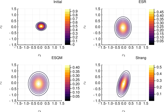
Figure 7: Contour plot of initial density, and the contour plots of ESQM, ESR and Strang splitting method at $t=300$ with $\Delta t=0.3$, $N_{1}=N_{2}=256$ and $\epsilon=\frac{1}{32}$ for 2D magnetic Schrödinger problem.

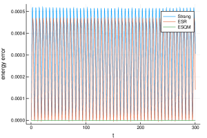
Figure 8: Time evolution of energy error of ESR, ESQM and Strang splitting method with $\Delta t=0.3$, $N_{1}=N_{2}=256$ and $\epsilon=\frac{1}{32}$ for 2D magnetic Schrödinger equation.

2D rotating Gross-Pitaevskii equation
We now consider the dynamics of rotating Bose-Einstein condensates, which is described by the macroscopic wave function $\psi({\bf x},t)$ (${\bf x}=(x_{1},x_{2})\in\mathbb{R}^{2},t\geq 0$) solution to the following rotating Gross-Pitaevskii equation (GPE) (see [6, 7])

$${i}\partial_{t}\psi({\bf x},t)=-\frac{1}{2}\Delta\psi({\bf x},t)+V({\bf x})\psi({\bf x},t)+\beta|\psi|^{2}\psi({\bf x},t)-\Omega L_{x_{3}}\psi({\bf x},t),\;\;\;\psi({\bf x},0)=\psi_{0}({\bf x})$$ (28)

where $L_{x_{3}}=-i(x_{1}\partial_{x_{2}}-x_{2}\partial_{x_{1}})$ is the $x_{3}$-component of the angular momentum, $\Omega$ is the angular speed of the laser beam, $\beta$ is a constant characterizing the particle interactions and $V({\bf x})$ denotes the external harmonic oscillator potential

$$V({\bf x})=\frac{1}{2}(\gamma_{x_{1}}^{2}x_{1}^{2}+\gamma_{x_{2}}^{2}x_{2}^{2}),$$ (29)

with constants $\gamma_{x_{1}}>0$ and $\gamma_{x_{2}}>0$.

In addition to the mass and energy preservations (LABEL:eq:invariant), the expectation of angular momentum is also conserved when $\gamma_{x_{1}}=\gamma_{x_{2}}$

$$Lz(t):=\int_{\mathbb{R}^{2}}\psi^{*}({\bf x},t)L_{x_{3}}\psi({\bf x},t)d{\bf x}=Lz(0).$$ (30)

We are also interested in the time evolution of condensate widths and mass center defined as follows,

$$\text{condensate widths}:\,S_{\alpha}(t)=\sqrt{\int_{\mathbb{R}^{2}}\alpha^{2}|\psi({\bf x},t)|^{2}d{\bf x}},\quad\alpha=x_{1},x_{2},$$ (31)

$$\text{mass center}:{\bf x}_{c}(t)=\int_{\mathbb{R}^{2}}{\bf x}|\psi({\bf x},t)|^{2}d{\bf x}.$$

For the two dimensional rotating GPE (LABEL:eq:gpe), our first numerical test is the so-called dynamics of a stationary state with a shifted center [6]. We take $\gamma_{x_{1}}=\gamma_{x_{2}}=1,\beta=100$ in (LABEL:eq:gpe) and the initial condition is taken as

$$\psi_{0}({\bf x})=\phi_{e}({\bf x}-{\bf x}_{0}),$$

where $\phi_{e}({\bf x})$ is a ground state computed numerically from [29] and ${\bf x}_{0}=\mskip 1.0mu\prescript{\smash{\mathrm{t}\mkern-3.0mu}}{}{\mathstrut(1,1)}$. The numerical parameters are chosen as follows: $\Delta t=0.001$ and the spatial domain $[-8,8]^{2}$ is discretized using $N_{1}=N_{2}=256$ points.

As in the magnetic Schrödinger case, we will consider the following three methods to approximate (LABEL:eq:gpe)

• ESQM (see (25) with $f({\bf x},|\psi|^{2})=\beta|\psi|^{2}$ and (21)); this method is second order accurate in time.

• ESR (see Appendix 6.2.1); this method is second order accurate in time.

• BW from [6] (see Appendix 6.2.2); this method is second order accurate in time.

Concerning ESQM, we then have to define from (21) how the quadratic part $p^{w}:=(i/2)\Delta-\Omega L_{x_{3}}-iV({\mathbf{x}})$ of the nonlinear equation (LABEL:eq:gpe) is split. This is done as follows (the two cases $\Omega=-0.5$ and $\Omega=0$ are considered)

$$e^{i\Delta tp^{w}}=e^{-\Delta tv^{(\ell)}({\mathbf{x}})}e^{-\Delta t(U_{\Delta t}{\mathbf{x}})_{1}\partial_{x_{1}}}e^{i\Delta ta(\nabla)}e^{-\Delta t(L_{\Delta t}{\mathbf{x}})_{2}\partial_{x_{2}}}e^{-\Delta tv^{(r)}({\mathbf{x}})},$$

where $v^{(\ell)}({\mathbf{x}})={\mathbf{x}}^{\mathrm{T}}V_{\Delta t}^{(\ell)}{\mathbf{x}},\;\;v^{(r)}({\mathbf{x}})={\mathbf{x}}^{\mathrm{T}}V_{\Delta t}^{(r)}{\mathbf{x}}$, and $a(\nabla)=\nabla\cdot(A_{\Delta t}\nabla)$, $V_{\Delta t}^{(\ell)},L_{\Delta t},U_{\Delta t},V_{\Delta t}^{(r)},A_{\Delta t}$ being $2$x$2$ matrices. In the case $\Omega=-0.5$, we have

$$A_{\Delta t}\simeq\begin{pmatrix}0.499999979166481&0.000249999948070\\ 0.000249999948070&0.499999979166811\end{pmatrix},$$

$$L_{\Delta t}\simeq\begin{pmatrix}0&0\\ 0.500000041666386&0\end{pmatrix},\quad U_{\Delta t}\simeq\begin{pmatrix}0&-0.499999916666976\\ 0&0\end{pmatrix},$$

$$V^{(\ell)}_{\Delta t}\simeq\begin{pmatrix}0.312500037673140&0\\ 0&0.187500011883192\end{pmatrix},$$

$$V^{(r)}_{\Delta t}\simeq\begin{pmatrix}0.187500043056181&0.000062500002332\\ 0.000062500002332&0.312500006345821\end{pmatrix}.$$

and in the case $\Omega=0$, we have

$$A_{\Delta t}\simeq\begin{pmatrix}0.499999916666670&0\\ 0&0.499999916666676\end{pmatrix},$$

$$L_{\Delta t}\simeq\begin{pmatrix}0&0\\ 0&0\end{pmatrix},\quad U_{\Delta t}\simeq\begin{pmatrix}0&0\\ 0&0\end{pmatrix},$$

$$V^{(\ell)}_{\Delta t}\simeq\begin{pmatrix}0.250000020830132&0\\ 0&0.250000020802363\end{pmatrix},$$

$$V^{(r)}_{\Delta t}\simeq\begin{pmatrix}0.250000020836539&0\\ 0&0.250000020864292\end{pmatrix}.$$

We first validate our ESQM approach by plotting the time history of mass center and condensate widths (31), and angular momentum expectation (30) in Figure 9. From [6], the mass center is known to be periodic, and the period is equal to $2\pi$ (resp. $4\pi$) when $\Omega=0$ (resp. $\Omega=-0.5$). As observed in the numerical results, the numerical method preserved accurately this property.

In the sequel, we compare ESQM to ESR and BW. Let us remark that ESQM only needs $4$ FFT for each time step whereas BW needs $6$ and ESR needs $10$. As the FFT calls are the most consuming part of the three methods, ESQM is the most efficient and we then have to check its accuracy. The energy error (LABEL:eq:invariant) and angular momentum expectation error (30) of the three methods (ESR, ESQM and BW) are presented in Figure 10 for the case that $\Omega=-0.5$ and for different time steps. First, we notice that the three methods are second order accurate regarding the energy, as expected. However, the error constant is smaller for ESQM which is due to the fact that the linear part is solved exactly. In particular, the advantage of ESQM is more obvious when nonlinear parameter $\beta$ is smaller since the nonlinear part is less important and the exact treatment of the quadratic part in ESQM make it better. For the angular moment expectation conservation, we can see that BW is still second order in time, whereas ESR and ESQM are close to the machine precision independently of $\beta$. The reason is that angular moment expectation is conserved by the solution of each subsystem in ESQM and ESR (see [6] for more details). Now in Figure 11, we are interested in the computational costs of the three methods (ESR, ESQM, and BW) as a function of the number of grid points $N_{1}\times N_{2}$ in space, by running $100$ iterations. In addition to its accuracy, one observes that ESQM is the most efficient. As mentioned before, the computational cost comes from the number of FFTs required in each method.

To end this part, we focus on a second numerical experiment where the time evolution of a ground state is studied by changing the corresponding potential initially as [10, 3]. Now, the parameters are $\beta=1000$, $\Omega=0.9$, the potential is given by (29) with $\gamma_{x_{1}}=1.05,\gamma_{x_{2}}=0.95$. The initial condition is the ground state corresponding to the isotropic potential $V({\mathbf{x}})=|{\mathbf{x}}|^{2}/2$, $\beta=1000$, and $\Omega=0.9$, generated using the Matlab toolbox GPELab [4, 5]. In this numerical test, we only run ESQM and consider the numerical parameters as follows: the spatial grid is defined by $[-8,8]^{2}$ and $N_{1}=N_{2}=128$ whereas the time step size is $\Delta t=10^{-3}$. The coefficients for ESQM in (21) are given by

$$A_{\Delta t}\simeq\begin{pmatrix}0.500000110624718&-0.000449999864087\\ -0.000449999864087&0.500000127291716\end{pmatrix},$$

$$L_{\Delta t}\simeq\begin{pmatrix}0&0\\ -0.900000273000100&0\end{pmatrix},U_{\Delta t}\simeq\begin{pmatrix}0&0.899999484000032\\ 0&0\end{pmatrix},$$

$$V^{(\ell)}_{\Delta t}\simeq\begin{pmatrix}0.478125137872035&0\\ 0&0.023124993175043\end{pmatrix},$$

$$V^{(r)}_{\Delta t}\simeq\begin{pmatrix}0.073125336336629&-0.000364499913716\\ -0.000364499913716&0.428124781225271\end{pmatrix}.$$

The numerical results are displayed in Figure 12 where the solution is plotted for different times ($t=0,1.5,3,4$). These results are in very good agreement with those obtained in the literature [10, 3]. We also present in Figure 13 the time evolution of the energy error, from which we can see that energy conservation is very good (about $10^{-7}$).

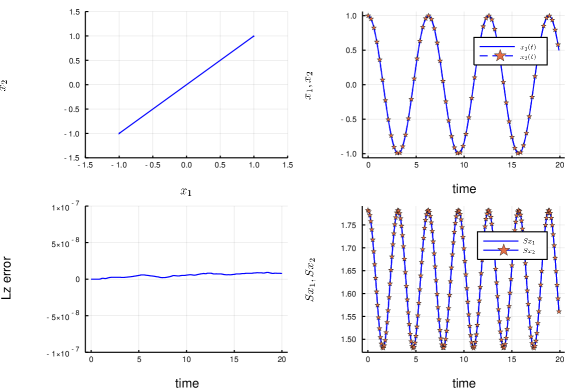
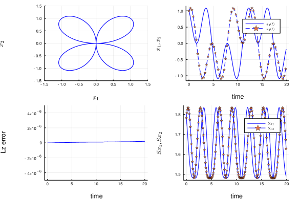
Figure 9: Time evolution of mass center, coordinates of mass center, error on angular momentum expectation, and condensate widths by ESQM when $\Omega=0$ (top four figures) and $\Omega=-0.5$ (bottom four figures).

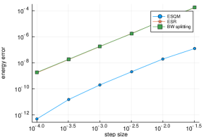
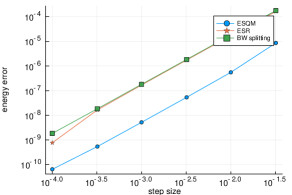
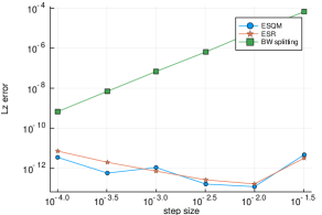
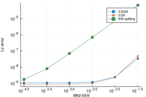
Figure 10: Energy error and angular momentum expectation error (semi-$\log_{10}$ scale) as a function of the step size for the three methods ESQM, ESR and BW at $t=1$ for $\Omega=-0.5$, when $\beta=5$, (a,c), $\beta=100$, (b,d).

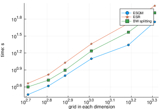
Figure 11: Comparisons of computational costs between ESQM, ESR, and BW by running $100$ steps for rotating GPE (LABEL:eq:gpe).

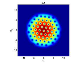
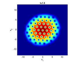
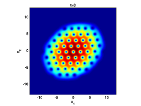
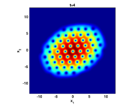
Figure 12: $\beta=1000,\Omega=0.9$. Time evolution of the solution of (LABEL:eq:gpe) by changing the potential initially.

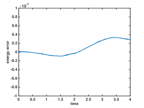
Figure 13: $\beta=1000,\Omega=0.9$. Time evolution of the energy of (LABEL:eq:gpe) by changing the potential initially.

5.4.2 3D Schrödinger equations

In this section, 3D Schrödinger equations are considered through two cases: $(i)$ a quadratic Schrödinger equation is constructed specifically such that the solution is periodic in time; $(ii)$ a magnetic Schrödinger equation with a non-quadratic potential (see [12]).

3D time-periodic quadratic linear Schrödinger equation
For (23), we consider $f=0$ and

$$B=\frac{\pi}{3}\begin{pmatrix}0&-1&1\\ 1&0&-1\\ -1&1&0\end{pmatrix}\quad\mbox{ and }\quad V({\bf x})=\frac{\pi^{2}}{9}\mskip 1.0mu\prescript{\smash{\mathrm{t}\mkern-3.0mu}}{}{\mathstrut{\bf x}}\begin{pmatrix}\lambda_{1}\\ &\lambda_{2}\\ &&\lambda_{3}\end{pmatrix}{\bf x},$$ (32)

where ${\bf x}=(x_{1},x_{2},x_{3})$ and $(\lambda_{1},\lambda_{2},\lambda_{3})$ are the roots of the polynomial $Q(X)=7200X^{3}-72196X^{2}+222088X-216341$, i.e.

$$\begin{pmatrix}\lambda_{1}\\ \lambda_{2}\\ \lambda_{3}\end{pmatrix}\simeq\begin{pmatrix}2.27017996551810\\ 2.53418020791380\\ 5.22286204879033\end{pmatrix}.$$ (33)

In this case, the period of this system is $T=360$ (see in Appendix 6.5 for the proof) and the initial condition is

$$\psi_{0}(x_{1},x_{2},x_{3})=\left(\frac{2}{\pi}\right)^{3}e^{-x_{1}^{2}}e^{-x_{2}^{2}}e^{-(x_{3}-1)^{2}}+i\left(\frac{2}{\pi}\right)^{3}e^{-x_{1}^{2}}e^{-(x_{2}+1)^{2}}e^{-(x_{3}-1)^{2}}.$$ (34)

The numerical parameters are chosen as: the spatial domain $[-8,8]^{3}$ is discretized by $N_{1}=N_{2}=N_{3}=96$ points, the time step is $\Delta t=0.2$, and the final time is $t=720$ which corresponds to two periods. We will consider two different methods:

• ESQM from (21) whose coefficients are listed in Appendix 6.3.1; the method is exact in time.

• Strang (see in Appendix 6.3.2); the method is second order accurate in time.

In Figures 14 and 15, the time evolution of $\psi(t,0,0,0)$ (real and imaginary parts) are presented by using ESQM and Strang respectively. We also plot the difference $\psi(t\in[T,2T],0,0,0)-\psi(t\in[0,T],0,0,0)$ (real and imaginary parts) which should be zero since the solution is time periodic of period $T=360$. We can see that with ESQM, the period is nicely preserved (up to $10^{-13}$) in spite of the fact that the time history of the solution is quite complicated. However, one can observe in Figure 15 that the conclusion is not the same for Strang: its error is too large to identify the period. In Figure 16, the time history of energy error is plotted for both ESQM and Strang methods. Clearly, Strang produces large errors whereas the error from ESQM is very small (only due to the space approximation). Concerning the computational cost, $6$ FFT (or inverse) are required for each time step for ESQM whereas Strang needs $15$ FFT (or inverse). Finally, some contour plots of the solution (at time $t=360$ and the third spatial direction $x_{3}$ is fixed to $0$) obtained by ESQM and Strang are presented at Figure 17. We expect $\psi(t=360,x_{1},x_{2},0)$ to be very close to the initial condition since the solution is $360$ periodic in time. Even if ESQM gives very accurate results, one can see in Figure 17 that the result obtained by Strang is rather different.

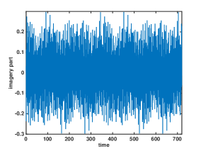
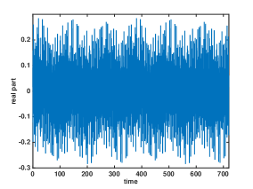
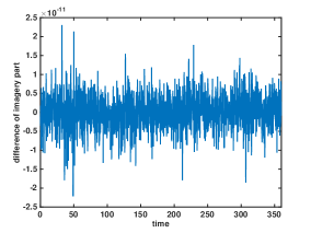
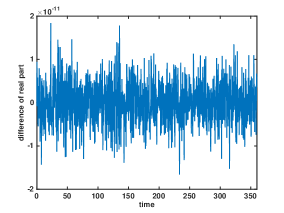
Figure 14: ESQM: (a) Time evolution of imaginary part of $\psi(t,0,0,0)$. (b) Time evolution of real part of $\psi(t,0,0,0)$. (c) The difference $\psi([T,2T],0,0,0)-\psi([0,T],0,0,0)$, $T=360$ (imaginary part). (d) The difference $\psi([T,2T],0,0,0)-\psi([0,T],0,0,0)$, $T=360$ (real part).

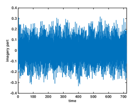
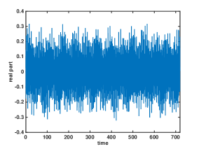
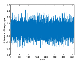
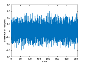
Figure 15: Strang: (a) Time evolution of imaginary part of $\psi(t,0,0,0)$. (b) Time evolution of real part of $\psi(t,0,0,0)$. (c) The difference $\psi([T,2T],0,0,0)-\psi([0,T],0,0,0)$, $T=360$ (imaginary part). (d) The difference $\psi([T,2T],0,0,0)-\psi([0,T],0,0,0)$, $T=360$ (real part).

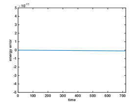
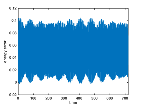
Figure 16: (a) Time evolution of the energy error by ESQM. (b) Time evolution of the energy error by Strang splitting.

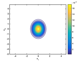
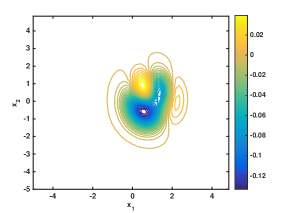
Figure 17: (a) Initial contour plot of the real part of $\psi(t=0,x_{1},x_{2},0)$; (b) contour plot of real part of $\psi(t=360,x_{1},x_{2},0)$ by ESQM; (c) contour plot of real part of $\psi(t=360,x_{1},x_{2},0)$ by Strang.

3D magnetic Schrödinger equation
To end this part, the following 3D magnetic Schrödinger equation is considered (see [12]),

$$i\partial_{t}\psi({\bf x},t)=-\frac{1}{2}\Delta\psi({\bf x},t)+i{\bf A}({\bf x})\cdot\nabla\psi({\bf x},t)+\frac{1}{2}|{\bf A}({\bf x})|^{2}\psi({\bf x},t)+V_{nq}({\bf x})\psi({\bf x},t),$$ (35)

where ${\bf A}({\bf x})={\bf x}\times{\bf B}$, ${\bf B}=\mskip 1.0mu\prescript{\smash{\mathrm{t}\mkern-3.0mu}}{}{\mathstrut(1,0.1,2)}$, ${\bf x}=(x_{1},x_{2},x_{3})$ and

$$V_{nq}({\bf x})=\alpha\left(20\cos(\frac{2\pi(x_{1}+5)}{10})+20\cos(\frac{2\pi(x_{2}+5)}{10})+20\cos(\frac{2\pi(x_{3}+5)}{10})+60\right),\alpha\in\mathbb{R}.$$ (36)

The initial condition is

$$\psi_{0}({\bf x})=\frac{2^{3/8}}{\pi^{3/2}}\exp\left(-\frac{\sqrt{2}}{2}((x_{1}-1)^{2}+x_{2}^{2}+x_{3}^{2})\right),$$

and the numerical parameters are: the spatial domain $[-5,5]^{3}$ is discretized by $N_{1}=N_{2}=N_{3}=64$ points and the final time is $t=1$. Here we consider three methods

• ESQM (see (25) with $f({\bf x},|\psi|^{2})=V_{nq}({\bf x})$ given by (36) and with (21)); this method is second order accurate in time.

• ESR (see Appendix 6.4); this method is second order accurate in time.

• Strang (see Appendix 6.4); this method is second order accurate in time.

The three methods are compared with different step sizes $\Delta t$ to solve the system (35). The energy errors of these three methods are presented in Figure 18, by studying the influence of the parameter $\alpha$ which measures the amplitude of the non-quadratic part in (35). By comparing the energy errors, we can see that the ESQM is the most accurate one, as it solves the linear quadratic part exactly. Moreover, when $\alpha$ is smaller, i.e., the non-quadratic term in system (35) becomes smaller, we can see that the advantage of ESQM is more obvious.

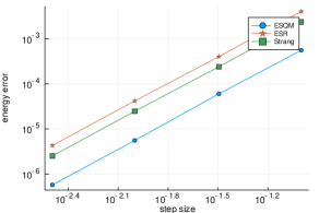
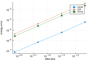
Figure 18: Plots of energy error with step size at $t=1$ with grids $N_{1}=N_{2}=N_{3}=64$. (a) $\alpha=0.1$, (b) $\alpha=0.01$.

6 Appendix

6.1 2D magnetic Schrödinger equation

$$i\epsilon\partial_{t}\psi({\bf x},t)=-\frac{\epsilon^{2}}{2}\Delta\psi({\bf x},t)+i\epsilon{\bf A}\cdot\nabla\psi({\bf x},t)+\frac{1}{2}{|\bf A|}^{2}\psi({\bf x},t),$$ (37)

where ${\bf x}=(x_{1},x_{2})\in\mathbb{R}^{2}$, ${\bf A}=\frac{1}{2}(A_{1},A_{2})$, $A_{1}=-x_{2}$, $A_{2}=x_{1}$. The above system can be split into three systems:

$$i\epsilon\partial_{t}\psi({\bf x},t)=-\frac{\epsilon^{2}}{2}\Delta\psi({\bf x},t),$$ (38)

$$\partial_{t}\psi({\bf x},t)={\bf A}\cdot\nabla\psi({\bf x},t),$$ (39)

$$i\epsilon\partial_{t}\psi({\bf x},t)=\frac{1}{2}{|\bf A|}^{2}\psi({\bf x},t),$$ (40)

The solutions of the above three subsystems can be obtained by operators $e^{it\frac{\epsilon}{2}\Delta}$, $e^{t\text{Rot}}$, and $e^{tV}$ respectively. Since the second is nothing but a 2D rotation, we call the associated solution $e^{t\text{Rot}}$. Then we have the following second order splitting method

$$\psi^{n+1}=e^{\frac{\Delta t}{2}V}e^{i\Delta t\frac{\epsilon}{4}\Delta}e^{\Delta t\text{Rot}}e^{i\Delta t\frac{\epsilon}{4}\Delta}e^{\frac{\Delta t}{2}V},$$ (41)

from which we derive two variants according to the treatment of $e^{\Delta t\text{Rot}}$. Indeed, ESR denotes the splitting method (41) when $e^{\Delta t\text{Rot}}$ is solved by exact splittings for transport equation in Proposition 1. Strang denotes (41) when $e^{\Delta t\text{Rot}}$ is approximated by Strang directional splitting.

6.2 2D rotating Gross-Pitaevskii equation

The rotating Gross-Pitaevskii equation (GPE) [6, 7] is

$${i}\partial_{t}\psi({\bf x},t)=-\frac{1}{2}\Delta\psi({\bf x},t)+V({\bf x})\psi({\bf x},t)+\beta|\psi|^{2}\psi({\bf x},t)-\Omega L_{x_{3}}\psi({\bf x},t),\ {\mathbf{x}}\in{\mathbb{R}}^{2},$$ (42)

where $\psi({\bf x},t)$ is the macroscopic wave function, ${\bf x}=(x_{1},x_{2})$, $L_{x_{3}}=-i(x_{1}\partial_{x_{2}}-x_{2}\partial_{x_{1}})$. Two operator splittings are presented to approximate (42).

6.2.1 ESR splitting

The above equation (42) can be split into three parts which can be solved exactly in time

$$i\frac{\partial\psi({\bf x},t)}{\partial t}=-\frac{1}{2}\Delta\psi({\bf x},t),$$

$$\frac{\partial\psi({\bf x},t)}{\partial t}=\Omega L_{x_{3}}\psi({\bf x},t),$$

$$i\frac{\partial\psi({\bf x},t)}{\partial t}=V({\bf x})\psi({\bf x},t)+\beta|\psi|^{2}\psi({\bf x},t).$$

The solutions of the above three subsystems can be obtained by operators $e^{-it\frac{1}{2}\Delta}$, $e^{t\text{Rot}}$, and $e^{t\text{VN}}$ respectively. Then we have the following second order method splitting method:

$$\psi^{n+1}({\mathbf{x}})=e^{\frac{\Delta t}{2}\text{VN}}e^{-i\Delta t\frac{1}{4}\Delta}e^{\Delta t\text{Rot}}e^{-i\Delta t\frac{1}{4}\Delta}e^{\frac{\Delta t}{2}\text{VN}}\psi^{n}({\mathbf{x}}),$$ (43)

from which we derive two variants according to the treatment of $e^{\Delta t\text{Rot}}$ (the part $e^{\frac{\Delta t}{2}\text{VN}}$ can be solved exactly). As for magnetic Schrödinger case, ESR denotes the splitting method (43) when $e^{\Delta t\text{Rot}}$ is solved by exact splittings for transport equation in Proposition 1.

6.2.2 BW method

Here we recall the splitting method introduced in [7] to approximate (42). We will call it BW in the sequel. BW splitting for rotating GPE (42) is based on the following two-steps splitting

$$i\partial_{t}\psi({\bf x},t)=-\frac{1}{2}\Delta\psi({\bf x},t)-\Omega L_{x_{3}}\psi({\bf x},t),$$ (44)

$$\partial_{t}\psi({\bf x},t)=V({\bf x})\psi({\bf x},t)+\beta|\psi({\bf x},t)|^{2}\psi({\bf x},t).$$ (45)

Then, the authors in [7] noticed that (44) can be split further as

$$i\partial_{t}\psi({\bf x},t)=-\frac{1}{2}\partial^{2}_{x_{1}}\psi({\bf x},t)-i\Omega x_{2}\partial_{x_{1}}\psi({\bf x},t),$$ (46)

$$i\partial_{t}\psi({\bf x},t)=-\frac{1}{2}\partial^{2}_{x_{2}}\psi({\bf x},t)+i\Omega x_{1}\partial_{x_{2}}\psi({\bf x},t).$$ (47)

The solutions of subsystems (45), (46) and (47) can be obtained by operators $e^{tN},e^{tX}$ and $e^{tY}$ respectively, the second order BW method is then derived from the following composition

$$\psi^{n}({\bf x}) =\left(e^{\Delta t/2\,Y}e^{\Delta t/2\,X}e^{\Delta t\,N}e^{\Delta t/2\,X}e^{\Delta t/2\,Y}\right)^{n}\psi_{0}({\bf x}),$$ (48)

$$=e^{\Delta t/2\,Y}(e^{\Delta t/2\,X}e^{\Delta t\,N}e^{\Delta t/2\,X}e^{\Delta t\,Y})^{n-1}e^{\Delta t/2\,X}e^{\Delta t\,N}e^{\Delta t/2\,X}e^{\Delta t/2\,Y}\psi_{0}({\bf x}).$$

Combined with Fourier pseudo-spectral method in space, we can see that in each time step, we need six calls to FFT.

6.3 3D time-periodic quadratic linear Schrödinger equation

For (23) with $f=0$ and $B$ and $V$ are specified in (32) and (33), we consider two numerical methods: ESQM and a standard Strang operator splitting.

6.3.1 Exact splitting

The coefficients for ESQM (21) are given by

$$A_{\Delta t}\simeq\begin{pmatrix}0.503369336514750&0.09260872887966&-0.086577853155386\\ 0.092608728879667&0.499175997238123&0.090475411725230\\ -0.086577853155386&0.090475411725230&0.482430618251455\end{pmatrix},$$

$$V_{\Delta t}^{(\ell)}\simeq\begin{pmatrix}1.838313777101704&0&0\\ 0&1.405233579215994&0\\ 0&0&2.416160688906186\end{pmatrix},$$

$$V_{\Delta t}^{(r)}\simeq\begin{pmatrix}0.765638127548775&0.097739062052903&-0.244124321719139\\ 0.097739062052903&1.408683914880933&0.141925135897144\\ -0.244124321719139&0.14192513589714&3.535113753227984\end{pmatrix},$$

$$L_{\Delta t}\simeq\begin{pmatrix}0&0&0\\ 0.957867410476376&0&0\\ -0.917880413070041&1.133563918623215&0\end{pmatrix},$$

$$U_{\Delta t}\simeq\begin{pmatrix}0&-1.132325985517193&0.915677911046419\\ 0&0&-0.957661219232001\\ 0&0&0\end{pmatrix}.$$

6.3.2 Strang method

Classically, we use the following operator splitting

$$i\frac{\partial\psi({\bf x},t)}{\partial t}=-\frac{1}{2}\Delta\psi({\bf x},t),$$

$$\frac{\partial\psi({\bf x},t)}{\partial t}=-({B}{\bf x})\cdot\nabla\psi({\bf x},t),$$

$$i\frac{\partial\psi({\bf x},t)}{\partial t}=V({\bf x})\psi({\bf x},t).$$

The solutions of the above three subsystems can be obtained by operators $e^{-it\frac{1}{2}\Delta}$, $e^{t\text{Rot}}$, and $e^{-it\text{V}}$ respectively so that we have the following second order splitting method

$$\psi^{n+1}({\mathbf{x}})=e^{-i\frac{\Delta t}{2}\text{V}}e^{-i\Delta t\frac{1}{4}\Delta}e^{\Delta t\text{Rot}}e^{-i\Delta t\frac{1}{4}\Delta}e^{-i\frac{\Delta t}{2}\text{V}}\psi^{n}({\mathbf{x}}).$$ (49)

Strang denotes (49) when $e^{\Delta t\text{Rot}}$ is also approximated by a Strang directional splitting.

6.4 3D magnetic Schrödinger equation

From (35), where ${\bf A}({\bf x})={\bf x}\times{\bf B}$, ${\bf B}=\mskip 1.0mu\prescript{\smash{\mathrm{t}\mkern-3.0mu}}{}{\mathstrut(1,0.1,2)}$ and $V$ given by (36), we can use the following operator splitting

$$i\frac{\partial\psi({\bf x},t)}{\partial t}=-\frac{1}{2}\Delta\psi({\bf x},t),$$

$$\frac{\partial\psi({\bf x},t)}{\partial t}={\mathbf{A}}({\bf x})\cdot\nabla\psi({\bf x},t),$$

$$i\frac{\partial\psi({\bf x},t)}{\partial t}=\frac{1}{2}|{\bf A}({\bf x})|^{2}\psi({\bf x},t)+V({\bf x})\psi({\bf x},t),$$

The solutions of the above three subsystems can be obtained by operators $e^{-it\frac{1}{2}\Delta}$, $e^{t\text{Rot}}$, and $e^{t\text{VA}}$ respectively and we can derive a second order splitting method:

$$\psi^{n+1}({\mathbf{x}})=e^{\frac{\Delta t}{2}\text{VA}}e^{-i\Delta t\frac{1}{4}\Delta}e^{\Delta t\text{Rot}}e^{-i\Delta t\frac{1}{4}\Delta}e^{\frac{\Delta t}{2}\text{VA}}\psi^{n}({\mathbf{x}}).$$ (50)

ESR denotes the splitting method (50) when $e^{\Delta t\text{Rot}}$ is solved by exact splittings for transport equation in Proposition 1. Strang denotes (50) when $e^{\Delta t\text{Rot}}$ is approximated by Strang directional splitting.

The coefficients when $\Delta t=0.1$ for ESQM (25) are as follows

$$A_{\Delta t}\simeq\begin{pmatrix}0.506160069704187&0.098840554692409&0.001683128724191\\ 0.098840554692409&0.508317718832811&0.050167780151672\\ 0.001683128724191&0.050167780151672&0.501715861437068\end{pmatrix},$$

$$V_{\Delta t}^{(\ell)}\simeq\begin{pmatrix}2.025343613765655&0&0\\ 0&0.508168767491105&0\\ 0&0&0.000099459606977\end{pmatrix},$$

$$V_{\Delta t}^{(r)}\simeq\begin{pmatrix}0.072891278447532&0.242556937819776&-1.026420948565178\\ 0.242556937819776&1.959142247295385&-0.046535665904951\\ -1.026420948565178&-0.046535665904951&0.508102737430800\end{pmatrix},$$

$$L_{\Delta t}\simeq\begin{pmatrix}0&0&0\\ 2.003434507092443&0&0\\ -0.099043028107977&1.016569585390557&0\end{pmatrix},$$

$$U_{\Delta t}\simeq\begin{pmatrix}0&-1.963756896350695&-0.099988990937417\\ 0&0&-1.006635420674690\\ 0&0&0\end{pmatrix}.$$

6.5 Proof of the period 360

Lemma 6.1.

The function $t\mapsto U_{t}=e^{it(\Delta/2-V(x))-tBx\cdot\nabla}$, where $V$ and $B$ are given by (32) satisfies

$$\forall t\in\mathbb{R},\ U_{t+180}=-U_{t}.$$

Proof.

Since $t\mapsto U_{t}$ is a group, we just have to prove that

$$U_{180}=-I_{L^{2}(\mathbb{R}^{3})}.$$

We recall that by construction, we have $U_{t}=e^{-tq_{\eqref{eq_QMS}}^{w}}$ where

$$q_{\eqref{eq_QMS}}^{w}=i\frac{|\boldsymbol{\xi}|^{2}}{2}+iB{\mathbf{x}}\cdot{\boldsymbol{\xi}}+iV({\mathbf{x}})$$

Step 1: To conjugate $q_{\eqref{eq_QMS}}^{w}$ to a sum of harmonic oscillators. We are going to prove that there exists $V\in\mathcal{U}(L^{2}(\mathbb{R}^{n}))$ such that

$$U_{t}=V\exp(-it\sum_{j=1}^{3}\omega_{j}(x_{j}^{2}-\partial_{x_{j}}^{2}))V^{*}$$ (51)

where $(\omega_{1},\omega_{2},\omega_{3})=\frac{\pi}{180}(20,75,132)$. Assuming first this decomposition, we deduce that

$$U_{180}=V\exp(-20i\pi(x_{1}^{2}-\partial_{x_{1}}^{2}))\exp(-75i\pi(x_{2}^{2}-\partial_{x_{2}}^{2}))\exp(-132i\pi(x_{3}^{2}-\partial_{x_{3}}^{2}))V^{*}.$$

But, in dimension $1$, the eigenvalues of the harmonic oscillator $x^{2}-\partial_{x}^{2}$ being the odd positive integers, we know that $\exp(i\pi(x^{2}-\partial_{x}^{2}))=-I_{L^{2}(\mathbb{R}^{3})}$. Thus, we deduce that

$$U_{180}=VI_{L^{2}(\mathbb{R}^{3})}(-I_{L^{2}(\mathbb{R}^{3})})I_{L^{2}(\mathbb{R}^{3})}V^{*}=-I_{L^{2}(\mathbb{R}^{3})}.$$

In order to prove (51) we are going to apply the following theorem due to Hörmander.

Theorem 6.1 (Hörmander, Theorem 21.5.3 in [22]).

Let $Q\in S_{2n}^{++}(\mathbb{R})$ be a real symmetric positive matrix of size $2n$. There exists a real symplectic matrix $P\in\mathrm{Sp}_{2n}(\mathbb{R})$ of size $2n$ such that and some positive numbers $\omega_{1},\dots,\omega_{n}$ such that

$$\mskip 1.0mu\prescript{\smash{\mathrm{t}\mkern-3.0mu}}{}{\mathstrut P}QP=D(\omega)$$

where $D(\omega)=\mathrm{diag}(\omega_{1},\dots,\omega_{n},\omega_{1},\dots,\omega_{n})$ is the diagonal matrix such that, for $j=1,\dots,n$, $D(\omega)_{j,j}=D(\omega)_{j+n,j+n}=\omega_{j}$ .

Indeed, here, it can be checked that $Q_{\eqref{eq_QMS}}$ (the matrix of $q_{\eqref{eq_QMS}}$) is a symmetric positive matrix (computing, for example, an approximation of its eigenvalues). Thus, applying Theorem 6.1, we get a symplectic matrix $P$ and some positive numbers $\omega_{1}<\omega_{2}<\omega_{3}$ such that

$$\mskip 1.0mu\prescript{\smash{\mathrm{t}\mkern-3.0mu}}{}{\mathstrut P}Q_{\eqref{eq_QMS}}P=D(\omega).$$ (52)

Consequently, since $P$ is symplectic, we have

$$\exp(2tJQ_{\eqref{eq_QMS}})=P\exp(2tJD(\omega))P^{-1},$$

where $J$ is the symplectic matrix of $\mathbb{R}^{2n}$. Now, applying the monoid morphism (Theorem 3.1 in [8]) introduced also by Hörmander in [21], we get a function $t\mapsto\sigma_{t}\in\{\pm 1\}$ such that

$$\forall t\in\mathbb{R},\ U_{t}=e^{-itq_{\eqref{eq_QMS}}^{w}}=\sigma_{t}V\exp(-it\sum_{j=1}^{3}\omega_{j}(x_{j}^{2}-\partial_{x_{j}}^{2}))V^{*}$$

where $\pm V$ is the Fourier Integral Operator associated with $P$. Note that $V$ is unitary. Furthermore, by a straighforward argument of continuity we deduce that $\sigma_{t}=1$ for all $t\in\mathbb{R}$. Thus, to conclude, we just have to prove that $(\omega_{1},\omega_{2},\omega_{3})=\frac{\pi}{180}(20,75,132)$.

Step 2: To determine $\omega$. First, we observe that the matrices $JQ_{\eqref{eq_QMS}}$ and $JD(\omega)$ are similar. Indeed, since $P\in\mathrm{Sp}_{6}(\mathbb{R})$, we have $\mskip 1.0mu\prescript{\smash{\mathrm{t}\mkern-3.0mu}}{}{\mathstrut P}\in\mathrm{Sp}_{6}(\mathbb{R})$ and applying (52) we deduce that

$$JD(\omega)=J\mskip 1.0mu\prescript{\smash{\mathrm{t}\mkern-3.0mu}}{}{\mathstrut P}Q_{\eqref{eq_QMS}}P=(P^{-1}J\mskip 1.0mu\prescript{\smash{\mathrm{t}\mkern-3.0mu}}{}{\mathstrut P}^{-1})\mskip 1.0mu\prescript{\smash{\mathrm{t}\mkern-3.0mu}}{}{\mathstrut P}Q_{\eqref{eq_QMS}}P=P^{-1}JQ_{\eqref{eq_QMS}}P.$$

A fortiori, $JQ_{\eqref{eq_QMS}}$ and $JD(\omega)$ have the same eigenvalues. Thus, the eigenvalues of $JQ_{\eqref{eq_QMS}}$ are

$$\sigma(JQ_{\eqref{eq_QMS}})=\sigma(JD(\omega))=\{i\omega_{1},-i\omega_{1},i\omega_{2},-i\omega_{2},i\omega_{3},-i\omega_{3}\}.$$ (53)

Consequently, to determine $\omega$ we just have to determine the roots of the characteristic polynomial of $JQ_{\eqref{eq_QMS}}$, denoted $\chi_{\eqref{eq_QMS}}$. By a straightforward calculation, we observe that

$$\left(\frac{3}{\pi}\right)^{6}\chi_{\eqref{eq_QMS}}(\frac{\pi X}{3})=X^{6}+\frac{\lambda_{1}+\lambda_{2}+\lambda_{3}+3}{2}X^{4}+\frac{\lambda_{1}\lambda_{2}+\lambda_{1}\lambda_{3}+\lambda_{2}\lambda_{3}+9/4}{4}X^{2}\\ -3\frac{\lambda_{1}+\lambda_{2}+\lambda_{3}}{32}+\frac{\lambda_{1}\lambda_{2}+\lambda_{1}\lambda_{3}+\lambda_{2}\lambda_{3}}{8}-\frac{\lambda_{1}\lambda_{2}\lambda_{3}}{8}.$$

But, by construction $\lambda_{1}<\lambda_{2}<\lambda_{3}$ are the roots of the polynomial

$$7200X^{3}-72196X^{2}+222088X-216341.$$

Thus, $\lambda_{1}+\lambda_{2}+\lambda_{3}$, $\lambda_{1}\lambda_{2}+\lambda_{1}\lambda_{3}+\lambda_{2}\lambda_{3}$ and $\lambda_{1}\lambda_{2}\lambda_{3}$ are some explicit rational numbers and we deduce that

$$\left(\frac{3}{\pi}\right)^{6}\chi_{\eqref{eq_QMS}}(\frac{\pi X}{3})=X^{6}+\frac{407}{120}X^{4}+\frac{123}{80}X^{2}-\frac{7}{384}.$$

Finally, we verify by an explicit computation that

$$\chi_{\eqref{eq_QMS}}(i\frac{\pi}{9})=\chi_{\eqref{eq_QMS}}(i\frac{5\pi}{12})=\chi_{\eqref{eq_QMS}}(i\frac{11\pi}{15})=0.$$

So, we deduce of (53) that $(\omega_{1},\omega_{2},\omega_{3})=\frac{\pi}{180}(20,75,132)$. ∎

References

- [1] P. Alphonse, J. Bernier, Polar decomposition of semigroups generated by non-selfadjoint quadratic differential operators and regularizing effects, hal-02280971, 2019.
- [2] J. Ameres, Splitting methods for Fourier spectral discretizations of the strongly magnetized Vlasov-Poisson and the Vlasov-Maxwell system, arXiv preprint arXiv:1907.05319, 2019.
- [3] X. Antoine, W. Bao, C. Besse, Computational methods for the dynamics of the nonlinear Schrödinger/Gross-Pitaevskii equations, Computer Physics Communications, 2013, 184 (12), pp. 2621-2633?
- [4] X. Antoine, R. Duboscq, GPELab, a Matlab toolbox to solve Gross-Pitaevskii equations I: Computation of stationary solutions, Computer Physics Communications, 2014, 185 (11), pp. 2969-2991.
- [5] X. Antoine, R. Duboscq, Gpelab, a matlab toolbox to solve Gross-Pitaevskii equations II: Dynamics and stochastic simulations, Computer Physics Communications, 2015, 193, pp. 95-117.
- [6] W. Bao, Q. Du, Y. Zhang, Dynamics of rotating Bose-Einstein condensates and its efficient and accurate numerical computation, SIAM Journal on Applied Mathematics, 2006, 66 (3), pp. 758-786.
- [7] W. Bao, H. Wang, An efficient and spectrally accurate numerical method for computing dynamics of rotating Bose-Einstein condensates, Journal of Computational Physics, 2006, 217 (2), pp. 612-626.
- [8] J. Bernier, Exact splitting methods for semigroups generated by inhomogeneous quadratic differential operators, preprint.
- [9] J. Bernier, F. Casas, N. Crouseilles, Splitting methods for rotations: application to Vlasov equations, accepted in SIAM J. of Scientific Comput.
- [10] C. Besse, G. Dujardin, I. Lacroix-Violet, High order exponential integrators for nonlinear Schrödinger equations with application to rotating Bose-Einstein condensates, SIAM Journal on Numerical Analysis, 2017, 55 (3), pp. 1387-1411.
- [11] N. Besse, M. Mehrenberger, Convergence of classes of high-order semi-Lagrangian schemes for the Vlasov-Poisson system, Mathematics of computation, 2008, 77 (261), pp. 93-123.
- [12] M. Caliari, A. Ostermann, C. Piazzola, A splitting approach for the magnetic Schrödinger equation, Journal of Computational and Applied Mathematics, 2017, 316, pp. 74-85.
- [13] B. Chen, A. Kaufman, 3D volume rotation using shear transformations, Graphical Models, 2000, 62 (4), pp. 308-322.
- [14] O. Coulaud, E. Sonnendrücker, E. Dillon, P. Bertrand, J. Plasma Physics, 1999, 61, pp. 435-448.
- [15] G. Dujardin, F. Hérau, P. Lafitte, Coercivity, hypocoercivity, exponential time decay and simulations for discrete Fokker-Planck equations, arXiv preprint arXiv:1802.02173, 2018.
- [16] E. Hairer, C. Lubich, G. Wanner, Geometric numerical integration: Structure-Preserving Algorithms for Ordinary Differential Equations, Springer Series in Computational Mathematics, 2006.
- [17] F. Hérau, J. Sjöstrand, M. Hitrik, Tunnel effect for the Kramers-Fokker-Planck type operators: return to equilibrium and applications, Int. Math. Res. Not., 2008, 57, p. 48.
- [18] F. Hérau, J. Sjöstrand, M. Hitrik, Tunnel effect for the Kramers-Fokker-Planck type operators, Ann. Henri Poincaré, 2008, 9, pp. 209-274.
- [19] F. Hérau, L. Thomann, On global existence and trend to the equilibrium for the Vlasov-Poisson-Fokker-Planck system with exterior confining potential, J. Funct. Anal, 2016, 271, pp. 1301-1340.
- [20] M. Hochbruck, A. Ostermann, Exponential integrators, Acta Numerica, 2010, 19, pp. 209-286.
- [21] L. Hörmander, Symplectic classification of quadratic forms, and general Mehler formulas, Math. Z., (1995), 219, pp. 413-449.
- [22] L. Hörmander, The analysis of linear partial differential operators. III, Classics in Mathematics, Springer, Berlin, 2007. Pseudo-differential operators, https://doi.org/10.1007/978-3-540-49938-1
- [23] S. Jin, Z. Zhou, A semi-Lagrangian time splitting method for the Schrödinger equation with vector potentials, Communications in Information and Systems, 2013, 13 (3), pp. 247-289.
- [24] Y. Li, Y. He, Y. Sun, et al., Solving the Vlasov-Maxwell equations using Hamiltonian splitting, Journal of Computational Physics, 2019, 396, pp. 381-399
- [25] R.I. McLachlan, G.R. Quispel, Splitting methods, Acta Numerica, 2002, 11, pp. 341-434.
- [26] J.E. Marsden, T.S.Ratiu, Introduction to mechanics and symmetry: a basic exposition of classical mechanical systems, Springer Science & Business Media, 2013.
- [27] N. Raymond, Bound States of the Magnetic Schrödinger Operator, EMS Tracts in Mathematics, 2017.
- [28] J.S. Welling, W.F. Eddy, T.K. Young, Rotation of 3D volumes by Fourier-interpolated shears, Graphical Models, 2006, 68 (4), pp. 356-370.
- [29] R. Zeng, Y. Zhang, Efficiently computing vortex lattices in rapid rotating Bose-Einstein condensates, Computer Physics Communications, 2009, 180 (6), pp. 854-860.