CASE: Context-Aware Semantic Expansion

Abstract

In this paper, we define and study a new task called Context-Aware Semantic Expansion (CASE). Given a seed term in a sentential context, we aim to suggest other terms that well fit the context as the seed. CASE has many interesting applications such as query suggestion, computer-assisted writing, and word sense disambiguation, to name a few. Previous explorations, if any, only involve some similar tasks, and all require human annotations for evaluation. In this study, we demonstrate that annotations for this task can be harvested at scale from existing corpora, in a fully automatic manner. On a dataset of 1.8 million sentences thus derived, we propose a network architecture that encodes the context and seed term separately before suggesting alternative terms. The context encoder in this architecture can be easily extended by incorporating seed-aware attention. Our experiments demonstrate that competitive results are achieved with appropriate choices of context encoder and attention scoring function.

Introduction

Have you ever googled “Lionel Messi championships”, browsed the results, and wanted more soccer stars with comparable championships? Have you ever wanted to know types of nutrients rich in barley grass, but were only able to remember amino acid? In this paper, we study context-aware semantic expansion (or CASE for short). In CASE, user provides a seed term wrapped in a sentential context as in Figure 1. The system returns a list of expansion terms, each of which is a valid substitute for the seed, i.e., the substitution is supported by some sentence in a (testing) corpus. This task is not easy due to the large number of potential expansions, as well as the necessity of modeling their interactions with both the context and the seed. Despite the challenge, the task is of practical importance and benefits many applications. We list a few examples here.

Query suggestion (?). In the aforementioned query “Lionel Messi championships”, keywords “Lionel Messi” can be a seed term to expand, and a CASE system may suggest related entities, e.g., “Christiano Ronaldo”, as expansion terms. Those terms may be used to suggest queries like “Christiano Ronaldo championships”.

Computer-assisted writing (?). For casual or academic writing, exemplifications often help to explain and convince. It is desirable to suggest contextually appropriate alternative words when an author can think of only one.

Other NLP tasks. CASE can potentially enhance natural language processing (NLP) tasks. For example, in word sense disambiguation (?), an ambiguous word like “apple” can be first expanded w.r.t. its context. The suggested context-aware terms (e.g., fruits or companies) provide cues for the disambiguation task.

[leftmargin=0.8cm] Seed in context: “Young barley grass is high in amino acid.”
Expansion terms: vitamin, antioxidant, enzyme, mineral, chlorophyll, …

Figure 1: A seed term “amino acid” in context. Here, “fat” is an invalid substitute. It is irrelevant to barley grass and tends not to be supported by general corpora.

Comparison with Related Tasks

Despite its significance, explorations on CASE remain limited. Lexical substitution (?) is the most similar task to CASE. Given a word in a sentential context, e.g., “the bright girl is reading a book”, lexical substitution predicts synonyms fitting the context, e.g., “wise” or “clever” rather than “shining”. The synonym candidates generally come from high-quality but relatively small dictionaries like WordNet (?). Compared with lexical substitution, candidate expansion terms of CASE, e.g., entity names, are not required to be aliases of the seeds but could be far more in number and less organized.

Besides lexical substitution, another task similar to CASE is set expansion (?; ?; ?; ?; ?; ?). It is to expand a few seeds (e.g., amino acid and vitamin) to more terms in the same semantic class (i.e., nutrition). However, set expansion does not involve possible textual contexts with the seeds. This may cause “fat” to appear in the results of Figure 1, which is irrelevant to barley grass.

While the above two tasks differ considerably from CASE by task definition, we further note that their model tuning and evaluation require manual annotations, which are hard to collect at scale. Fortunately, CASE benefits from large-scale natural annotations, as described below.

Dataset and Formal Task Definition

A first step toward CASE with today’s deep learning machinery is to accumulate large-scale annotations. For this task, an ideal piece of annotation would be different terms appearing separately in identical contexts. While this form of annotations is hard to obtain manually and rare in natural corpora, we note that people often list examples, which effectively serve as natural annotations.

In a general corpus, lists of examples usually follow Hearst patterns (?; ?), e.g., “h such as t₁, t₂, …”, “t₁, t₂, …, and other h”, etc. Here h denotes a hypernym, and {t_i} are hyponyms. We note that, in the context, if all hyponyms other than one is removed, the sentence is still “correct” in the sense of the corpus.

By post-processing a web-scale corpus (detailed in experiments), we derive a collection of 1.8 million naturally annotated sentences. All of them are of the form $\langle C,T\rangle$ as below.

Context $C$: “Young barley grass is high in      and other phyto-nutrients.”

Terms $T$: {vitamin, antioxidant, enzyme, mineral, amino acid, chlorophyll}

Here $C$ is the sentential context with a placeholder “    ”. $T=\{t_{i}\}$ are hyponyms appearing at the placeholder in Hearst patterns. The CASE task is to use a seed term $s\in T$ and the context $C$ to recover the remaining terms $T\setminus\{s\}$.

Taking advantage of the large dataset derived, we propose a neural network architecture with attention mechanism (?) to learn supervised expansion models. Readers may notice that, due to the use of Hearst patterns, the context $C$ above has an additional hypernym “phyto-nutrient” compared with Figure 1. In experiments, in addition to comparisons among solutions, we will also study the impact of this gap.

To summarize, our contributions are:

• We define and study a novel task, i.e., CASE, which supports many interesting and important applications.

• We identify an easy yet effective method to collect natural annotations.

• We propose a neural network architecture for CASE, and further enhance it with the attention mechanism. On millions of naturally annotated sentences, we experimentally verify the superiority of our model.

Model Overview

Given the inherent variability of natural language and the sufficient annotations, we tackle CASE by a supervised neural-network-based approach.

Our network to model $P(.|s,C)$ is shown in Figure 2. The network consists of three parts: a context encoder, a seed encoder, and a prediction layer. Given a seed $s$ in a context $C$, the network encodes them into two vectors $\mathbf{v}_{s}$ and $\mathbf{v}_{C}$ with the seed and context encoders, respectively. The two vectors are then concatenated as input to the prediction layer to predict potential expansion terms.

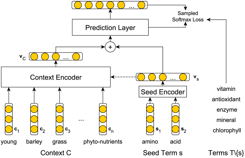
Figure 2: The network architecture of CASE.

On training sentences $\mathcal{T}$, we aim to optimize:

$$\max\sum_{\langle C,T\rangle\in\mathcal{T}}\sum_{s\in T}\log P(T\setminus\{s\}|s,C)$$ (1)

Note that, a sentence $\langle C,T\rangle$ is regarded as $|T|$ training samples. Each sample treats one term as the seed, and predicts the other terms within the context. In the remainder of this section, we briefly describe each of the three components.

Encoding Sentential Contexts

Given one or two seed terms, the traditional set expansion task simply finds other terms in the same semantic class. However, the sentential context $C$ may contain additional descriptions or restrictions, thus narrowing down the scope of the listed terms. Therefore, it is vital to appropriately model $C$ to capture its underlying information in CASE.

In Figure 2, we employ the context encoder component to encode a variable-length context $C$ into a fixed-length vector $\mathbf{v}_{C}$. There are various off-the-shelf neural models to encode sentences or sentential contexts. On the one hand, by treating $C$ as a bag or a sequence of words, conventional sentence encoders may be applied, e.g., Neural Bag-of-Words (NBoW) (?), RNN (?), and CNN (?). On the other hand, there are also techniques that explicitly model placeholders, e.g., CNN with positional features (?) and context2vec (?). In this paper, we mainly investigate NBoW-based and RNN-based encoders. We also involve other encoders for comparison, e.g., CNN-based and placeholder-aware encoders.

Neural Bag-of-Words Encoder. Given words $\{c_{i}\}_{i=1}^{n}$ in a context $C$, an NBoW encoder looks up their vectors $\mathbf{c}_{i}\in\mathbb{R}^{d}$ in an embedding matrix, and average the vectors as $\mathbf{v}_{C}=\frac{1}{n}\sum_{i=1}^{n}\mathbf{c}_{i}$. The word embedding matrix is initialized with embeddings pre-trained on the original sentences in training set, and is updated during training. Due to its simplicity, NBoW is efficient to train. However, it ignores the order of context words.

RNN- and CNN-Based Encoders. To study the impact of word order on context encoding, we consider RNN-based encoders as alternatives to NBoW. RNNs take a sequence of context word vectors $(\mathbf{c}_{1},\mathbf{c}_{2},\dots,\mathbf{c}_{n})$, and iteratively encodes information before each position $i$ as a sequence of hidden vectors $(\mathbf{h}_{1},\mathbf{h}_{2},\dots,\mathbf{h}_{n})$, $\mathbf{h}_{i}\in\mathbb{R}^{d}$. Following ? (?), we take the last hidden vector $\mathbf{h}_{n}$ as the context vector $\mathbf{v}_{C}$:

$$\mathbf{h}_{i} =\text{RNN}(\mathbf{c}_{i},\mathbf{h}_{i-1})\text{,}\quad i=1\dots n\text{,}$$ (2)

$$\mathbf{v}_{C} =\mathbf{h}_{n}\text{.}$$ (3)

Besides the vanilla version of RNN, other RNN variations like LSTM (?), GRU (?), and bi-directional LSTM (BiLSTM) (?) have proven effective in various NLP tasks. In our experiments, we compare all these RNN variations.

Other than the NBoW- and RNN-based encoders described above, CNNs (?) have also been used as sentence encoders (?; ?; ?). Specifically, we perform the convolution operation on the input vector sequence $(\mathbf{c}_{1},\mathbf{c}_{2},\dots,\mathbf{c}_{n})$, and apply max-pooling to get the context representation $\mathbf{v}_{C}$.

Position-Aware Encoders. All above encoders ignore the the position of the placeholder, i.e., where the seed term appears. For CASE, one may hypothesize that words at different distances to the placeholder contributes differently to $\mathbf{v}_{C}$. ? (?) propose CNN with positional features (CNN+PF) as a counterpart for CNN. Each context word vector $\mathbf{c}_{i}$ fed into CNN is concatenated with a position vector $\mathbf{p}_{i}$ that models its distance to the placeholder. The positional vectors are treated as parameters and updated during training. In context2vec (?), two LSTMs are used to encode the left and right contexts of placeholders, respectively. The output are concatenated as the final context representation $\mathbf{v}_{C}$. We implement and compare it with BiLSTM as a counterpart.

Encoding the Seed Term

Due to its short length, we simply adopt the same NBoW to encode seed term, for it is less prone to overfitting (?). Given words $\{s_{i}\}_{i=1}^{m}$ of a seed term $s$, we obtain $\mathbf{v}_{s}$ by $\mathbf{v}_{s}=\frac{1}{m}\sum_{i=1}^{m}\mathbf{s}_{i}$. Because of their different role, seed word embeddings $\mathbf{s}_{i}\in\mathbb{R}^{d}$ are from another embedding matrix, but are initialized and updated in the same manner with context word embeddings.

Predicting Expansion Terms

After encoding the seed and the context into $\mathbf{v}_{s}$ and $\mathbf{v}_{C}$, respectively, we feed their concatenation $\mathbf{x}=\mathbf{v}_{s}\oplus\mathbf{v}_{C}$ to the prediction layer for expansion terms. We treat the prediction as a classification problem, and each candidate term as a classification label. Given a sufficiently large $\mathcal{T}$, we consider all terms appearing in Hearst pattern lists in $\mathcal{T}$ as candidates, and constitute the label set $L$ by pooling them, i.e., $L=\cup_{\langle C,T\rangle\in\mathcal{T}}T$. The prediction layer is then instantiated by a fully connected layer (with bias) followed by a softmax layer over $L$. The probability of a term $t$ is then

$$P(t|s,C)=\frac{\exp(\mathbf{w}_{t}^{\top}\mathbf{x}+b_{t})}{\sum_{t^{\prime}\in L}\exp(\mathbf{w}_{t^{\prime}}^{\top}\mathbf{x}+b_{t^{\prime}})}\quad\text{.}\\$$ (4)

Here $\{\textbf{w}_{t},b_{t}\}_{t\in L}$ are weight and bias parameters of the fully connected layer.

Note that we simultaneously predict multiple terms, i.e., $T\setminus\{s\}$, so the classification is essentially multi-labeled. Moreover, the softmax layer introduces summed exponentials on the denominator of $P(t|s,C)$. This makes training inefficient on a large $L$ (over 180k on our dataset). To relieve both issues, we use a multi-label implementation of sampled softmax loss (?). That is, a much smaller candidate set from $L$ is sampled to approximate gradients related to $L$.

Incorporating Attention on Contexts

So far, we have detailed various encoders for context $C$. They all essentially aggregate the information in every word with or without position information in $C$. Given potentially long input $C$ and the fixed output dimension, it is vital for encoders to capture the most useful information into $\mathbf{v}_{C}$.

Recent studies (?; ?; ?; ?) suggest that attention-based encoders can focus on more important parts of sentences, thus achieving better representations. In this section, we explore approaches to incorporate attention into the context encoders. Based on whether they exploit information in the seed term, we categorize them as seed-oblivious or seed-aware.

Seed-Oblivious Attention

By seed-oblivious attention, we aim to model the importance of different words or positions in a sentential context. Following conventional approaches (?), we use a feed-forward network to estimate the importance of each word or position. For the NBoW encoder, the importance score of word $i$ is defined by

$$f(i) =\mathbf{w}_{a}^{\top}\tanh(\mathbf{W}_{a}\mathbf{c}_{i})\text{.}$$ (5)

Here $\mathbf{w}_{a}\in\mathbb{R}^{d^{\prime}}$ and $\mathbf{W}_{a}\in\mathbb{R}^{d^{\prime}\times d}$ are parameters of the feed-forward network. The score $f(i)$ is then fed through a softmax layer and used as weights to combine the word vectors $\mathbf{c}_{i}$:

$$\alpha_{i} =\frac{\exp(f(i))}{\sum_{i^{\prime}}\exp(f(i^{\prime}))}\text{,}$$ (6)

$$\mathbf{v}_{C} =\sum_{i=1}^{n}\alpha_{i}\mathbf{c}_{i}\text{.}$$ (7)

For RNN, attention is applied in a similar manner, except that $\mathbf{c}_{i}$ is substituted by hidden vector $\mathbf{h}_{i}$.

Seed-Aware Attention

So far, we have discussed various context encoders and an attention-based improvement. For them, the seed does not contribute to context encoding. However, a seed like “amino acid” may conversely indicate informative words or parts in the context, e.g., “barley” and “grass”, to further narrow down the semantic scope of expansion. Following this observation, we propose involving the seed vector $\mathbf{v}_{s}$ to compute a seed-aware importance score $f(s,i)$ instead of $f(i)$. Inspired by ? (?), we consider the following instantiations of seed-aware attention.

dot In this variant, we estimate the word importance with the inner product of the seed vector $\mathbf{v}_{s}$ and each word vector $\mathbf{c}_{i}$. Formally, the score is

$$f(s,i)=\mathbf{v}_{s}^{\top}\mathbf{c}_{i}\text{.}$$ (8)

concat Instead of directly taking the inner product of $\mathbf{v}_{s}$ and $\mathbf{c}_{i}$, this variant feeds their concatenation through a feed-forward network:

$$f(s,i)=\mathbf{w}_{a}^{\top}\tanh(\mathbf{W}_{a}[\mathbf{v}_{s};\mathbf{c}_{i}])\text{.}$$ (9)

Here $\mathbf{w}_{a}\in\mathbb{R}^{d^{\prime}}$ and $\mathbf{W}_{a}\in\mathbb{R}^{d^{\prime}\times 2d}$ are parameters of the feed-forward network. By involving additional parameters $\mathbf{w}_{a}$ and $\mathbf{W}_{a}$, we expect the concat variant to be more capable than dot.

trans-dot In dot, we multiply the seed and word vectors $\mathbf{v}_{s}$ and $\mathbf{c}_{i}$. Note that the context word vectors $\mathbf{c}_{i}$ need to both interact with the seed vector $\mathbf{v}_{s}$ and constitute the context representation $\mathbf{v}_{C}$. To distinguish between the two potentially different roles, we additionally consider the following trans-dot scoring function:

$$f(s,i)=\mathbf{v}_{s}^{\top}\tanh(\mathbf{W}_{a}\mathbf{c}_{i})\text{.}$$ (10)

Here, we use a fully connected layer with parameters $\mathbf{W}_{a}\in\mathbb{R}^{d\times d}$ to transform $\mathbf{c}_{i}$ before taking a dot product with $\mathbf{v}_{s}$. Compared with dot, the trans-dot scoring function only introduce a medium-sized parameter space, which is smaller than that of concat.

In order to apply seed-aware attention to our network structure, we use the respective scoring functions $f(s,i)$ to replace $f(i)$ in Eq. 6. The resulted attention weights $\alpha_{s,i}$ are fed to Eq. 7, and make the context vector $\mathbf{v}_{C}$ seed-aware.

Experimental Settings

Dataset Processing

Item	Count
Number of sentences	1,847,717
Number of training sentences $|\mathcal{T}|$	1,478,173
Number of testing sentences	369,544
Average number of context words $|C|$	31.39
Average number of hyponym terms $|T|$	3.46
Number of unique terms	182,167
Number of unique terms on training set $|L|$	180,684
Vocabulary size of all contexts	941,603
Vocabulary size of all training contexts	119,270
(discarding words with freq $<5$)

Table 1: Summary of the derived dataset.

We earlier briefed that CASE exploits sentences with Hearst patterns for training and evaluation. For this reason, large-scale natural annotations can be easily obtained without manual effort.

Specifically, we employ an existing web-scale dataset, WebIsA (?), to derive large-scale annotated sentences. This dataset has 400 million hypernymy relations, extracted from 2.1 billion web pages. For each hyponym-hypernym pair, the dataset provides IDs of source sentences and matched patterns where the pair occurs. For example, a sentence “Young barley grass is high in vitamin, antioxidant, enzyme, mineral, amino acid, chlorophyll and other phyto-nutrients.” leaves its ID and pattern “…and other …” in the lists of hypernymy pairs “vitamin $\rightarrow$ phyto-nutrient”, “antioxidant $\rightarrow$ phyto-nutrient”, etc. Precisions of all patterns are also summarized as global information. We use the information to decompose the sentence, obtaining the example in the Dataset and Formal Task Definition section. Specifically, we follow the below steps.

1. We convert all words to lowercase and lemmatize them.

2. We then filter the dataset with the pattern precision information, due to the noisy web pages and the error-prone hypernymy extraction procedure. That is, we identify and keep high-quality sentences where a hypernym is extracted with at least three hyponyms by a pattern with precision $\geq 0.5$.

3. We regard hyponym terms appearing in at least ten high-quality sentences as high-quality terms. We select high-quality sentences with at least three high-quality terms in the final dataset.

Finally, our dataset contains 1,847,717 naturally labeled sentences, involving over 180k hyponym terms. From them, we sample 20% of sentences to form the test set, and use the remainder for training. Table 1 summarizes our dataset.

Baseline Approaches

Since no previous study addresses the exact CASE task, we evaluate our models against the solutions proposed for the most similar task, i.e., lexical substitution. Specifically, we compare with ? (?)’s unsupervised method and one of its variants. We also evaluate a supervised method by ? (?).

Lexical Substitution (LS). Word embedding models such as ? (?) compute two types of word vectors, i.e., IN and OUT. ? (?)’s analysis suggests that the IN-IN similarity favors synonyms or words with similar functions, while the IN-OUT similarity characterizes word compatibility or co-occurrence. By promoting terms $t$ having the same meaning with the seed $s$ and good compatibility with the context $C$, they score a term $t$ by

$$\textsc{LS}=\lambda_{1}cos(\mathbf{s}^{I},\mathbf{t}^{I})+\frac{1-\lambda_{1}}{|C|}\sum_{c\in C}cos(\mathbf{c}^{I},\mathbf{t}^{O})$$ (11)

Here the superscripts $I$ and $O$ stands for IN and OUT, respectively. We train word vectors on all sentences in $\mathcal{T}$, and use averaged vectors to represent multi-word terms. We follow the original paper and set $\lambda_{1}=0.5$.

LS with Term Co-occurrence (LSCo). Considering that expansion terms are not simply synonyms of seeds, and tend to co-occur with seeds (in Hearst patterns), we also study a modified version of Eq. 11:

$$\textsc{LSCo}=\lambda_{2}\textsc{LS}+(1-\lambda_{2})cos(\mathbf{s}^{I},\mathbf{t}^{O})$$ (12)

We tune $\lambda_{2}$ and adopt the best-effort results.

Probability In Context (PIC) (?). Different from the second term of Eq. 11, PIC models the context compatibility by introducing a parameterized linear transformation on $\mathbf{c}^{I}$. Therefore, it needs data to train the additional parameters and is inherently supervised.

Parameters and Evaluation Metrics

We trim or pad all contexts to length 100, and treat words occurring less than 5 times as OOVs. Word vectors are pre-trained with cbow (?). Their dimensions $d$ as well as encoded contexts’ and seeds’ are set to 100. The intermediate dimension $d^{\prime}$ of attention-related network is set to 10. Each batch is of size 128 with 1,000 negative samples to compose the sampled candidates. We iterate for 10 epoches with the Adam optimizer. All other hyper-parameters are found to work well by default and not tuned.

Figure 3: Tuning $\lambda_{2}$ in the LSCo baseline.

Model	Recall	MAP	MRR	nDCG
LS (?)	2.84	1.80	1.79	1.66
LSCo ($\lambda_{2}=0.1$)	3.54	2.65	2.69	2.23
PIC (?)	19.62	17.78	18.84	14.71
CASE (ours, with NBoW)	23.42	21.30	22.71	17.80

Table 2: Comparison with LS baselines (top-10 results).

For all approaches, we uniformly rank all $t\in L$ according to the corresponding probability. We concentrate on top-10 results. Note that, due to the nature of natural language, ground-truth term lists may not be exhaustive. This is an intrinsic limitation of the original dataset, and our processed dataset is probably the best we can access. To this end, we use Recall as the main metric and do not involve Precision. We also report MAP, MRR, and nDCG for reference.

Experimental Results

In this section, we aim to experimentally answer the following questions: 1) Are lexical substitution solutions applicable to CASE? 2) Do contexts have impact on semantic expansion? 3) Is seed-aware attention superior as expected? 4) Do additional hypernyms make the experiments biased?

Comparison with LS Baselines

When introducing ? (?)’s lexical substitution baseline, we mention that expansion terms should co-occur with, rather than be synonyms of, the seed term. In Figure 3, we compare the Recall@10 scores of baselines LS and LSCo, w.r.t. different $\lambda_{2}$. Note that LSCo degenerates to LS when $\lambda_{2}=1$, so their lines overlap at this point. The figure demonstrates that, when $\lambda_{2}<1$, the LSCo baseline outperforms LS, and achieves optimum when $\lambda_{2}=0.1$.

In Table 2, we report the top-10 metrics of all three lexical substitution baselines, as well as those of our approach with the preliminary NBoW encoder. By additionally advocating co-occurrence between $s$ and $t$, LSCo outperforms LS on all metrics. However, it is remarkably inferior due to its unsupervised nature.

By parameterizing the context compatibility in LS, PIC achieves reasonably better results. However, PIC only models the similarity of seed and expansion terms through non-parameterized IN-IN similarity like the first term in Eq. 11. This may be inadequate, with reasons similar to the inferiority of LS to LSCo. In our solution, the embedding-initialized parameters allow our seed encoder and prediction layer to capture type-based similarity beyond IN-IN and IN-OUT through training. With the simplest NBoW encoder, the joint training of the two components helps our approach outperform PIC by a large margin.

Context Encoder	Recall	MAP	MRR	nDCG
No Encoder	15.81	14.02	14.85	11.62
RNN-Based
RNN-vanilla	17.51	16.17	17.08	13.26
GRU	18.99	17.28	18.31	14.24
LSTM	19.02	17.40	18.43	14.31
BiLSTM	14.59	13.45	14.22	10.96
CNN	20.97	19.40	20.61	15.94
Placeholder-Aware
CNN+PF	20.88	19.04	20.20	15.70
context2vec	20.21	18.53	19.66	15.29
NBoW	23.42	21.30	22.71	17.80

Table 3: Performance of context encoders (top-10 results).

Model	Recall			MAP			MRR			nDCG
	@5	@10	@20	@5	@10	@20	@5	@10	@20	@5	@10	@20
LSTM	13.08	19.02	26.19	16.80	17.40	17.14	17.15	18.43	19.13	11.88	14.31	16.73
+attn	13.73	19.85	27.15	17.72	18.29	17.96	18.11	19.41	20.11	12.55	15.04	17.51
NBoW	16.32	23.42	31.64	20.78	21.30	20.79	21.29	22.71	23.45	14.91	17.80	20.58
+attn	16.69	23.88	32.24	21.36	21.87	21.30	21.89	23.32	24.06	15.29	18.22	21.06
+dot	15.54	22.13	29.89	20.12	20.60	20.12	20.61	21.95	22.66	14.36	17.03	19.66
+concat	16.85	24.12	32.53	21.57	22.04	21.47	22.10	23.54	24.28	15.46	18.41	21.27
+trans-dot	17.20	24.51	33.01	21.97	22.41	21.80	22.53	23.96	24.70	15.80	18.77	21.65

Table 4: Performance of different scoring functions in attention. trans-dot is significantly better at $p<0.01$.

Comparison of Context Encoders

The Introduction section mentioned that set expansion is similar to CASE without context. We find that one seed is usually sufficient to retrieve terms of the same type. The result thus heavily depend on the context to pick the right terms out of many others with the same type. Table 3 reflects this by the inferior results of the “No Encoder” setting, where contexts are removed in both training and testing.

Although contexts are important, complex encoders do not necessarily lead to better results. In Table 3, encoders at lower semantic levels, i.e., NBoW at the word level and CNN at the phrase level, are the most effective. Among them, the simpler NBoW achieves better scores. Moreover, RNN-based ones are not very competitive, with the best LSTM variation poorer than CNN. This may be due to that RNNs are only effective where predictions are sensitive to word orders, e.g., in POS tagging and dependency parsing. Finally, being placeholder-aware, the context2vec encoder performs better than its LSTM counterpart. However, CNN with positional embedding, the stronger placeholder-aware encoder, is inferior to its CNN counterpart. This indicates that CASE is inherently different from tasks like relation classification and aspect/targeted sentiment analysis, which rely on relative position between the placeholder and some key words.

With Hypernym		Without Hypernym
NBoW	+trans-dot	NBoW	+trans-dot
protein	mineral	protein	mineral
sugar	sugar	calcium	etc
vitamin	protein	salt	sugar
mineral	vitamin	sugar	vitamin
carbohydrate	b vitamin	vitamin	protein
herb	enzyme	enzyme	herb
enzyme	amino acid	herb	carbohydrate
fat	herb	potassium	salt
fiber	antioxidant	mineral	fat
salt	salt	etc	vitamin c

Table 5: Case study on attention and hypernyms.

Based on the above observations, we confirm that contexts have major impacts on CASE and deserve appropriate modeling. However, complex encoders are inferior because CASE is insensitive to either word orders or seed term positions. Modeling these signals leads to more unnecessary parameters to learn and brings in noises.

Effectiveness of the Attention Mechanism

In previous sections, we proposed two types of scoring functions to incorporate the attention mechanism in the context encoder. In Table 4, we denote the vanilla seed-oblivious attention by attn, and the three seed-aware functions by their names, respectively. Due to the relatively small margin between the scores of different functions, we report the metrics for top-5 and 20 results in addition to top-10. Although seed-aware attention is applicable to LSTM, we do not include the results since they do not outperform the corresponding combinations of NBoW. The limited improvement may be due to the low potential of the base LSTM encoder.

Table 4 shows that seed-oblivious attention can improve both LSTM and NBoW. Although seed-aware, the dot scoring function turns out to adversely affect the quality of expansion terms. We speculate that the two different roles of context word vectors $\mathbf{c}$ render the simple dot function insufficient to characterize its interactions with $\mathbf{v}_{s}$. The concat function, on the other hand, partially demonstrates superiority of seed-aware attention with limited improvement over attn. By slightly modifying dot with even fewer additional parameters than concat, trans-dot outperforms all competitors. Further paired t-tests show that the superiority of trans-dot (as well as the most competitive runs in Tables 2 and 3) to all competitors is significant at $p<0.01$. We attribute the statistical significance to the huge size of our testing set, i.e., 369,544 sentences.

To illustrate the impact of trans-dot, we show expansion terms of “amino acid” for the example in the Dataset and Formal Task Definition section, in the first two columns of Table 5. Observe that trans-dot-based attention helps promote the ground truth terms (in bold) in the ranking. It also removes nutrition “fat” from the top results, which is irrelevant to barley grass.

Impacts of Hypernyms

Model (w/o Hypernym)	Recall	MAP	MRR	nDCG
NBoW	22.64	20.68	22.03	17.22
+trans-dot	23.41	21.52	22.98	17.94

Table 6: Scores after removing hypernyms (top-10 results).

The contexts from WebIsA always contain hypernyms, e.g., “phyto-nutrients” in the example of the Dataset and Formal Task Definition section. However, practical scenarios may involve sentences without hypernyms as in Figure 1. To study the potential impact, we remove all hypernyms in contexts, retrain and test NBoW with or without trans-dot. The last two columns in Table 5 show the results of our running example without the suffix “and other phyto-nutrients”. It is observed that removing hypernyms causes some non-nutrient or noisy terms (e.g., “salt” and “etc”) to rise. Table 6 reports the overall scores for top-10 results. Compared with the corresponding results in Table 4, all scores slightly decrease by around one point. This comparison suggests that, trained with sufficient term co-occurrences, our model is able to find terms of the same types, without the help of hypernyms in most cases. To conclude, the hypernym bias introduced by the data harvesting approach has very small impacts on the practical use of our solution.

Related Work

Lexical Substitution This task has been investigated for over a decade (?). It differs from CASE in that the substitutes are required to preserve the same meaning with the original word. Previous solutions follow two stages, i.e., candidate generation and candidate ranking. Synonym candidates are generally generated from external dictionaries or by pooling the testing data. The ranking stage then boils down to estimating the compatibility between candidates and the context.

? (?) rely on n-grams to model candidates’ compatibility. ? (?) argues that syntactic relations in contexts are crucial, e.g., “a horse draws something” and “someone draws a horse”. In ? (?), word vectors (?) are applied to score candidates’ similarity with the original word and their context compatibility. Their method is nearly state-of-the-art, yet remains relatively simple. Besides unsupervised approaches, supervised methods (?; ?; ?) prove superior at the cost of requiring more annotations. We have experimentally compared with representative ones from both categories.

Set Expansion This task aims to expand a couple of seeds to more terms in the underlying semantic class. Most existing approaches involve bootstrapping on a large corpus of web pages (?; ?; ?; ?) or free text (?; ?; ?; ?). HTML-tag-based or lexical patterns covering a few seeds are extracted, which are then applied to the same corpus for new terms. The process is iterated until certain stopping criterion is met.

Both this task and ours face the challenge of ambiguous terms, e.g., “apple”. With multiple seeds, set expansion may rely on the other seeds, e.g., “samsung” or “orange”, for disambiguation. However, since CASE accepts only one seed as input, it is essential to model the additional context to make up for the scarce information. To this end, we resort to neural networks, where many off-the-shelf context modeling architectures are available.

Multi-Sense or Contextualized Word Representation This technique deals with sense-mixing in traditional word representation. Traditional word representations assign a single vector to each word. They mix different senses of polysemous words, and block downstream tasks from exploiting the sense information. ? (?) cluster the contexts of polysemous words and represent senses by the cluster centroids. By sequentially carrying out context clustering, sense labeling, and representation learning, ? (?) obtain low-dimensional sense embeddings. Non-parametric (?) and probabilistic models with fewer parameters (?) are proposed later to accelerate training.

In multi-sense embedding, polysemous words get static embeddings for coarse-grained senses. Some recent efforts explore dynamic embeddings that vary with the context. ? (?) use context-aware substitutions of target words to obtain contextualized embeddings. ? (?) employ multi-layered bi-directional language models on words in contexts. Embeddings are obtained by aggregating different hidden layers with task-specific weights. CASE separately models contexts and seed terms, because the model needs to generalize to unseen multi-word seeds. For more studies, we refer readers to a survey (?).

Conclusion

We define and address context-aware semantic expansion. To the best of our knowledge, this is the first study on this task. To facilitate training and evaluation without human annotations, we derive a large dataset with about 1.8 million naturally annotated sentences from WebIsA. We propose a network structure, and study different alternatives of the context encoder. Experiments show that solutions for lexical substitution are not competitive on CASE. Comparisons on various context encoders indicate that, the simplest NBoW encoder achieves surprisingly good performance. Based on NBoW, seed-aware attention, which models the interaction between seed and context words, further improves the performance. The trans-dot scoring function finally shows its capability to focus on indicative words, and outperforms other seed-oblivious or -aware competitors. In further analysis, we also confirm small impacts of a bias introduced when harvesting our data.

References

- Bahdanau, Cho, and Bengio 2014 Bahdanau, D.; Cho, K.; and Bengio, Y. 2014. Neural machine translation by jointly learning to align and translate. arXiv preprint arXiv:1409.0473.
- Camacho-Collados and Pilehvar 2018 Camacho-Collados, J., and Pilehvar, T. 2018. From word to sense embeddings: A survey on vector representations of meaning. arXiv preprint arXiv:1805.04032.
- Chen, Cafarella, and Jagadish 2016 Chen, Z.; Cafarella, M.; and Jagadish, H. 2016. Long-tail vocabulary dictionary extraction from the web. In WSDM.
- Chung et al. 2014 Chung, J.; Gulcehre, C.; Cho, K.; and Bengio, Y. 2014. Empirical evaluation of gated recurrent neural networks on sequence modeling. arXiv preprint arXiv:1412.3555.
- Erk and Padó 2008 Erk, K., and Padó, S. 2008. A structured vector space model for word meaning in context. In ENNLP.
- Fellbaum 1998 Fellbaum, C. 1998. WordNet. Wiley Online Library.
- Giuliano, Gliozzo, and Strapparava 2007 Giuliano, C.; Gliozzo, A.; and Strapparava, C. 2007. Fbk-irst: Lexical substitution task exploiting domain and syntagmatic coherence. In SemEval.
- Graves and Schmidhuber 2005 Graves, A., and Schmidhuber, J. 2005. Framewise phoneme classification with bidirectional lstm and other neural network architectures. Neural Networks.
- He and Xin 2011 He, Y., and Xin, D. 2011. Seisa: set expansion by iterative similarity aggregation. In WWW.
- Hearst 1992 Hearst, M. A. 1992. Automatic acquisition of hyponyms from large text corpora. In COLING.
- Hochreiter and Schmidhuber 1997 Hochreiter, S., and Schmidhuber, J. 1997. Long short-term memory. Neural computation.
- Hu et al. 2014 Hu, B.; Lu, Z.; Li, H.; and Chen, Q. 2014. Convolutional neural network architectures for matching natural language sentences. In NIPS.
- Huang et al. 2012 Huang, E. H.; Socher, R.; Manning, C. D.; and Ng, A. Y. 2012. Improving word representations via global context and multiple word prototypes. In ACL.
- Jean et al. 2015 Jean, S.; Cho, K.; Memisevic, R.; and Bengio, Y. 2015. On using very large target vocabulary for neural machine translation. In ACL-IJCNLP.
- Kalchbrenner, Grefenstette, and Blunsom 2014 Kalchbrenner, N.; Grefenstette, E.; and Blunsom, P. 2014. A convolutional neural network for modelling sentences. In ACL.
- Kim 2014 Kim, Y. 2014. Convolutional neural networks for sentence classification. In EMNLP.
- LeCun et al. 1989 LeCun, Y.; Boser, B.; Denker, J. S.; Henderson, D.; Howard, R. E.; Hubbard, W.; and Jackel, L. D. 1989. Backpropagation applied to handwritten zip code recognition. Neural computation.
- Liu et al. 2011 Liu, C.-L.; Lee, C.-H.; Yu, S.-H.; and Chen, C.-W. 2011. Computer assisted writing system. ESA.
- Luong, Pham, and Manning 2015 Luong, T.; Pham, H.; and Manning, C. D. 2015. Effective approaches to attention-based neural machine translation. In EMNLP.
- McCarthy and Navigli 2007 McCarthy, D., and Navigli, R. 2007. Semeval-2007 task 10: English lexical substitution task. In SemEval.
- Melamud et al. 2015 Melamud, O.; Levy, O.; Dagan, I.; and Ramat-Gan, I. 2015. A simple word embedding model for lexical substitution. In NAACL-HLT.
- Melamud, Dagan, and Goldberger 2015 Melamud, O.; Dagan, I.; and Goldberger, J. 2015. Modeling word meaning in context with substitute vectors. In NAACL-HLT.
- Melamud, Goldberger, and Dagan 2016 Melamud, O.; Goldberger, J.; and Dagan, I. 2016. context2vec: Learning generic context embedding with bidirectional lstm. In CoNLL.
- Mikolov et al. 2013 Mikolov, T.; Sutskever, I.; Chen, K.; Corrado, G. S.; and Dean, J. 2013. Distributed representations of words and phrases and their compositionality. In NIPS.
- Navigli 2009 Navigli, R. 2009. Word sense disambiguation: A survey. ACM Computing Surveys.
- Neelakantan et al. 2014 Neelakantan, A.; Shankar, J.; Passos, A.; and McCallum, A. 2014. Efficient non-parametric estimation of multiple embeddings per word in vector space. In EMNLP.
- Pearlmutter 1989 Pearlmutter, B. A. 1989. Learning state space trajectories in recurrent neural networks. Neural Computation.
- Peters et al. 2018 Peters, M.; Neumann, M.; Iyyer, M.; Gardner, M.; Clark, C.; Lee, K.; and Zettlemoyer, L. 2018. Deep contextualized word representations. In NAACL-HLT.
- Reisinger and Mooney 2010 Reisinger, J., and Mooney, R. J. 2010. Multi-prototype vector-space models of word meaning. In NAACL-HLT.
- Roller and Erk 2016 Roller, S., and Erk, K. 2016. Pic a different word: A simple model for lexical substitution in context. In NAACL-HLT.
- Seitner et al. 2016 Seitner, J.; Bizer, C.; Eckert, K.; Faralli, S.; Meusel, R.; Paulheim, H.; and Ponzetto, S. P. 2016. A large database of hypernymy relations extracted from the web. In LREC.
- Shen et al. 2017 Shen, J.; Wu, Z.; Lei, D.; Shang, J.; Ren, X.; and Han, J. 2017. Setexpan: Corpus-based set expansion via context feature selection and rank ensemble. In ECML-PKDD.
- Shi et al. 2010 Shi, S.; Zhang, H.; Yuan, X.; and Wen, J.-R. 2010. Corpus-based semantic class mining: distributional vs. pattern-based approaches. In COLING.
- Shi et al. 2014 Shi, B.; Zhang, Z.; Sun, L.; and Han, X. 2014. A probabilistic co-bootstrapping method for entity set expansion. In COLING.
- Shimaoka et al. 2017 Shimaoka, S.; Stenetorp, P.; Inui, K.; and Riedel, S. 2017. Neural architectures for fine-grained entity type classification. In EACL.
- Snow, Jurafsky, and Ng 2005 Snow, R.; Jurafsky, D.; and Ng, A. Y. 2005. Learning syntactic patterns for automatic hypernym discovery. In NIPS.
- Szarvas, Biemann, and Gurevych 2013 Szarvas, G.; Biemann, C.; and Gurevych, I. 2013. Supervised all-words lexical substitution using delexicalized features. In NAACL-HLT.
- Szarvas, Busa-Fekete, and Hüllermeier 2013 Szarvas, G.; Busa-Fekete, R.; and Hüllermeier, E. 2013. Learning to rank lexical substitutions. In EMNLP.
- Thelen and Riloff 2002 Thelen, M., and Riloff, E. 2002. A bootstrapping method for learning semantic lexicons using extraction pattern contexts. In Proceedings of the ACL-02 conference on Empirical methods in natural language processing-Volume 10, 214–221. Association for Computational Linguistics.
- Tian et al. 2014 Tian, F.; Dai, H.; Bian, J.; Gao, B.; Zhang, R.; Chen, E.; and Liu, T.-Y. 2014. A probabilistic model for learning multi-prototype word embeddings. In COLING.
- Tong and Dean 2008 Tong, S., and Dean, J. 2008. System and methods for automatically creating lists. US Patent 7,350,187.
- Wang and Cohen 2007 Wang, R. C., and Cohen, W. W. 2007. Language-independent set expansion of named entities using the web. In ICDM.
- Wang et al. 2016 Wang, Y.; Huang, M.; Zhao, L.; and Zhu, X. 2016. Attention-based lstm for aspect-level sentiment classification. In EMNLP.
- Wen, Nie, and Zhang 2001 Wen, J.-R.; Nie, J.-Y.; and Zhang, H.-J. 2001. Clustering user queries of a search engine. In WWW.
- Zeng et al. 2014 Zeng, D.; Liu, K.; Lai, S.; Zhou, G.; and Zhao, J. 2014. Relation classification via convolutional deep neural network. In COLING.