LinearPartition: Linear-Time Approximation of RNA Folding Partition Function and Base Pairing Probabilities

Abstract

RNA secondary structure prediction is widely used to understand RNA function. Recently, there has been a shift away from the classical minimum free energy (MFE) methods to partition function-based methods that account for folding ensembles and can therefore estimate structure and base pair probabilities. However, the classical partition function algorithm scales cubically with sequence length, and is therefore a slow calculation for long sequences. This slowness is even more severe than cubic-time MFE-based methods due to a larger constant factor in runtime. Inspired by the success of our recently proposed LinearFold algorithm that predicts the approximate MFE structure in linear time, we design a similar linear-time heuristic algorithm, LinearPartition, to approximate the partition function and base pairing probabilities, which is shown to be orders of magnitude faster than Vienna RNAfold and CONTRAfold (e.g., 2.5 days vs. 1.3 minutes on a sequence with length 32,753 nt). More interestingly, the resulting base pairing probabilities are even better correlated with the ground truth structures. LinearPartition also leads to a small accuracy improvement when used for downstream structure prediction on families with the longest length sequences (16S and 23S rRNA), as well as a substantial improvement on long-distance base pairs (500+ nt apart).
See http://github.com/LinearFold/LinearPartition for code and http://linearfold.org/partition for server.

-2pt

1 Introduction

RNAs are involved in multiple processes, such as catalyzing reactions or guiding RNA modifications ^{1, 2, 3}, and their functionalities are highly related to structures. However, structure determination techniques, such as X-ray crystallography ⁴, Nuclear Magnetic Resonance (NMR) ⁵, and cryo-electron microscopy ⁶, though reliable and accurate, are extremely slow and costly. Therefore, fast and accurate computational prediction of RNA structure is useful and desired. Considering full RNA structure prediction is challenging ⁷, many studies focus on predicting secondary structure, the set of canonical base pairs in the structure (A-U, G-C, G-U base pairs) ⁸, as it is well-defined, and provides detailed information to help understand the structure-function relationship, and is a basis to predict full tertiary structure ^{9, 10}.

A

B

C

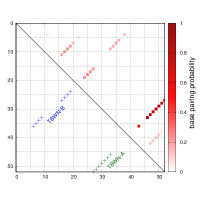
D
 span minimum free energy partition-function bottom-up, exact $\infty$ Zuker¹¹ $O(n^{3})$ McCaskill¹² $O(n^{3})$ local folding $L$ Localfold¹³ $O(nL^{2})$ RNAplfold¹⁴ $O(nL^{2})$ Rfold¹⁵ left-to-right, exact $\infty$ LinearFold ¹⁶ $O(n^{3})$ LinearPartition $O(n^{3})$  + beam pruning $O(nb\log b)$ $O(nb^{2})$

Figure 1: An RNA can fold into multiple structures at equilibrium. A–B: Two secondary structures of Tebowned RNA: TBWN-A and TBWN-B ¹⁷. C: upper triangle shows the estimated base pairing probability matrix for this RNA using Vienna RNAfold, where darker red squares represent higher probility base pairs; the lower triangle shows the two different structures; D: Comparison between classical, local, and left-to-right algorithms for MFE and partition function calculation. LinearFold and LinearPartition enjoy linear runtime because of a left-to-right order that enables heuristic beam pruning, and both become exact $O(n^{3})$ algorithms without pruning. “Span” denotes the maximum pair distance allowed ($\infty$ means no limit); it is a small constant in local methods (e.g., default $L$=70 nt in RNAplfold).

RNA secondary structure prediction is NP-complete ¹⁸, but nested (i.e., pseudoknot-free) secondary structures can be predicted with cubic-time dynamic programming algorithms. Commonly, the minimum free energy (MFE) structure is predicted ^{19, 11}. At equilibrium, the MFE structure is the most populated structure, but it is a simplification because multiple conformations exist as an equilibrium ensemble for one RNA sequence ²⁰. For example, many mRNAs in vivo form a dynamic equilibrium and fold into a population of structures ^{21, 22, 23, 24}; Figure 1A–B shows the example of Tebowned RNA which folds into more than one structure at equilibrium. In this case, the prediction of one single structure, such as the MFE structure, is not expressive enough to capture multiple states of RNA sequences at equilibrium.

Alternatively, we can compute the partition function, which is the sum of the equilibrium constants for all possible secondary structures, and is the normalization term for calculating the probability of a secondary structure in the Boltzmann ensemble. The partition function calculation can also be used to calculate base pairing probabilities of each nucleotide $i$ paired with each of possible nucleotides $j$ ^{12, 20}. In Figure 1C, the upper triangle presents the base pairing probability matrix of Tebowned RNA using Vienna RNAfold, showing that base pairs in TBWN-A have higher probabilities (in darker red) than base pairs in TBWN-B (in lighter red). This is consistent with the experimental result, i.e., TBWN-A is the majority structure that accounts for $56\pm 16\%$ of the ensemble, while TBWN-B takes up $27\pm 12\%$ ¹⁷.

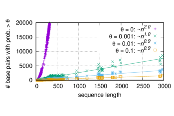
Figure 2: Although the total number of possible base pairings scales $O(n^{2})$ with the sequence length $n$ (using the probability matrix from Vienna RNAfold as an example), with any reasonable threshold $\theta$, the number of surviving pairings (in colors for different $\theta$) grows linearly, suggesting our approximation, only computing $O(n)$ pairings, is reasonable.

In addition to model multiple states at equilibrium, base pairing probabilities are used for downstream prediction methods, such as maximum expected accuracy (MEA) ^{25, 26}, to assemble a structure with improved accuracy compared with the MFE structure ²⁷. Other downstream prediction methods, such as ProbKnot ²⁸, ThreshKnot ²⁹, DotKnot ³⁰ and IPknot ³¹, use base pairing probabilities to predict pseudoknotted structures with heuristics, which is beyond the scope of standard cubic-time algorithms. Additionally, the partition function is the basis of stochastic sampling, in which structures are sampled with their probability of occurring in the Boltzmann ensemble ^{32, 33}.

Therefore, there has been a shift from the classical MFE-based methods to partition function-based ones. These latter methods, as well as the prediction engines based on them, such as partition function-mode of RNAstructure ³⁴, Vienna RNAfold ³⁵, and CONTRAfold ²⁶, are all based on the seminal algorithm that McCaskill pioneered ¹². It employs a dynamic program to capture all possible (exponentially many) nested structures, but its $O(n^{3})$ runtime still scales poorly for longer sequences. This slowness is even more severe than the $O(n^{3})$-time MFE-based ones due to a much larger constant factor. For instance, for H. pylori 23S rRNA (sequence length 2,968 nt), Vienna RNAfold’s computation of the partition function and base pairing probabilities is 9$\times$ slower than MFE (71 vs. 8 secs), and CONTRAfold is even 20$\times$ slower (120 vs. 6 secs). The slowness prevents their applications to longer sequences.

To address this $O(n^{3})$-time bottleneck, we present LinearPartition, which is inspired by our recently proposed LinearFold algorithm ¹⁶ that approximates the MFE structure in linear time. Using the same idea, LinearPartition can approximate the partition function and base pairing probability matrix in linear time. Like LinearFold, LinearPartition scans the RNA sequence from 5’-to-3’ using a left-to-right dynamic program that runs in $O(n^{3})$ time, but unlike the classical bottom-up McCaskill algorithm ¹² with the same speed, our left-to-right scanning makes it possible to apply the beam pruning heuristic ³⁶ to achieve linear runtime in practice; see Fig 1D. Although the search is approximate, the well-designed heuristic ensures the surviving structures capture the bulk of the free energy of the ensemble. It is important to note that, unlike local folding methods in Fig. 1D, our algorithm does not impose any limit on the base-pairing distance; in other words, it is a global partition function algorithm.

More interestingly, as Figure 2 shows, even with the $O(n^{3})$-time McCaskill algorithm, the resulting number of base pairings with reasonable probabilities (e.g., >0.001) grows only linearly with the sequence length. This suggests that our algorithm, which only computes $O(n)$ pairings by design, is a reasonable approximation.

LinearPartition is 2,771$\times$ faster than CONTRAfold for the longest sequence (32,753 nt) that CONTRAfold can run in the dataset (2.5 days vs. 1.3 min.). Interestingly, LinearPartition is orders of magnitude faster without sacrificing accuracy. In fact, the resulting base pairing probabilities are even better correlated with ground truth structures, and when applied to downstream structure prediction tasks, they lead to a small accuracy improvement on longer families (small and large subunit rRNA), as well as a substantial accuracy improvement on long-distance base pairs (500+ nt apart).

Although both LinearPartition and LinearFold use linear-time beam search, the success of the former is arguably more surprising, since rather than finding one single optimal structure, LinearPartition needs to sum up exponentially many structures that capture the bulk part of the ensemble free energy. LinearPartition also results in more accurate downstream structure predictions than LinearFold.

2 The LinearPartition Algorithm

We denote $\mathbf{x}\!=\!x_{1}...x_{n}$ as the input RNA sequence of length $n$, and $\mathcal{Y(\mathbf{x})}$ as the set of all possible secondary structures of $\mathbf{x}$. The partition function is:

$$Q(\mathbf{x})=\sum_{\mathbf{y}\in\mathcal{Y(\mathbf{x})}}e^{-\frac{\Delta G^{\circ}({\mathbf{y}})}{RT}}$$

where $\Delta G^{\circ}({\mathbf{y}})$ is the conformational Gibbs free energy change of structure $\mathbf{y}$, $R$ is the universal gas constant and $T$ is the thermodynamic temperature. $\Delta G^{\circ}({\mathbf{y}})$ is calculated using loop-based Turner free-energy model ^{37, 38}, but for presentation reasons, we use a revised Nussinov-Jacobson energy model, i.e., a free energy change of $\delta(\mathbf{x},j)$ for unpaired base at position $j$ and a free energy change of $\xi(\mathbf{x},i,j)$ for base pair of $(i,j)$. For example, we can assign $\delta(\mathbf{x},j)\!=\!1$ kcal/mol and $\xi(\mathbf{x},i,j)\!=\!-3$ kcal/mol for CG pairs and $-2$ kcal/mol for AU and GU pairs. Thus, $\Delta G^{\circ}({\mathbf{y}})$ can be decomposed as:

$$\Delta G^{\circ}({\mathbf{y}})=\sum_{j\in\text{unpaired}(\mathbf{y})}\delta(\mathbf{x},j)\ +\sum_{(i,j)\in\text{pairs}(\mathbf{y})}\xi(\mathbf{x},i,j)$$

where ${\textrm{unpaired}}(\mathbf{y})$ is the set of unpaired bases in $\mathbf{y}$, and ${\textrm{paired}}(\mathbf{y})$ is the set of base pairs in $\mathbf{y}$. The partition function now decomposes as:

$$Q(\mathbf{x})=\sum_{\mathbf{y}\in\mathcal{Y(\mathbf{x})}}(\prod_{j\in\text{unpaired}(\mathbf{y})}e^{-\frac{\delta(\mathbf{x},j)}{RT}}\prod_{(i,j)\in\text{pairs}(\mathbf{y})}e^{-\frac{\xi(\mathbf{x},i,j)}{RT}})$$

We first define span $[i,j]$ to be the subsequence $x_{i}...x_{j}$ (thus $[1,n]$ denotes the whole sequence $\mathbf{x}$, and $[j,j\!-\!1]$ denotes the empty span between $x_{j-1}$ and $x_{j}$ for any $j$ in $1..n$). We then define a state to be a span associated with its partition function:

$$[i,j]:Q_{{{i}},{{j}}}$$

where

$\displaystyle Q_{{{i}},{{j}}}=\sum_{\mathbf{y}\in\mathcal{Y}(x_{i}...x_{j})}e^{-\frac{\Delta G^{\circ}(\mathbf{y})}{RT}}$

encompasses all possible substructures for span $[i,j]$, which can be visualized as ​$\ \ Q_{{{i}},{{j}}}\ \$​ $i$ $j$ .

1:function LinearPartition($\mathbf{x},b$) $\triangleright$ $b$ is the beam size

2:  $n\leftarrow$ length of $\mathbf{x}$

3:  $Q\leftarrow$ hash() $\triangleright$ hash table: from span $[i,j]$ to $Q_{{{i}},{{j}}}$

4:  $Q_{{{j}},{{j-1}}}\leftarrow 1$ for all $j$ in $1...n$ $\triangleright$ base cases

5:  for $j=1...n$ do

6:   for each $i$ such that $[i,\,j-1]$ in $Q$ do $\triangleright$ $O(b)$ iterations

7:    $Q_{{{i}},{{j}}}\mathrel{+}=Q_{{{i}},{{j-1}}}\cdot e^{-\frac{\delta(\mathbf{x},j)}{RT}}$ $\triangleright$ skip

8:    if $x_{i-1}x_{j}$ in {AU, UA, CG, GC, GU, UG} then

9:     for each $k$ such that $[k,\,i-2]$ in $Q$ do $\triangleright$ $O(b)$ iters

10:      $Q_{{{k}},{{j}}}\mathrel{+}={Q_{{{k}},{{i-2}}}\cdot Q_{{{i}},{{j-1}}}\cdot e^{-\frac{\xi(\mathbf{x},i-1,j)}{RT}}}$ $\triangleright$ pop             

11:   $\textsc{BeamPrune}(Q,j,b)$ $\triangleright$ choose top $b$ out of $Q(\cdot,j)$   

12:  return $Q$ $\triangleright$ partition function $Q(\mathbf{x})=Q_{{{1}},{{n}}}$

Figure 3: Partition function calculation pseudocode of a simplified version of the LinearPartition algorithm (the inside phase). See Fig. SI 1 for the pseudocode of beam pruning (line 11). The base-pairing probabilities are computed with the combination of the outside phase (Fig. SI 2). The actual algorithm using the Turner model is available on GitHub.

For simplicity of presentation, in the pseudocode in Fig. 3, $Q$ is notated as a hash table, mapping from $[i,j]$ to $Q_{{{i}},{{j}}}$; see Supplementary Information Section A for details of its efficient implementation. As the base case, we set $Q_{{{j}},{{j-1}}}$ to be 1 for all $j$, meaning all empty spans have partition function of 1 (line 4). Our algorithm then scans the sequence from left-to-right (i.e., from 5’-to-3’), and at each nucleotide $x_{j}$ ($j=1...n$), we perform two actions:

• skip (line 8): We extend each span $[i,\,j\!-\!1]$ in $Q$ to $[i,j]$ by adding an unpaired base $y_{j}\!=$“.” (in the dot-bracket notation) to the right of each substructure in $Q_{{{i}},{{j-1}}}$, updating $Q_{{{i}},{{j}}}$:

  $$Q_{{{i}},{{j}}}\mathrel{+}=Q_{{{i}},{{j-1}}}\cdot e^{-\frac{\delta(\mathbf{x},j)}{RT}}$$

  which can be visualized as $\overbrace{\fcolorbox{white}{lightgray}{\!\ensuremath{\ \ \Qf{i}{j-1} \ \ }\!}\ \Huge\text{\tt.}\!\!\!\!}^{Q_{{{i}},{{j}}}}$ $i$ $j$ .

• pop (lines 9–10): If $x_{i-1}$ and $x_{j}$ are pairable, we combine span $[i,j-1]$ in $Q$ with each combinable “left” span $[k,i-2]$ in $Q$ and update the resulting span $[k,j]$’s partition function

  $$Q_{{{k}},{{j}}}\mathrel{+}=Q_{{{k}},{{i-2}}}\cdot Q_{{{i}},{{j-1}}}\cdot e^{-\frac{\xi(\mathbf{x},i-1,j)}{RT}}.$$

  This means that every substructure in $Q_{{{i}},{{j-1}}}$ can be combined with every substructure in $Q_{{{k}},{{i-2}}}$ and a base pair $(i-1,j)$ to form one possible substructure in $Q_{{{k}},{{j}}}$:

  $\overbrace{\fcolorbox{white}{lightgray}{\!\ensuremath{\; \Qf{k}{i-2}\; }\!}{\Large\text{\tt(}}\;\;\fcolorbox{white}{lightgray}{\!\ensuremath{\; \Qf{i}{j-1}\; }\!}\;{\Large\text{\tt)}}}^{Q_{{{k}},{{j}}}}$
  $k$	$i\!-\!1$	$i$	$j$

Above we presented a simplified version of our left-to-right LinearPartition algorithm. We have three nested loops, one for $j$, one for $i$, and one for $k$, and each loop takes at most $n$ iterations; therefore, the time complexity without beam pruning is $O(n^{3})$, which is identical to the classical McCaskill Algorithm (see Fig. 1D). In fact, there is an alternative, bottom-up, interpretation of our left-to-right algorithm that resembles the Nussinov-style recursion of the classical McCaskill Algorithm:

$$Q_{{{k}},{{j}}}\!=\!Q_{{{k}},{{j-1}}}\cdot e^{-\frac{\delta(\mathbf{x},j)}{RT}}+\!\!\sum_{k<i\leq j}\!\!{Q_{{{k}},{{i-2}}}\cdot Q_{{{i}},{{j-1}}}\cdot e^{-\frac{\xi(\mathbf{x},i-1,j)}{RT}}}$$

However, unlike the classical bottom-up McCaskill algorithm, our left-to-right dynamic programming, inspired by LinearFold, makes it possible to further apply the beam pruning heuristic to achieve linear runtime in practice. The main idea is, at each step $j$, among all possible spans $[i,j]$ that ends at $j$ (with $i=1...j$), we only keep the top $b$ most promising candidates (ranked by their partition functions $Q_{{{i}},{{j}}}$). where $b$ is the beam size. With such beam pruning, we reduce the number of states from $O(n^{2})$ to $O(nb)$, and the runtime from $O(n^{3})$ to $O(nb^{2})$. For details of the efficient implementation and runtime analysis, please refer to Supplementary Information Section A. Note $b$ is a user-adjustable constant ($b=$100 by default).

After the partition-function calculation, also known as the “inside” phase of the classical inside-outside algorithm ³⁹, we design a similar linear-time “outside” phase (see Supplementary Section A.3) to compute the base pairing probabilities:

$$p_{i,j}=\sum_{(i,j)\in\text{pairs}(\mathbf{y})}p(\mathbf{y}),$$

where $p_{i,j}$ is the probability of nucleotide $i$ pairing with $j$, which sums the probabilities of all structures that contain $(i,j)$ pair, and $p(\mathbf{y})=e^{-\frac{\Delta G^{\circ}(\mathbf{y})}{RT}}/Q(\mathbf{x})$ is the probability of structure $\mathbf{y}$ in the ensemble.

3 Results

3.1 Efficiency and Scalability

A	B
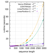
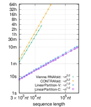
C

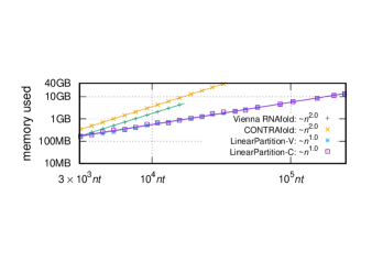
Figure 4: Total runtime and memory usage of computing both the partition function and base pairing probabilities. A: Runtime comparisons on the ArchiveII dataset; the curve-fittings were log-log in gnuplot with $n>10^{3}$. B: Runtime comparisons on the RNAcentral dataset (log scale). The partition function computation takes about half of the total time shown here. C: Memory usage comparisons on the RNAcentral dataset (log scale).

We present two versions of LinearPartition: LinearPartition-V using thermodynamic parameters ^{37, 38, 40} following Vienna RNAfold ³⁵, and LinearPartition-C using the learning-based parameters from CONTRAfold ²⁶. We use a Linux machine with 2.90GHz Intel i9-7920X CPU and 64G memory for benchmarks. We use sequences from two datasets, ArchiveII ^{37, 41} and RNAcentral ⁴². See B.1 for details of the datasets.

A

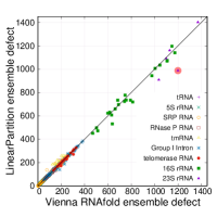
B

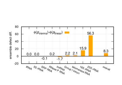
	C	D	E	F
E. coli 23S rRNA
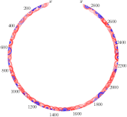
	G	H	I	J
C. ellipsoidea Group I Intron

Figure 5: A: Ensemble defect (expected number of incorrectly predicted nucleotides; lower is better) comparison between Vienna RNAfold and LinearPartition on the ArchiveII dataset. B: Ensemble defect difference for each family. LinearPartition has lower ensemble defects for longer families: on average 56.3 less incorrectly predicted nucleotides on 23S rRNA and 8.3 less over all families. C–F: An example of E. coli 23S rRNA (shaded point in A). C: Circular plot of the ground truth. D–F: Base pair probabilities from Vienna RNAplfold (with default window size $70$), RNAfold and LinearPartition, respectively; Blue denotes pairs in the known structure and Red denotes predicted pairs not in the known structure. The darkness of the line indicates pairing probability. G–J: Circular plots of C. ellipsoidea Group I Intron. See Fig. 6 for another view of this example.

Fig. 4 compares the efficiency and scalability between the two baselines, Vienna RNAfold and CONTRAfold, and our two versions, LinearPartition-V and LinearPartition-C. To make the comparison fair, we disable the downstream tasks (MEA prediction in CONTRAfold, and centroid prediction and visualization in RNAfold) which are by default enabled. Fig. 4A shows that both LinearPartition-V and LinearPartition-C scale almost linearly with sequence length $n$. The runtime deviation from exact linearity is due to the relatively short sequence lengths in the ArchiveII dataset, which contains a set of sequences with well-determined structures ⁴¹. Fig. 4A also confirms that the baselines scale cubically and the $O(n^{3})$ runtimes are substantially slower than LinearPartition on long sequences. For the H. pylori 23S rRNA sequence (2,968 nt, the longest in ArchiveII), both versions of LinearPartition take only 6 seconds, while RNAfold and CONTRAfold take 73 and 120 seconds, resp.

We also notice that both RNAfold and CONTRAfold have limitations on even longer sequences. RNAfold scales the magnitude of the partition function using a constant estimated from the minimum free energy of the given sequence to avoid overflow, but overflows still occur on long sequences. For example, it overflows on the 19,071 nt sequence in the sampled RNAcentral dataset. CONTRAfold stores the logarithm of the partition function to solve the overflow issue, but cannot run on sequences longer than 32,767 nt due to using unsigned short to index sequence positions. LinearPartition, like CONTRAfold, performs computations in the log-space, but can run on all sequences in the RNAcentral dataset. Fig. 4B compares the runtime of four systems on a sampled subset of RNAcentral dataset, and shows that on longer sequences the runtime of LinearPartition is exactly linear. For the 15,780 nt sequence, the longest example shown for RNAfold, LinearPartition-V is 256$\times$ faster (more than 3 hours vs. 44.1 seconds). Note that RNAfold may not overflow on some longer sequences, where LinearPartition-V should enjoy an even more salient speedup. For the longest sequence that CONTRAfold can run (32,753 nt) in the dataset, LinearPartition is 2,771$\times$ faster (2.5 days vs. 1.3 min.). Even for the longest sequence in RNAcentral (Homo Sapiens Transcript NONHSAT168677.1 with length 244,296 nt ⁴³), both LinearPartition versions finish in $\sim$10 minutes.

Fig. 4C shows that RNAfold and CONTRAfold use $O(n^{2})$ space while LinearPartition uses $O(n)$.

Now that we have established the speed of LinearPartition, we move on to the quality of its output.

3.2 Correlation with Ground Truth Structures

We use ensemble defect ⁴⁴ (Fig. 5A–B) to represent the quality of the Boltzmann distribution. It is the expected number of incorrectly predicted nucleotides over the whole ensemble at equilibrium, and formally, for a sequence $\mathbf{x}$ and its ground-truth structure $\mathbf{y}^{*}$, the ensemble defect is

$$\vspace{-0.2cm}\Phi(\mathbf{x},\mathbf{y}^{*})=\sum_{\mathbf{y}\in\mathcal{Y}(\mathbf{x})}p(\mathbf{y})\cdot d(\mathbf{y},\mathbf{y}^{*})$$ (1)

where $p(\mathbf{y})$ is the probability of structure $\mathbf{y}$ in the ensemble $\mathcal{Y(\mathbf{x})}$, and $d(\mathbf{y},\mathbf{y}^{*})$ is the distance between $\mathbf{y}$ and $\mathbf{y}^{*}$, defined as the number of incorrectly predicted nucleotides in $\mathbf{y}$:

$$\begin{split}d(\mathbf{y},\mathbf{y}^{*})=|\mathbf{x}|&-|\text{pairs}(\mathbf{y})\cap\text{pairs}(\mathbf{y}^{*})|\\ &-|\text{unpaired}(\mathbf{y})\cap\text{unpaired}(\mathbf{y}^{*})|\end{split}$$

The naïve calculation of Eq. 1 requires enumerating all possible structures in the ensemble, but by plugging $d(\mathbf{y},\mathbf{y}^{*})$ into Eq. 1 we have ⁴⁴

$$\vspace{-0.2cm}\begin{split}\Phi(\mathbf{x},\mathbf{y}^{*})=|\mathbf{x}|-2\!\!\sum_{(i,j)\in\text{pairs}(\mathbf{y}^{*})}p_{i,j}-\sum_{j\in\text{unpaired}(\mathbf{y}^{*})}q_{j}\end{split}\vspace{-0.2cm}$$

where $p_{i,j}$ is the probability of $i$ pairing with $j$ and $q_{j}$ is the probability of $j$ being unpaired, i.e., $q_{j}=1-\sum p_{i,j}$. This means we can now use base pairing probabilities to compute the ensemble defect.

A	B
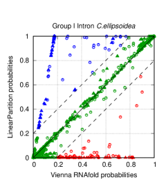
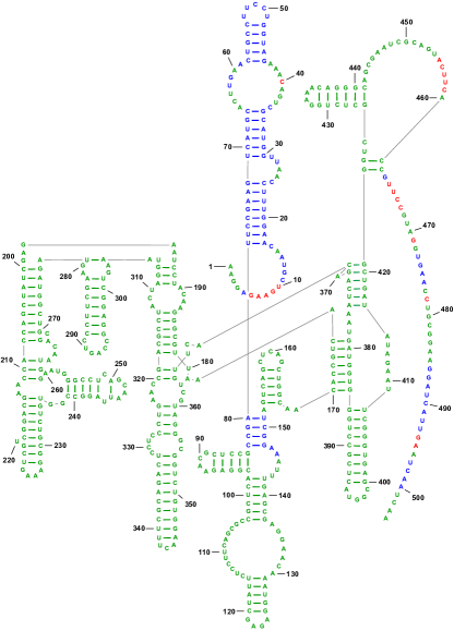
C

$p_{\mathrm{linear}}\!-\!p_{\mathrm{vienna}}\!>\!0.2$

$|p_{\mathrm{linear}}\!-\!p_{\mathrm{vienna}}|\!\leq\!0.2$

$p_{\mathrm{linear}}\!-\!p_{\mathrm{vienna}}\!<\!-0.2$

total		correct
55 $\blacktriangle$	40 $\circ$	23 $\blacktriangle$	37 $\circ$
126,645 $\blacktriangle$	420 $\circ$	111 $\blacktriangle$	180 $\circ$
56 $\blacktriangle$	44 $\circ$	0 $\blacktriangle$	19 $\circ$

Figure 6: A–C: An example of C. ellipsoidea Group I Intron. A: Solid triangles ( $\blacktriangle$ $\blacktriangle$ $\blacktriangle$) stand for base pairing probabilities and unfilled circles ( $\circ$ $\circ$ $\circ$) stand for single-stranded probabilities. blue: $p_{\mathrm{linear}}\!-\!p_{\mathrm{vienna}}\!>\!0.2$; green: $|p_{\mathrm{linear}}\!-\!p_{\mathrm{vienna}}|\!\leq\!0.2$; red: $p_{\mathrm{linear}}\!-\!p_{\mathrm{vienna}}\!<\!-0.2$; B: Ground truth structure colored with the above scheme; C: Statistics of this example. "total" columns are the total numbers of triangles and circles with different colors in A, while "correct" columns are the corresponding numbers in the ground-truth structure in B, which is better correlated with LinearPartition’s probabilities than Vienna RNAfold’s ( 23 blue pairs and 0 red pairs).

A	B	C	D
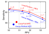
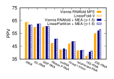
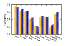
E	F	G	H

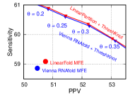
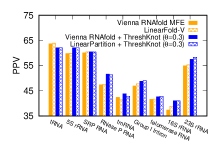
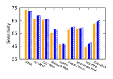
Figure 7: Accuracy of downstream predictions (MEA and ThreshKnot) using base pairing probabilities from Vienna RNAfold and LinearPartition on the ArchiveII dataset. A: Overall PPV-Sensitivity tradeoff of MFE (single point) and MEA with varying $\gamma$ (which can be tuned for higher sensitivity or PPV by adjusting $\gamma$). B & C: PPV and Sensitivity comparisons of MEA structures for each family. D: Accuracy comparison of long-distance base pairs (>500 nt apart) in the MEA structures. E–H: Same as A–D, but using ThreshKnot predictions instead of MEA. We conclude that MEA predictions based on LinearPartition-V are consistently better in both PPV and Sensitivity than those based on Vienna RNAfold for all $\gamma$’s, while ThreshKnot predictions based on those two are almost identical for all $\theta$’s. LinearPartition-V is substantially better on long-distance base pairs in both MEA and ThreshKnot predictions.

Fig. 5A–B employs ensemble defect to measure the average number of incorrectly predicted nucleotides over the whole ensemble (lower is better). Vienna RNAfold and LinearPartition have similar ensemble defects for short sequences, but LinearPartition has lower ensemble defects for longer sequences, esp. 16S and 23S rRNAs; in other words, LinearPartition’s ensemble has less expected number of incorrectly predicted nucleotides (or higher number of correctly predicted nucleotides). In particular, on 16S and 23S rRNAs, LinearPartition has on average 15.9 and 56.3 more correctly predicted nucleotides than RNAfold, and on average 8.3 more correctly predicted nucleotides over all families (Fig. 5B). Figs. SI 3 show the relative ensemble defects (normalized by sequence lengths), where the same observations hold, and LinearPartition has on avearge 0.4% more correctly predicted nucleotides over all families. In both cases, the differences on tmRNA (worse) and Group I Intron (better) are statistically significant ($p<0.01$).

This finding also implies that LinearPartition’s base pairing probabilities are on average higher than RNAfold’s for ground-truth base pairs, and on average lower for incorrect base pairs. We use two concrete examples to illustrate this. First, we plot the ground truth structure of E. coli 23S rRNA (2,904 nt) in Fig. 5C, and then plot the predicted base pairing probabilities from the local folding tool Vienna RNAplfold (with default window size 70), RNAfold, and LinearPartition in Fig. 5D–F, respectively. We can see that local folding can only produce local pairing probabilities, while RNAfold misses most of the long-distance pairs from the ground truth (except the 5’-3’ helix), and includes many incorrect long-distance pairings (shown in red). By contrast, LinearPartition successfully predicts many long-distance pairings that RNAfold misses, the longest being 582 nt apart (shown with arrows). Indeed, the ensemble defect of this example confirms that LinearPartition’s ensemble distribution has on average 211.4 more correctly predicted nucleotides (over 2,904 nt, or 7.3%) than RNAfold’s.

As the second example, we use C. ellipsoidea Group I Intron (504 nt). First, in Fig. 5G–J, we plot the circular plots in the same style as the previous example, where LinearPartition is substantially better in predicting 4 helices in the ground-truth structure: [17,24]–[72,79], [30,45]–[66,71], [44,48]–[54,58], and [80,83]–[148,151] (annotated with blue arrows). Next, in Fig. 6A, we plot the base pairs (in triangle) and unpaired bases (in circle) with RNAfold probability on x-axis and LinearPartition probability on y-axis. We color the circles and triangles in blue where LinearPartition gives 0.2 higher probability than RNAfold (top left region), the opposite ones (bottom right region) in red, and the remainder (diagonal region, with probability changes less than 0.2) in green. Then in Fig. 6B, we visualize the ground truth structure ⁴⁵ and color the bases as in Fig. 6A. We observe that the majority of bases are in green, indicating that RNAfold and LinearPartition agree with for a majority of the structure features. But the blue helices (near 5’-end and [80,83]–[148,151], see also Fig. 5J) indicate that LinearPartition favors these correct substructures by giving them higher probabilities than RNAfold. We also notice that all red features (where RNAfold does better than LinearPartition) are unpaired bases. This example shows that although LinearPartition and RNAfold give different probabilities, it is likely that LinearPartition prediction structure is closer to the ground truth structure (which will be confirmed by downstream structure predictions in Section 3.3). The ensemble defect of this example also confirms that LinearPartition has on average 47.1 more correctly predicted nucleotides (out of 504 nt, or 9.3%) than RNAfold.

Fig. 6C gives the statistics of this example. We can see the green triangles in Fig. 6A, which denote similar probabilities between RNAfold and LinearPartition, are the vast majority. The total number of blue triangles, for which LinearPartition gives higher base pairing probabilities, is 55, and among them 23 (41.8%) are in the ground truth structure. On the contrary, 56 triangles are in red, but none of these RNAfold prefered base pairs are correct. For unpaired bases, LinearPartition also gives higher probabilities to more ground truth unpaired bases: there are 40 blue circles, among which 37 (92.5%) are unpaired in the ground truth structure, while only 19 out of the 44 red circles (43.2%) are in the ground truth structure.

3.3 Accuracy of Downstream Predictions

An important application of the partition function is to improve structure prediction accuracy (over MFE) using base pairing probabilities. Here we use two such “downstream prediction” methods, MEA²⁶ and ThreshKnot ²⁹ which is a thresholded version of ProbKnot ²⁸, and compare their results using base pairing probabilities from $O(n^{3})$-time baselines and our $O(n)$-time LinearPartition. We use Positive Predictive Value (PPV, the fraction of predicted pairs in the known structure, a.k.a. precision) and sensitivity (the fraction of known pairs predicted, a.k.a. recall) as accuracy measurements for each family, and get overall accuracy be averaging over families. When scoring accuracy, we allow base pairs to differ by one nucleotide in position ³⁷. We compare RNAfold and LinearPartition-V on the ArchiveII dataset in the main text, and provide the CONTRAfold vs. LinearPartition-C comparisons in the Supporting Information Figs. SI 4–SI 5.

Fig. 7A shows MEA predictions (RNAfold + MEA and LinearPartition + MEA) are more accurate than MFE ones (RNAfold MFE and LinearFold-V), but more importantly, LinearPartition + MEA consistently outperforms RNAfold + MEA in both PPV and sensitivity with the same $\gamma$, a hyperparameter that balances PPV and sensitivity in MEA algorithm.

Figs. 7B–C detail the per-family PPV and sensitivity, respectively, for MFE and MEA ($\gamma=1.5$) results from Fig. 7A. LinearPartition + MEA has similar PPV and sensitivity as RNAfold + MEA on short families (tRNA, 5S rRNA and SRP), but interestingly, is more accurate on longer families, especially the two longest ones, 16S rRNA (+0.86 on PPV and +1.29 on sensitivity) and 23S rRNA (+0.88 on PPV and +0.62 on sensitivity).

ProbKnot is another downstream prediction method that is simpler and faster than MEA; it assembles base pairs with reciprocal highest pairing probabilities. Recently, we demonstrated ThreshKnot ²⁹, a simple thresholded version of ProbKnot that only includes pairs that exceed the threshold, leads to more accurate predictions that outperform MEA by filtering out unlikely pairs, i.e., those whose probabilities fall under a given threshold $\theta$.

Shown in Fig. 7E, LinearPartition + ThreshKnot is almost identical in overall accuracy to RNAfold + ThreshKnot at all $\theta$’s, and is slightly better than the latter on long families (+0.24 on PPV and +0.38 on sensitivity for Group I Intron, +0.12 and +0.37 for telomerase RNA, and +0.74 and +0.62 for 23S rRNA) (Figs. 7F–G). We also performed a two-tailed permutation test to test the statistical significance, and observed that on tmRNA, both MEA and ThreshKnot structures of LinearPartition are significantly worse ($p\!<\!0.01$) than their RNAfold-based counterparts in both PPV and Sensitivity.

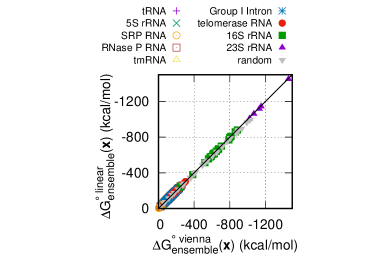
A	B
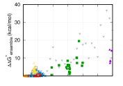
	C

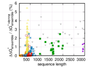
Figure 8: Approximation quality of partition function on ArchiveII dataset and random sequences. A: The x and y axes are ensemble folding free energy changes $\Delta G^{\circ}_{\text{ensemble}}(\mathbf{x})$ of Vienna RNAfold and LinearPartition, respectively. B: Difference of ensemble folding free energy change (top), ${\Delta\Delta G^{\circ}_{\text{ensemble}}(\mathbf{x})}$, between RNAfold and LinearPartition. and the relative differences (bottom), ${\Delta\Delta G^{\circ}_{\text{ensemble}}(\mathbf{x})}/{\Delta G^{\circ\ \text{vienna}}_{\text{ensemble}}(\mathbf{x})}$, in percentages.

Fig. 7D & H show that LinearPartition-based predictions are subtantially better than RNAfold’s (in both PPV and sensitivity) for long-distance base pairs (those with 500+ nt apart), which are well known to be challenging for the current models. Fig. SI 6 details the accuracies on base pairs with different distance groups.

Figs. SI 4–SI 5 show similar comparisons between CONTRAfold and LinearPartition-C using MEA and ThreshKnot prediction, with similar results to Fig. 7, i.e., downstream structure prediction using LinearPartition-C is as accurate as using CONTRAfold, and (sometimes significantly) more accurate on longer families.

A	B	E
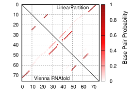
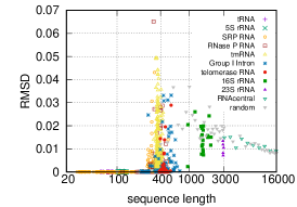
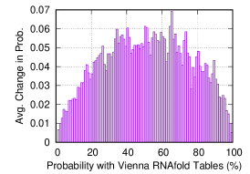
C	D	F

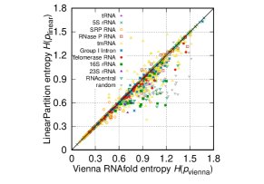
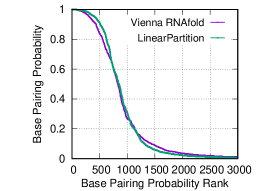
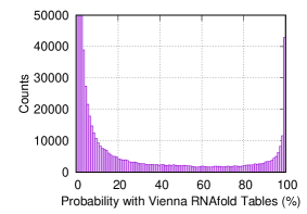
Figure 9: Comparison of base pairing probabilities from Vienna RNAfold and LinearPartition. A: LinearPartition (upper triangle) and Vienna RNAfold (lower triangle) result in identical base pairing probability matrix for E. coli tRNA${}^{\textit{Gly}}$. B: The root-mean-square deviation, $\text{\sc rmsd}(p_{\mathrm{vienna}},p_{\mathrm{linear}})$, is relatively small between LinearPartition and Vienna RNAfold; all tRNA and 5S rRNA sequences rmsd is close to 0 (e.g., RMSD$<10^{-5}$). C: Average positional structural entropy $H(p)$ comparison; LinearPartition has noticeably lower entropy. D: LinearPartition starts higher and finishes lower than Vienna RNAfold in a sorted probability curve for E. coli 23S rRNA, suggesting lower entropy. E: Mean absolute value of change in base pairing probabilities between Vienna RNAfold and LinearPartition; these changes are averaged within every probability bin. F: Pair probability distribution of Vienna RNAfold. Note that the y-axis is limited to 50,000 counts, and the counts of first three bins (with probability smaller than 3%) are far beyond 50,000.

3.4 Approximation Quality (Default Beam Size)

LinearPartition uses beam pruning to ensure $O(n)$ runtime, thus is approximate compared with standard $O(n^{3})$-time algorithms. We now investigate its approximation quality at the default beam size 100.

First, in Fig. 8, we measure the approximation quality of the partition function calculation, in particular, the ensemble folding free energy change (also known as “free energy of the ensemble”) which reflects the size of the partition function,

$$\Delta G^{\circ}_{\text{ensemble}}(\mathbf{x})=-RT\log Q(\mathbf{x}).$$

Fig. 8A shows that the LinearPartition estimate for the ensemble folding free energy change is close to the RNAfold estimate on the ArchiveII dataset and randomly generated RNA sequences. The similarity shows that little magnitude of the partition function is lost by the beam pruning. For short families, free energy of ensembles between LinearPartition and RNAfold are almost the same. For 16S and 23S rRNA sequences and long random sequences (longer than 900 nucleotides), LinearPartition gives a lower magnitude ensemble free energy change, but the difference,

$$\Delta\Delta G^{\circ}_{\text{ensemble}}(\mathbf{x})=\Delta G^{\circ\ \text{vienna}}_{\text{ensemble}}(\mathbf{x})-\Delta G^{\circ\ \text{linear}}_{\text{ensemble}}(\mathbf{x})\,\geq 0$$

is smaller than 20 kcal/mol for 16S rRNA, 15 kcal/mol for 23S rRNA, and 37 kcal/mol for random sequences (Fig. 8B). The maximum difference for random sequence is larger than natural sequences (by 17.2 kcal/mol). This likely reflects the fact that random sequences tend to fold less selectively to probable structures ⁴⁶, and the beam is therefore pruning structures in random that would contribute to the overall folding stability. Fig 8C shows the “relative” differences in ensemble free energy changes, ${\Delta\Delta G^{\circ}_{\text{ensemble}}(\mathbf{x})}/{\Delta G^{\circ\ \text{vienna}}_{\text{ensemble}}(\mathbf{x})}$, are also very small: only up to 2.5% and 1.5% for 16S and 23S rRNAs, and up to 4.5% for random sequences.

Next, in Fig. 9, we measure the approximation quality of base pairing probabilities using root-mean-square deviation (rmsd) between two probability matrices $p$ and $p^{\prime}$ over the set of all possible Watson-Crick and wobble pairs on a sequence $\mathbf{x}$. We define

$$\vspace{-0.4cm}\begin{split}{\text{pairings}}(\mathbf{x})\!=\!\{&1\leq i<j\leq|\mathbf{x}|\bigm{|}j-i>3\\[-2.84544pt] &\mathbf{x}_{i}\mathbf{x}_{j}\in\{\text{\small CG, GC, AU, UA, GU, UG}\}\!\}\end{split}$$

and:

$$\text{\sc rmsd}(p,p^{\prime})\!=\!\!\!\sqrt{\frac{1}{|{\text{pairings}}(\mathbf{x})|}\sum_{(i,j)\in{{\text{pairings}}(\mathbf{x})}}{\!\!\!\!\!(p_{i,j}\!-\!p^{\prime}_{i,j})}^{2}}$$

A

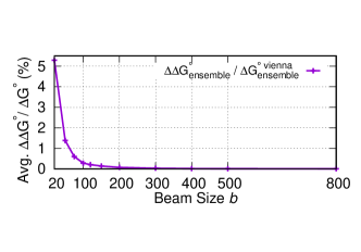
B

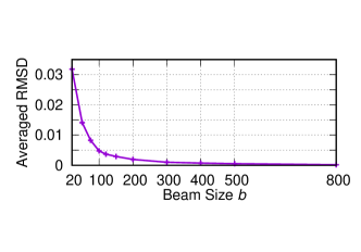
C

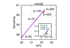
D

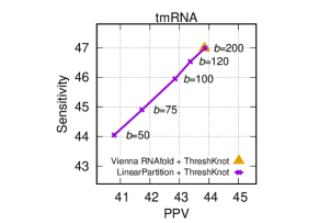
E

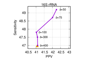
Figure 10: Impact of beam size. A: Relative difference of ensemble folding free energy change, $\Delta\Delta G^{\circ}_{\text{ensemble}}/\Delta G^{\circ}_{\text{ensemble}}$, against beam size. B: RMSD against beam size. C: Overall PPV and Sensitivity with beam size. D–E: tmRNA and 16S rRNA PPV and Sensitivity against beam size, respectively. Note that the results of ThreshKnot using RNAfold (yellow triangles in C–E) are identical to ThreshKnot using the exact version of LinearPartition ($b\!=\!\infty$).

Figs. 9A and B confirm that our LinearPartition algorithm (with default beam size 100) can indeed approximate the base pairing probability matrix reasonably well. Fig. 9A shows the heatmap of probability matrices for E. coli tRNA${}^{\textit{Gly}}$. RNAfold (lower triangle) and LinearPartition (upper triangle) yield identical matrices (i.e., $\text{\sc rmsd}=0$). Fig. 9B shows that the rmsd of each sequence in ArchiveII and RNAcentral datasets, and randomly generated artificial RNA sequences, is relatively small. The highest deviation is 0.065 for A. truei RNase P RNA, which means on average each base pair’s probability deviation in that worst-case sequence is about 0.065 between the cubic algorithm (RNAfold) and our linear-time one (LinearPartition). On the longest 23S rRNA family, the rmsd is about 0.015. We notice that tmRNA is the family with biggest average rmsd. The random RNA sequences behave similarly to natural sequences in terms of rmsd, i.e., rmsd is close to 0 ($\!<\!10^{-5}$) for short ones, then becomes bigger around length 500 and decreases after that, but for most cases their rmsd’s are slightly larger than the natural sequences. This indicates that the approximation quality is relatively better for natural sequences. For RNAcentral-sampled sequences, rmsd’s are all small and around 0.01.

We hypothesize that LinearPartition reduces the uncertainty of the output distributions because it filters out states with lower partition function. We measure this using average positional structural entropy $H(p)$, which is the average of positional structural entropy $H_{2}(i)$ for each nucleotide $i$ ^{47, 48}:

$$\vspace{-0.3cm}\begin{split}H(p)&=\frac{1}{n}\sum_{i=1}^{n}{H_{2}(i)}=\frac{1}{n}\sum_{i=1}^{n}({-\sum_{j=0}^{n}p_{i,j}\mathrm{log}_{2}p_{i,j}})\\ &=-\frac{1}{n}\sum_{i=1}^{n}{\sum_{j=0}^{n}p_{i,j}\mathrm{log}_{2}p_{i,j}}\end{split}$$

where $p$ is the base pairing probability matrix, and $p_{i,0}$ is the probability of nucleotide $i$ being unpaired ($q_{i}$ in Eq. 1). The lower entropy indicates that the distribution is dominated by fewer base pairing probabilities. Fig. 9C confirms LinearPartition distribution shifted to higher probabilities (lower average entropy) than RNAfold for most sequences.

Fig. 9D uses E. coli 23S rRNA to exemplify the difference in base pairing probabilities. We sort all these probabilities from high to low and take the top 3,000. The LinearPartition curve starts higher and finishes lower, confirming a lower entropy.

Figs. 9E and F follow a previous analysis method ⁴⁹ to estimate the approximation quality with a different perspective. We divide the base pairing probabilities range [0,1] into 100 bins, i.e., the first bin is for base pairing probabilities [0,0.01), and the second is for [0.01, 0.02), so on so forth. In Fig. 9E we visualize the averaged change of base pairing probabilities between RNAfold and LinearPartition for each bin. We can see that larger probability changes are in the middle (bins with probability around 0.5), and smaller changes on the two sides (with probability close to either 0 or 1). In Fig. 9F we illustrate the counts in each bin based on RNAfold base pairing probabilities. We can see that most base pairs have low probabilities (near 0) or very high probabilities (near 1). Combine Figs. 9E and F together, we can see that probabilities of most base pairs are near 0 or 1, where the differences between RNAfold and LinearPartition are relatively small. Fig. SI 7 provides the comparison of counts in each bin between RNAfold and LinearPartition-V. The count of LinearPartition-V in bin [99,100) is slightly higher than RNAfold, while the counts in bins near 0 (being capped at 50,000) are much less than RNAfold. This also confirms that LinearPartition prunes base pairs with tiny probabilities.

3.5 Adjustable Beam Size

Beam size in LinearPartition is a user-adjustable hyperparameter controlling beam prune, and it balances the approximation quality and runtime. A smaller beam size shortens runtime, but sacrifices approximation quality. With increasing beam size, LinearPartition gradually approaches the classical $O(n^{3})$-time algorithm and the output is finally identical to the latter when the beam size is $\infty$ (no pruning). Fig. 10A shows the changes in approximation quality of the ensemble free energy change, $\Delta G^{\circ}_{\text{ensemble}}(\mathbf{x})$, with $b=20\rightarrow 800$. Even with a small beam size ($b=20$) the difference is only about 5%, which quickly shrinks to 0 as $b$ increases. Fig. 10B shows the changes in rmsd with changing $b$. With a small beam size $b=20$ the average rmsd is lower than 0.035 over all ArchiveII sequences, which shrinks to less than 0.005 at the default beam size ($b=100$), and almost 0 with $b=500$.

Beam size also has impact on PPV and Sensitivity. Fig. 10C gives the overall PPV and Sensitivity changes with beam size. We can see both PPV and Sensitivity improve from $b=50$ to $b=100$, and then become stable beyond that. Figs. 10D and E present this impact for two selected families. Fig. 10D shows tmRNA’s PPV and Sensitivity both increase when enlarging beam size. Using beam size 200, LinearPartition achieves similar PPV and Sensitivity as RNAfold. However, increasing beam size is not benefical for all families. Fig. 10E gives the counterexample of 16S rRNA. We can see both PPV and Sensitivity decrease with $b$ from 50 to 100. After that, Sensitivity drops with no PPV improvement.

LinearFold uses $k$-best parsing ⁵⁰ to reduce runtime from $O(nb^{2})$ to $O(nb{\mathrm{log}}b)$ without losing accuracy. Basically, $k$-best parsing is to find the exact top-$k$ (here $k\!=\!b$) states out of $b^{2}$ candidates in $O(b{\mathrm{log}}b)$ runtime. If we applied $k$-best parsing here, LinearPartition would sum the partition function of only these top-$b$ states instead of the partition function of $b^{2}$ states. This change would introduce a larger approximation error, especially when the differences of partition function between the top-$b$ states and the following states near the pruning boundary are small. Therefore, in LinearPartition we do not use $k$-best parsing as in LinearFold, and the runtime is $O(nb^{2})$ instead of $O(nb\log b)$.

Finally, we note that the default beam size $b\!=\!100$ follows LinearFold and we do not tune it.

4 Discussion

4.1 Summary

The classical McCaskill (1990) algorithm for partition function and base pairing probabilities calculations are widely used in many studies of RNA sequences, but its application has been impossible for long sequences (such as full length mRNA) due to its cubic runtime. To address this issue, we present LinearPartition, a linear-time algorithm that dramatically reduces the runtime without sacrificing output quality. We confirm that:

1. LinearPartition takes only linear runtime and memory usage, and is orders of magnitude faster on longer sequences (Fig. 4);

2. The base pairing probabilities produced by LinearPartition are better correlated with the ground truth structures on average (Figs. 5–6);

3. When used with downstream structure prediction methods such as MEA and ThreshKnot, LinearPartition’s base pair probabilities have similar overall accuracy (or even a small improvement on MEA structures) compared with RNAfold, as well as better accuracies on longer families and long-distance base pairs (Fig. 7);

4. LinearPartition has a reasonable approximation quality (Figs. 8–9) in terms of rmsd.

There are two possible reasons why our approximation results in better base pairing probabilities:

1. This is consistent with the findings in LinearFold, where approximate folding via beam search yields more accurate structures.

2. LinearPartition’s pruning of low-probability (sub)structures has a “regularization” effect. It eliminates some noise in the current energy model which is highly inaccurate, especially for long-distance interactions.

The success of LinearPartition is arguably more striking than LinearFold, since the former needs to sum up exponentially many structures that capture the bulk part of the ensemble free energy, while the latter only needs to find one single optimal structure.

4.2 Extensions

Our work has potential extensions.

1. Existing methods and tools for bimolecular and multistrand base pairing probabilities as well as accessibility computation ^{51, 52, 53, 54} are rather slow, which limits their applications on long sequences. LinearPartition will likely provide a much faster solution for these problems.

2. We will linearize the partition function-based heuristic methods for pseudoknot prediction such as IPknot and Dotknot. These heuristic methods use rather simple criteria to choose pairs from the base pairing probability matrix, and their runtime bottleneck is $O(n^{3})$-time calculation of the base pairing probabilities. With LinearPartition we can overcome the costly bottleneck and get an overall much faster tool.

3. We can also speed up stochastic sampling of RNA secondary structures from Boltzmann distribution. The standard stochastic sampling algorithm runs in worst-case $O(n^{2})$ time ³², but relies on the classical $O(n^{3})$ partition function calculation. With LinearPartition, we can apply stochastic sampling to full length sequences such as mRNAs, and compute their accessbility based on sampled structures.

References

Supporting Information
LinearPartition: Linear-Time Approximation of RNA Folding Partition Function and Base Pairing Probabilities
He Zhang, Liang Zhang, David H. Mathews and Liang Huang

Appendix A Details of the Efficient Implementation

A.1  Data Structures

In the main text, for simplicity of presentation, $Q$ is described as a hash from span $[i,j]$ to $Q_{{{i}},{{j}}}$, but in our actual implementation, to make sure the overall runtime is $O(nb^{2})$, we implement $Q$ as an array of $n$ hashes, where each $Q[j]$ is a hash mapping $i$ to $Q[j][i]$ which is conveniently notated as $Q_{{{i}},{{j}}}$ in the main text. It is important to note that the first dimension $j$ is the right boundary and the second dimension $i$ is the left boundary of the span $[i,j]$. See the following table for a summary of notations and the corresponding actual implementations. Here we use Python notation for simplicity, but in actual system we implement with C++.

notations in this paper	Python implementation
$Q\leftarrow$ hash()	Q = [defaultdict(float) for _ in range(n)]
$Q_{{{i}},{{j}}}$	Q[j][i]
$[i,j]$ in $Q$	i in Q[j]
for each $i$ such that $[i,j]$ in $Q$	for i in Q[j]
delete $[i,j]$ from $Q$	del Q[j][i]

A.2  Complexity Analysis

In the partition function calculation (inside phase) in Fig. 3, the number of states is $O(nb)$ because each $Q[j]$ contains at most $b$ states ($Q_{{{i}},{{j}}}$’s) after pruning. Therefore the space complexity is $O(nb)$. For time complexity, there are three nested loops, the first one ($j$) with $n$ iterations, the second ($i$) and the third ($k$) loops both have $O(b)$ iterations thanks to pruning, so the overall runtime is $O(nb^{2})$.

A.3  Outside Partition Function and Base Pairing Probability Calculation

After we compute the partition functions $Q_{{{i}},{{j}}}$ on each span $[i,j]$ (known as the “inside partition function”), we also need to compute the complementary function $\widehat{Q}_{{{i}},{{j}}}$ for each span known as the “outside partition function” in order to derive the base-pairing probabilities. Unlike the inside phase, this outside partition function is calculated from top down, with $\widehat{Q}_{{{1}},{{n}}}=1$ as the base case.

$$\begin{split}\widehat{Q}_{{{i}},{{j}}}&=\widehat{Q}_{{{i}},{{j+1}}}\cdot e^{-\frac{\delta(\mathbf{x},j+1)}{RT}}\\ &+\sum_{k<i}\widehat{Q}_{{{k}},{{j+1}}}\cdot Q_{{{k}},{{i-2}}}\cdot e^{-\frac{\xi(\mathbf{x},i-1,j+1)}{RT}}\\ &+\sum_{k>j+1}\widehat{Q}_{{{i}},{{k}}}\cdot Q_{{{j+2}},{{k-1}}}\cdot e^{-\frac{\xi(\mathbf{x},j+1,k)}{RT}}\end{split}$$

Note that the second line is only possible when $x_{i-1}x_{j+1}$ can form a base pair (otherwise $e^{-\frac{\xi(\mathbf{x},i-1,j+1)}{RT}}=0$) and the third line has a constraint that $x_{j+1}x_{k}$ can form a base pair (otherwise $e^{-\frac{\xi(\mathbf{x},j+1,k)}{RT}}=0$).

For each $(i,j)$ where $x_{i}x_{j}$ can form a base pair, we compute its pairing probability:

$$p_{i,j}=\sum_{k\leq i}\widehat{Q}_{{{k}},{{j}}}\cdot Q_{{{k}},{{i-1}}}\cdot e^{-\frac{\xi(\mathbf{x},i,j)}{RT}}\cdot Q_{{{i+1}},{{j-1}}}$$

The whole “outside” computation takes $O(n^{3})$ without pruning, but also $O(nb^{2})$ with beam pruning. See Fig. SI 2 for the pseudocode to compute the outside partition function and base pairing probabilities.

Appendix B Details of datasets, baselines and methods

B.1  Datasets

We use sequences from two datasets, ArchiveII and RNAcentral. The archiveII dataset (available in http://rna.urmc.rochester.edu/pub/archiveII.tar.gz) is a diverse set with 3,857 RNA sequences and their secondary structures. It is first curated in the 1990s to contain sequences with structures that were well-determined by comparative sequence analysis ³⁷and updated later with additional structures ⁴¹. We remove 957 sequences that appear both in the ArchiveII and the S-Processed datasets ⁵⁵, because CONTRAfold uses S-Processed for training. We also remove all 11 Group II Intron sequences because there are so few instances of these that are available electronically. Additionally, we removed 30 sequences in the tmRNA family because the annotated structure for each of these sequences contains fewer than 4 pseudoknots, which suggests the structures are incomplete. These preprocessing steps lead to a subset of ArchiveII with 2,859 reliable secondary structure examples distributed in 9 families. See SI 1 for the statistics of the sequences we use in the ArchiveII dataset. Moreover, we randomly sampled 22 longer RNA sequences (without known structures) from RNAcentral ⁴² (https://rnacentral.org/), with sequence lengths ranging from 3,048 nt to 244,296 nt. For the sampling, we evenly split the range from $3,000$ to $244,296$ (the longest) into 24 bins by log-scale, and for each bin we randomly select a sequence (there are bins with no sequences).

To show the approximation quality on random RNA sequences, we generated 30 sequences with uniform distribution over {A, C, G, U}. The lengths of these sequences are spaced in 100 nucleotide intervals from 100 to 3,000.

	# of seqs		length
Family	total	used	avg	max	min
tRNA	557	74	77.3	88	58
5S rRNA	1,283	1,125	118.8	135	102
SRP RNA	928	886	186.1	533	28
RNase P RNA	454	182	344.1	486	120
tmRNA	462	432	369.1	433	307
Group I Intron	98	96	424.9	736	210
Group II Intron	11	0	-	-	-
telomerase RNA	37	37	444.6	559	382
16S rRNA	22	22	1,547.9	1995	950
23S rRNA	5	5	2,927.4	2968	2904
Overall	3,846	2,859	221.1	2968	28

Table SI 1: Statistics of the sequences in the ArchiveII dataset used in this work.

B.2  Baseline Software

We use two baseline software packages: (1) Vienna RNAfold (Version 2.4.11) from https://www.tbi.univie.ac.at/RNA/download/sourcecode/2_4_x/ViennaRNA-2.4.11.tar.gz and (2) CONTRAfold (Version 2.0.2) from http://contra.stanford.edu/. Vienna RNAfold is a widely-used RNA structure prediction package, while CONTRAfold is a successful machine learning-based RNA structure prediction system. Both provide partition function and base pairing probability calculations based on the classical cubic runtime algorithm. Our comparisons mainly focus on the systems with the same model, i.e., LinearPartition-V vs. Vienna RNAfold and LinearPartition-C vs. CONTRAfold. In this way the differences are based on algorithms themselves rather than models. We found a bug in CONTRAfold by comparing our results to CONTRAfold, which led to overcounting multiloops in the partition function calculation. We corrected the bug, and all experiments are based on this bug-fixed version of CONTRAfold.

B.3  Evaluation Metrics and Significance Test

Due to the uncertainty of base-pair matches existing in comparative analysis and the fact that there is fluctuation in base pairing at equilibrium, we consider a base pair to be correctly predicted if it is also displaced by one nucleotide on a strand ³⁷. Generally, if a pair $(i,j)$ is in the predicted structure, we consider it a correct prediction if one of $(i,j)$, $(i-1,j)$, $(i+1,j)$, $(i,j-1)$, $(i,j+1)$ is in the ground truth structure.

We use Positive Predictive Value (PPV) and sensitivity as accuracy measurements. Formally, denote $\mathbf{y}$ as the predicted structure and $\mathbf{y}^{*}$ as the ground truth, we have:

$$\text{PPV}=\frac{\#_{\text{TP}}}{\#_{\text{TP}}+\#_{\text{FP}}}=\frac{|\text{pairs}(\mathbf{y})\cap\text{pairs}(\mathbf{y}^{*})|}{|\text{pairs}(\mathbf{y})|}$$

$$\text{Sensitivity}=\frac{\#_{\text{TP}}}{\#_{\text{TP}}+\#_{\text{FN}}}=\frac{|\text{pairs}(\mathbf{y})\cap\text{pairs}(\mathbf{y}^{*})|}{|\text{pairs}(\mathbf{y}^{*})|}$$

where $\#_{\text{TP}}$ is the number of true positives (correctly predicted pairs), $\#_{\text{FP}}$ is the number of false positives (wrong predicted pairs) and $\#_{\text{FN}}$ is the number of false negatives (missing ground truth pairs).

We test statistical significance using a paired, two-sided permutation test ⁵⁶. We follow the common practice, choosing $10,000$ as the repetition number and $\alpha=0.05$ as the significance threshold.

B.4  Curve Fitting

We determine the best exponent $a$ for the scaling curve $O(n^{a})$ for each data series in Figures 2 and 4. Specifically, we use $f(x)=ax+b$ to fit the log-log plot of those series in Gnuplot; e.g., fitting $\log t_{n}=a\log n+b$, where $t_{n}$ is the running time on a sequence of length $n$, so that $t_{n}=e^{b}n^{a}$. Gnuplot uses the nonlinear least-squares Marquardt-Levenberg algorithm.

Appendix C Supporting Figures

1:function beamprune($Q,j,b$)

2:    $\mathit{candidates}\leftarrow$ hash() $\triangleright$ hash table: from candidates $i$ to score

3:    for each $i$ such that $[i,j]$ in $Q$ do

4:         $\mathit{candidates}[i]\leftarrow Q_{{{1}},{{i-1}}}\cdot Q_{{{i}},{{j}}}$ $\triangleright$ like LinearFold, use $Q_{{{1}},{{i-1}}}$ as prefix score     

5:    $\mathit{candidates}\leftarrow\textsc{SelectTopB}(candidates,b)$ $\triangleright$ select top-$b$ states by score

6:    for each $i$ such that $[i,j]$ in $Q$ do

7:         if key $i$ not in $candidates$ then

8:             delete $[i,j]$ from $Q$ $\triangleright$ prune low-scoring states              

Figure SI 1: The BeamPrune function from the Pseudocode of our main algorithm (Fig. 3).

x

1:function BasePairingProbs($\mathbf{x},Q$) $\triangleright$ outside calculation

2:    $n\leftarrow$ length of $\mathbf{x}$

3:    $\widehat{Q}\leftarrow$ hash() $\triangleright$ hash table: from span $[i,j]$ to $\widehat{Q}_{{{i}},{{j}}}$: outside partition function

4:    $p\leftarrow$ hash() $\triangleright$ hash table: from span $[i,j]$ to $p_{i,j}$: base-pairing probs

5:    $\widehat{Q}_{{{1}},{{n}}}\leftarrow 1$ $\triangleright$ base case

6:    for $j=n$ downto $1$ do

7:         for each $i$ such that $[i,\,j-1]$ in $Q$ do

8:             $\widehat{Q}_{{{i}},{{j-1}}}\mathrel{+}=\widehat{Q}_{{{i}},{{j}}}\cdot e^{-\frac{\delta(\mathbf{x},j)}{RT}}$ $\triangleright$ skip

9:             if $x_{i-1}x_{j}$ in {AU, UA, CG, GC, GU, UG} then

10:                 for each $k$ such that $[k,\,i-2]$ in $Q$ do

11:                     $\widehat{Q}_{{{k}},{{i-2}}}\mathrel{+}={\widehat{Q}_{{{k}},{{j}}}\cdot Q_{{{i}},{{j-1}}}\cdot e^{-\frac{\xi(\mathbf{x},i-1,j)}{RT}}}$ $\triangleright$ pop: left

12:                     $\widehat{Q}_{{{i}},{{j-1}}}\mathrel{+}={\widehat{Q}_{{{k}},{{j}}}\cdot Q_{{{k}},{{i-2}}}\cdot e^{-\frac{\xi(\mathbf{x},i-1,j)}{RT}}}$ $\triangleright$ pop: right

13:                     $p_{i-1,\,j}\mathrel{+}=\displaystyle\frac{\widehat{Q}_{{{k}},{{j}}}\cdot Q_{{{k}},{{i-2}}}\cdot e^{-\frac{\xi(\mathbf{x},i-1,j)}{RT}}\cdot Q_{{{i}},{{j-1}}}}{Q_{{{1}},{{n}}}}$ $\triangleright$ accumulate base pairing probs                                            

14:    return $p$ $\triangleright$ return the (sparse) base-pairing probability matrix

Figure SI 2: Outside partition function and base pairing probabilities calculation for a simplified version of the LinearPartition. $Q$ is the (inside) partition function calculated by the pseudocode in Fig. 3, and $\widehat{Q}$ is the outside partition function. The actual algorithm using the Turner model is in our GitHub codebase.

A	B

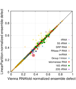
Figure SI 3: The comparison of normalized ensemble defects (normalized by sequence length) on the ArchiveII dataset. A: Normalized ensemble defect between Vienna RNAfold and LinearPartition-V for each sequence; the trend is similar as Fig. 5A, but the deviations for tmRNAs are more apparent; the point with red shaded are the example in Fig. 6. B: Normalized ensemble defect difference for each family; for longer families, e.g., Group I Intron, telomerase RNA, 16S and 23S rRNA, LinearPartition has lower normalized ensemble defect differences; note that LinearPartition’s normalized ensemble defects are significantly better than Vienna RNAfold on Group I Intron ($p<0.01$), but significantly worse on tmRNA ($p<0.01$).

A	B

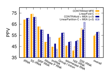
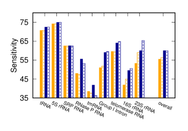
Figure SI 4: Accuracy comparison of MEA structures ($\gamma=3$) between CONTRAfold and LinearPartition-C on the ArchiveII dataset. $\gamma$ is the hyperparameter balances PPV and Sensitivity. Note that LinearPartition-C + MEA is significantly worse than CONTRAfold + MEA on two families in both PPV and Sensitivity, tmRNA and RNase P RNA ($p<0.01$).

A	B

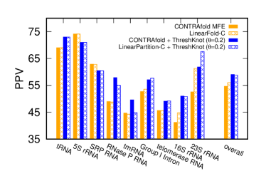
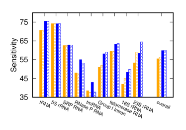
Figure SI 5: Accuracy comparison of ThreshKnot structure ($\theta=0.2$) between CONTRAfold and LinearPartition-C on ArchiveII dataset. $\theta$ is the hyperparameter that balances PPV and Sensitivity. Note that LinearPartition-C + ThreshKnot is significantly worse than CONTRAfold + ThreshKnot on two families in both PPV and Sensitivity, tmRNA and RNase P RNA ($p<0.01$), and significantly better on three longer families in Sensitivity, Group I Intron ($p<0.01$), telomerase RNA and 16S rRNA ($0.01\leq p<0.05$).

A	B
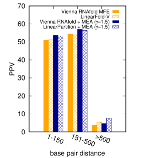
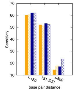
C	D

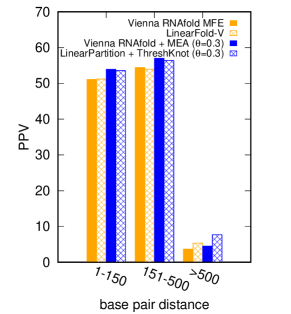
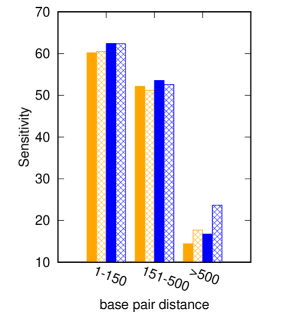
Figure SI 6: Accuracy comparison of base pair prediction with different base pair distances. Each bar represents the overall PPV/sensitivity of all predicted base pairs in a certain length range across all sequences. LinearPartition performs best on long base pairs over four systems. A and B: Comparison using MEA structures. C and D: Comparison using ThreshKnot structures. In all cases, LinearPartition’s base pair probabilities lead to substantially better accuracies on long-distance pairs (500+ nt apart).

A	B

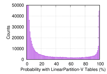
Figure SI 7: Pair probability distributions of Vienna RNAfold and LinearPartition-V are similar. A: Pair probability distribution of Vienna RNAfold; B: Pair probability distribution of LinearPartition-V. The count of LinearPartition-V in bin [99,100) is slightly bigger than Vienna RNAfold, while the count in bin [0,1) (cut here at 50,000) is much less than Vienna RNAfold (2,068,758 for LinearPartition-V and 48,382,357 for Vienna RNAfold).

References

- [1] Eddy. SR (2001) Non-coding RNA genes and the modern RNA world. Nature Reviews Genetics 2(12):919–929.
- [2] Doudna JA, Cech TR (2002) The chemical repertoire of natural ribozymes. Nature 418(6894):222–228.
- [3] Bachellerie JP, Cavaillé J, Hüttenhofer A (2002) The expanding snoRNA world. Biochimie 84(8):775–790.
- [4] Zhang J, Ferré-D’Amaré AR (2014) New molecular engineering approaches for crystallographic studies of large RNAs. Curr. Opin. Struct. Biol. 26:9—15.
- [5] Zhang H, Keane S (2019) Advances that facilitate the study of large RNA structure and dynamics by nuclear magnetic resonance spectroscopy. Wiley Interdisciplinary Reviews: RNA 10:e1541.
- [6] Lyumkis D (2019) Challenges and opportunities in cryo-EM single-particle analysis. Journal of Biological Chemistry 294(13):5181–5197.
- [7] Miao Z, , et al. (2017) RNA-puzzles round III: 3D RNA structure prediction of five riboswitches and one ribozyme. RNA 23(5):655–672.
- [8] Tinoco I, Bustamante. C (1999) How RNA folds. J. Mol. Biol. 293(2):271–281.
- [9] Flores SC, Altman RB (2010) Turning limited experimental information into 3d models of RNA. RNA 16(9):1769–1778.
- [10] Seetin MG, Mathews DH (2011) Automated RNA tertiary structure prediction from secondary structure and low-resolution restraints. J. Comp. Chem. 32(10):2232–2244.
- [11] Zuker M, Stiegler P (1981) Optimal computer folding of large RNA sequences using thermodynamics and auxiliary information. NAR 9(1):133–148.
- [12] McCaskill JS (1990) The equilibrium partition function and base pair probabilities for RNA secondary structure. Biopolymers 29:1105–19.
- [13] Lange S, et al. (2012) Global or local? predicting secondary structure and accessibility in mRNAs. NAR 40(12):5215–5226.
- [14] Bernhart SH, Hofacker IL, Stadler PF (2006) Local RNA base pairing probabilities in large sequences. Bioinformatics 22(5):614–615.
- [15] Kiryu H, Kin T, Asai K (2008) Rfold: an exact algorithm for computing local base pairing probabilities. Bioinformatics 24(3):367–373.
- [16] Huang L, et al. (2019) LinearFold: linear-time approximate RNA folding by 5’-to-3’ dynamic programming and beam search. Bioinformatics 35(14):i295–i304.
- [17] Cordero P, Das R (2015) Rich RNA structure landscapes revealed by mutate-and-map analysis. PLOS Computational Biology 11(11).
- [18] Lyngsø RB, Pedersen CNS (2000) RNA pseudoknot prediction in energy-based models. J. Comp. Biol. 7(3/4):409–427.
- [19] Nussinov R, Jacobson AB (1980) Fast algorithm for predicting the secondary structure of single-stranded RNA. PNAS 77(11):6309–6313.
- [20] Mathews. DH (2004) Using an RNA secondary structure partition function to determine confidence in base pairs predicted by free energy minimization. RNA 10(8):1178–1190.
- [21] Long D, , et al. (2007) Potent effect of target structure on microRNA function. Nat. Struct. Mol. Biol. 14(4):287–294.
- [22] Lu ZJ, Mathews DH (2008) Efficient siRNA selection using hybridization thermodynamics. NAR 36:640–647.
- [23] Tafer H, et al. (2008) The impact of target site accessibility on the design of effective siRNAs. Nat. Biotech. 26(5):578–583.
- [24] Lai WJ, , et al. (2018) mRNAs and lncRNAs intrinsically form secondary structures with short end-to-end distances. Nat. Comm. 9(1):4328.
- [25] Knudsen B, Hein. J (2003) Pfold: RNA secondary structure prediction using stochastic context-free grammars. NAR 31(13):3423–3428.
- [26] Do C, Woods D, Batzoglou S (2006) CONTRAfold: RNA secondary structure prediction without physics-based models. Bioinformatics 22(14):e90–e98.
- [27] Lu ZJ, Gloor JW, Mathews DH (2009) Improved RNA secondary structure prediction by maximizing expected pair accuracy. RNA 15(10):1805–1813.
- [28] Bellaousov S, Mathews DH (2010) Probknot: fast prediction of RNA secondary structure including pseudoknots. RNA 16(10):1870–1880.
- [29] Zhang L, Zhang H, Mathews D, Huang L (2019) ThreshKnot: Thresholded ProbKnot for improved RNA secondary structure prediction. arXiv 1912.12796 https://arxiv.org/abs/1912.12796.
- [30] Sperschneider J, Datta A (2010) Dotknot: pseudoknot prediction using the probability dot plot under a refined energy model. NAR 38(7).
- [31] Sato K, Kato Y, Hamada M, Akutsu T, Asai K (2011) Ipknot: fast and accurate prediction of RNA secondary structures with pseudoknots using integer programming. Bioinformatics 27(13):i85–i93.
- [32] Ding Y, Lawrence CE (2003) A statistical sampling algorithm for RNA secondary. NAR 31(24):7280–7301.
- [33] Mathews DH (2006) Revolutions in RNA secondary structure prediction. J. Mol. Biol. 359(3):526–532.
- [34] Mathews DH, Turner DH (2006) Prediction of RNA secondary structure by free energy minimization. Curr. Opin. Struct. Biol. 16(3):270–278.
- [35] Lorenz R, , et al. (2011) ViennaRNA package 2.0. Alg. Mol. Biol. 6(1):1.
- [36] Huang L, Sagae K (2010) Dynamic programming for linear-time incremental parsing in Proc. of ACL 2010. p. 1077–1086.
- [37] Mathews DH, Sabina J, Zuker M, Turner DH (1999) Expanded sequence dependence of thermodynamic parameters improves prediction of RNA secondary structure. J. Mol. Biol. 288(5):911–940.
- [38] Mathews D, , et al. (2004) Incorporating chemical modification constraints into a dynamic programming algorithm for prediction of RNA secondary structure. PNAS 101(19):7287–7292.
- [39] Baker JK (1979) Trainable grammars for speech recognition. The Journal of the Acoustical Society of America 65(S1):S132–S132.
- [40] Xia T, , et al. (1998) Thermodynamic parameters for an expanded nearest-neighbor model for formation of RNA duplexes with watson crick base pairs. Biochemistry 37(42):14719–14735. PMID: 9778347.
- [41] Sloma M, Mathews D (2016) Exact calculation of loop formation probability identifies folding motifs in RNA secondary structures. RNA 22(12).
- [42] RNAcentral Consortium et al. (2017) RNAcentral: a comprehensive database of non-coding RNA sequences. NAR 45(D1):D128–D134.
- [43] Zhao Y, , et al. (2016) Noncode 2016: an informative and valuable data source of long non-coding RNAs. NAR 44:D203–D208.
- [44] Zadeh J, Wolfe B, Pierce N (2010) Nucleic acid sequence design via efficient ensemble defect optimization. J. Comp. Chem. 32(3):439–452.
- [45] Cannone J, , et al. (2002) The comparative RNA web (crw) site: An online database of comparative sequence and structure information for ribosomal, intron, and other RNAs. BMC Bioinformatics 3(2).
- [46] Fu Y, Xu ZZ, Lu ZJ, Zhao S, Mathews DH (2015) Discovery of novel ncRNA sequences in multiple genome alignments on the basis of conserved and stable secondary structures. PLoS One 10(6).
- [47] Huynen M, Gutell R, Konings D (1997) Assessing the reliability of RNA folding using statistical mechanics. J. Mol. Biol. 267:1104–1112.
- [48] Garcia-Martin JA, Clote P (2015) RNA thermodynamic structural entropy. PLoS ONE 10(11).
- [49] Zuber J, Sun H, Zhang X, McFadyen I, Mathews DH (2017) A sensitivity analysis of RNA folding nearest neighbor parameters identifies a subset of free energy parameters with the greatest impact on RNA secondary structure prediction. NAR 45(10):6168–6176.
- [50] Huang L, Chiang D (2005) Better k-best parsing. Proceedings of the Ninth International Workshop on Parsing Technologies pp. 53–64.
- [51] Chitsaz H, Salari R, Sahinalp SC, Backofen R (2009) A partition function algorithm for interacting nucleic acid strands. Bioinformatics 25(12):i365–73.
- [52] Bernhart SH, et al. (2006) A partition function algorithm for interacting nucleic acid strands. Algorithms for Molecular Biology.
- [53] Dirks R, Bois J, Schaeffer J, Winfree E, Pierce. N (2007) Thermodynamic analysis of interacting nucleic acid strands. SIAM Rev. 49(1):65–88.
- [54] DiChiacchio L, Sloma MF, Mathews. DH (2016) Accessfold: predicting RNA-RNA interactions with consideration for competing self-structure. Bioinformatics 32:1033–1039.
- [55] Andronescu M, Condon A, Hoos HH, Mathews DH, Murphy KP (2007) Efficient parameter estimation for RNA secondary structure prediction. Bioinformatics 23:i19–28.
- [56] Aghaeepour N, Hoos HH (2013) Ensemble-based prediction of RNA secondary structures. BMC Bioinformatics 14(139).