The growth of bulges and discs in relatively HI-rich galaxies: indication from HI scaling relations

Abstract

We study the relation between the properties of the bulge/disc components and the Hi mass fraction of galaxies. We find that at fixed stellar mass, disc colours are correlated with the Hi mass fraction, while bulge colours are not. The lack of a correlation between the bulge colour and the Hi mass fraction is regardless whether the bulges are pseudo, or whether the galaxies host bars or are interacting with a neighbour. There is no strong correlation between the colours of the discs and bulges either. These results suggest that the current total amount of Hi is closely related to the formation of discs, but does not necessarily fuel the formation of (pseudo) bulges in an efficient way. We do not find evidence for the star formation in the discs to be quenched by the bulges.

1 Introduction

Galaxy formation and evolution are complex processes that we do not yet totally understand. In the $\Lambda$ cold dark matter ($\Lambda$CDM) modeled universe, the first galaxies are formed by the collapsing and cooling of gas. After that galaxies assemble their mass and structure mostly via mergers in the early Universe. But the role of secular evolution becomes increasingly significant in the nearby universe, compared with the early Universe (Kormendy & Kennicutt, 2004; Carollo et al., 2007; Fisher & Drory, 2010; Kormendy et al., 2010). Different generations of stars form and enrich the ISM with metals in secular processes.

The Hi is a key component in galaxy evolution, as it is the raw material from which molecular clouds and then stars form. In the past decade, several large single-dish Hi surveys have been carried out to understand how galaxies acquire the Hi gas, fuel their star formation, and evolve consequently. The shallow blind surveys, HIPASS (Hi Parkes ALL-Sky Survey; Barnes et al. 2001; Meyer et al. 2004; Koribalski et al. 2004) and ALFALFA (Arecibo Legacy Fast ALFA; Giovanelli et al. 2005; Haynes et al. 2018), and the targeted, optically selected, GASS survey (GALEX Arecibo SDSS Survey, Catinella et al. 2010, 2018) have provided a detailed quantification of Hi scaling relations (Roberts & Haynes, 1994).

Catinella et al. (2010) showed that Hi gas fraction decreases strongly with stellar mass, stellar surface mass density and colour, but is only weakly correlated with galaxy concentration. Both stellar mass surface densities and concentrations are correlated with the bulge-to-disc ratio of galaxies, therefore a direct link between the Hi content and the different structural components of the stellar part remains unclear.

It is also debated whether the link between the presence of bulges and galaxy quenching is casual or causal. Martig et al. (2009) proposed that the bulge can regulate the efficiency of gas to form stars by increasing the shear between rotational orbits, and decreasing the mid-plane pressure of the stars. If this scenario works, then one would find an excess of Hi gas with respect to the star formation rate in galaxies which host prominent bulges. However, Fabello et al. (2011) stacked the ALFALFA Hi spectra of early type galaxies, and find that early type galaxies show slightly lower $f_{\rm{HI}}$ than galaxies which have similar colours and stellar masses. Their result does not strictly rule out the model of Martig et al. (2009), because the bulges are not decomposed from the whole galaxy and the properties of the bulges are not well quantified.

The bulge-disc decomposition provides a useful way to parametrize the properties of the bulge. These parametrizations also bring new insights into galaxy evolution. For example, Allen et al. (2006) use GIM2D with a bulge plus disc fit 10095 galaxies from Millennium Galaxy Catalogue (MGC) and find that the galaxy colour bimodality is not due to two galaxy populations, but the two different component of one galalxy (i.e. red bulge and blue disc). Simard et al. (2011) increased the sample of Allen et al. (2006) to more than 1 million galaxies and provide an extensive comparison set for detailed theoretical and observational studies of galaxies.

Bulges can also be broadly classified into two types: classical bulges and pseudo bulges. Classical bulges generally exhibit properties resembling elliptical galaxies, which are more spherically symmetric, show a smooth distribution of stars, are supported mostly by velocity dispersion and have older stellar populations. On the contrary, pseudo bulges show disk-like properties, have active star formation, are rotationally supported systems and show similar relations between the effective radius, the effective surface brightness and the central velocity dispersions as discs (Kormendy, 1993; Andredakis & Sanders, 1994; Fisher & Drory, 2016). Classical bulges follow a tighter relation between Sersic index and bulge-to-total ratio than that of pseudo bulges, and their mass-size relation is different from that of pseudo bulges which is closer to that of bars (Gadotti, 2009). These differences in properties suggest that classical bulge are more likely to be the result of fast and violent processes, such as galaxy mergers, whereas pseudo bulges are more likely formed through slow, non-violent processes, like disc instabilities (Kormendy & Kennicutt, 2004; Athanassoula, 2005).

As there are large differences between these two types of bulges, it is important to separate them in studies of the relation between bulges and other galactic properties. One convenient way is to allow the Sersic $n$ to vary (in contrast to fixing the Sersic $n$ to 4, which is equivalent to fitting a de Vaucouleurs classical bulge) in the bulge-disc decomposition procedure, and classify bulges with small $n$ ($<$2.5) as pseudo bulges and the rest as classical bulges (Kormendy & Kennicutt, 2004).

In this work we use the catalogue provided by Meert et al. (2015, 2016, M15 hereafter), which decomposed $\sim$ 700,000 SDSS galaxies into disc and Sersic bulges, in the $r$, $g$ and $i$ bands. We study how the Hi gas fraction varies with bulge and disc propeties to explore the origin of galaxy bulges.

The paper is structured as follows. In Section 2 we describe the samples considered in this paper and their properties. In Section 3 we first study how the bulge colour varies with Hi fraction, then we examine how the structural parameters depend on Hi fraction, we perform a similar analysis for the discs, and also investigate the possible link between the colours of the discs and bulges. Our conclusions and discussion are presented in Section 4.

2 Sample and Data

2.1 ALFALFA

The ALFALFA survey is a blind 21 cm Hi survey that was carried out at the Arecibo 305 m radio observatory in Puerto Rico. It covers a large area of the sky at high Galactic latitude ($\sim$7000 deg²), detecting Hi masses down to 10⁶ $M_{\sun}$, with a velocity resolution of 11 $\rm{km~{}s^{-1}}$, and an angular resolution of $\sim$4′. The ALFALFA survey method, sensitivity limits, and potential uses of the data can be found in the Giovanelli et al. (2005).

ALFALFA assigns a code to each galaxy indicating the confidence level of the detection. Code 1 objects have signal-to-noise ratio (S/N) values above 6.5; code 2 objects have 4.5 $<$ S/N $<$6.5, but possess a prior confirming the redshift. For our sample, we include galaxies (in total 31502) which have either code 1 or 2 from the 100% catalogue of ALFALFA (Haynes et al., 2018) in our study. We also test using code 1 only, but the main trends don’t change significantly. We refer to them the ALFALFA catalogue.

2.2 The bulge-disc decomposition catalogue

M15 presents a catalogue of 2-dimensional, point spread function (PSF) corrected bulge-disc decomposition on the $r$-band images for $\sim$ 700,000 spectroscopically selected galaxies drawn from the Sloan Digital Sky Survey (SDSS) Data Release 7. They use a variety of models, including de Vaucouleurs, Sersic, de Vaucouleurs+Exponential, and Sersic+Exponential, in order to properly fit different types of galaxies. For example, an elliptical galaxy is better described by a single Sersic component, a pure disk by an exponential component, while most of the others by Sersic+Exponential component. Later they extend this catalogue to include the $g$ and $i$ bands (Meert et al., 2016). They fit all bands separately, in contrast to using one band as the reference band which determines the structural parameters in the other bands (Simard et al., 2011; Lackner & Gunn, 2012; Häußler et al., 2013). By doing so, the decomposition can reflect the structural differences between stars of different ages, and the colour of different components can be more reliably derived.

Here, we mainly use the sub-sample of galaxies which are best described by the Sersic+Exponential model, as one goal of this paper is to study the relation between the different types of bulges and the Hi gas.

M15 provides a series of flags to record the reliability of the decomposition for each galaxy. As we want to study the $g-r$ colour of bulge and disc separately, we only choose sources with flag 10 (good total and component magnitudes and sizes). We remove the galaxies with bulge effective radius $R_{\rm e,bulge}<0.7\,\mathrm{arcsec}$, to ensure that the bulge can be resolved by the SDSS images which have a point spread function with a full width half maximum (FWHM) of  1.4 arcsec.

Because M15 fits the images of different bands seperately, we remove the galaxies which deviate more than $2\sigma$ from the mean relation of $\log(B/T)_{g}$ versus $\log(B/T)_{r}$. We have 110,159 galaxies after all these selections. We refer to them the M15 bulge+disc (BD) sample.

It should be noted that the M15 catalogue was produced with a pipeline for general galaxies, the decomposition may not be optimised for all the galaxies. This paper hence focuses only on a statistical analysis of the average trends of disc and bulge properties, without going into the details of individual systems. Cook et al. (2019) investigated the influence of bulge-to-total mass ratio on the HI-richness of galaxies and did not find a significant effect, while in this paper we focus on the relation between the HI-richness of galaxies, and the growth ($g-r$ colour) of different types of bulges and disks.

2.3 Working samples

We start from the M15 BD sample (Section 2.2), select all galaxies with redshift $0.005<z<0.05$, stellar mass $M_{\star}>10^{9.5}M_{\sun}$, axis ratio $b/a>0.5$. This selection results in 9,543 galaxies, which makes the parent sample of this study.

918 of the galaxies from the parent sample can be matched to the ALFALFA catalogue (Section 2.1), with a maximum matching distance of 6 arcsec. We refer to them as Sample A.

The Arecibo beam is $3.3\times 3.8$ arcminutes, which is relatively large, as a result for each source of sample A, more than one galaxy may contribute to the 21 cm flux, leading to overestimate the Hi fluxes. To minimize the influence of contamination, we remove galaxies whose Hi flux may be contaminated by neighbouring galaxies within the beam from sample A following the method outlined in Teimoorinia et al. (2017). There are 60 galaxies which have blue companions (defined as $g-r<-0.01\times(M_{r}+21)+0.65$) within one beam radius (1.9 arcminutes) and within a relative velocity of 250 $\mathrm{km~{}s^{-1}}$. These galaxies have high risk of being contaminated in their HI fluxes, and are removed. The remaining 858 galaxies are referred to as sample B, which is our main study sample in the following section.

487 of the galaxies in sample B have metallicity measurements from the MPA/JHU catalogue (Tremonti et al., 2004), which we refer to as sample Metal. We estimate the dust attenuation parameter E(B-V) for 796 galaxies from sample B, which have reliable $H\alpha$ and $H\beta$ flux measurements (with signal-to-noise ratio$>$3, from MPA/JHU). We refer to these 776 galaxies as sample EBV. 631 of the galaxies in sample B can be found in Galaxy Zoo 2 (Willett et al., 2013; Hart et al., 2016) and have a reliable identification for hosting bars or not. We refer to them as sample Bar. These samples are summarized in Table 1.

Table 1: Galaxy samples used in this work

Sample	N	Description
M15disk	110159	flag10 in M15 , $R_{\rm e,bulge}<0.7^{\prime\prime}$, outliers removed
Parent	9543	$M_{\star}>9.5M_{\sun}$, $0.005<z<0.05$, $b/a>0.5$
A	918	Parent + Hi
B	858	A + remove Hi confused
Metal	487	gas phase metalicity in MPA/JHU
EBV	776	dust attenuation estimated from $H\alpha/H\beta$
Bar	631	bar identification from Galaxy Zoo 2

2.4 Quantification of galaxy properties

Here we introduce the parameters that we use to quantify galaxy properties, we also show the distribution of some properties for Sample B and the parent sample (see Fig. 1).

1. Hi mass: Hi mass is calculated as ${{M_{\rm HI}}=2.536\times 10^{5}~{}D_{\rm Mpc}^{2}~{}S_{21}}\hbox{$M_{\sun}$}$, where $D_{\rm Mpc}$ is the luminosity distance in unit of Mpc, and $S_{21}$ is the flux of the rest-frame 21 cm line in a unit of $\mathrm{Jy\,km\ s^{-1}}$ from the ALFALFA catalogue.

2. Colour: The total, bulge and disk $g-r$ colours, which are taken from the M15 catalogue.

3. Stellar mass: The total, bulge and disk stellar masses, which are calculated via $\log_{10}(M/L)=a_{\rm\lambda}+b_{\rm\lambda}\times(g-r)$ (Zibetti et al., 2009). We use the $r$-band luminosity, $a_{\lambda}=-0.840$ and $b_{\lambda}=1.654$. Because we calculate the colour and mass for the bulge and disc separately, the sum of masses in the bulge and in the disc may differ (by on average 0.10 dex, with a scatter of 0.11 dex) from the mass estimated based on the luminosity of the whole galaxy. For consistency with the total stellar mass, we normalize the bulge mass as ${M_{\rm\star,bulge}}={M_{\rm\star,total}}\times{M_{\rm\star,bulge}}/({M_{\rm\star,bulge}}+{M_{\rm\star,disc}})$. We perform similar normalization for the disc stellar mass.

4. Stellar surface mass density: this quantity is defined as $\mu_{\star}=M_{\star}/(2\pi R_{\rm 50,r}^{2})$, where $R_{\rm 50,r}$ is the $r$ band half-light radius. We calculate $\mu_{\star}$ for the discs and bulges, using the $R_{\rm 50,r}$ of each component separately.

5. Concentration: defined as $R_{\rm 90,r}/R_{\rm 50,r}$, where $R_{\rm 50,r}$ and $R_{\rm 90,r}$ are radii containing 50 and 90 per cent of the Petrosian flux in $r$ band respectively.

6. $B/T$: the bulge-to-total mass ratio, which describes the bulge fraction of galaxies.

7. Bulge Sersic $n$ index: the Sersic model index $n$ in the r-band. Bulges which have Sersic $n<2.5$ are classified as pseudo bulges and the rest classical bulges (Kormendy & Kennicutt, 2004).

8. Gas phase metallicity: from the MPA/JHU catalogue, where the oxygen abundance was estimated using the models in Charlot & Longhetti (2001) as discussed in Tremonti et al. (2004).

9. Bar properties: from the Galaxy Zoo 2 sample. We select the barred galaxies which have a probability of being barred greater than 0.5, following the criteria of Masters et al. (2011). There are 238 barred galaxies in Sample A.

10. Galaxies experiencing galactic interactions: We use two parameters to indicate possible galactic interactions for each galaxy. The first is the distance to the nearest neighbour galaxy $D_{\rm neighbour}$, and the second is the nonparametric morphological parameters G (the Gini coefficient) and A (the morphological asymmetry) (Vikram et al., 2010). A small value of $D_{\rm neighbour}$ indicates an early stage of possible interactions. A large value of G indicates the flux to be concentrated in a small fraction of pixels, while a large value of A indicates significant asymmetry. A combination of the two parameters makes a sensitive diagnostic for on-going interactions (Lotz et al., 2004). We use $D_{\rm neighbour}<0.25$ (Li et al., 2008) and $G>-0.4\times A+0.66$ or $A\geq 0.4$ (Lotz et al., 2004) as two independent criteria to indicate interactions. We note that the number of galaxies meeting the second criteria is small because of the selection bias toward galaxies which have well decomposed bulge and disc components.

We can see from Fig. 1 that sample B is biased toward bluer galaxies, due to the selection of galaxies with ALFALFA detections. The analysis in this paper hence only applies to relatively star-forming galaxies. The sample also misses the galaxies which have the lowest $R_{\rm 90,r}/R_{\rm 50,r}$, because we require the presence of bulges.

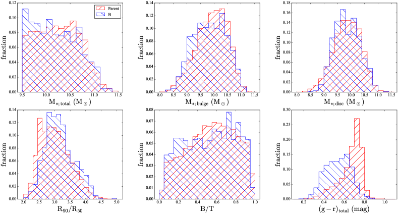
Figure 1: Normalized distributions of stellar properties for the parent sample (red) and sample B (blue).

2.5 Correlation analysis method

We use correlation coefficients to study the link between properties. We use the Pearson correlation coefficient to indicate the strength of linear correlation between two parameters. Positive and negative coefficients indicate positive and anti-correlations, respectively. The absolute value ranges from 0 to 1, and absolute values above 0.4 are considered to indicate a relatively strong correlation compared to the relation between randomly distributed parameter pairs. We also calculate the Spearman correlation coefficient as supplementary information to the Pearson correlation coefficient. It quantifies the correlation between the ranks of two parameters, so the correlation is not necessarily linear.

Because many galactic properties correlate with each other (e.g. both colour and $f_{\rm{HI}}$ are correlated with $M_{\star}$ in star-forming galaxies), there is possibility that a correlation between two parameters is caused by dependence of both parameters on a third parameter. Here we rely on two ways to identify a possible intrinsic (independent of parameter $C$) linear correlation between two parameters $A$ and $B$. In the first way, we calculate the partial correlation coefficient. The partial correlation coefficient between A and B, with a third control parameter C, is defined as $\rho_{AB,C}=\left(\rho_{AB}-\rho_{AC}\rho_{BC}\right)/\sqrt{\left(1-\rho_{AC}^{2}\right)\left(1-\rho_{BC}^{2}\right)}$, where $\rho_{AB}$ is the Pearson correlation correlation between $A$ and $B$ (similar for $\rho_{AC}$ and $\rho_{BC}$). We use two methods to justify the significance of correlations. Firstly, we calculate errors of the coefficients through bootstrapping. We resample the data with replacement for 2000 times, and thereby build 2000 new samples. We calculate the correlation coefficient for each new sample and thereby obtain a distribution of 2000 correlation coefficients. The standard deviation of the distribution is taken as the error of the correlation coefficient of the original sample. Secondly, we use the python package Pingouin (Vallat, 2018) to calculate a 95% parametric confidence interval ($\pm$2 sigma) and two-tailed non-hyopthesis p-value for each correlation coefficient. Higher absolute values of correlation coefficients (after considering the uncertainties quantified by error bars or confidence intervals) should indicate stronger correlation. We also find that all the significant correlations ($\rho>0.4$) in this study have a p-value less than 0.001, indicating that the null hypothesis of no correlations is rejected with a 0.001 significance level ($>3$ sigma confidence level), and hence these correlations are indeed significant. Some of the very weak correlations, instead, have high p-values (e.g. the partial correlation between $f_{\rm{HI,total}}$ and ${(g-r)_{\rm disc}}$ controlled by ${M_{\rm\star,total}}$, see Section 3). We don’t consider parameter uncertainties during the calculation of correlation coefficient, but in sample selection we have removed data with large error bars.

In the second way, we divide the sample into sub-samples by the control parameter $C$, and plot the median relation between $A$ and $B$ in each sub-sample. If the correlation between $A$ and $B$ is independent of $C$, we would expect the median relations of different $C$ bins to be close to each other. On the contrary, if the $A$ versus $B$ relation of different $C$ bins differ significantly from each other and even have no overlapping between the adjacent $C$ bins, then it would indicate the intrinsic correlation between $A$ and $B$ to be very weak (even if they appear to be correlated in each individual $C$ bin).

3 Results

To explore the relation between the Hi gas and the formation of discs and bulges, we study the dependence of the colours of the discs and the bulges on the Hi gas fraction. Hi is the reservoir of material for forming stars, and colour indicates the specific star formation rate (defined as $\mathrm{SFR}/M_{\star}$ the star formation rate over the mass of stars formed). A strong correlation between the colour of a stellar component and the Hi gas fraction will indicate a strong link between the formation of this stellar component and the Hi gas.

In Fig. 2, we show how the bulge and disc colour as a function of $f_{\rm{HI}}$. The sample is divided into sub-samples by stellar mass, as denoted in the top-right corner of each panel, different colours indicating different stellar mass bins. For each $M_{\star}$ divided sub-sample, we further divide it into different $f_{\rm{HI}}$ bins. We exclude bins with less than 10 galaxies to ensure statistical significance. We use the median value and its error derived through bootstrapping (large solid dots and error bars) to quantify the distribution of data points in the bin. The trend of these median values give a visual impression how strongly parameters are correlated (supplementary to the quantification with partial correlation coefficients, see Section 2.5). Replacing median values with mean values does not significantly change the overall trend. We also show the Pearson, Spearman and partial correlation coefficients in the bottom-left corner of each panel. These correlation coefficients for all the parameter pairs investigated in this paper, as well as their 1-$\sigma$ error bars, 95% confidence intervals, and p-values, are summarized in Table 2.

At first glance, there is a considerable anti-correlation between the bulge colour and $f_{\rm{HI}}$, with a Pearson correlation coefficient of $-0.49$. However, the bulge colours are nearly constant as a function of the $f_{\rm{HI}}$ in each stellar mass bin, and we only get a partial correlation coefficient of $-0.14$ between them after removing the effect of the stellar mass. This means that when the stellar masses are controlled, there is no intrinsic correlation between bulge colour and $f_{\rm{HI}}$.

On the other hand, for the disc component, there is considerable correlation between $f_{\rm{HI}}$ and colour in each stellar mass bin. The partial coefficient is $-0.34$ with the effect of the stellar mass removed. So dependencies on $M_{\star}$ could not fully explain the link between the disc colour and $f_{\rm{HI}}$.

We find that $f_{\rm{HI}}$ may be more closely related to the stellar population in the disc than that in the bulge. We perform the following tests to further check this result. We assume that all Hi is associated only with the disc but not with the bulge, and define a new parameter $f_{\rm{HI,disc}}={M_{\rm HI}}/{M_{\rm\star,disc}}$. We check this assumption in Fig. 3, which is similar as Fig. 2, except that $f_{\rm{HI}}$ is replaced by $f_{\rm{HI,disc}}$ or $f_{\rm{HI,bulge}}$. If this assumption is correct, we would find a tighter correlation of the disc colour versus $f_{\rm{HI,disc}}$, than versus $f_{\rm{HI}}$. This is indeed what we find in Fig. 3(b). Moreover when removing the effect of the disc stellar mass, the correlation is still significant with partial correlation of $-0.49$. We do a similar test with the bulge, and define a new parameter $f_{\rm{HI,bulge}}={M_{\rm HI}}/{M_{\rm\star,bulge}}$. As shown in Fig. 3(a), the partial correlation between $f_{{\rm H}{\textsc{i}},bulge}$ and bulge colour is as weak as the partial correlation between $f_{\rm{HI}}$ and the bulge colour.

Hence we find that for both discs and bulges, the colours are correlated with the stellar masses, but the former also show correlation with $f_{\rm{HI}}$ while the latter does not. It is not surprising to find such different dependences of bulges and discs on $f_{\rm{HI}}$, as bulges can be classical and be formed via mergers of other galaxies (Kauffmann et al., 1993; Baugh et al., 1996), or the infall of massive star-forming clumps at high redshift (Genzel et al., 2008; Bournaud et al., 2014; Dekel & Krumholz, 2013; Perez et al., 2013), and then have no direct relation with the current status of the Hi gas. In the following sections, we specifically select the bulges that are likely to be secularly formed and investigate their relation with the Hi gas. We also investigate how the correlation between disc colour and $f_{\rm{HI}}$ is affected by the structural properties of the disc and the bulge.

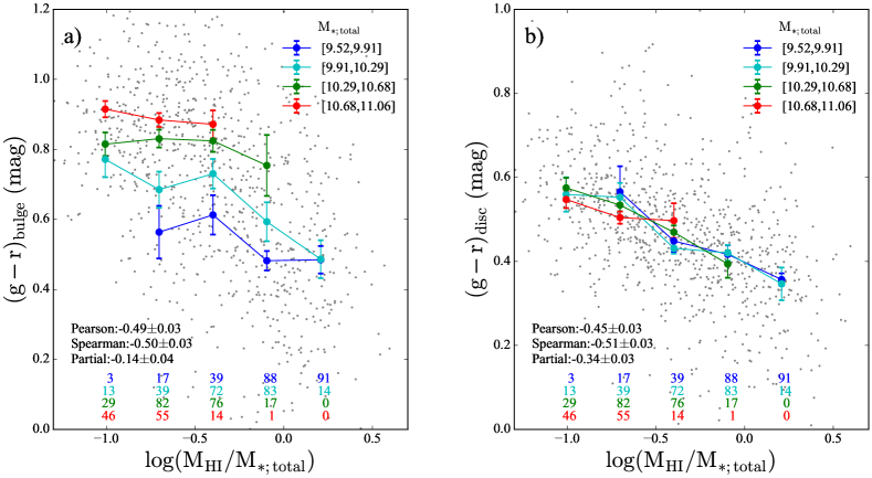
Figure 2: The dependence of bulge (left) and disc (right) colours on $f_{\rm{HI}}$. The sample is divided into sub-samples by the stellar mass, as denoted in the top-right corner of each panel. The large solid dots and error bars are the the median value and its error derived through bootstrapping. These coloured dots provide a visual impression of the strength of correlations (see Section 2.5). The number of galaxies in each sub-sample is denoted in the bottom of each panel. Pearson, Spearman and partial correlation (with the effect of the stellar mass removed) coefficients of all the data points are shown on the bottom left of each panel.

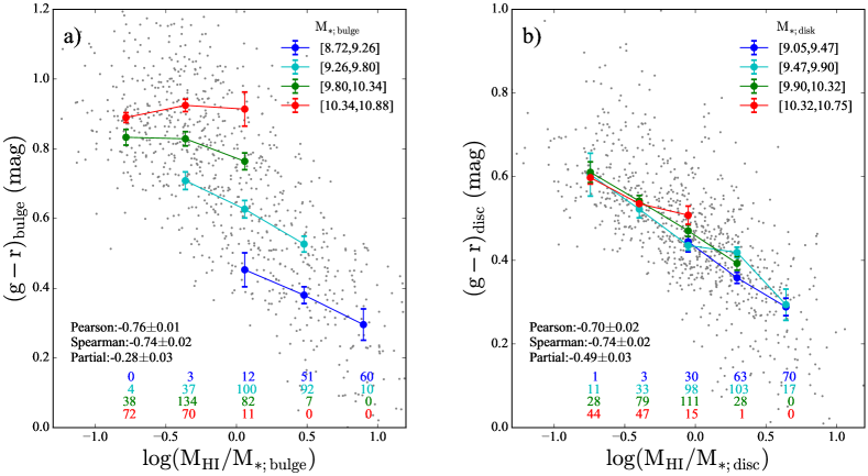
Figure 3: The dependence of bulge colours on $f_{\rm{HI,bulge}}$ (left) and disc colours on $f_{\rm{HI,disc}}$ (right) (see Sect. 3). Similar as Fig. 2, except that $f_{\rm{HI}}$ is replaced by $f_{\rm{HI,disc}}$ or $f_{\rm{HI,bulge}}$.

3.1 The bulge colour and the HI gas

We have shown that the bulge colour depends more strongly on ${M_{\rm\star,bulge}}$ than on $f_{\rm{HI}}$. We investigate whether this result holds for the secularly evolving pseudo bulges in this section. We hence plot the dependence of bulge colours on $f_{\rm{HI}}$ for different types of galaxies, as shown in Fig. 4.

Pseudo bulges are disk-like while classical bulges are not; including the classical bulges may have smeared a possible correlation between the colour of the pseudo bulge and $f_{\rm{HI}}$. So we divide the sample by bulge type, where the pseudo bulges have Sersic $n<2.5$ and the others are classical bulges (see Section 2). However, as shown in Fig. 4(a) and (b), the bulge colours depends more strongly on $M_{\star}$ than on $f_{\rm{HI,bulge}}$, for the mean ${(g-r)_{\rm bulge}}-f_{\rm{HI,bulge}}$ relations of adjacent $M_{\star}$ bins depart significantly from each other in the intercepts, e.g. the reddest ${(g-r)_{\rm bulge}}$ of the blue curve is bluer than the bluest ${(g-r)_{\rm bulge}}$ of the cyan curve.

Bars are an efficient way of driving gas inflows and secularly forming the central bulges (Wang et al., 2012), so we would expect that a correlation between the stellar population and $f_{\rm{HI}}$ may be found for the barred galaxies. But we don’t see any significant trend between the bulge colours and $f_{\rm{HI}}$ at fixed bulge stellar mass for barred galaxies (Fig. 4 (c)).

Tidal interactions are also an efficient way to drive gas inflows and enhance the central star formation (Toomre & Toomre, 1972; Keel, 1991; Struck, 1999). As described in Section 2.4, we use neighbour counts and morphological parameters to select the potentially interacting galaxies. Both parameters are found in the literature to be correlated with enhanced central SFR (Li et al., 2008; Reichard et al., 2009). When the samples are small, we show trends with fewer ${M_{\rm\star,bulge}}$ and $f_{\rm{HI,bulge}}$ bins. We find no significant correlation between the bulge colour and $f_{\rm{HI}}$ for the interacting galaxies (Fig. 4 (d,e)).

One question is whether the bulge colour could be more closely related to ${M_{\rm\star,total}}$ than to ${M_{\rm\star,bulge}}$, as galaxy evolution strongly depends on the total stellar mass (Kauffmann et al., 2003), and massive galaxies tend to have more massive and redder bulges (Peletier & Balcells, 1996; Bell & de Jong, 2000). In Fig. 5 (a), we show that the bulge colour is more strongly correlated with the bulge mass than the total stellar mass. It was hence proper to use ${M_{\rm\star,bulge}}$ as a control parameter when investigating the relation between the colour and $f_{\rm{HI}}$ of bulges.

Another possible worry is that the bulge colours used here may actually reflect the attenuation or gas phase metallicity, as colours not only depend on the stellar age, but also on these two properties (Fitzpatrick, 1999; Worthey, 1994). In Fig. 5 (b) and (c), we show that neither the metallicities nor the dust attenuations can fully explain the correlation between the bulge colours and the bulge masses. It supports the usage of colour as an indicator of the star-forming status in the bulges.

In summary, we find that for all the different sub-samples, the star formation in the (pseudo) bulges is strongly correlated with the stellar mass of the bulges, but not correlated with $f_{\rm{HI}}$ of the galaxies. We note that if we replace $f_{\rm{HI}}$ by $f_{\rm{HI,bulge}}$, the general trends in this section do not significantly change.

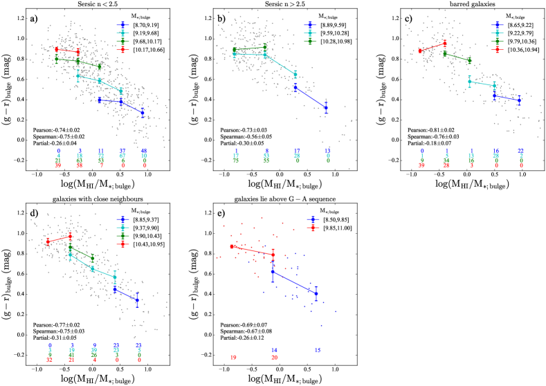
Figure 4: The dependence of bulge colours on $f_{\rm{HI}}$. Similar as the left panel of Fig. 2, but the sample is replaced by galaxies with pseudo bulges (a), galaxies with classical bulges (b), galaxies with bars (c) and galaxies experiencing galactic interactions (d,e). The sample is divided into sub-samples by the bulge mass, as denoted in the top-right corner of each panel. Same symbols and errorbars as Fig. 2.

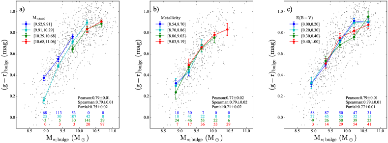
Figure 5: The dependence of ${(g-r)_{\rm bulge}}$ on the bulge mass. The sample is divided into sub-samples by the bulge mass, gas phase metallicity, or E(B-V), as denoted in the top-left corner of each panel. Same symbols and errorbars as Fig. 2.

3.2 The disc colour and the HI gas

We have shown that $f_{\rm{HI}}$ is not correlated with the bulge colour, but strongly correlated with the disc colour. This suggests that the Hi content is more closely related to the disc component than the bulge component. We therefore use $f_{\rm{HI,disc}}$ to investigate how the formation of the disc is affected by structural properties of the disc and the bulge.

It is unclear whether bulges directly play a role in the evolution of galaxies by stabilizing the discs with their centrally concentrated potential (Martig et al., 2009). So we investigate whether properties of the bulge have an influence on the relation between the disc colour and $f_{\rm{HI,disc}}$. If the bulge quenching mechanism plays a major role in reducing the star forming efficiency in our sample, we would expect to observe an on average redder ${(g-r)_{\rm disc}}$ at a fixed $f_{\rm{HI,disc}}$ for galaxies with significant bulges than for galaxies with less significant ones.

From Fig. 6, we can see that the partial correlation coefficients between ${(g-r)_{\rm disc}}$ and $f_{\rm{HI,disc}}$ are between -0.63 and -0.73 for different control parameters ($B/T$, ${M_{\rm\star,bulge}}$, $\mu_{\rm\star,bulge}$ or Sersic $n$), very close to the Pearson correlation coefficient of -0.70. It suggests that disc colours do not depend on $B/T$, ${M_{\rm\star,bulge}}$, $\mu_{\rm\star,bulge}$ or Sersic $n$. Therefore we do not find evidence for the disc colours to be affected by the existence or properties of bulges.

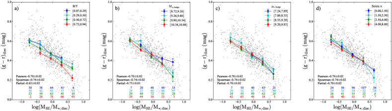
Figure 6: The dependence of disc colour on $f_{\rm{HI,disc}}$. The sample is divided into sub-samples by the $B/T$ (a), stellar masses (b), stellar surface mass densities (c) of bulges and bulge Sersic n index (d). Same symbols and errorbars as Fig. 2.

3.3 The relation between the bulge colour and the disc colour

In previous sections, we have shown that the bulge colour is largely independent of $f_{\rm{HI}}$, while the disc colour is strongly correlated with $f_{\rm{HI}}$. These results indicate that the bulge and the disc evolve in different ways, even when both are evolving (mostly) secularly at low redshift. We confirm this point in Fig. 7, that bulge colours are not correlated with disc colours in a positive way, when the bulge mass is controlled.

It is possible that the bulge and the disc differ in colours due to different characteristic sizes. So we compare their colour radial distributions. We plot median colour profiles for the bulge and disc components in each total mass bin. In Fig. 8, we can see that at a fixed radius, there is indeed a general trend for galaxies which have high ${M_{\rm\star,total}}$ to have redder colours in both the bulges and the discs than the galaxies with low ${M_{\rm\star,total}}$. However, at a fixed radius, bulge colours vary much more significantly as a function of ${M_{\rm\star,total}}$ than disc colours. When $r=0.5R_{\rm e}$, the average bulge colours increase from 0.4 to 0.9 mag when ${M_{\rm\star,total}}$ increases, but disc colours only increase from 0.4 to 0.65 mag. In a fixed ${M_{\rm\star,total}}$ bin, the average disc colours also vary much less significantly as a function of radius than bulge colours. All these results suggest a significant difference in the stellar population between the bulge and the disc.

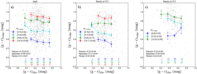
Figure 7: The dependence of bulge colour on disc colour for total, pseudo bulge ($n<2.5$) and classical bulges ($n>2.5$) respectively. Different colours indicate different bulge stellar mass bins, as denoted in the middle-left corner of each panel. Same symbols and errorbars as Fig. 2.

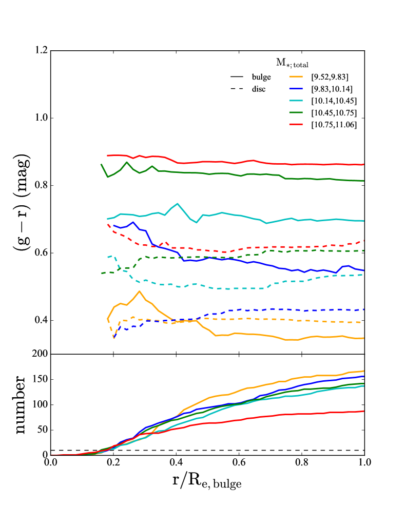
Figure 8: Top: The median colour profiles for the bulge (solid) and disc (dashed) components in different total mass bins. For each galaxy, only data points with radius larger than 0.5 times the FWHM of SDSS are used. Different colours indicate different stellar mass bins, as denoted in the top-right corner. The profile is plotted out to the effective radius of the bulge; Bottom: The number of galaxies in each radius bin. The dashed horizontal line is at a level of 10, which is the minimum number of galaxies to calculate median colour profile.

3.4 $f_{\rm{HI}}$ and the bulge/disc structures

Catinella et al. (2010) showed that $f_{\rm{HI}}$ is correlated with the stellar mass surface density but not with the concentration, hence we study how bulge or disc structures affect $f_{\rm{HI}}$ in a decomposed view.

Firstly, from Fig. 9(a), we shown that $f_{\rm{HI}}$ is independent of $B/T$, which is consistent with the finding that $f_{\rm{HI}}$ only shows a weak correlation with concentration, as $B/T$ is tightly correlated with the concentration. Hence the trend of decreasing $f_{\rm{HI}}$ with increasing $\mu_{\star}$ (Catinella et al. 2010, also panel b of Fig. 9) is unlikely caused by the increased significance of bulges, although $\mu_{\star}$ is correlated with $B/T$. Instead, we also find a correlation between $f_{\rm{HI,disc}}$ and $\mu_{\rm\star,disc}$ (panel c of Fig. 9), indicating that the disc structure itself may affect or reflect the ${\rm H}{\textsc{i}}$ content of galaxies.

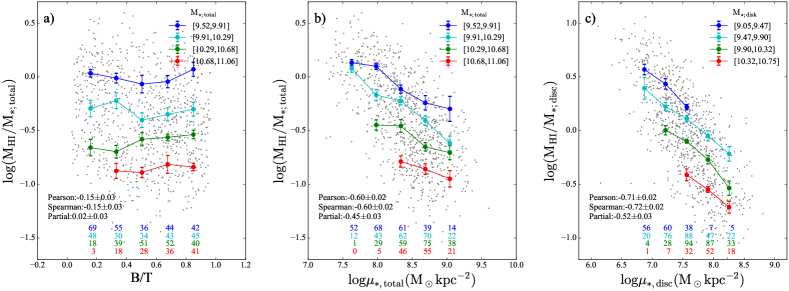
Figure 9: The dependence of $f_{\rm{HI,total}}$ on $B/T$ (a), $f_{\rm{HI,total}}$ on total surface mass density (b) and $f_{\rm{HI,disc}}$ on disk surface mass density (c). The sample is divided into sub-samples by the total stellar masses (a,b) or disc stellar masses (c). Different colours indicate different disc stellar mass bins. Same symbols and errorbars as Fig. 2.

4 Summary and discussion

In this work, we used a sample of 858 SDSS galaxies with Hi data from ALFALFA and photometric bulge-to-disc decompositions from M15 to investigate the relation between Hi content and bulge/disc properties. We found that both the disc colour and the bulge colour are strongly correlated with $f_{\rm{HI}}$, but for different reasons. The correlation between the disc colour and $f_{\rm{HI}}$ is largely independent of the disk stellar mass. The correlation between the bulge colour and $f_{\rm{HI}}$ is intrinsically weak, and is caused by both parameters depending on the stellar mass of the bulge. Consistently, the colours of the bulge and the disc are not significantly correlated when the bulge mass is controlled. These results about bulges hold when only pseudo bulges are considered. The results suggest the different ways that bulges and discs form.

In cosmological models, discs form inside-out as a result of gas accretion from the circum-galactic medium (Kauffmann, 1996; Mo et al., 1998). The strong correlation between disk colours and $f_{\rm{HI}}$ is consistent with this model. This model was supported by earlier observations that the colours of the outer regions of galaxies depend more strongly on $f_{\rm{HI}}$ than the inner regions (Wang et al., 2011). In this paper, instead of dividing galaxies into the bulge and disc dominated inner and outer regions, we directly use the colours of disc components and find a strong correlation with $f_{\rm{HI}}$, providing more direct support to the inside-out formation model than before. Moreover, we do not find evidence for the star formation in the discs to be quenched by the bulges.

It is well accepted that pseudo bulges are different from classical bulges but similar to discs. They tend to be star-forming and distribute similarly in the structural fundamental plane as discs (Martig et al., 2009; Gadotti, 2009). One may hence expect the star formation rate of pseudo bulges to be also correlated with the Hi content of galaxies. However, we find this correlation to be weak. The reason is likely that the Hi gas needs time to flow inward in order to reach the bulge. Effective inflows of gas can be driven by torques provided by bars (as a non-axisymmetric structures in galaxies), or external tidal effects (Kormendy & Kennicutt, 2004). The strength of tidal effects depend on the mass and orbit of the interacting companions (Larson, 2002), and the strength of bars depend on the length, ellipticity and mass of bars (Wang et al., 2012; Regan & Teuben, 2004). The inflow rates of Hi hence may differ significantly among galaxies which have bar or are interacting, and the correlation between the bulge colour and $f_{\rm{HI}}$ therefore may tend to have large scatter in these galaxies. Additional scatter between the colour and $f_{\rm{HI}}$ could be caused by the fact that star formation triggered by strong inflows could be episodic, due to the high central mass concentration (hence strong shearing), quick consumption of gas, and$/$or strong stellar feedback (Maciejewski et al., 2002; Sheth et al., 2005; Krumholz & Kruijssen, 2015). As a result of these complexities, the fraction of the Hi that actually reaches the bulge region is uncertain, and the formation of the pseudo bulge can be temporarily detached from the formation of the discs.

In semi-analytical models, the formation of a pseudo bulge is often empirically treated as the result of disc instabilities that emerge when a certain critical density is reached in the disc (e.g. Kauffmann et al., 2012). The critical densities are reached when significant amount of gas flows inward, and hence is not directly related to the integrated gas fractions. This empirical treatment is qualitatively consistent with the way that pseudo bulges form as indicated by the results of this paper. But more details about the formation of pseudo bulges that can be compared with or constrain the cosmological models are largely missing. These details can be quantified as the inflow rate of gas to the bulge regions and the consequent surface density distribution of cold gas in the bulge regions; also relevant are the circular velocity and velocity dispersion of the cold gas that may affect the efficiency of converting the gas to stars of the bulges. These measurements need be extracted from high-resolution images of cold gas, for statistically significant samples of galaxies, which may be available in the coming years when large HI surveys with the Square Kilometre Array and its precursor telescopes start.

We point out that our sample only includes relatively star-forming galaxies which have ALFALFA detections. The results relevant to the quenching of star formation rate (bulge quenching) could be affected by this selection effect. Also, we only investigated the relation between the HI and star formation rate (SFR), because we do not have data for the molecular gas. It is possible that the conversion between HI and H2 or between H2 and SFR could be more affected by the bulge than the less direct relation between the HI and SFR. Because the bulge-disc decomposition catalogue used in this paper was produced by a pipeline (Vikram et al., 2010), large uncertainties in the fitting could exist for individual galaxies. Our investigation is hence limited to the statistical aspect. Analysis based on deeper Hi data (the x-GASS sample Catinella et al., 2018), as well as more careful component decomposition for individual galaxies, is currently under way (Cook et al., 2019).

References

- Allen et al. (2006) Allen P. D., Driver S. P., Graham A. W., Cameron E., Liske J., de Propris R., 2006, MNRAS, 371, 2
- Andredakis & Sanders (1994) Andredakis Y. C., Sanders R. H., 1994, MNRAS, 267, 283
- Athanassoula (2005) Athanassoula E., 2005, MNRAS, 358, 1477
- Barnes et al. (2001) Barnes D. G., et al., 2001, MNRAS, 322, 486
- Baugh et al. (1996) Baugh C. M., Cole S., Frenk C. S., 1996, MNRAS, 283, 1361
- Bell & de Jong (2000) Bell E. F., de Jong R. S., 2000, MNRAS, 312, 497
- Bournaud et al. (2014) Bournaud F., et al., 2014, ApJ, 780, 57
- Carollo et al. (2007) Carollo D., et al., 2007, Nature, 450, 1020
- Catinella et al. (2010) Catinella B., et al., 2010, MNRAS, 403, 683
- Catinella et al. (2018) Catinella B., et al., 2018, MNRAS, 476, 875
- Charlot & Longhetti (2001) Charlot S., Longhetti M., 2001, MNRAS, 323, 887
- Cook et al. (2019) Cook R. H. W., Cortese L., Catinella B., Robotham A., 2019, MNRAS, 490, 4060
- Dekel & Krumholz (2013) Dekel A., Krumholz M. R., 2013, MNRAS, 432, 455
- Fabello et al. (2011) Fabello S., Catinella B., Giovanelli R., Kauffmann G., Haynes M. P., Heckman T. M., Schiminovich D., 2011, MNRAS, 411, 993
- Fisher & Drory (2010) Fisher D. B., Drory N., 2010, ApJ, 716, 942
- Fisher & Drory (2016) Fisher D. B., Drory N., 2016, Galactic Bulges, 418, 41
- Fitzpatrick (1999) Fitzpatrick E. L., 1999, The Publications of the Astronomical Society of the Pacific, 111, 63
- Gadotti (2009) Gadotti D. A., 2009, MNRAS, 393, 1531
- Genzel et al. (2008) Genzel R., et al., 2008, ApJ, 687, 59
- Giovanelli et al. (2005) Giovanelli R., et al., 2005, The Astronomical Journal, 130, 2598
- Hart et al. (2016) Hart R. E., et al., 2016, MNRAS, 461, 3663
- Häußler et al. (2013) Häußler B., et al., 2013, MNRAS, 430, 330
- Haynes et al. (2018) Haynes M. P., et al., 2018, ApJ, 861, 49
- Kauffmann (1996) Kauffmann G., 1996, MNRAS, 281, 475
- Kauffmann et al. (1993) Kauffmann G., White S. D. M., Guiderdoni B., 1993, MNRAS, 264, 201
- Kauffmann et al. (2003) Kauffmann G., et al., 2003, Monthly Notice of the Royal Astronomical Society, 341, 54
- Kauffmann et al. (2012) Kauffmann G., et al., 2012, MNRAS, 422, 997
- Keel (1991) Keel W. C., 1991, in Dynamics of Galaxies and Their Molecular Cloud Distributions: Proceedings of the 146th Symposium of the International Astronomical Union. pp 243–
- Koribalski et al. (2004) Koribalski B. S., et al., 2004, The Astronomical Journal, 128, 16
- Kormendy (1993) Kormendy J., 1993, in Galactic bulges: proceedings of the 153rd Symposium of the International Astronomical Union held in Ghent. pp 209–
- Kormendy & Kennicutt (2004) Kormendy J., Kennicutt R. C. J., 2004, Annual Review of Astronomy &Astrophysics, 42, 603
- Kormendy et al. (2010) Kormendy J., Drory N., Bender R., Cornell M. E., 2010, ApJ, 723, 54
- Krumholz & Kruijssen (2015) Krumholz M. R., Kruijssen J. M. D., 2015, MNRAS, 453, 739
- Lackner & Gunn (2012) Lackner C. N., Gunn J. E., 2012, MNRAS, 421, 2277
- Larson (2002) Larson R. B., 2002, MNRAS, 332, 155
- Li et al. (2008) Li C., Kauffmann G., Heckman T. M., Jing Y. P., White S. D. M., 2008, MNRAS, 385, 1903
- Lotz et al. (2004) Lotz J. M., Primack J., Madau P., 2004, The Astronomical Journal, 128, 163
- Maciejewski et al. (2002) Maciejewski W., Teuben P. J., Sparke L. S., Stone J. M., 2002, MNRAS, 329, 502
- Martig et al. (2009) Martig M., Bournaud F., Teyssier R., Dekel A., 2009, ApJ, 707, 250
- Masters et al. (2011) Masters K. L., et al., 2011, MNRAS, 411, 2026
- Meert et al. (2015) Meert A., Vikram V., Bernardi M., 2015, MNRAS, 446, 3943
- Meert et al. (2016) Meert A., Vikram V., Bernardi M., 2016, MNRAS, 455, 2440
- Meyer et al. (2004) Meyer M. J., et al., 2004, MNRAS, 350, 1195
- Mo et al. (1998) Mo H. J., Mao S., White S. D. M., 1998, MNRAS, 295, 319
- Peletier & Balcells (1996) Peletier R. F., Balcells M., 1996, Astronomical Journal v.111, 111, 2238
- Perez et al. (2013) Perez J., Valenzuela O., Tissera P. B., Michel-Dansac L., 2013, MNRAS, 436, 259
- Regan & Teuben (2004) Regan M. W., Teuben P. J., 2004, ApJ, 600, 595
- Reichard et al. (2009) Reichard T. A., Heckman T. M., Rudnick G., Brinchmann J., Kauffmann G., Wild V., 2009, ApJ, 691, 1005
- Roberts & Haynes (1994) Roberts M. S., Haynes M. P., 1994, ARA&A, 32, 115
- Sheth et al. (2005) Sheth K., Vogel S. N., Regan M. W., Thornley M. D., Teuben P. J., 2005, ApJ, 632, 217
- Simard et al. (2011) Simard L., Mendel J. T., Patton D. R., Ellison S. L., McConnachie A. W., 2011, ApJS, 196, 11
- Struck (1999) Struck C., 1999, Physics Reports, 321, 1
- Teimoorinia et al. (2017) Teimoorinia H., Ellison S. L., Patton D. R., 2017, MNRAS, 464, 3796
- Toomre & Toomre (1972) Toomre A., Toomre J., 1972, Astrophysical Journal, 178, 623
- Tremonti et al. (2004) Tremonti C. A., et al., 2004, ApJ, 613, 898
- Vallat (2018) Vallat R., 2018, The Journal of Open Source Software, 3, 1026
- Vikram et al. (2010) Vikram V., Wadadekar Y., Kembhavi A. K., Vijayagovindan G. V., 2010, MNRAS, 409, 1379
- Wang et al. (2011) Wang J., et al., 2011, MNRAS, 412, 1081
- Wang et al. (2012) Wang J., et al., 2012, MNRAS, 423, 3486
- Willett et al. (2013) Willett K. W., et al., 2013, MNRAS, 435, 2835
- Worthey (1994) Worthey G., 1994, ApJS, 95, 107
- Zibetti et al. (2009) Zibetti S., Charlot S., Rix H.-W., 2009, MNRAS, 400, 1181