Federated Learning with Cooperating Devices: A Consensus Approach for Massive IoT Networks

Abstract

Federated learning (FL) is emerging as a new paradigm to train machine learning models in distributed systems. Rather than sharing, and disclosing, the training dataset with the server, the model parameters (e.g., neural networks weights and biases) are optimized collectively by large populations of interconnected devices, acting as local learners. FL can be applied to power-constrained IoT devices with slow and sporadic connections. In addition, it does not need data to be exported to third parties, preserving privacy. Despite these benefits, a main limit of existing approaches is the centralized optimization which relies on a server for aggregation and fusion of local parameters; this has the drawback of a single point of failure and scaling issues for increasing network size. The paper proposes a fully distributed (or server-less) learning approach: the proposed FL algorithms leverage the cooperation of devices that perform data operations inside the network by iterating local computations and mutual interactions via consensus-based methods. The approach lays the groundwork for integration of FL within 5G and beyond networks characterized by decentralized connectivity and computing, with intelligence distributed over the end-devices. The proposed methodology is verified by experimental datasets collected inside an industrial IoT environment.

I Introduction

Beyond 5G systems are expected to leverage cross-fertilizations between wireless systems, core networking, Machine Learning (ML) and Artificial Intelligence (AI) techniques, targeting not only communication and networking tasks, but also augmented environmental perception services [1]. The combination of powerful AI tools, e.g. Deep Neural Networks (DNN), with massive usage of Internet of Things (IoT), is expected to provide advanced services [2] in several domains such as Industry 4.0 [3], Cyber-Physical Systems (CPS) [4] and smart mobility [5]. Considering this envisioned landscape, it is of paramount importance to integrate emerging deep learning breakthroughs within future generation wireless networks, characterized by arbitrary distributed connectivity patterns (e.g., mesh, cooperative, peer-to-peer, or spontaneous), along with strict constraints in terms of latency [6] (i.e., to support Ultra-Reliable Low-Latency Communications - URLLC) and battery lifetime.

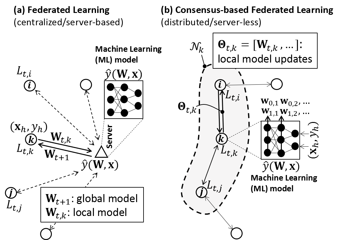
Figure 1: From left to right: a) FL based on centralized fusion of local model (or gradient) updates; b) proposed consensus-based FL with distributed fusion over an infrastructure-less network. Learning of global model parameters $\mathbf{W}$ from local data examples $(\mathbf{x}_{h},y_{h})$ is obtained by mutual cooperation between neighbors sharing the local model updates $\Theta_{t,k}$.

Recently, federated optimization, or federated learning (FL) [7][8] has emerged as a new paradigm in distributed ML setups [9]. The goal of FL systems is to train a shared global model (i.e., a Neural Network - NN) from a federation of participating devices acting as local learners under the coordination of a central server for models aggregation. As shown in Fig. 1.a, FL alternates between a local model computation at each device and a round of communication with a server. Devices, or workers, derive a set of local learning parameters from the available training data, referred to as local model. The local model $\mathbf{W}_{t,k}$ at time $t$ and device $k$ is typically obtained via back-propagation and Stochastic Gradient Descent (SGD) [10] methods using local training examples $\textrm{(}i.e.,\textrm{data }\mathbf{x}_{h},\textrm{and labels }y_{h}\textrm{)}$. The server obtains a global model by fusion of local models and then feeds back such model to the devices. Multiple rounds are repeated until convergence is reached. The objective of FL is thus to build a global model $y=\hat{y}(\mathbf{W};\mathbf{x})$ by the cooperation of a number of devices. Model is characterized by parameters $\mathbf{W}$ (i.e., NN weights and biases for each layer) for the output quantity $y$ and the observed (input) data $\mathbf{x}$. Since it decouples the ML stages from the need to send data to the server, FL provides strong privacy advantages compared to conventional centralized learning methods.

I-A Decentralized FL and related works

Next generation networks are expected to be underpinned by new forms of decentralized, infrastructure-less communication paradigms [11] enabling devices to cooperate directly over device-to-device (D2D) spontaneous connections (e.g., multihop or mesh). These networks are designed to operate - when needed - without the support of a central coordinator, or with limited support for synchronization and signalling. They are typically deployed in mission-critical control applications where edge nodes cannot rely on a remote unit for fast feedback and have to manage part of the computing tasks locally [12], cooperating with neighbors to self disclose the information. Typical examples are low-latency safety-related services for vehicular [13] or industrial [14] applications. Considering these trends, research activities are now focusing on fully decentralized (i.e., server-less) learning approaches. Optimization of the model running on the devices with privacy constraints is also critical [16] for human-related applications.

To the authors knowledge, few attempts have been made to address the problem of decentralized FL. In [17][18], a gossip protocol is adopted for ML systems. Through sum-weight gossip, local models are propagated over a peer-to-peer network. However, in FL over D2D networks, gossip-based methods cannot be fully used because of medium access control (MAC) and half-duplex constraints, which are ignored in these early approaches. More recently, [19] considers an application of distributed learning for medical data centers where several servers collaborate to learn a common model over a fully connected network. However, network scalability/connectivity issues are not considered at all. In [20], a segmented gossip aggregation is proposed. The global model is split into non overlapping subsets and local learners aggregate the segmentation sets from other learners. Having split the model, by introducing ad-hoc subsets and segment management tasks, the approach is extremely application-dependent and not suitable for more general ML contexts. Finally, [21][22] propose a peer-to-peer Bayesian-like approach to iteratively estimate the posterior model distribution. Focus is on convergence speed and load balancing, yet simulations are limited to a few nodes, and the proposed method cannot be easily generalized to NN systems trained by incremental gradient (i.e., SGD) or momentum based methods.

I-B Contributions

This paper proposes the application of FL principles to massively dense and fully decentralized networks that do not rely upon a central server coordinating the learning process. As shown in Fig. 1.b, the proposed FL algorithms leverage the mutual cooperation of devices that perform data operations inside the network (in-network) via consensus-based methods [23]. Devices independently perform training steps on their local dataset (batches) based on a local objective function, by using SGD and the fused models received from the neighbors. Next, similarly to gossip [17], devices forward the model updates to their one-hop neighborhood for a new consensus step. Unlike the methods in [17]-[22], the proposed approach is general enough to be seamlessly applied to any NN model trained by SGD or momentum methods. In addition, in this paper we investigate the scalability problem for varying NN model layer size, considering large and dense D2D networks with different connectivity graphs. These topics are discussed, for the first time, by focusing on an experimental Industrial IoT (IIoT) setting.

The paper contributions are summarized in the following:

• the federated averaging algorithm [9][15] is revisited to allow local learners to implement consensus techniques by exchanging local model updates: consensus also extends existing gossip approaches;

• a novel class of FL algorithms based on the iteratively exchange of both model updates and gradients is proposed to improve convergence and minimize the number of communication rounds, in exchange for a more intensive use of D2D links and local computing;

• all presented algorithms are validated over large scale massive networks with intermittent, sporadic or varying connectivity, focusing in particular on an experimental IIoT setup, and considering both complexity, convergence speed, communication overhead, and average execution time on embedded devices.

The paper is organized as follows. Sect. II reviews the FL problem. Sect. III proposes two consensus-based algorithms for decentralized FL. Validation of the proposed methods is first addressed in Sect. IV on a simple network and scenario. Then, in Sect. V the validation is extended to a large scale setup by focusing on a real-world problem in the IIoT domain. Finally, Sect. VI draws some conclusions and proposes future investigations.

II FL for model optimization

The FL approach defines an incremental algorithm for model optimization over a large population of devices. It belongs to the family of incremental gradient algorithms [26][29] but, unlike these setups, optimization typically focuses on non-convex objectives that are commonly found in NN problems. The goal is to learn a global model $\hat{y}(\mathbf{W};\mathbf{x})$ for inference problems (i.e., classification or regression applications) that transforms the input observation vector $\mathbf{x}$ into the outputs $\hat{y}\in\left\{y_{c}\right\}_{c=1}^{C}$, with model parameters embodied in the matrix $\mathbf{W}$ while $C$ is the output size. Observations, or input data, are stored across $K$ devices connected with a central server that coordinates the learning process. A common, and practical, assumption is that the number of participating devices $K$ is large ($K\gg 1$) and they have intermittent connectivity with the server. The cost of communication is also much higher than local computation, in terms of capacity, latency and energy consumption [25]. In this paper, we will focus specifically on NN models. Therefore, considering a NN of $Q\geq 1$ layers, the model iteratively computes a non-linear function $f(\cdot)$ of a weighted sum of the input values, namely

$$\hat{y}(\mathbf{W};\mathbf{x})=f_{Q}\left(\mathbf{w}_{0,Q}^{\mathrm{T}}\mathbf{h}_{Q-1}+\mathbf{w}_{1,Q}\right)$$ (1)

with $\mathbf{h}_{q}=f_{q}\left(\mathbf{w}_{0,q}^{\mathrm{T}}\mathbf{h}_{q-1}+\mathbf{w}_{1,q}\right)$, $q=1,...,Q-1$, being the hidden layers and $\mathbf{h}_{0}=\mathbf{x}$ the input vector. The matrix

$$\mathbf{W}=\left[\mathbf{w}_{0,1}^{\mathrm{T}},\mathbf{w}_{1,1},...,\mathbf{w}_{0,Q}^{\mathrm{T}},\mathbf{w}_{1,Q}\right]$$ (2)

collects all the parameters of the model, namely the weights $\mathbf{w}_{0,q}\in\mathbb{R}^{d_{1}\times d_{2}}$ and the biases $\mathbf{w}_{1,\mathit{q}}\in\mathbb{R}^{d_{2}\times 1}$ for each defined layer, with $d_{1}$ and $d_{2}$ the corresponding input and output layer dimensions, respectively. FL applies independently to each layer of the network. Therefore, in what follows, optimization focuses on one layer $q$ and the matrix (2) reduces to $\mathbf{W=\left[\text{$\mathbf{w}_{0,q}^{\mathrm{T}}$,$\mathbf{w}_{1,q}$}\right]}$. The parameters of the convolutional layers, namely input, output and kernel dimensions, can be easily reshaped to conform with the above general representation.

In FL it is commonly assumed [7][8] that a large database of examples is (unevenly) partitioned among the $K$ devices, under non Identical Independent Distribution (non-IID) assumptions. Examples are thus organized as the tuples $(\mathbf{x}_{h},y_{h})$, $h=1,...,E$ where $\mathbf{x}_{h}$ represents the data, while $y_{h}$ are the desired model outputs $\hat{y}$. The set of examples, or training data, available at device $k$ is $\mathcal{E}_{k}$, where $E_{k}=\left|\mathcal{E}_{k}\right|\ll E$ is the size of the k-th dataset under the non-IID assumption. The training data on a given device is thus not representative of the full population distribution. In practical setups (see Sect. V), data is collected individually by the devices based on their local/partial observations of the given phenomenon.

Unlike incremental gradient algorithms [30][31], FL of model $\mathbf{W}$ is applicable to any finite-sum objective $L(\mathbf{W})$ of the general form

$$\underset{\mathbf{W}}{\mathrm{min}}\thinspace L(\mathbf{W})=\underset{\mathbf{W}}{\mathrm{min}}\underset{L(\mathbf{W})}{\underbrace{\sum_{k=1}^{K}\frac{E_{k}}{E}\times L_{k}(\mathbf{W})},}$$ (3)

where $L_{k}(\mathbf{W})$ is the loss, or cost, associated with the $k$-th device

$$L_{k}(\mathbf{W})=\frac{1}{E_{k}}\sum_{h=1}^{E_{k}}\ell(\mathbf{x}_{h},y_{h};\mathbf{W})$$ (4)

and $\ell(\mathbf{x}_{h},y_{h};\mathbf{W})$ is the loss of the predicted model over the $E_{k}$ examples $(\mathbf{x}_{h},y_{h})$ observed by the device $k$, assuming model parameters $\mathbf{W}$ to hold.

In conventional centralized ML (i.e., learning without federation), used here as benchmark, the server collects all local training data from the devices and obtains the optimization of model parameters by applying an incremental gradient method over a number of batches from the training dataset. For iteration $t$, the model parameters are thus updated by the server according to

$$\mathbf{W}_{t+1}=\mathbf{W}_{t}-\mu_{s}\times\nabla L(\mathbf{W}_{t}),$$ (5)

where $\mu_{s}$ is the SGD step size and $\nabla L(\mathbf{W}_{t})=\nabla_{\mathbf{W}_{t}}\left[L(\mathbf{W}_{t})\right]$ the gradient of the loss in (3) over the assigned batches and w.r.t. the model $\mathbf{W}_{t}$. Backpropagation is used here for gradients computation. The model estimate at convergence is denoted as $\mathbf{W}_{\infty}=\lim_{t\rightarrow\infty}\mathbf{W}_{t}$.

Rather than sharing the training data with the server, in FL the model parameters $\mathbf{W}$ are optimized collectively by interconnected devices, acting as local learners. On each round $t$ of communication, the server distributes the current global model $\mathbf{W}_{t}$ to a subset $\mathcal{S}_{t}$ of $n_{t}$ devices. The devices independently update the model $\mathbf{W}_{t}$ using the gradients (SGD) from local training data as

$$\mathbf{W}_{t+1,k}=\mathbf{W}_{t}-\mu\times\nabla L_{t,k}(\mathbf{W}_{t}),$$ (6)

where $\nabla L_{t,k}(\mathbf{W}_{t})=\nabla_{\mathbf{W}_{t}}\left[L_{t,k}(\mathbf{W}_{t})\right]$ represents the gradient of the loss (4) observed by the $k$-th device and w.r.t. the model $\mathbf{W}_{t}$. Updates $\nabla L_{t,k}$ (6), or local models $\mathbf{W}_{t+1,k}$, are sent back to the server, after quantization, anonymization [7] and compression stages, modelled here by the operator $\mathcal{P}_{\Theta}$. A global model update is obtained by the server through aggregation according to

$$\mathbf{W}_{t+1}=\mathbf{W}_{t}-\mu_{s}\frac{1}{n_{t}}\sum_{k=1}^{n_{t}}\frac{E_{k}}{E}\mathcal{P}_{\Theta}\left[\nabla L_{t,k}(\mathbf{W}_{t})\right].$$ (7)

Convergence towards the centralized approach (5) is achieved if $\lim_{t\rightarrow\infty}\mathbf{W}_{t}=\mathbf{W}_{\infty}$. Notice that the learning rate $\mu_{s}$ is typically kept smaller [9] compared with centralized learning (5) on large datasets. Aggregation model (7) is referred to as Federated Averaging (FA) [7][15]. As far as convergence is concerned, for strongly convex objective $L(\mathbf{W})$ and generic local solvers, the general upper bound on global iteration number $N_{I}$ is given in [24] and relates both to global ($\gamma_{G}$) and local ($\gamma_{L}$) accuracy according to the equation $N_{I}=\mathcal{O\left(\log\left[\mathrm{1/\left(1-\gamma_{G}\right)}\right]\mathrm{/\gamma_{L}}\right)}$.

III A consensus-based approach to in-network FL

The approaches proposed in this section allow the devices to learn the model parameters, solution of (3), by relying solely on local cooperation with neighbors, and local in-network (as opposed to centralized) processing. The interaction topology of the network is modelled as a directed graph $\mathcal{G}=(\mathcal{V},\xi)$ with the set of nodes $\mathcal{V}=\left\{1,2,...,K\right\}$ and edges (links) $\xi$. As depicted in Fig. 1, the $K$ distributed devices are connected through a decentralized communication architecture based on D2D communications. The neighbor set of device $k$ is denoted as $\mathcal{N}_{k}=\left\{i\in V:(i,k)\in\xi\right\}$, with cardinality $\left|\mathcal{N}_{k}\right|$. Notice that we include node $k$ in the set $\mathcal{N}_{k}$, while $\mathcal{N}_{\bar{k}}=\mathcal{N}_{k}\backslash\left\{k\right\}$ does not. As introduced in the previous section, each device has a database $\mathcal{E}_{k}$ of examples $(\mathbf{x}_{h},y_{h})$ that are used to train a local NN model $\mathbf{W}_{t,k}$ at some time $t$ (epoch). The model maps input features $\mathbf{x}$ into outputs $\hat{y}(\mathbf{W}_{t,k};\mathbf{x})$ as in (1). A cost function, generally non-convex, as $L_{k}(\mathbf{W}_{t,k})$ in (4), is used to optimize the weights $\mathbf{W}_{t,k}$ of the local model.

The proposed FL approaches exploit both adaptive diffusion [31] and consensus tools [23][27] to optimally leverage the (possibly large) population of federated devices that cooperate for the distributed estimation of the global model $\mathbf{W}$, while retaining the trained data. Convergence is thus obtained if $\forall k$ it is $\lim_{t\rightarrow\infty}\mathbf{W}_{t,k}=\mathbf{W}_{\infty}$. Distributed in-network model optimization must satisfy convergence time constraints, as well as minimize the number of communication rounds. In what follows, we propose two strategies that differ in the way the model updates $\mathbf{W}_{t,k}$ and gradients $\nabla L_{t,k}$ are computed and updated.

Algorithm 1 Consensus-based Federated Averaging

1:procedure CFA($\mathcal{N}_{\bar{k}},\epsilon_{t},\alpha_{t,i}$)

2:     initialize $\mathbf{W}_{0,k}$ $\leftarrow$ device $k$

3:     for each round $t=1,2,...$ do$\triangleright$ Main loop

4:         $\mathbf{receive}$$\left\{\mathbf{W}_{t,i}\right\}_{i\in\mathcal{N}_{\bar{k}}}$$\triangleright$ RX from neighbors

5:         $\boldsymbol{\psi}_{t,k}\leftarrow\mathbf{W}_{t,k}$

6:         for all devices $i\in\mathcal{N}_{\bar{k}}$ do

7:              $\boldsymbol{\psi}_{t,k}\leftarrow\boldsymbol{\psi}_{t,k}+\epsilon_{t}\alpha_{t,i}\left(\mathbf{W}_{t,i}-\mathbf{W}_{t,k}\right)$

8:         end for

9:         $\mathbf{W}_{t+1,k}=\mathrm{\text{ModelUpdate}}(\mathit{\boldsymbol{\psi}_{t,k}})$

10:         $\mathbf{send}$($\mathbf{W}_{t+1,k}$)$\triangleright$ TX to neighbors

11:     end for

12:end procedure

13:procedure ModelUpdate($\mathit{\boldsymbol{\psi}_{t,k}}$)$\triangleright$ Local SGD

14:     $\mathcal{B}\leftarrow$ mini-batches of size $B$

15:     for batch $b\in\mathcal{B}$ do$\triangleright$ Local model update

16:         $\boldsymbol{\psi}_{t,k}\leftarrow\mathit{\boldsymbol{\psi}_{t,k}}-\mu_{t}\nabla L_{t,k}(\boldsymbol{\psi}_{t,k})$

17:     end for

18:     $\mathbf{W}_{t,k}\leftarrow\boldsymbol{\psi}_{t,k}$

19:     return($\mathbf{W}_{t,k}$)

20:end procedure

III-A Consensus based Federated Averaging (CFA)

The first strategy extends the centralized FA and it is described in the pseudocode fragment of Algorithm 1. It is referred to as Consensus-based Federated Averaging (CFA).

After initialization of $\mathbf{W}_{0,k}$ at time $t=0$, on each communication round $t>0$, device $k$ sends its model updates $\mathbf{W}_{t,k}$ (once per round) and receives weights from neighbors $\mathbf{W}_{t,i}$, $i\in\mathcal{N}_{\bar{k}}$. Based on received data, the device updates its model $\mathbf{W}_{t,k}$ sequentially to obtain the aggregated model

$$\boldsymbol{\psi}_{t,k}=\mathbf{W}_{t,k}+\epsilon_{t}\sum_{i\in\mathcal{N}_{\bar{k}}}\alpha_{k,i}\left(\mathbf{W}_{t,i}-\mathbf{W}_{t,k}\right),$$ (8)

where $\epsilon_{t}$ is the consensus step-size and $\alpha_{k,i}$, $i\in\mathcal{N}_{\bar{k}}$, are the mixing weights for the models. Next, gradient update is performed using the aggregated model $\boldsymbol{\psi}_{t,k}$ as

$$\mathbf{W}_{t+1,k}=\boldsymbol{\psi}_{t,k}-\mu_{t}\nabla L_{t,k}(\boldsymbol{\psi}_{t,k}),$$ (9)

by running SGD over a number of mini-batches of size $B<E_{k}$. Model aggregation (8) is similar to the sum-weight gossip protocol [17, 18], when setting $\epsilon_{t}=1$. However, mixing weights $\alpha_{k,i}$ are used here to combine model innovations, $\left\{\mathbf{W}_{t,i}-\mathbf{W}_{t,k}\right\}$, $i\in\mathcal{N}_{\bar{k}}$. In addition, the step-size $\epsilon_{t}$ controls the consensus stability.

Inspired by FA approaches (Sect. II), the mixing weights $\alpha_{k,i}$ are chosen as

$$\alpha_{k,i}=\frac{E_{i}}{\sum_{i\in\mathcal{N}_{\bar{k}}}E_{i}}.$$ (10)

Other choices are based on weighted consensus strategies [23], where the mixing weights $\alpha_{k,i}$ are adapted on each epoch $t$ based on current validation accuracy or loss metrics. The consensus step-size $\epsilon_{t}$ can be chosen as $\epsilon_{t}\in\left(0,1/\Delta\right),$ where $\Delta=\max_{k}\left(\sum_{i\in\mathcal{N}_{\bar{k}}}\alpha_{k,i}\right)$, namely the maximum degree of the graph $\mathcal{G}$ [28] that models the interaction topology of the network. Notice that the graph $\mathcal{G}$ has adjacency matrix $\mathit{\mathbf{A}}=[a_{k,i}]$ where $a_{k,i}=\alpha_{k,i}$ iff $i\in\mathcal{N}_{\bar{k}}$ and $a_{k,i}=0$ otherwise. Beside consensus step-size, it is additionally assumed that the SGD step-size $\mu_{t}$ is optimized for convergence: namely, the objective function value $L_{t,k}$ is decreasing with each iteration of gradient descent, or after some threshold. Convergence is further analyzed in Sect. V with experimental data.

By defining as $\Theta_{t,k}$ the set of parameters to be exchanged among neighbors, CFA requires the iterative exchange of model updates $\mathbf{W}_{t,i},$ $\forall i\in\mathcal{N}_{k}$, therefore

$$\Theta_{t,k}:=\left[\mathbf{W}_{t,k}\right].$$ (11)

III-B Consensus based Federated Averaging with Gradients Exchange (CFA-GE)

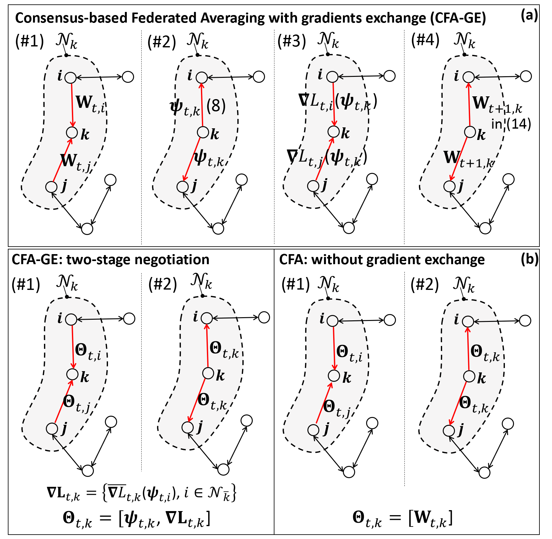
Figure 2: From top to bottom: a) CFA-GE; b) CFA-GE with two-stage negotiation and implementation (left) compared against CFA w/o gradient exchange (right).

The second strategy proposes the joint exchange of local gradients and model updates by following the four-stage iterative procedure illustrated in the Fig. 2.a for epoch $t$. The new algorithm is referred to as Consensus-based Federated Averaging with Gradients Exchange (CFA-GE). The first stage (step #1) is similar to CFA and obtains $\boldsymbol{\psi}_{t,k}$ by consensus-based model aggregation in (8). Before using $\boldsymbol{\psi}_{t,k}$ for the local model update, it is fed back to the same neighbors (“negotiation” stage in step #2 of Fig. 2.b). Model $\boldsymbol{\psi}_{t,k}$ is then used by the neighbors to compute the gradients

$$\nabla L_{t,i}(\boldsymbol{\psi}_{t,k}),\>\forall i\in\mathcal{N}_{\bar{k}}$$ (12)

using their local data. Notice that all gradients are computed over a single batch (or mini-batch) of local data, while the chosen batch/mini-batch can change on consecutive communication rounds. Gradients are sent back to the device $k$ in step #3. Compared with CFA, this step allows every device to exploit additional gradients using neighbor data, and makes the learning much faster. On the device $k$, the local model is thus updated using the received gradients (12) according to

$$\widetilde{\boldsymbol{\psi}}_{t,k}=\boldsymbol{\psi}_{t,k}-\mu_{t}\sum_{i\in\mathcal{N}_{\bar{k}}}\beta_{k,i}\mathcal{P}_{\Theta}\left[\nabla L_{t,i}(\boldsymbol{\psi}_{t,k})\right],$$ (13)

where $\beta_{k,i}$ are the mixing weights for the gradients. Finally, as done for CFA in (9), the gradient update is performed using now the aggregated model $\widetilde{\boldsymbol{\psi}}_{t,k}$ (13) and local data mini-batches

$$\mathbf{W}_{t+1,k}=\widetilde{\boldsymbol{\psi}}_{t,k}-\mu_{t}\nabla L_{t,k}(\widetilde{\boldsymbol{\psi}}_{t,k}).$$ (14)

To summarize, for each device $k$, CFA-GE combines the gradients $\nabla L_{t,k}(\boldsymbol{\psi}_{t,k})$ computed over the local data with the gradients $\nabla L_{t,i}(\boldsymbol{\psi}_{t,k})$, $i\in\mathcal{N}_{\bar{k}}$ obtained by the neighbors over their batches. The negotiation stage (13)-(14) is similar to the diffusion strategy proposed in [30][31]. In particular, we aggregate the model first (8), then we run one gradient descent round using the received gradients (13), and finally, a number of SGD rounds (14) using local mini-batches. As revealed in Sect. V, optimization of the mixing weights $\beta_{k,i}$ for the gradients is critical for convergence. Considering that the gradients in (12), obtained from neighbors, are computed over a single batch of data, as opposed to local data mini-batches, a reasonable choice is $\beta_{k,i}>1$, $\forall$$i\in\mathcal{N}_{\bar{k}}$. This aspect is further discussed in Sect. V.

Algorithm 2 CFA with gradients exchange

1:procedure CFA-GE($\mathcal{N}_{\bar{k}},\epsilon_{t},\alpha_{t,i},\beta_{t,i}$)

2:     initialize $\mathbf{W}_{0,k},\boldsymbol{\psi}_{1,k},\nabla L_{1,k}(\boldsymbol{\psi}_{0,k})$

3:     for each round $t=2,...$ do$\triangleright$ Main loop

4:         $\mathbf{receive}$$\left\{\boldsymbol{\psi}_{t,i},\overline{\nabla L}_{t,i}(\boldsymbol{\psi}_{t-1,k})\right\}_{i\in\mathcal{N}_{\bar{k}}}$$\triangleright$ RX

5:         $\boldsymbol{\psi}_{t,k}\leftarrow\mathbf{W}_{t,k}$

6:         for all devices $i\in\mathcal{N}_{\bar{k}}$ do

7:              $\boldsymbol{\psi}_{t,k}\leftarrow\boldsymbol{\psi}_{t,k}+\epsilon_{t}\alpha_{t,i}\left(\boldsymbol{\psi}_{t,i}-\mathbf{W}_{t,k}\right)$

8:              $\mathbf{compute}$ $\nabla L_{t+1,k}(\boldsymbol{\psi}_{t,i})$$\triangleright$ gradients

9:              $\overline{\nabla L}_{t+1,k}\leftarrow$ in $(\ref{eq:grad_moving})$$\triangleright$ MEWMA update

10:         end for

11:         $\boldsymbol{\widetilde{\psi}}_{t,k}\leftarrow\boldsymbol{\psi}_{t,k}$

12:         for all devices $i\in\mathcal{N}_{\bar{k}}$ do

13:              $\boldsymbol{\widetilde{\psi}}_{t,k}\negmedspace\leftarrow\negmedspace\boldsymbol{\widetilde{\psi}}_{t,k}\negthinspace-\negthinspace\mu_{t}\beta_{t,i}\overline{\nabla L}_{t,i}(\boldsymbol{\psi}_{t-1,k})$

14:         end for

15:         $\mathbf{W}_{t+1,k}\leftarrow\mathrm{ModelUpdate}\mathit{(\boldsymbol{\widetilde{\psi}}_{t,k})}$

16:         $\boldsymbol{\psi}_{t+1,k}\leftarrow\boldsymbol{\psi}_{t,k}$

17:         $\nabla\mathbf{L}_{t+1,k}:=\left\{\overline{\nabla L}_{t+1,k},\text{}\forall i\in\mathcal{N}_{\bar{k}}\right\}.$

18:         $\mathbf{send}$($\boldsymbol{\psi}_{t+1,k},\nabla\mathbf{L}_{t+1,k}$)$\triangleright$ TX to neighbors

19:     end for

20:end procedure

III-C Two-stage negotiation and implementation aspects

Unlike CFA, CFA-GE requires a larger use of the bandwidth and more communication rounds for the synchronous exchange of the gradients. More specifically, it requires a more intensive use of the D2D wireless links for sharing models first during the negotiations (step #2) and then forwarding gradients (step #3). In addition, each device should wait for neighbor gradients before applying any model update. Here, the proposed implementation simplifies the negotiation procedure to improve convergence time (and latency). In particular, it resorts to a two-stage scheme, while, likewise CFA, each device can perform the updates without waiting for a reply from neighbors. Pseudocode is highlighted in Algorithm 2. Communication rounds vs. epoch $t$ for CFA-GE are detailed in Fig. 2.b and compared with CFA. Considering the device $k$, with straightforward generalization, the following parameters are exchanged with neighbors at epoch $t$ as

$$\Theta_{t,k}:=\left[\boldsymbol{\psi}_{t,k},\nabla\mathbf{L}_{t,k}\right],$$ (15)

namely the model updates (aggregations) $\boldsymbol{\psi}_{t,k}$ and the gradients $\nabla\mathbf{L}_{t,k}$, organized as

$$\nabla\mathbf{L}_{t,k}:=\left\{\overline{\nabla L}_{t,k}(\boldsymbol{\psi}_{t-1,i}),\text{}\forall i\in\mathcal{N}_{\bar{k}}\right\}.$$ (16)

In the proposed two stage implementation, the negotiation step (step #2 in Fig. 2.a) is not implemented as it requires a synchronous model sharing. Therefore, $\forall i\in\mathcal{N}_{\bar{k}}$ the model aggregations $\boldsymbol{\psi}_{t,i}$ are not available by device $k$ at epoch $t$, or, equivalently, the device $k$ does not wait for such information from the neighbors. The gradients $\nabla L_{t,k}(\boldsymbol{\psi}_{t,i})$ are now predicted as $\overline{\nabla L}_{t,k}(\boldsymbol{\psi}_{t-1,i})$ using the past (outdated) models $\boldsymbol{\psi}_{t-1,i}$,$\boldsymbol{\psi}_{t-2,i},...$ from the neighbors. In line with momentum based techniques (see [32] and also Appendix B), for the predictions $\overline{\nabla L}_{t,k}$ we use a multivariate exponentially weighted moving average (MEWMA) of the past gradients

$$\overline{\nabla L}_{t,k}(\boldsymbol{\psi}_{t-1,i})=\varrho\nabla L_{t,k}(\boldsymbol{\psi}_{t-1,i})+(1-\varrho)\overline{\nabla L}_{t-1,k}$$ (17)

ruled by the hyper-parameter $0<\varrho\leq 1$. Setting $\varrho=1$, the gradient is estimated using the last available model ($\boldsymbol{\psi}_{t-1,i}$): $\overline{\nabla L}_{t,k}(\boldsymbol{\psi}_{t-1,i})=\nabla L_{t,k}(\boldsymbol{\psi}_{t-1,i})$. A smaller value $\varrho<1$ introduces a memory $(1-\varrho)\overline{\nabla L}_{t-1,k}$ with $\overline{\nabla L}_{t-1,k}=\overline{\nabla L}_{t-1,k}(\boldsymbol{\psi}_{t-2,i},...)$ depending on the past models $\boldsymbol{\psi}_{t-2,i},...,$. This is shown, in Sect. V, to be beneficial on real data.

Assuming that the device $k$ is able to correctly receive and decode the messages from the neighbors $\Theta_{t,i}=\left[\boldsymbol{\psi}_{t,i},\nabla\mathbf{L}_{t,i}\right]$, $\forall i\in\mathcal{N}_{\bar{k}}$ at epoch $t$, the model aggregation step changes from (8) to

$$\boldsymbol{\psi}_{t,k}=\mathbf{W}_{t,k}+\epsilon_{t}\sum_{i\in\mathcal{N}_{\bar{k}}}\alpha_{k,i}\left(\boldsymbol{\psi}_{t,i}-\mathbf{W}_{t,k}\right),$$ (18)

while the model update step using the received gradients is now

$$\widetilde{\boldsymbol{\psi}}_{t,k}=\boldsymbol{\psi}_{t,k}-\mu_{t}\sum_{i\in\mathcal{N}_{\bar{k}}}\beta_{k,i}\mathcal{P}_{\Theta}\left[\overline{\nabla L}_{t,i}(\boldsymbol{\psi}_{t-1,k})\right]$$ (19)

and replaces (13). Finally, a gradient update on local data is done as in (14). Notice that Algorithm 2 implements (19) by running one gradient descent round per received gradient (lines $12$-$14$) to allow for asynchronous updates. In the Appendix B, we discuss the application of CFA and CFA-GE to advanced SGD strategies designed to leverage momentum information [10][32].

III-D Communication overhead and complexity analysis

With respect to FA, the proposed decentralized algorithms take some load off of the server, at the cost of additional in-network operations and increased D2D communication overhead. Overhead is quantified here for both CFA and CFA-GE in terms of the size of the parameters $\Theta_{t,k}$ that need to be exchanged among neighbors. CFA extends FA and, similarly, requires each node to exchange only local model updates at most once per round. The overhead, or the size of $\Theta_{t,k}$, thus corresponds to the model size (11). For a generic DNN model of $Q$ layers, the model $\mathbf{W}_{t,k}$ size can be approximated in the order of $\mathcal{O}(d_{1}d_{2}Q)\ll E$. This is several order of magnitude lower than the size of the input training data, in typical ML and deep ML problems. As in (15), CFA-GE requires the exchange of local model aggregations $\boldsymbol{\psi}_{t,k}$ and one gradient $\overline{\nabla L}_{t,k}(\boldsymbol{\psi}_{t-1,i})$ per neighbor, $\forall i\in\mathcal{N}_{\bar{k}}$. Overhead now scales with $\mathcal{O}(d_{1}d_{2}Q\left|\mathcal{N}_{k}\right|)$, where $\left|\mathcal{N}_{k}\right|=\left|\mathcal{N}_{\bar{k}}\right|+1$. This is still considerably lower than the training dataset size, provided that the number of participating neighbors is limited. In the examples of Sect. V, we show that $\left|\mathcal{N}_{\bar{k}}\right|=2$ neighbors are sufficient, in practice, to achieve convergence: notice that the number of active neighbors is also typically small to avoid traffic issues [37]. Finally, quantization $\mathcal{P}_{\Theta}\left[\cdot\right]$ of the parameters can be also applied to limit the transmission payload, with the side effect to improve also global model generalization [38].

Besides overhead, CFA and CFA-GE computational complexity scales with the global model size and it is ruled by the number of local SGD rounds. However, unlike FA, model aggregations and local SGD are both implemented on the device. With respect to CFA, CFA-GE computes up to $\left|\mathcal{N}_{\bar{k}}\right|$ additional gradients $\overline{\nabla L}_{t,k}(\boldsymbol{\psi}_{t-1,i})$ using neighbor models $\boldsymbol{\psi}_{t-1,i}$ and up to $\left|\mathcal{N}_{\bar{k}}\right|$ additional gradient descent rounds (19) for local model update using the neighbor gradients. A quantitative evaluation of the overhead and the execution time of local computations is proposed in Sect. V by comparing FA, CFA and CFA-GE using real data and low-power System on Chip (SoC) devices.

Considering now networking aspects, the cost of a D2D communication is much lower than the cost of a server connection, typically long-range. D2D links cover shorter ranges and require lower transmit power: communication cost is thus ruled by the energy spent during receiving operations (radio wake-up, synchronization, decoding). Besides, in large-scale and massive IIoT networks, sending model updates to the server, as done in conventional FA, might need several D2D communication rounds as relaying information via neighbor devices. D2D communications can serve as an underlay to the infrastructure (server) network and can thus exploit the same radio resources. Such two-tier networks are a key concept in next generation IoT and 5G [39] scenarios.

Finally, optimal trading between in-network and server-side operations is also possible by alternating rounds of FA with rounds of in-network consensus (CFA or CFA-GE). This corresponds to a real-world scenario where communication with the server is available, but intermittent, sporadic, unreliable or too costly. During initialization, i.e. at time $t=t_{0}$, devices might use the last available global model received from the server, $\mathbf{W}_{t_{0},k}=\mathbf{W}_{N_{s}}$, after $N_{s}$ communication rounds of the previous FA phase, and obtain a local update via SGD: $\mathbf{W}_{t+1,k}=\mathbf{W}_{N_{s}}-\mu_{t}\nabla L_{t,k}(\mathbf{W}_{N_{s}})$. This is fed-back to neighbors to start CFA or CFA-GE iterations.

IV Consensus-based FL: an introductory example

In this section, we give an introductory example of consensus-based FL approaches comparing their performance to conventional FL methods. We resort here to a network of $K=4$ wireless devices communicating via multihop as depicted in Fig. 3 without any central coordination. Although simple, the proposed topology is still useful in practice to validate the performance of FL under the assumption that no device has direct (i.e., single-hop) connection with all nodes in the network. More practical usage scenarios are considered in Sect. V. Without affecting generality, the devices collaboratively learn a global model $\hat{y}(\mathbf{W};\mathbf{x})$ that is simplified here as a NN model with only one fully connected layer ($Q=1$):

$$\hat{y}(\mathbf{W};\mathbf{x})=f_{1}\left(\mathbf{w}_{0,1}^{T}\mathbf{x}+\mathbf{w}_{1,1}\right),\text{$\mathbf{W}$= $\left[\mathbf{w}_{\mathrm{0,1}}^{\mathrm{T}}\mathit{,\mathbf{w}_{\mathrm{1,1}}}\right]$}.$$ (20)

Considering the $4$-node network layout, the neighbor sets consist of $\mathcal{N}_{\bar{1}}=\left\{2\right\}$, $\mathcal{N}_{\bar{2}}=\left\{1,3\right\}$, $\mathcal{N}_{\bar{3}}=\left\{2,4\right\}$, $\mathcal{N}_{\bar{4}}=\left\{3\right\}$. Each $k$-th device has a database of $E_{k}$ local training data, $\mathcal{E}_{k}=\{(\mathbf{x}_{h},y_{h})\}_{h=1}^{E_{k}}$, that are here taken from the MNIST (Modified National Institute of Standards and Technology) image database [40] of handwritten digits. Output labels $y_{h}$ take $C=10$ different values (from digit $0$ up to $9$), model inputs $\mathbf{x}$ have size $d_{1}=784$ (each image is represented by $28\times 28$ grayscale pixels), while outputs $\hat{y}$ have dimension $d_{2}=C=10$. In Fig. 3, each device obtains the same number of training data $(E_{k}=400$ images) taken randomly (IID) from the database consisting of $E=1600$ images. Non-IID data distribution is investigated in Fig. 4.

We assume that each device has prior knowledge of the model (20) structure at the initial stage ($t=0$), namely the input/output size ($d_{1},d_{2}$) and the non-linear activation $f_{1}(\cdot)$. Moreover, each of the $K=4$ local models starts from the same random initialization $\mathbf{W}_{0,k}$ for $t=0$ [15]. Every new epoch $t>0$, the devices perform consensus iterations using the model parameters received from the available neighbors during the previous epoch $t-1$. Local model updates for CFA (9) and CFA-GE (14) use the cross-entropy loss for gradient computation

$$L_{t,k}=-\sum_{h}y_{h}\log\left[\hat{y}(\mathbf{W}_{t,k};\mathbf{x}_{h})\right],$$ (21)

where the sum is computed over mini-batches of size $B=5$. The devices thus make one training pass over their local dataset consisting of $E_{k}/B=80$ mini-batches. For CFA, we choose $\epsilon_{t}=1$, $\mu_{t}=0.025$ and mixing parameters as in (10). For CFA-GE, the mixing parameters for gradients (13) are selected as $\mu_{t}\beta_{t,k}=0.025$ and $\mu_{t}\beta_{t,i}=0.2$, $\forall i\in\mathcal{N}_{\bar{k}}$, while the MEWMA hyper-parameter is set to $\varrho=0.99$.

On every epoch $t$, performance is analyzed in terms of validation loss (21) for all $K=4$ models. For testing, we considered the full MNIST validation dataset ($\mathbf{x}_{h,val},y_{h,val}$) consisting of $60.000$ images. The loss $L_{t,k}^{(val)}=-\sum_{h}y_{h,val}\log\left[\hat{y}(\mathbf{W}_{t,k};\mathbf{x}_{h,val})\right]$ decreases over consecutive epochs as far as the model updates $\mathbf{W}_{t,k}$ converge to the true global model $\mathbf{W}_{\infty}$.

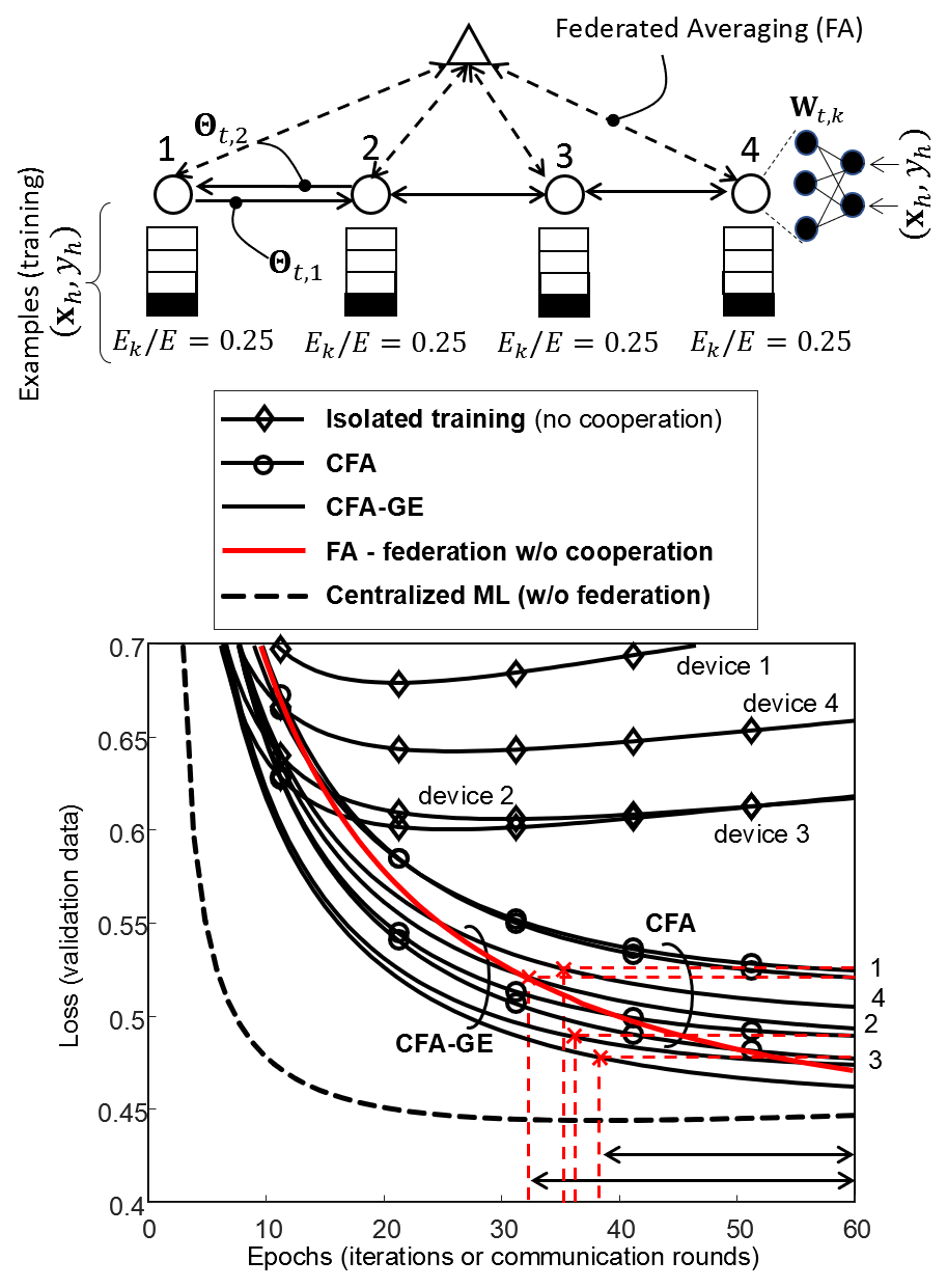
Figure 3: Comparison of FL methods over a multihop wireless network of $K=4$ devices. Validation loss vs. iterations over the full MNIST dataset for all devices: CFA (circle markers), CFA-GE (solid lines without markers), FA (red line), isolated model training (diamond markers), and centralized ML without federation (dashed line). Iterations correspond to epochs when running inside the server, or communication rounds when running consensus or FA.

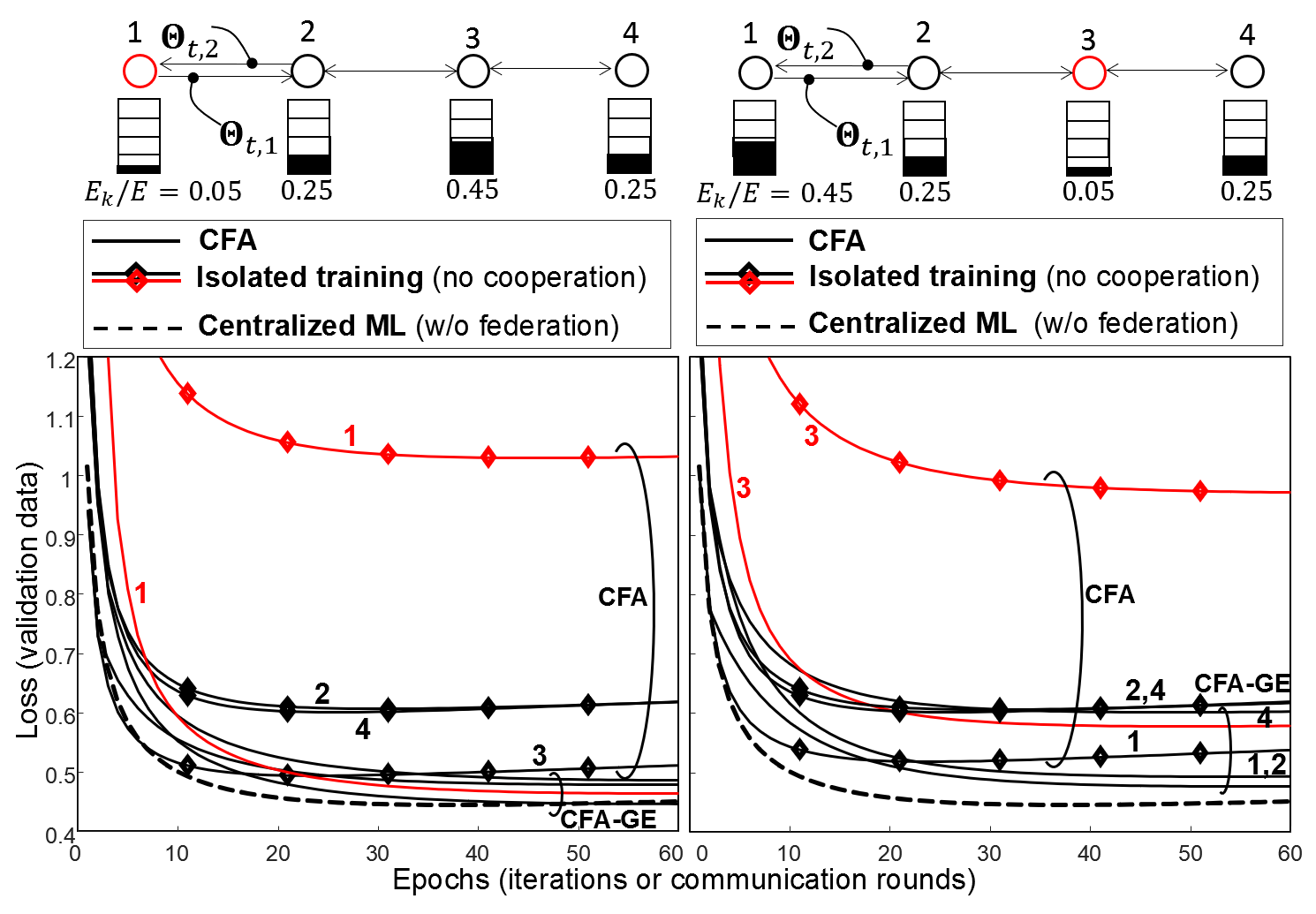
Figure 4: Effect of non-IID unbalanced training data over device $k=1$ and $k=3$ (red lines) of a multihop wireless network composed of $K=4$ devices. Validation loss over the full MNIST dataset vs. epochs (or consensus iterations). Comparison between CFA (solid lines), isolated model training (diamond markers), and centralized ML without federation (dashed line) is also presented. Non-IID data distribution is shown visually on top, for each case.

In Figs. 3-4, we validate the performances of the CFA algorithms in case of uniform (Fig. 3) and uneven (Fig. 4) data distribution among the devices. More specifically, Fig. 3 compares CFA and CFA-GE, with CFA-GE using the two-stage negotiation algorithm of Sect. III-C and starting at epoch $t=3$. On the other hand, in Fig. 4, we consider the general case where the data is unevenly distributed, while partitioning among devices is also non IID. Herein, we compare two cases. In the first one, device $1$ (Fig. 4 on the left) is located at the edge of the network and connected to one neighbor only. It obtains $E_{k}=80$ images from only $6$ of the available $C$ classes, namely the $5$% of the training database of $E$ images. Device $3$, connected with $2$ neighbors, retains a larger database ($E_{k}=720$ images, $45$% of the training database). In the second case (on the right), the situation is reversed. As expected, compared with the first case, convergence is more penalized in the second case, although CFA running on device $3$ (red lines) can still converge. As shown in Fig. 3, CFA-GE (solid lines without markers) further reduces the loss, compared with CFA (circle markers). Effect of an unbalanced database for CFA-GE is also considered in Sect. V.

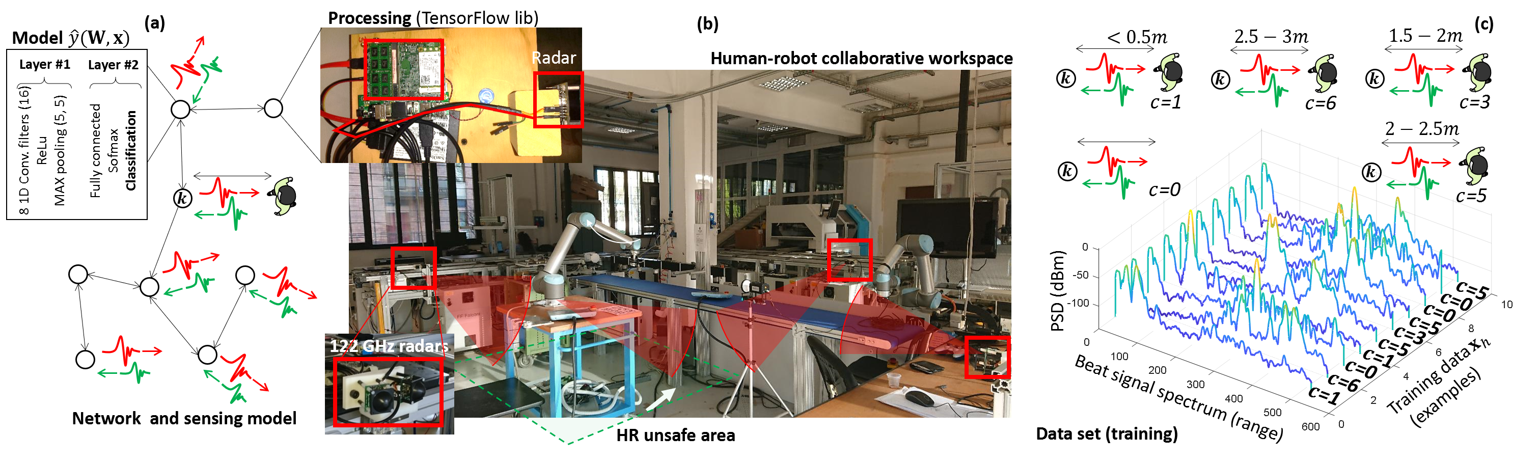
Figure 5: From left to right: a) experimental setup: network and sensing model for in-network federated learning with Convolutional Neural Network (CNN, top-left corner) examples whose parameters are shown in Table I; b) industrial scenario (CNR-STIIMA de-manufacturing pilot plant) and deployed radars; c) examples $\mathbf{x}_{h}$ of measured beat signal spectrum ($512$ point FFT) for selected classes ($c=0,1,3,5,6$).

FL and consensus schemes have been implemented using the TensorFlow library [33], while real-time D2D connectivity is simulated by a MonteCarlo approach. All simulations are running for a maximum of $60$ epochs. Besides the proposed consensus strategies, validation loss is also computed for three different scenarios. The first one is labelled as “isolated training” and it is evaluated in Fig. 3 for IID and in Fig. 4 for non IID data. In this scenario, $K=4$ models are trained without any cooperation from neighbors (or server) by using locally trained data only. This use case is useful to highlight the benefits of mutual cooperation that are significant after epoch $t=9$ for IID and after $t=3$ epochs for non IID, according to the considered network layout. Notice that isolated training is also limited by overfitting effects after iteration $t=30$, as clearly observable in Fig. 3 and in Fig. 4, since local/isolated model optimization is based only on few training images, compared with the validation database of $60.000$ images. Consensus and mutual cooperation among devices thus prevents such overfitting. The second scenario “centralized ML without federation” (dashed lines in Figs. 3 and 4) corresponds to (5) and gives the validation loss obtained when all nodes are sending all their locally trained data directly to the server. It serves as benchmark for convergence analysis as provides the optimal parameter set $\mathbf{W}$ considering $E=1.600$ images for training. Notice that the CFA-GE method closely approaches the optimal parameter set and converges faster than CFA. The third scenario implements the FA strategy (see Sect. II) that relies on server coordination, while cooperation among devices through D2D links is not enabled. As depicted in Fig. 3, the convergence of the FA validation loss is similar to those of devices $2$ and $3$, although convergence speed is slightly faster after epoch $t=55$. In fact, for the considered network layout, devices $2$ and $3$ can be considered a good replacement of the server, being directly connected with most of the devices. In the next section, we consider a more complex device deployment in a IIoT challenging scenario.

V Validation in an experimental IIoT scenario

The proposed in-network FL approaches of Sect. IV are validated here on a real-world IIoT use case. Data are partitioned over IIoT devices and D2D connectivity [14] is used here as a replacement to centralized communication infrastructure [34]. As depicted in Fig. 5, the reference scenario consists of a large-scale and dense network [35] of autonomous IIoT devices that are sensing their surroundings using Frequency Modulated Continuous Wave (FMCW) radars [45] working in the $122$ GHz (sub-Thz) band. Radars in the mmWave (or sub-THz) bands are very effective in industrial production lines (or robotic cells, as in Fig. 5.b) for environment/obstacle detection [36], velocity/distance measurement and virtual reality applications [43]. In addition, mmWave radios have been also considered as candidates for 5G new radio (NR) allocation. They thus represent promising solutions towards the convergence of dense communications and advanced sensing technologies [3].

In the proposed setup, the above cited devices are employed to monitor a shared industrial workspace during Human-Robot Collaboration (HRC) tasks to detect and track the position of the human operators (i.e., the range distance from the individuals) that are moving nearby a robotic manipulator inside a fenceless space [42]. In industrial shared workplaces, measuring positions and distance is mandatory to enforce a worker protection policy, to implement collision avoidance, reduction of speed, anticipating contacts of limited entity, etc. In addition, it is highly desirable that operators are set free from wearable devices to generate location information [3]. Tracking of body movements must also not depend on active human involvement. For static background, the problem of passive body detection and ranging can be solved via background subtraction methods, and ML tools (see [44] and references therein). The presence of the robot, often characterized by a massive metallic size, that moves inside the shared workplace, poses additional remarkable challenges in ranging and positioning, because robots induce large, non-stationary, and fast RF perturbation effects [42].

The radars collect a large amount of data, that cannot be shipped back to the server for training and inference, due to the latency constraints imposed by the worker safety policies. In addition, direct communication with the server is available but reserved to monitor the robot activities (and re-planning robotic tasks in case of dangerous situations) [42] and should not be used for data distribution. Therefore, to solve the scalability challenge while addressing latency, reliability and bandwidth efficiency, we let the devices perform model training without any server coordination but using only mutual cooperation with neighbors. We thus adopt the proposed in-network FL algorithms relying solely on local model exchanges over the D2D active links.

In what follows, we first describe the dataset and the ML model $\hat{y}(\mathbf{W};\mathbf{x})$ adopted for body motion recognition. Next, we investigate the convergence properties of CFA and CFA-GE solutions, namely the required number of communication rounds (i.e., latency) for varying connectivity layouts, network size and hyper-parameters choices, such as mixing weights and step sizes. Finally, we provide a quantitative evaluation of the communication overhead and of the local computational complexity comparing all proposed algorithms.

V-A Data collection and processing

In the proposed setup, the radar (see [43] for a review) transmitting antennas radiate a sweeped modulated waveform [45] with bandwidth equal to $6$ GHz, carrier frequency $119$ GHz, and ramp (pulse) duration set to $T=1$ ms. The radar echoes, reflected by moving objects are mixed at the receiver with the transmitted signal to obtain the beat signal. Beat signals are then converted in the frequency domain (i.e., beat signal spectrum) by using a $512$-point Fast Fourier Transform (FFT) and averaged over $10$ consecutive frames (i.e., frequency sweeps or ramps). FFT samples are used as model inputs $\mathbf{x}_{h}$ and serve as training data collected by the individual devices. The network of radars is designed to discriminate body movements from robots and, in turn, to detect the distance of the worker from the robot with the purpose of identifying potential unsafe conditions [36]. The ML model is here trained to classify $C=8$ potential HR collaborative situations characterized by different HR distances corresponding to safe or unsafe conditions. In particular, class $c=0$ (model output $\hat{y}=y_{0}$) corresponds to the robot and the worker cooperating at a safe distance (distance $\geq 3.5$ m), class $c=1$ ($\hat{y}=y_{1}$) identifies the human operator as working close-by the robot, at distance $<0.5$ m. The remaining classes are: $c=2$ ($0.5\leq$ distance $<1$ m), $c=3$ ($1\leq$ distance $<1.5$ m), $c=4$ ($1.5\leq$ distance $<2$ m), $c=5$ ($2\leq$ distance $<2.5$ m), $c=6$ ($2.5\leq$ distance $<3$ m), $c=7$ ($3\leq$ distance $<3.5$ m). The FFT range measurements (i.e., beat signal spectrum) and the corresponding true labels in Fig. 5.c, are collected independently by the individual devices and stored locally. During the initial FL stage, each device independently obtains $E_{k}=25$ FFT range measurements. Data distribution is also non-IID: in other words, most of the devices have local examples only for a (random) subset of the $C=8$ classes of the global model. However, we assume that there are sufficient examples for each class considering the data stored on all devices. Local datasets correspond to the $1$% of the full training database. Mini-batches for local gradients have size equal to $B=5$, training passes thus consist of $E_{k}/B=5$ mini-batches, for fast model update. On the contrary, validation data consists of $E=16.000$ range measurements collected inside the industrial plant.

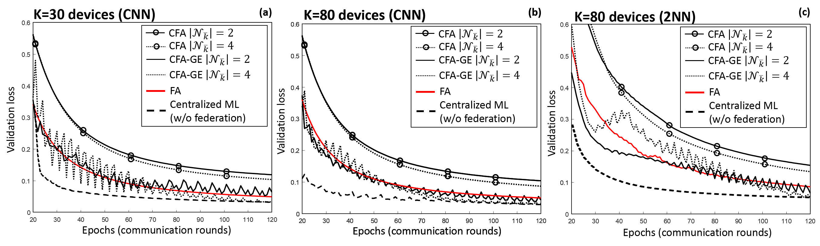
Figure 6: From left to right: a) FL for CNN model with $K=30$, b) $K=80$ devices and c) 2NN model with $K=80$ devices. The network is characterized by $\left|\mathcal{N}_{k}\right|=2$ (solid lines) and $\left|\mathcal{N}_{k}\right|=4$ (dotted lines) neighbors per node. Comparative analysis of CFA, CFA-GE, FA (red lines), and centralized ML i.e. learning w/o federation (dashed lines). CNN and 2NN parameters are described in Table I.

	CNN	2-NN
NN model	$\begin{array}[]{c}\textrm{8 1D conv. (16 taps)}\\ \downarrow\\ \textrm{ReLu}\\ \downarrow\\ \textrm{MaxPool (5, 5)}\\ \downarrow\\ \textrm{FC}(168\times C)\\ \downarrow\\ \textrm{Softmax}\end{array}$	$\begin{array}[]{c}\textrm{FC $(512\times 32)$}\\ \downarrow\\ \textrm{ReLu}\\ \downarrow\\ \textrm{FC}(32\times C)\\ \downarrow\\ \textrm{Softmax}\end{array}$
Layer $q=1$	$\mathbf{w}_{0,1}:\begin{array}[]{l}d_{1}=16\\ d_{2}=8\end{array}$	$\mathbf{w}_{0,1}:\begin{array}[]{l}d_{1}=512\\ d_{2}=32\end{array}$
	$\mathbf{w}_{1,1}$: $\begin{array}[]{c}d_{1}=8\end{array}$	$\mathbf{w}_{1,1}$: $\begin{array}[]{c}d_{1}=32\end{array}$
Layer $q=2$	$\mathbf{w}_{0,2}$: $\begin{array}[]{l}d_{1}=168\\ d_{2}=C\end{array}$	$\mathbf{w}_{0,2}$: $\begin{array}[]{l}d_{1}=32\\ d_{2}=C\end{array}$
	$\mathbf{w}_{1,2}$: $\begin{array}[]{c}d_{1}=C\end{array}$	$\mathbf{w}_{1,2}$: $\begin{array}[]{c}d_{1}=C\end{array}$

TABLE I: NN models and trainable parameters $\mathbf{W}$ (weights and biases) for $C=8$ classes.

Unlike the previous section, we now choose a ML global model characterized by a NN with $Q=2$ trainable layers. In particular, two networks are considered with hyper-parameters and corresponding dimensions for weights and biases $\mathbf{W}=\left[\mathbf{w}_{0,1}^{\mathrm{T}},\mathbf{w}_{1,1},\mathbf{w}_{0,2}^{\mathrm{T}},\mathbf{w}_{1,2}\right]$ that are detailed in Table I. The first convolutional NN model (CNN) consists of a 1D convolutional layer ($8$ filters with $16$ taps) followed by max-pooling (non trainable, size $5$ and stride $5$) and a fully connected (FC) layer of dimension $168\times C$. The second model (2NN) replaces the convolutional layer with an FC layer of $32$ hidden nodes (dimension $512\times 32$) followed by a ReLu layer and a second FC layer of dimension $32\times C$. The examples are useful to assess the convergence properties of the proposed distributed strategies for different layer types, dimensions and number of trainable parameters. As before, we further assume that, during the initial stage, each device has knowledge of the ML global model structure (see layers and dimensions in Table I). At each new communication round, model parameters for each layer are multiplexed and propagated simultaneously by using a Time Division Multiple Access (TDMA) scheme [14].

FL has been simulated on a virtual environment but using real data from the plant. This virtual environment creates an arbitrary number of virtual devices, each configured to process an assigned training dataset and exchanging parameters $\Theta_{t,k}$ that are saved in real-time on temporary cache files. Files may be saved on RAM disks to speed up the simulation time. The software is written in Python and uses TensorFlow and multiprocessing modules: simplified configurations for testing both CFA and CFA-GE setups are also provided in the repository [46]. The code script examples are available as open source and show the application of CFA and CFA-GE for different NN models. Hyper-parameters such as learning rates for weights $\alpha_{k,i}$, gradients $\mu_{t}\beta_{k,i}$, number of neighbors $\mathcal{N}_{\overline{k}}$ and $\varrho$ in (17) are fully configurable. The data-sets obtained in the scenario of Fig. 5.b are also available in the same repository. Finally, examples have been provided for implementation and analysis of execution time on low power devices (Sect. V-C). The current optimization toolkit does not simulate, or account for, packet losses during communication: this is considered as negligible for short-range connections. However, the network and connectivity can be time-varying and arbitrarily defined.

Configuration (1)	Configuration (2)	Configuration (3)
$\begin{array}[]{l}K<15\\ \left|\mathcal{N}_{\bar{k}}\right|\leq 6\end{array}$	$\begin{array}[]{l}K\in\left[15,50\right]\\ \left|\mathcal{N}_{\bar{k}}\right|\in\left[2,6\right]\end{array}$	$\begin{array}[]{l}K>50\\ \left|\mathcal{N}_{\bar{k}}\right|=2\end{array}$
CFA
$\begin{array}[]{l}\epsilon_{t}=1\\ \mu_{t}=0.025\\ \alpha_{k,i}\>\textrm{in }(\ref{eq:mix})\end{array}$	$\begin{array}[]{l}\epsilon_{t}=0.5\\ \mu_{t}=0.025\\ \alpha_{k,i}\>\textrm{in }(\ref{eq:mix})\end{array}$	$\begin{array}[]{l}\epsilon_{t}=0.5\\ \mu_{t}=0.025\\ \alpha_{k,i}\>\textrm{in }(\ref{eq:mix})\end{array}$
CFA-GE
$\begin{array}[]{l}\mu_{t}\beta_{k,i}\leq 0.15\\ \varrho=0.99\\ \textrm{(MEWMA)}\end{array}$	$\begin{array}[]{l}\mu_{t}\beta_{k,i}\in\left[.1,.15\right]\\ \varrho=0.95\div 0.99\\ \textrm{(MEWMA)}\end{array}$	$\begin{array}[]{l}\mu_{t}\beta_{k,i}\leq 0.1\\ \varrho=0.9\div 0.95\\ \textrm{(MEWMA)}\end{array}$

TABLE II: Optimized hyper-parameters for CFA and CFA-GE.

V-B Gradient exchange optimization for NN

In what follows, FL is verified by varying the number of devices $K=30\div 80$ and number of neighbors $\left|\mathcal{N}_{\overline{k}}\right|=2\div 10$ to test different D2D connectivity layouts. In Figure 6, we validate the consensus based FL tool, for both CNN and 2NN models, over networks with increasing number of devices from $K=30$ to $K=80$. To simplify the analysis of different connectivity scenarios, the network is simulated as k-regular (i.e., all network devices have the same number of neighbors, or degree) while we verify realistic topologies characterized by $\left|\mathcal{N}_{\bar{k}}\right|=2,4,6,10$ neighbors per node. First, in Fig. 6, we compare decentralized CFA and CFA-GE with FA and conventional centralized ML without federation in (5). The chosen optimization hyper-parameters are summarized in Table II. For all FL cases (CFA, CFA-GE and FA), we plot the validation loss vs. communication rounds (i.e., epochs) averaged over all $K$ devices. For centralized ML (dashed lines), validation loss is analyzed over epochs now running inside the server. The CFA plots (circle markers) approach slowly the curve corresponding to FA and centralized ML, while performance improves in dense networks (dotted lines). CFA-GE curves (solid and dotted lines without markers) are comparable with FA, and converge after $50-60$ communication rounds. Use of $\left|\mathcal{N}_{\bar{k}}\right|=2$ neighbors (solid lines) is sufficient to approach FA performances. Increasing the number of neighbors to $\left|\mathcal{N}_{\bar{k}}\right|=4$ (dotted lines) makes the validation loss comparable with the centralized ML without federation. Running local SGD on received gradients as in eq. (19) causes some fluctuations of the validation loss as approaching convergence. Fluctuations are due to the (large) step size $\mu_{t}\beta_{k,i}$ used to combine the gradients every communication round: learning rate adaptation techniques [10] can be applied for fine tuning. Considering the 2NN model, validation loss is larger for all cases as the result of the larger number of model parameters to train, compared with CNN. CFA-GE is still comparable with FA mostly after $70$ rounds and converges towards centralized ML after $110$ rounds. In all cases, $\left|\mathcal{N}_{\bar{k}}\right|=2$ neighbors are sufficient to approach FA results. More neighbors provide performance improvements mostly in small networks ($K=30$ devices), while it is still useful to match centralized ML performances.

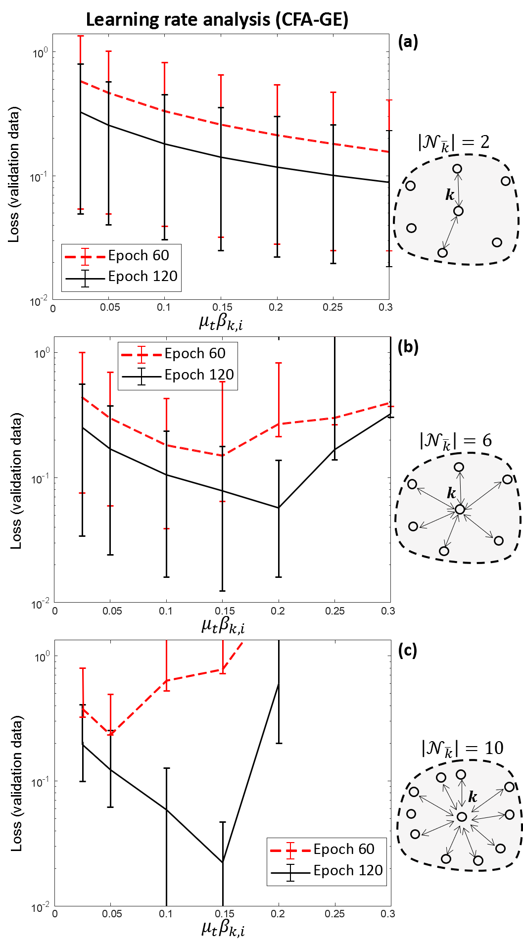
Figure 7: From top to bottom: validation loss for varying rates ($\mu_{t}\beta_{k,i}$) for $K=80$ devices and k-regular networks with varying connectivity, ranging from a) $\left|\mathcal{N}_{\bar{k}}\right|=2$, b) $\left|\mathcal{N}_{\bar{k}}\right|=6$ up to c) $\left|\mathcal{N}_{\bar{k}}\right|=10$.

In Fig. 7, we consider the CFA-GE method and analyze more deeply the effect of the hyper-parameter choice on convergence, for $K=80$ devices and varying network degrees $\left|\mathcal{N}_{\bar{k}}\right|$. The first case ($\left|\mathcal{N}_{\bar{k}}\right|=2$) is representative of a multihop wireless network; networks with larger degrees ($\left|\mathcal{N}_{\bar{k}}\right|=6$, $\left|\mathcal{N}_{\bar{k}}\right|=10$) are useful to verify the performance of FL over denser networks. Line plots with bars in Fig. 7 are used to graphically represent the variability of the validation loss observed by the devices. We analyze the learning rate ($\mu_{t}\beta_{k,i}$) used to combine the gradients received from the neighbors in (19). Other hyper-parameters are selected as in Table II. As expected, increasing the network degree helps convergence and makes the validation loss to decrease faster since less communication rounds are required. However, while for $\left|\mathcal{N}_{\bar{k}}\right|=2$ degree networks the learning rates $\mu_{t}\beta_{k,i}$ can be chosen arbitrarily in the range $\mu_{t}\beta_{k,i}=0.1\div 0.2$ without affecting performance, denser networks, i.e., with large degree $\left|\mathcal{N}_{\bar{k}}\right|=10$, require the optimization of the learning rate: smaller rates $\mu_{t}\beta_{k,i}\leq 0.1$ improve convergence for $\left|\mathcal{N}_{\bar{k}}\right|=6$ and $\left|\mathcal{N}_{\bar{k}}\right|=10$.

In Table III, we analyze the latency of the FL process that is measured here in terms of number of communication rounds. CFA-GE is considered in detail, while performance of CFA can be inferred from Fig. 6. The Table III reports the number $(t$) of communication rounds (or epochs) that are required to achieve a target validation loss for all devices, such that $L_{t,k}^{(val)}\leq 0.5$, $\forall k$. For the considered case, the chosen validation loss of $0.5$ corresponds to a (global) accuracy of $\gamma_{G}=0.9$. Focusing on CNN layers, a network with $\left|\mathcal{N}_{\bar{k}}\right|=2$ neighbors per device requires a max of $21$ communication rounds (and a minimum of $9$) to achieve a target loss of $L_{t,k}^{(val)}\leq 0.5$. This is in line with the theoretical bound [24] $\log\left[\mathrm{1/\left(1-\gamma_{G}\right)}\right]\mathrm{/\gamma_{L}}=15$ for local accuracy $\gamma_{L}\simeq 0.2$ (obtained by isolated training). Considering FA (not shown in the Table), the number of required rounds ranges from $7$ to $16$, and it is again comparable with decentralized optimization. Increasing the number of neighbors to $\left|\mathcal{N}_{\bar{k}}\right|=6$, the required communication rounds reduce to $18$ and to $14$ for $\left|\mathcal{N}_{\bar{k}}\right|=10$. For 2NN layers, the required number of epochs increases due to the smaller local accuracy $\gamma_{L}\simeq 0.1$ as well as the larger number of parameters to be trained for each NN layer. Finally, for the proposed setup, we noticed that performance improves by keeping the learning rate $\mu_{t}\beta_{k,i}$ for the hidden layer parameters $\left[\mathbf{w}_{0,1}^{\mathrm{T}},\mathbf{w}_{1,1}\right]$, ($q=1$) slightly larger than the rate for the output layer parameters $\left[\mathbf{w}_{0,2}^{\mathrm{T}},\mathbf{w}_{1,2}\right]$, ($q=2$). This is particularly evident when convolutional layers are used.

	Layers	CNN ($L_{t,k}^{(val)}\leq 0.5$)		2NN ($L_{t,k}^{(val)}\leq 0.5$)
$\left|\mathcal{N}_{\bar{k}}\right|$	$(\mathbf{W})$	$\mu_{t}\beta_{k,i}$	Epochs ($t$)	$\mu_{t}\beta_{k,i}$	Epochs ($t$)
			(min | max)		(min | max)
$2$	$q=1$	$\mathbf{0.2}$	$9$ | $\mathbf{21}$	$0.05$	$11$ | $51$
	$q=2$	$\mathbf{0.15}$		$0.1$
	$q=1$	$0.15$	$10$ | $26$	$\mathbf{0.1}$	$12$ | $\mathbf{23}$
	$q=2$	$0.2$		$\mathbf{0.05}$
$6$	$q=1$	$\mathbf{0.15}$	$8$ | $\mathbf{18}$	$0.025$	$17$ | $28$
	$q=2$	$\mathbf{0.1}$		$0.05$
	$q=1$	$0.1$	$12$ | $23$	$\mathbf{0.05}$	$11$ | $\mathbf{19}$
	$q=2$	$0.15$		$\mathbf{0.025}$
$10$	$q=1$	$\mathbf{0.05}$	$7$ | $\mathbf{14}$	$0.025$	$15$ | $23$
	$q=2$	$\mathbf{0.025}$		$0.02$5
	$q=1$	$0.025$	$11$ | $\mathbf{17}$	$\mathbf{0.05}$	$10$ | $\mathbf{17}$
	$q=2$	$0.05$		$\mathbf{0.025}$

TABLE III: Communication rounds (epochs $t$) for target validation loss: $L_{t,k}^{(val)}\leq 0.5$, $\forall k$. Min. and max. epochs over $K=80$ devices for CNN and 2NN. Optimized parameters (bold) are shown, too.

V-C Communication and computational cost assessment

The CFA-GE method achieves the performance of the centralized ML without federation, in exchange for a more intensive use of D2D wireless links and local computations, that scale in both cases with the number of neighbors $\left|\mathcal{N}_{\bar{k}}\right|$. Based on the the analysis in Sect. III-D, in Table IV we compare the communication overhead and computational cost for varying number of neighbors $\left|\mathcal{N}_{k}\right|$, considering FA, CFA and CFA-GE methods. In particular, the communication overhead quantifies the number of bytes that need to be transmitted over-the-air by each device every communication/consensus round. The computational cost is measured in terms of average local execution time per communication round and device.

The communication overhead of FA and CFA is $2.98$ Kbyte/round/device for CNN and $33.36$ Kbyte/round/device for 2NN. Overhead corresponds in both cases to the model $\mathbf{W}$ size: this is evaluated according to the model parameters highlighted in Table I and assuming $16$ bit/parameter quantization. CFA-GE overhead is larger as it scales linearly with $\left|\mathcal{N}_{k}\right|$, therefore it can be quantified as $2.98\cdot\left|\mathcal{N}_{k}\right|$ Kbyte/round/device for CNN and $33.36\cdot\left|\mathcal{N}_{k}\right|$ Kbyte/round/device for 2NN. Notice that bandwidth-limited communication systems, e.g., based on IEEE 802.15.4, 6LoWPAN and related evolutions [14]-[34], are characterized by small physical frame payloads, typically below $1$ Kbyte/frame. Therefore, sending FA, CFA or CFA-GE parameters on each round might require the aggregation of consecutive physical frames, or multiple network layer transactions. For comparison with centralized ML, FFT training measurements collected individually by devices have size within the range $1\div 4$ Mbyte, assuming $32$ bit quantization for in-phase (I) and quadrature (Q) components.

Local execution time considers here the ML stages only, while data pre-processing and acquisition steps are not included, being negligible compared to the learning steps. The execution time shown in Table IV is measured using the timeit Python module, on a device equipped with a $1.5$ GHz quad core ARM Cortex-A72 processor with 4 GB internal RAM. Focusing on a realistic IIoT environment, the device has thus limited computational capabilities, compared with the server. Execution time depends in general on the specific CPU or Tensor Processing Unit (TPU) performances; nevertheless, the analysis of the results in Table IV is useful to highlight the scaling performance of the proposed methods compared to the plain FA algorithm. Considering FA, the execution time on the device is ruled by local SGD rounds: it is $140$ms and $145$ms for CNN and 2NN, respectively. Notice that FA needs the server for aggregation, while such additional cost is not considered here. Compared with FA, CFA adds a model aggregation stage (8) for each NN layer that takes $0.5$ ms on average per neighbor. Finally, CFA-GE adds a cumulative time of $90$ ms for CNN and $94$ ms for 2NN on average per neighbor. This is needed for the computation of one additional gradient, the MEWMA update (17), and one SGD round (19) per neighbor.

Considering both overhead and local execution time, CFA-GE cost per round is higher compared with CFA and FA and scales almost linearly with the number of neighbors $\left|\mathcal{N}_{\bar{k}}\right|$. CFA total cost is instead comparable with FA when $\left|\mathcal{N}_{\bar{k}}\right|<10$. However, it is worth to notice that, as shown by the numerical results in Sect. V-B, CFA-GE only needs $\left|\mathcal{N}_{\bar{k}}\right|=2$ neighbors for convergence and even with such a low degree of cooperation it reduces the number of rounds by almost one order of magnitude (Fig. 6) compared to CFA. Using more than $\left|\mathcal{N}_{\bar{k}}\right|=2$ cooperating neighbors for CFA-GE provides only marginal improvements and it is thus not recommended. Having said that, we can conclude that CFA-GE is promising as an effective replacement for FA and centralized ML when it is critical to limit the number of communication rounds, or in case frequent learning updates are needed. CFA keeps complexity and overhead comparable with FA in exchange for more rounds. It is thus suitable for non-critical learning tasks and it can support bandwidth-limited D2D communication systems characterized by small frame payloads.

	Comm. overhead			Execution time (avg.)
	[Kbyte/round/device]			[m.sec./round/device]
$\left|\mathcal{N}_{\bar{k}}\right|$		CNN	2NN	CNN	2NN
$2$	FA	$2.98$	$33.36$	$140$ms	$145$ms
	CFA	$2.98$	$33.36$	$141$ms	$146$ms
	CFA-GE	$5.96$	$66.72$	$321$ms	$334$ms
$6$	FA	$2.98$	$33.36$	$140$ms	$145$ms
	CFA	$2.98$	$33.36$	$142$ms	$147$ms
	CFA-GE	$17.88$	$200.16$	$684$ms	$711$ms
$10$	FA	$2.98$	$33.36$	$140$ms	$145$ms
	CFA	$2.98$	$33.36$	$149$ms	$153$ms
	CFA-GE	$29.8$	$333.7$	$984$ms.	$\sim 1$sec.

TABLE IV: Communication overhead [Kbyte/round/device] and computational cost - average execution time [m.sec./round/device] measured on the device.

VI Conclusions and open problems

The paper addressed a new family of FL methods that leverage the mutual cooperation of devices in distributed wireless IoT networks without relying on the support of a central coordinator. The adaptation of federated averaging, namely the CFA method, was first discussed to exploit distributed consensus paradigms for FL. Next, to improve convergence speed, we proposed a new algorithm based on iterative exchange of model updates and gradients. The CFA-GE algorithm was optimized for two-stage gradient negotiations so that it can be tailored to arbitrarily large scale networks.

The proposed distributed learning approach was validated on an IIoT scenario where a NN model was distributedly trained to solve the problem of passive body detection inside a human-robot collaborative workspace. CFA-GE was shown to achieve the performance of server-side (or centralized) federated optimization. Decentralized optimization is fully server-less with respect to NN model training as intelligence is pushed down into the IoT devices. This is particularly effective when direct communication with the infrastructure is reserved for critical tasks (e.g., to control the robot or to perform safety tasks). Motivated by the growing range of ML applications that will be deployed in 5G and beyond wireless networks, FL via consensus emerges in this paper as a promising framework for flexible model optimization over networks characterized by decentralized connectivity patterns as in massive IoT implementations.

Despite the promising features, the proposed consensus based approach is giving rise to new challenges, which need to be taken into account during the system deployment. For example, the paper considered a simple enough NN model for optimization running on IoT devices with limited computation capabilities. However, training of deeper networks on constrained devices is expected to become the mainstream in the near future [48]. Application of consensus based federated optimization to deeper networks might require a more efficient use of the limited bandwidth, including quantization, compression or ad-hoc channel encoding [47]. As revealed in the considered case study, tweaking of the model hyper-parameters [16] as well as optimizing the learning rates for each NN model layer separately are also viable solutions to limit the number of communication rounds. Finally, although the paper addressed a classification task as application of federated optimization, both CFA and CFA-GE can be generalized to perform a wider range of computations.

Appendix

Appendix A: Comparing CFA and CFA-GE

Combining (13) and (14), we obtain the update equation for CFA-GE

$$\begin{array}[]{c}\mathbf{W}_{t+1,k}=\underset{\widetilde{\boldsymbol{\psi}}_{t,k}}{\underbrace{\boldsymbol{\psi}_{t,k}-\mu_{t}\sum_{i\in\mathcal{N}_{\bar{k}}}\beta_{t,i}\nabla L_{t,i}\left(\boldsymbol{\psi}_{t,k}\right)}-}\\ -\mu_{t}\beta_{t,k}\left[\nabla L_{t,k}\left(\widetilde{\boldsymbol{\psi}}_{t,k}\right)\right]\end{array}$$ (22)

with $\boldsymbol{\psi}_{t,k}$ in (8). This is comparable with the CFA approach in (9). Unlike CFA, gradient exchange terms $\sum_{i\in\mathcal{N}_{\bar{k}}}\beta_{t,i}\nabla L_{t,i}\left(\boldsymbol{\psi}_{t,k}\right)$ allow to incorporate the influence of training data collected by the neighborhood of device $k$ through the gradient terms $L_{t,i}\left(\boldsymbol{\psi}_{t,k}\right)$. Computation of $\widetilde{\boldsymbol{\psi}}_{t,k}$ (13) thus corresponds to an initial gradient descent round using the training data from the neighborhood, while subsequent rounds (22) are performed using SGD over local data mini-batches.

Appendix B: Application to SGD with momentum

SGD is considered throughout the paper as a popular optimization strategy; however it shows slow convergence properties in some ML problems [10]. Recently, the method of momentum inspired several algorithms (such as RMSProp and Adam [41]) optimized for accelerated learning. Considering that in federated optimization any improvement in the convergence speed is beneficial in terms of bandwidth usage and latency, we address the necessary adaptations of CFA-GE strategy to leverage momentum information. With respect to SGD, momentum addresses the problem of imperfect estimation of the stochastic gradients as well as the conditioning of the Hessian matrix [32]. Poor estimation of gradients is even more critical when considering distributed learning setups. Compared with SGD, the use of momentum modifies the local update rule (9),(14) as

$$\begin{cases}\begin{array}[]{c}\mathbf{W}_{t+1,k}=\boldsymbol{\psi}_{t,k}+\mathbf{\nu}_{t+1,k}\\ \mathbf{\nu}_{t+1,k}=\varrho\mathbf{\nu}_{t,k}-\mu_{t}\nabla L_{t,k}(\boldsymbol{\psi}_{t,k})\end{array}\end{cases}$$ (23)

where both current and past gradients contribute to the local model update (for device $k)$ as multiplied by an exponentially decaying function ruled by hyper-parameter $\varrho\in\left[0,1\right)$. $\mathbf{\nu}_{t,k}$ is the momentum, or velocity, of the gradient descent particle at round $t$, that is stored by device $k$.

Momentum based techniques can be used seamlessly combined with CFA by simply replacing (9) with (23) as gradient sharing is not permitted. Considering that in CFA-GE local gradients are exchanged among neighbors, some necessary adaptations are required to leverage momentum. The received gradients, i.e. at epoch $t-1$, are now used for local momentum update as

$$\mathbf{\nu}_{t,k}=\varrho\mathbf{\nu}_{t-1,k}-\mu_{t}\sum_{i\in\mathcal{N}_{\bar{k}}}\beta_{k,i}\mathcal{P}_{\Theta}\left[\overline{\nabla L}_{t-1,i}\right].$$ (24)

We then replace (19) with $\widetilde{\boldsymbol{\psi}}_{t,k}=\boldsymbol{\psi}_{t,k}+\mathbf{\nu}_{t,k}$ and (14) with (23). The use of the Nesterov momentum [32] policy requires minor adaptations: the devices should now exchange the parameters $\Theta_{t,k}:=\left[\boldsymbol{\psi}_{t,k}+\varrho\mathbf{\nu}_{t-1,k},\nabla\mathbf{L}_{t,k}\right].$ These are: the local model $\boldsymbol{\psi}_{t,k}+\varrho\mathbf{\nu}_{t-1,k}$ after applying the velocity term (24) and the gradients $\nabla\mathbf{L}_{t,k}:=\left\{\overline{\nabla L}_{t,k}(\mathbf{\boldsymbol{\psi}}_{t-1,i}),\text{}\forall i\in\mathcal{N}_{\bar{k}}\right\}$ described as

$$\begin{array}[]{cccc}\overline{\nabla L}_{t,k}(\boldsymbol{\psi}_{t-1,i})&=&\varrho\nabla L_{t,k}(\boldsymbol{\psi}_{t-1,i}+\varrho\mathbf{\nu}_{t-1,i})+\\ &&+(1-\varrho)\overline{\nabla L}_{t-1,k},\end{array}$$ (27)

that replace the terms in eq. (17).

Appendix C: Description of Python scripts and datasets

The section describes the database that contains the range measurements obtained from FMCW THz radars inside the Human-Robot (HR) workspace. It also gives examples about how to use the sample Python code that implements the federated learning stages via consensus. The database is located in the folder $\mathrm{dati_{-}radar_{-}05-07-2019}$ and can be easily imported through Python:

⬇

import scipy.io as sio

db = sio.loadmat(’dati_radar_05-07-2019

/data_base_all_sequences_random.mat’)

The database contains 5 files:

i) Data_test_2.mat has dimension 16000 x 512. Contains 16000 FFT range measurements (512-point FFT of beat signal after DC removal) used for test. The corresponding labels are in label_test_2.mat

⬇

x_val = db(’Data_test_2’)

x_val_l = db(’label_test_2’)

ii) Data_train_2.mat has dimension 16000 x 512. Contains 16000 FFT range measurements (512-point FFT of beat signal after DC removal) used for training. The corresponding labels are in lable_train_2.mat

⬇

x_t = db(’Data_train_2’)

x_l = db(’label_train_2’)

iii) label_test_2.mat with dimension 16000 x 1, contains the true labels for test data (Data_test_2.mat), namely classes (true labels) correspond to integers from 0 to 7. Class 0: human worker at safe distance >3.5m from the radar (safe distance) Class 1: human worker at distance (critical) <0.5m from the corresponding radar Class 2: human worker at distance (critical) 0.5m - 1m from the corresponding radar Class 3: human worker at distance (critical) 1m - 1.5m from the corresponding radar Class 4: human worker at distance (safe) 1.5m - 2m from the corresponding radar Class 5: human worker at distance (safe) 2m - 2.5m from the corresponding radar Class 6: human worker at distance (safe) 2.5m - 3m from the corresponding radar Class 7: human worker at distance (safe) 3m - 3.5m from the corresponding radar.

iv) label_train_2.mat with dimension 16000 x 1, contains the true labels for train data (Data_train_2.mat), namely classes (true labels) correspond to integers from 0 to 7. See item (iii) for class descriptions.

v) permut.mat (1 x 16000) contains the chosen random permutation for data partition among nodes/device and federated learnig simulation (see python code)

Python code

Usage example for federated_sample_XXX_YYY.py.

• XXX refers to the ML model. Available options: CNN, 2NN

• YYY refers to the consensus-based federated learning method. Available options: CFA, CFA-GE.

Run

python federated_sample_XXX_YYY.py -h

for help. CFA and CFA-GE are described in Sect. III.A, and Sect. III.B, respectively. The code implements the two-stage implementation of CFA-GE (Sect. III.C).

For CNN network and CFA-GE use: federated_sample_CNN_CFA-GE.py [-h] [-l1 L1] [-l2 L2] [-mu MU] [-eps EPS] [-K K] [-N N] [-T T] [-ro RO]

For 2-NN network and CFA-GE use: federated_sample_2NN_CFA-GE.py [-h] [-l1 L1] [-l2 L2] [-mu MU] [-eps EPS] [-K K] [-N N] [-T T] [-ro RO]

Arguments:

-l1: l1 sets the learning rate (gradient exchange) for convolutional layer

-l2: l2 sets the learning rate (gradient exchange) for FC layer

-mu: mu sets the learning rate for local SGD

-eps: eps sets the mixing parameters for model averaging (CFA)

-K: K sets the number of network devices

-N: N sets the number of neighbors per device

-T T sets the number of training epochs

-ro ro sets the hyperparameter for MEWMA

Optional arguments:

-h, –help show this help message and exit.

For testing CFA performance with CNN network, please use:

federated_sample_CNN_CFA.py [-h] [-mu MU] [-eps EPS] [-K K] [-N N] [-T T]

Similarly, for 2-NN network, please use:

federated_sample_2NN_CFA.py [-h] [-mu MU] [-eps EPS] [-K K] [-N N] [-T T]

Optional arguments:

-h, –help show this help message and exit

-mu MU sets the learning rate for local SGD

-eps EPS sets the mixing parameters for model averaging (CFA)

-K K sets the number of network devices

-N N sets the number of neighbors per device

-T T sets the number of training epochs

Example 1:

⬇

python federated_sample_CNN_CFA-GE.py

-l1 0.025 -l2 0.02 -K 40 -N 2

-T 40 -ro 0.99

Use convolutional layers followed by a FC layer (see Table I, CNN network). Sets gradient learning rate for hidden layer to 0.025, for output layer to 0.02, K=40 devices, N=2 neighbors per device, MEWMA parameter 0.99 (see Sect. III).

Example 2:

⬇

python federated_sample_2NN_CFA-GE.py

-l1 0.01 -l2 0.015 -N 2 -T 40 -ro 0.99

Use FC layers only (see Table I, 2-NN network). Sets gradient learning rate for hidden layer to 0.01, for output layer to 0.015, K=80 devices (default), N=2 neighbors per device, MEWMA parameter 0.99.

Python package description

Python package can be downloaded also from https://test.pypi.org/project/consensus-stefano/0.3/.

To initialize CFA use the constructor:

consensus_p = CFA_process(federated, tot_devices, device_id, neighbors_number).

Use similar constructor for CFA-GE:

consensus_p = CFA-ge_process(federated, tot_devices, device_id, neighbors_number, ro).

Example:

⬇

consensus_p = CFA_process(True, 80, 2, 2)

Initialize CFA process on device 2 with 2 neighbors and for a network of 80 devices.

To apply/update federated weights use: consensus_p.getFederatedWeight( … )

To enable/disable consensus (dynamically) consensus_p.disable_consensus( … True/False … )

Changing ML network parameters

ML network parameters are defined in the Python scripts federated_sample_XXX_YYY.py. In particular considering CFA-GE script, the CNN network is defined at lines 99-109 by

⬇

# Construct model

# Layer #1 CNN 1d,

# Layer #2 FC

hidden0 = conv1d(x, W_ext_l1, b_ext_l1)

hidden01 = tf.layers.max_pooling1d(

hidden0, pool_size=stride,

strides=stride, padding=’SAME’)

fc01 = tf.reshape(hidden01,

[-1, multip*number])

pred = tf.nn.softmax(

tf.matmul(fc01, W_ext_l2) + b_ext_l2)

with parameters defined in lines 39-45. Modify these lines to change the CNN network, namely changing filter and stride sizes, or adding further layers.

References

- [1] C. Zhang, P. Patras. H. Haddadi, “Deep Learning in Mobile and Wireless Networking: A survey,” IEEE Comm. Surveys and Tutorials, vol. 21, no. 3, pp. 2224-2287, third-quarter 2019. doi: 10.1109/COMST.2019.2904897.
- [2] W. G. Hatcher and W. Yu, “A Survey of Deep Learning: Platforms, Applications and Emerging Research Trends,” IEEE Access, vol. 6, pp. 24411-24432, 2018.
- [3] S. Savazzi, S. Sigg, F. Vicentini, S. Kianoush and R. Findling, “On the Use of Stray Wireless Signals for Sensing: A Look Beyond 5G for the Next Generation of Industry,” Computer, vol. 52, no. 7, pp. 25-36, July 2019.
- [4] K. M. Alam and A. El Saddik, “C2PS: A Digital Twin Architecture Reference Model for the Cloud-Based Cyber-Physical Systems,” IEEE Access, vol. 5, pp. 2050-2062, 2017.
- [5] Samarakoon, M. Bennis, W. Saad, M. Debbah, “Federated Learning for Ultra-Reliable Low-Latency V2V Communication,” Proc. of the IEEE Globecom 2018.
- [6] M. Bennis, M. Debbah and H. V. Poor, “Ultrareliable and Low-Latency Wireless Communication: Tail, Risk, and Scale,” Proc. of the IEEE, vol. 106, no. 10, pp. 1834-1853, Oct. 2018.
- [7] KonečnÃœ J., et al., “Federated optimization: Distributed machine learning for on-device intelligence,” CoRR, 2016. [Online]. Available: http://arxiv.org/abs/ 1610.02527.
- [8] S. Wang et al., “Adaptive Federated Learning in Resource Constrained Edge Computing Systems,” IEEE Journal on Sel. Areas in Comm., vol. 37, no. 6, pp. 1205-1221, June 2019.
- [9] KonečnÃœ J., et al. “Federated learning: Strategies for improving communication efficiency,” CoRR, 2016. [Online]. Available: http://arxiv.org/abs/ 1610.05492.
- [10] L. Bottou, “Large-Scale Machine Learning with Stochastic Gradient Descent,” Proceedings of COMPSTAT, Physica-Verlag HD, 2010.
- [11] G. Aloi, et al., “The SENSE-ME platform: Infrastructure-less smartphone connectivity and decentralized sensing for emergency management,” Pervasive and Mobile Comput., vol. 42, 2017, Pages 187-208, ISSN 1574-1192.
- [12] S. Kianoush, M. Raja, S. Savazzi and S. Sigg, “A cloud-IoT platform for passive radio sensing: Challenges and application case studies,” IEEE Internet of Things Journal, vol. 5, no. 5, pp. 3624-3636, Oct. 2018.
- [13] M. Brambilla, M. Nicoli, G. Soatti, F. Deflorio, “Augmenting Vehicle Localization by Cooperative Sensing of the Driving Environment: Insight on Data Association in Urban Traffic Scenarios,” IEEE Transactions on Intelligent Transportation Systems, 2019.
- [14] L. Ascorti, et al., “A Wireless Cloud Network Platform for Industrial Process Automation: Critical Data Publishing and Distributed Sensing,” IEEE Trans. on Instrumentation and Measurement, vol. 66, no. 4, pp. 592-603, April 2017.
- [15] McMahan, et al. “Communication-efficient learning of deep networks from decentralized data,” Proc. of the 20th Int. Conf. on Artificial Intel. and Stat., pp. 1273–1282, vol. 54, 2017.
- [16] E. Jeong, et al. “Communication-Efficient On-Device Machine Learning: Federated Distillation and Augmentation under Non-IID Private Data,” NIPS Workshop, Montreal, Canada, 2018.
- [17] M. Blot, et al., “Gossip training for deep learning,” 30th Conference on Neural Information Processing Systems (NIPS), Barcelona, Spain, 2016. [Online]. Available: https://arxiv.org/abs/1611.09726.
- [18] J. A Daily, et al. “Gossipgrad: Scalable deep learning using gossip communication based asynchronous gradient descent,” [Online]. Available: https://arxiv.org/abs/1803.05880.
- [19] A. Guha, S. Siddiqui, S. Polsterl, N. Navab, and C. Wachinger, “BrainTorrent: A Peer-to-Peer Environment for Decentralized Federated Learning,” [Online]. Available: https://arxiv.org/abs/1905.06731.
- [20] C. Hu, J. Jiang, Z. Wang, “Decentralized Federated Learning: A Segmented Gossip Approach,” 1st International Workshop on Federated Machine Learning for User Privacy and Data Confidentiality (FML’19) [Online]. Available: https://arxiv.org/abs/1908.07782.
- [21] A. Lalitha, S. Shekhar, T. Javidi, F. Koushanfar, “Fully decentralized federated learning,” 3rd Workshop on Bayesian Deep, NIPS Workshop, 2018.
- [22] A. Lalitha, O. C. Kilinc, T. Javidi, F. Koushanfar, “Peer-to-peer Federated Learning on Graphs,” [Online]. Available: https://arxiv.org/abs/1901.11173.
- [23] G. Soatti, M. Nicoli, S. Savazzi and U. Spagnolini, “Consensus-Based Algorithms for Distributed Network-State Estimation and Localization,” IEEE Trans. on Signal and Information Processing over Networks, vol. 3, no. 2, pp. 430-444, June 2017.
- [24] Ma C., et al., “Distributed optimization with arbitrary local solvers,” Optimization Methods and Software, vol. 32, no. 4, pp. 813-843, 2017.
- [25] Y. Zhang, X. Lin, “DiSCO: Distributed optimization for self-concordant empirical loss,” Proc. of ICML, pp. 362-370, 2015.
- [26] M. G. Rabbat and R. D. Nowak, “Quantized incremental algorithms for distributed optimization,” IEEE Journal on Selected Areas in Communications, vol. 23, no. 4, pp. 798-808, April 2005.
- [27] I. D. Schizas et al., Consensus in Ad Hoc WSNs with Noisy Links-Part I: Distributed Estimation of Deterministic Signals, IEEE Trans. on Signal Proc., vol. 56, no. 1, pp. 350-364, 2008.
- [28] R. Olfati-Saber, A. Fax, R. M. Murray, “Consensus and cooperation in networked multi-agent systems,” Proceedings of the IEEE, vol. 98, no. 7, pp. 1354-1355, 2010.
- [29] F. S. Cattivelli et al., “Analysis of Spatial and Incremental LMS Processing for Distributed Estimation,” IEEE Trans. on Signal Proc., vol. 59, no. 4, pp. 1465-1480, 2011.
- [30] J. Chen and A. H. Sayed, “Diffusion Adaptation Strategies for Distributed Optimization and Learning Over Networks,” IEEE Trans. on Signal Proc., vol. 60, no. 8, pp. 4289-4305, Aug. 2012.
- [31] A. H. Sayed, et al., “Diffusion Strategies for Adaptation and Learning over Networks: An Examination of Distributed Strategies and Network Behavior,” IEEE Signal Proc. Mag., vol. 30, no. 3, 2013.
- [32] I. Sutskever, J. Martens, G. Dahl and G. Hinton, “On the importance of initialization and momentum in deep learning,” Proc. of the 30 th Int. Conf. on Machine Learning, Atlanta, Georgia, USA, 2013.
- [33] M. Abadi, et al. “TensorFlow: Large-scale machine learning on heterogeneous systems,” 2015. Software available from tensorflow.org.
- [34] M. R. Palattella, et al., “Internet of Things in the 5G era: enablers, architecture, and business models,” IEEE Journal on Sel. Areas in Comm., vol. 34, no. 3, Mar. 2016.
- [35] S. Savazzi, V. Rampa and U. Spagnolini, “Wireless Cloud Networks for the Factory of Things: Connectivity Modeling and Layout Design,” IEEE Internet of Things Journal, vol. 1, no. 2, pp. 180-195, April 2014.
- [36] S. Savazzi, et al. “Passive detection and discrimination of body movements in the sub-THz band: a case study”, Proc. of the IEEE International Conference on Acoustics, Speech, and Signal Processing (ICASSP’19), Brighton, UK, pp. 1597-1601, May 12-17, 2019.
- [37] E. Soltanmohammadi, K. Ghavami and M. Naraghi-Pour, “A Survey of Traffic Issues in Machine-to-Machine Communications Over LTE,” IEEE Internet of Things Journal, vol. 3, no. 6, pp. 865-884, Dec. 2016.
- [38] A. Aland and B. Raj, “Reducing communication overhead in distributed learning by an order of magnitude (almost),” IEEE International Conference on Acoustics, Speech and Signal Processing (ICASSP), Brisbane, QLD, 2015, pp. 2219-2223.
- [39] M. N. Tehrani, M. Uysal and H. Yanikomeroglu, “Device-to-device communication in 5G cellular networks: challenges, solutions, and future directions,” IEEE Communications Magazine, vol. 52, no. 5, pp. 86-92, May 2014.
- [40] Y. LeCun, L. Bottou, Y. Bengio, and P. Haffner. “Gradient-based learning applied to document recognition,” Proceedings of the IEEE, vol. 86, no. 11, pp. 2278-2324, November 1998.
- [41] D. P. Kingma and J. Ba, “Adam: A method for stochastic optimization,” in Proc. 3rd Int. Conf. Learn. Represent. (ICLR), San Diego, CA, USA, 2015. [Online]. Available: https://arxiv.org/abs/1412.6980.
- [42] S. Savazzi, V. Rampa, F. Vicentini and M. Giussani, “Device-Free Human Sensing and Localization in Collaborative Human–Robot Workspaces: A Case Study,” IEEE Sensors Journal, vol. 16, no. 5, pp. 1253-1264, March, 2016.
- [43] Z. Zhang, Z. Tian and M. Zhou, “Latern: Dynamic Continuous Hand Gesture Recognition Using FMCW Radar Sensor,” IEEE Sensors Journal, vol. 18, no. 8, pp. 3278-3289, 15 April, 2018.
- [44] B. Vandersmissen et al., “Indoor Person Identification Using a Low-Power FMCW Radar,” IEEE Transactions on Geoscience and Remote Sensing, vol. 56, no. 7, pp. 3941-3952, July 2018.
- [45] SiliconRadar, 120-GHz Highly Integrated IQ Transceiver with Antennas on Chip in Silicon Germanium Technology, Nov. 2018. Available: https://siliconradar.com/datasheets/Datasheet_TRA_120_002_V0.8.pdf. Accessed: Aug. 26, 2019.
- [46] Data Repository: “Federated Learning: example dataset (FMCW 122GHz radars),” IEEE Dataport, 2019. [Online]. Available: http://dx.doi.org/10.21227/8yqc-1j15. Also on GitHub: https://github.com/labRadioVision/federated. Accessed: Sept. 23, 2019.
- [47] M. M. Amiri et al., “Machine learning at the wireless edge: Distributed stochastic gradient descent over-the-air,” CoRR vol. abs/1901.00844 2019 [online] Available: http://arxiv.org/abs/1901.00844.
- [48] N. D. Lane, et al., “Squeezing deep learning into mobile and embedded devices,” Pervasive Comput., vol. 16, no. 3, pp. 82–88, 2017.