Symmetry-adapted variational quantum eigensolver

Abstract

We propose a scheme to restore spatial symmetry of Hamiltonian in the variational-quantum-eigensolver (VQE) algorithm for which the quantum circuit structures used usually break the Hamiltonian symmetry. The symmetry-adapted VQE scheme introduced here simply applies the projection operator, which is Hermitian but not unitary, to restore the spatial symmetry in a desired irreducible representation of the spatial group. The entanglement of a quantum state is still represented in a quantum circuit but the nonunitarity of the projection operator is treated classically as postprocessing in the VQE framework. By numerical simulations for a spin-$1/2$ Heisenberg model on a one-dimensional ring, we demonstrate that the symmetry-adapted VQE scheme with a shallower quantum circuit can achieve significant improvement in terms of the fidelity of the ground state and has a great advantage in terms of the ground-state energy with decent accuracy, as compared to the non-symmetry-adapted VQE scheme. We also demonstrate that the present scheme can approximate low-lying excited states that can be specified by symmetry sectors, using the same circuit structure for the ground-state calculation.

I Introduction

Quantum computing has been attracting great interest recently because of experimental realizations of quantum devices  Nakamura et al. (1999); Kok et al. (2007); Ladd et al. (2010); Xiang et al. (2013); Chow et al. (2014); Barends et al. (2014); Ristè et al. (2015); Kelly et al. (2015); Arute et al. (2019). Simulating quantum many-body systems might be one of the most important applications of quantum computing, due to their potential capability for naturally simulating quantum physics and quantum chemistry systems Feynman (1982).

A crucial step toward simulating quantum many-body systems on quantum computers is to develop efficient algorithms that might differ from classical counterparts. The variational-quantum-eigensolver (VQE) approach Peruzzo et al. (2014); McClean et al. (2016); Kandala et al. (2017) is likely a promising scheme for simulating quantum many-body systems on near-term quantum devices including noisy intermediate-scale quantum (NISQ) devices Preskill (2018). The VQE is a so-called hybrid quantum-classical approach, where the expectation value of a many-body Hamiltonian of interest with respect to a trial state, represented by a parametrized quantum circuit, is evaluated on quantum computers, while variational parameters entering in the circuit are optimized on classical computers by minimizing the variational energy Li et al. (2017). Here, the number of the variational parameters should be polynomial in the number of qubits and thus the optimization on classical computers remains feasible.

Recently, quantum algorithms for simulating quantum many-body systems are vastly proposed, developed, and extended to obtain not only ground states Mitarai et al. (2018); Motta et al. (2019); Nakanishi et al. ; Parrish et al. but also excited states Nakanishi et al. (2019); Higgott et al. (2019), excitation spectrum Chiesa et al. (2019); Parrish et al. (2019); Kosugi and Matsushita (2020); Endo et al. (a); Rungger et al. ; Keen et al. (2020); Kosugi and Matsushita , finite-temperature properties Riera et al. (2012); Dallaire-Demers and Wilhelm (2016); Zhu et al. , and non-equilibrium properties Yoshioka et al. . A method for simulating fermionic particles coupled to bosonic fields has also been proposed Macridin et al. (2018a, b). Furthermore, quantum circuits for preserving symmetry of the Hamiltonian such as total spin and time-reversal symmetry Sugisaki et al. (2016, 2019); Liu et al. (2019); Gard et al. (2020) have been proposed. An application of the Grover’s search algorithm for solving a basis-lookup problem of symmetrized many-body basis states in the exact-diagonalization method has also been proposed Schmitz and Johri (2020). Moreover, error mitigation schemes have been developed for enabling practical applications of the VQE scheme on NISQ devices  Bonet-Monroig et al. (2018); Endo et al. (2019); McArdle et al. (2019a).

In this paper, we introduce a symmetry-adapted VQE scheme, which makes use of spatial symmetry of the Hamiltonian when evaluating the expectation value of the Hamiltonian (and also other observables). Namely, to symmetrize a quantum state, the standard projection operator Inui et al. (1990) is applied to a quantum circuit that does not generally preserve the Hamiltonian symmetry. The nonunitarity of the projection operator is treated as postprocessing on classical computers in the VQE framework. By numerical simulations for a spin-1/2 Heisenberg ring, we show that the symmetry-adapted VQE scheme introduced here can better approximate the ground state with a shallower circuit, as compared to the non-symmetrized VQE scheme. Moreover, we demonstrate that the symmetry-adapted VQE scheme can be used to approximate low-lying excited states in given symmetry sectors, without changing the circuit structure that is used for the ground-state calculation.

The rest of the paper is organized as follows. In Sec. II, we define a spin-1/2 Heisenberg model. In Sec. III, we briefly review the projection operator and describe how to implement spatial symmetry operations on a quantum circuit using SWAP gates. In Sec. IV, we introduce the symmetry-adapted VQE scheme. We also describe the natural-gradient-descent (NGD) method to optimize variational parameters in a quantum circuit subject to the symmetry projection, which represents a not normalized quantum state. In Sec. V, we demonstrate the symmetry-adapted VQE scheme by numerical simulations for the spin-1/2 Heisenberg model. The paper is summarized in Sec. VI. Appendixes A and B provide details of a parametrized two-qubit gate and a trial wavefunction used in the present VQE simulation, respectively. Appendix C describes that an entangled spin-singlet pair (i.e., one of the Bell states) formed by distant qubits can be generated by repeatedly applying a local two-qubit gate for finite times. Finally, Appendix D illustrates a ground-state-energy evaluation on quantum hardware. Throughout the paper, we set $\hbar=1$.

II Model

The Hamiltonian of the spin-1/2 Heisenberg model is given by

$$\hat{\mathcal{H}} = \frac{J}{4}\sum_{\langle i,j\rangle}\left(\hat{X}_{i}\hat{X}_{j}+\hat{Y}_{i}\hat{Y}_{j}+\hat{Z}_{i}\hat{Z}_{j}\right)$$ (1)

$$= \frac{J}{2}\sum_{\langle i,j\rangle}\left(\hat{\mathcal{P}}_{ij}-\frac{\hat{I}}{2}\right),$$

where $J>0$ is the antiferromagnetic exchange interaction, $\langle i,j\rangle$ runs over all nearest-neighbor pairs of qubits $i$ and $j$ connected with the exchange interaction $J$, and $\hat{X}_{i}$, $\hat{Y}_{i}$, and $\hat{Z}_{i}$ are the Pauli operators acting on the $i$th qubit. $\hat{I}$ is the identity operator and $\hat{\mathcal{P}}_{ij}$ is the SWAP operator which acts on the $i$th and $j$th qubits as $\hat{\mathcal{P}}_{ij}|a\rangle_{i}|b\rangle_{j}=|b\rangle_{i}|a\rangle_{j}$. The second line in Eq. (1) follows from the fact that the inner product of the Pauli matrices can be written as

$$\hat{X}_{i}\hat{X}_{j}+\hat{Y}_{i}\hat{Y}_{j}+\hat{Z}_{i}\hat{Z}_{j}=\left\{\begin{array}[]{ll}\displaystyle 3\hat{I}&(i=j),\\ \displaystyle 2\hat{\mathcal{P}}_{ij}-\hat{I}&(i\not=j).\end{array}\right.$$ (4)

Note that $\hat{\mathcal{P}}_{ij}$ is Hermitian, unitary, and involutory. We consider $\hat{\mathcal{H}}$ on a one-dimensional periodic chain with $N=16$ sites at which qubits reside (see Fig. 1).

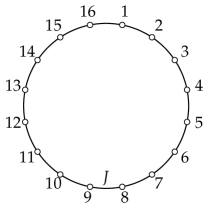
Figure 1: Schematic of the one-dimensional Heisenberg model with $N=16$ sites under the periodic-boundary conditions. The exchange interaction $J$ acts between nearest-neighboring sites at which spin-1/2 spins (i.e., qubits) reside.

III Spatial symmetries

In this section, we first briefly review the projection operator that can restore the Hamiltonian symmetry of an arbitrary quantum state. The projection operator is composed of a set of symmetry operations that do not alter the Hamiltonian. We then discuss how to implement these symmetry operations on a quantum circuit.

III.1 Projection operator and symmetrized state

In general, a quantum many-body system possesses its own particular symmetry and the Hamiltonian describing such a quantum many-body system is invariant under a set of symmetry operations that define the symmetry. These symmetry operations form a group, the Hamiltonian symmetry group, and the symmetry that is relevant to our study here is spatial symmetry such as point group symmetry and translational symmetry of a lattice where the order of the group is finite. It is well known that an irreducible representation of any finite group can be chosen to be unitary Inui et al. (1990).

The projection operator for the $l$th basis ($l=1,\dots,d_{\gamma}$) of an irreducible representation $\gamma$ in a finite group $\mathcal{G}$ is given by

$$\hat{P}^{(\gamma)}_{l}=\frac{d_{\gamma}}{|\mathcal{G}|}\sum_{\hat{g}\in\mathcal{G}}\left[{\bar{D}}^{(\gamma)}(\hat{g})\right]^{*}_{ll}\hat{g},$$ (5)

where $d_{\gamma}$ is the dimension of the irreducible representation $\gamma$, $|\mathcal{G}|$ is the order of $\mathcal{G}$, $\hat{g}$ is a symmetry (unitary) operation in the group $\mathcal{G}$, and $\left[{\bar{D}}^{(\gamma)}(\hat{g})\right]_{ll}$ is the $l$th diagonal element of a matrix representation for the symmetry operation $\hat{g}$ in the irreducible representation $\gamma$ Inui et al. (1990); PJO . Here, $\hat{g}$ satisfies $\hat{g}\hat{\mathcal{H}}\hat{g}^{-1}=\hat{\mathcal{H}}$, or equivalently $[\hat{\mathcal{H}},\hat{g}]=0$. Thus the projection operator commutes with the Hamiltonian,

$$\left[\hat{\mathcal{H}},\hat{P}^{(\gamma)}_{l}\right]=0.$$ (6)

Note also that the projection operator is idempotent $(\hat{P}^{(\gamma)}_{l})^{2}=\hat{P}^{(\gamma)}_{l}$ and Hermitian $(\hat{P}^{(\gamma)}_{l})^{\dagger}=\hat{P}^{(\gamma)}_{l}$, but not unitary. Eigenvalues of $\hat{P}^{(\gamma)}_{l}$ are either $0$ or $1$, implying that it is positive semidefinite.

For an arbitrary quantum state $|\psi\rangle$, the symmetry-projected state $\hat{P}^{(\gamma)}_{l}|\psi\rangle$ is indeed the $l$th basis of the irreducible representation $\gamma$ because, for a unitary operator $\hat{g}\in\mathcal{G}$,

$$\hat{g}|\psi^{(\gamma)}_{l}\rangle = \hat{g}\frac{d_{\gamma}}{|\mathcal{G}|}\sum_{\hat{g}^{\prime}\in\mathcal{G}}\left[{\bar{D}}^{(\gamma)}(\hat{g}^{\prime})\right]^{*}_{ll}\hat{g}^{\prime}|\psi^{(\gamma)}_{l}\rangle$$ (7)

$$= \frac{d_{\gamma}}{|\mathcal{G}|}\sum_{\hat{g}^{\prime\prime}\in\mathcal{G}}\left[{\bar{D}}^{(\gamma)}(\hat{g}^{-1}\hat{g}^{\prime\prime})\right]^{*}_{ll}\hat{g}^{\prime\prime}|\psi^{(\gamma)}_{l}\rangle$$

$$= \frac{d_{\gamma}}{|\mathcal{G}|}\sum_{k}\sum_{\hat{g}^{\prime\prime}\in\mathcal{G}}\left[{\bar{D}}^{(\gamma)}(\hat{g}^{-1})\right]^{*}_{lk}\left[{\bar{D}}^{(\gamma)}(\hat{g}^{\prime\prime})\right]^{*}_{kl}\hat{g}^{\prime\prime}|\psi^{(\gamma)}_{l}\rangle$$

$$= \sum_{k}\left[{\bar{D}}^{(\gamma)}(\hat{g})\right]_{kl}|\psi^{(\gamma)}_{k}\rangle,$$

where

$$|\psi^{(\gamma)}_{l}\rangle=\frac{\hat{P}^{(\gamma)}_{l}|\psi\rangle}{\sqrt{\langle\psi|\hat{P}^{(\gamma)}_{l}|\psi\rangle}}.$$ (8)

is the symmetry-projected normalized state, referred to simply as a symmetrized state hereafter, and we used $(\hat{P}^{(\gamma)}_{l})^{2}=\hat{P}^{(\gamma)}_{l}$ in the first line and

$$|\psi^{(\gamma)}_{k}\rangle=\frac{d_{\gamma}}{|\mathcal{G}|}\sum_{\hat{g}\in\mathcal{G}}\left[{\bar{D}}^{(\gamma)}(\hat{g})\right]^{*}_{kl}\hat{g}|\psi^{(\gamma)}_{l}\rangle$$ (9)

in the fourth line, which is proved by using the great orthogonality theorem Inui et al. (1990).

In a one-dimensional representation ($d_{\gamma}=1$), which includes all representations of an Abelian group such as the translation group and the identity representation of any point group, the projection operator defined in Eq. (5) is simply given as

$$\hat{P}^{(\gamma)}=\frac{1}{|\mathcal{G}|}\sum_{\hat{g}\in\mathcal{G}}\chi^{(\gamma)}(\hat{g})^{*}\hat{g},$$ (10)

where $\chi^{(\gamma)}(\hat{g})$ is the character (i.e., the diagonal element of a matrix representation) for the symmetry operation $\hat{g}$ in the irreducible representation $\gamma$ and we omit the subscript “$l$” in $\hat{P}^{(\gamma)}_{l}$. In this case, the symmetry-projected state $\hat{P}^{(\gamma)}|\psi\rangle$ for an arbitrary quantum state $|\psi\rangle$ is an eigenstate of a unitary operator $\hat{g}\in\mathcal{G}$ with eigenvalue $\chi^{(\gamma)}(\hat{g})$:

$$\hat{g}\left(\hat{P}^{(\gamma)}|\psi\rangle\right)=\chi^{(\gamma)}(\hat{g})\left(\hat{P}^{(\gamma)}|\psi\rangle\right).$$ (11)

III.2 Examples of symmetry operations on a quantum circuit

Translational symmetry of a lattice is described by an appropriate space group $\mathcal{G}$. A symmetry operation $\hat{g}\in\mathcal{G}$ can be expressed as a product of SWAP operations, because $\hat{g}$ simply represents a permutation of local (one-qubit) states, and any permutation can be expressed as a product of transpositions.

As examples of $\hat{g}$, Figs. 2(a), 2(b), and 2(c) show translation operations $\hat{T}$, $\hat{T}^{2}$, and $\hat{T}^{3}$, on a six-site ring, respectively. Here, $\hat{T}$ is the one-lattice-space translation such that $\hat{T}|a\rangle_{1}|b\rangle_{2}|c\rangle_{3}|d\rangle_{4}|e\rangle_{5}|f\rangle_{6}=|f\rangle_{1}|a\rangle_{2}|b\rangle_{3}|c\rangle_{4}|d\rangle_{5}|e\rangle_{6}$. Figure 2(a) shows that $\hat{T}$ can be expressed as a product of the SWAP operators as $\hat{T}=\hat{\mathcal{P}}_{12}\hat{\mathcal{P}}_{23}\hat{\mathcal{P}}_{34}\hat{\mathcal{P}}_{45}\hat{\mathcal{P}}_{56}$. Naively, one can obtain the one-dimensional $n$-lattice-space translation $\hat{T}^{n}$ by repeatedly applying the set of the gates of the elementary translation $\hat{T}$ for $n$ times ($n$: integer). However, the representation of a given permutation in terms of a product of transpositions is not unique and such a construction of $\hat{T}^{n}$ may not be optimal with respect to the number of the SWAP gates. The gates shown in Figs. 2(b) and 2(c) are simplified ones for $\hat{T}^{2}$ and $\hat{T}^{3}$, respectively, by allowing long-range SWAP gates. Note that $\hat{T}^{4}=(\hat{T}^{2})^{-1}$ and $\hat{T}^{5}=\hat{T}^{-1}$ can be obtained by reversing the order of SWAP operations in Figs. 2(b) and 2(a), respectively.

Figure 2: Examples of symmetry operations on a six-qubit system for (a) one-qubit translation $\hat{T}$, (b) two-qubit translation $\hat{T}^{2}$, and (c) three-qubit translation $\hat{T}^{3}$.

III.3 General implementation of symmetry operations on a quantum circuit

As a way of implementing generic permutations, one can make use of the “Amida lottery” (sometime also known as “ghost leg” or “ladder climbing”) construction. Figure 3 illustrates how to construct a desired permutation with nearest-neighbor SWAP operations. Here, the qubits are depicted as vertical lines and the time evolves forward from top to bottom, to be compatible with the conventional two-line notation of a permutation, such as, for example,

$$\mathcal{S}\equiv\left(\begin{matrix}a&b&c&d&e&f\\ e&f&a&b&c&d\\ \end{matrix}\right).$$ (12)

Figure 3(a) is an oracle $\hat{g}$ which performs the permutation $\mathcal{S}$ on one-qubit states,

$$\hat{g}|a\rangle_{1}|b\rangle_{2}|c\rangle_{3}|d\rangle_{4}|e\rangle_{5}|f\rangle_{6}=|e\rangle_{1}|f\rangle_{2}|a\rangle_{3}|b\rangle_{4}|c\rangle_{5}|d\rangle_{6}.$$ (13)

The oracle can be implemented as a product of nearest-neighbor-SWAP operations shown in Fig. 3(b). The circuit structure in Fig. 3(b) can be obtained with the following procedure [see Fig. 3(c)]: (i) draw (unwinding) lines connecting the same one-qubit states in the initial and the final states, (ii) find all the vertices of the lines drawn, and (iii) replace every vertex and its associated four lines, respectively, with a SWAP gate and two vertically aligned lines connected by the SWAP gate (see inset of Fig. 3).

Three remarks are in order. First, drawing winding or zigzag lines in the procedure (i) can produce the same permutation, but the resulting circuit may contain unnecessary SWAP operations. Second, one can further modify the obtained circuit structure by introducing long-range SWAP gates. Third, the inverse permutation, corresponding to $\hat{g}^{\dagger}=\hat{g}^{-1}$, can be obtained merely by inverting the diagram.

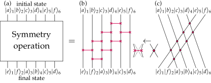
Figure 3: An illustration of the “Amida lottery” construction to implement a general permutation with nearest-neighbor SWAP operations. (a) An oracle of a desired symmetry operation (permutation). (b) A realization of the oracle in (a) with nearest-neighbor SWAP operations. The SWAP gates are highlighted with red thick lines. (c) The same one-qubit states in the initial and the final states are connected by the straight line. The vertices are highlighted with red circles. The vertical lines in panels (a) and (b) represent qubits, while the lines in panel (c) are auxiliary. The inset describes how each vertex in panel (c) is replaced with a SWAP gate in panel (b).

IV Symmetry-adapted VQE method

In this section, we first introduce a spin-symmetric quantum state that generally breaks spatial symmetry. This is a fundamental step to prepare a spin-singlet state. Next we describe the symmetry-adapted VQE scheme. The procedure is essentially the same as the conventional VQE scheme Peruzzo et al. (2014); McClean et al. (2016); Kandala et al. (2017) except that the nonunitary projection operator, applied onto a quantum state that is described by a parametrized quantum circuit, is treated on classical computers when the variational parameters are updated for the next iteration. To optimize the variational parameters, we employ the NGD method, which requires the energy gradient and the metric tensor. We derive these quantities analytically for a symmetrized variational quantum state by taking into account the fact that the symmetrized state is not normalized because the projection operator is not unitary. Once the variational parameters in the parametrized quantum circuit are optimized, the expectation values of quantities, including those other than the Hamiltonian, for the symmetrized state can be evaluated using the resulting circuit by treating the nonunitary projection operator on classical computers as postprocessing.

IV.1 Spin-symmetric trial state

The total-spin squared operator ${\hat{\boldsymbol{S}}}^{2}$ and the total magnetization operator $\hat{S}_{z}$ are defined, respectively, as $\hat{\boldsymbol{S}}^{2}=\frac{1}{4}\sum_{i=1}^{N}\sum_{j=1}^{N}\left(\hat{X}_{i}\hat{X}_{j}+\hat{Y}_{i}\hat{Y}_{j}+\hat{Z}_{i}\hat{Z}_{j}\right)$ and $\hat{S}_{z}=\frac{1}{2}\sum_{i=1}^{N}\hat{Z}_{i}$. Since $[\hat{\mathcal{H}},\hat{\boldsymbol{S}}^{2}]=0$ and $[\hat{\mathcal{H}},\hat{S}_{z}]=0$, any eigenstate $|\Psi_{n}\rangle$ of $\hat{\mathcal{H}}$ is a simultaneous eigenstate of $\hat{\boldsymbol{S}}^{2}$ and $\hat{S}_{z}$, i.e.,

$$\hat{\mathcal{H}}|\Psi_{n}\rangle = E_{n}|\Psi_{n}\rangle,$$ (14)

$$\hat{\boldsymbol{S}}^{2}|\Psi_{n}\rangle = S(S+1)|\Psi_{n}\rangle,$$ (15)

$$\hat{S}_{z}|\Psi_{n}\rangle = S_{z}|\Psi_{n}\rangle,$$ (16)

where $n\,(=0,\ldots,2^{N}-1)$ labels the eigenstates of $\hat{\mathcal{H}}$, and $E_{n}$, $S(S+1)$, and $S_{z}$ are the eigenvalues of $\hat{\mathcal{H}}$, $\hat{\boldsymbol{S}}^{2}$, and $\hat{S}_{z}$, respectively. Without loss of generality, we assume that $E_{0}\leqslant E_{1}\leqslant\ldots\leqslant E_{2^{N}-1}$. The ground state and the ground-state energy of $\hat{\mathcal{H}}$ are thus denoted by $|\Psi_{0}\rangle$ and $E_{0}$, respectively.

It can be shown that the ground state of the Heisenberg model is in the subspace of $S=0$ Lieb and Mattis (1962). To construct a variational state within this subspace, we first prepare a singlet-pair product state

$$|\Phi\rangle=\bigotimes_{i=1}^{N/2}|s_{2i-1,2i}\rangle,$$ (17)

where $|s_{i,j}\rangle=(|0\rangle_{i}|1\rangle_{j}-|1\rangle_{i}|0\rangle_{j})/\sqrt{2}$ is the spin-singlet state (i.e., one of the Bell states) formed between the $i$th and $j$th qubits, and therefore $|\Phi\rangle$ is spin singlet. Then we apply exponential SWAP (eSWAP) gates Loss and DiVincenzo (1998); DiVincenzo et al. (2000); Brunner et al. (2011); Lloyd et al. (2014); Lau and Plenio (2016), each of which is equivalent to the SWAP^α gate up to a two-qubit global phase factor Fan et al. (2005); Balakrishnan and Sankaranarayanan (2008), and preserves the spin SU(2) symmetry Gard et al. (2020); Liu et al. (2019). The eSWAP gates are parametrized by a set of angles $\boldsymbol{\theta}$ to evolve the state from $|\Phi\rangle$ to (an approximation of) the true ground state $|\Psi_{0}\rangle$, while keeping the state in the subspace of $S=0$ during the evolution.

The unitary operator $U_{ij}(\theta)$ corresponding to the eSWAP gate acting on two qubits $i$ and $j$ with a parameter $\theta$ is given by

$$\hat{U}_{ij}(\theta) \equiv \exp(-{\rm i}\theta\hat{\mathcal{P}}_{ij}/2)$$ (18)

$$= \hat{I}\cos{\frac{\theta}{2}}-{\rm i}\hat{\mathcal{P}}_{ij}\sin{\frac{\theta}{2}},$$

where the involutority of the SWAP operator $\hat{\mathcal{P}}_{ij}^{2}=\hat{I}$ is used. A decomposition of the eSWAP gate in terms of more elementary gates is described in Appendix A. By writing the sequence of the eSWAP operations as

$$\hat{\mathcal{U}}(\boldsymbol{\theta})=\prod_{\langle i,j\rangle}\hat{U}_{ij}(\theta_{ij}),$$ (19)

with the order of multiplications specified in the circuit construction (see Fig. 4), our trial wavefunction is given by

$$|\Psi(\boldsymbol{\theta})\rangle=\hat{\mathcal{U}}(\boldsymbol{\theta})|\Phi\rangle.$$ (20)

Note that $|\Psi(\boldsymbol{\theta})\rangle$ preserves the spin symmetry of the Hamiltonian but not the spatial symmetry, as apparently seen in Fig. 4. The order of multiplication of the eSWAP gates in the circuit shown in Fig. 4 is motivated by an adiabatic evolution of the state from the initial state $|\Phi\rangle$ to the (approximate) ground state of $\hat{\cal H}$ in Eq. (1) Ho and Hsieh (2019). A physical interpretation of the trial wavefunction $|\Psi(\boldsymbol{\theta})\rangle$ in conjunction with a resonating-valence-bond (RVB) state Pauling (1933); Anderson (1973); Fazekas and Anderson (1974), a superposition of a great number of singlet-pair product states Oguchi and Kitatani (1989), known as one of the best variational states to describe quantum many-body states Becca and Sorella (2017), is discussed in Appendix B. Note that, as shown in Appendix C, a spin-singlet pair formed by qubits that are separated even at the largest distance can be generated in $|\Psi(\boldsymbol{\theta})\rangle$ with $D\sim N/4$, where $D$ is the number of layers, each layer being composed of $N$ eSWAP gates (see Fig. 4).

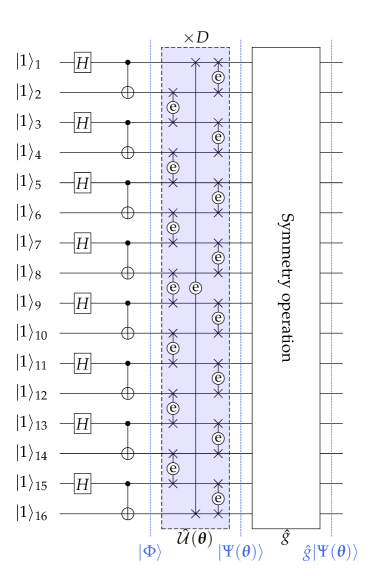
Figure 4: The circuit structure that generates a state $\hat{g}|\Psi(\boldsymbol{\theta})\rangle=\hat{g}\hat{\mathcal{U}}(\boldsymbol{\theta})|\Phi\rangle$. The symmetry operation $\hat{g}$ can be implemented according to the scheme described in Sec. III.3. The circuit consists of $N$ qubits ($N=16$ in the figure) with $D$ layers of gates, each layer being composed of $N$ eSWAP gates (indicated by shaded blue), and the symmetry operation gates. Here, the eSWAP gate is represented by the SWAP gate with symbol “e”. Since each eSWAP gate contains a single variational parameter, there exist $N\times D$ variational parameters to be optimized in the circuit.

IV.2 Energy expectation value

Although $|\Psi(\boldsymbol{\theta})\rangle$ is symmetric in the spin space, generally it breaks the spatial symmetry of Hamiltonian because of a particular structure of the circuit. As described in Sec. III.1, we apply the projection operator ${\hat{P}}^{(\gamma)}$ to symmetrize $|\Psi(\boldsymbol{\theta})\rangle$ not . The resulting symmetrized variational state with the irreducible representation $\gamma$ is

$$|\Psi^{(\gamma)}(\boldsymbol{\theta})\rangle=\frac{\hat{P}^{(\gamma)}}{\sqrt{\mathcal{N}(\boldsymbol{\theta})}}|\Psi(\boldsymbol{\theta})\rangle,$$ (21)

where

$$\mathcal{N}(\boldsymbol{\theta})=\langle\Psi(\boldsymbol{\theta})|\hat{P}^{(\gamma)}|\Psi(\boldsymbol{\theta})\rangle.$$ (22)

Note that $\mathcal{N}(\boldsymbol{\theta})\geqslant 0$ because the projection operator $\hat{P}^{(\gamma)}$ is a positive semidefinite operator. The corresponding variational energy is given by

$$E^{(\gamma)}(\boldsymbol{\theta}) \equiv E[\Psi^{(\gamma)}(\boldsymbol{\theta})]$$ (23)

$$\equiv \langle\Psi^{(\gamma)}(\boldsymbol{\theta})|\hat{\mathcal{H}}|\Psi^{(\gamma)}(\boldsymbol{\theta})\rangle$$

$$= \frac{\langle\Psi(\boldsymbol{\theta})|\hat{\mathcal{H}}\hat{P}^{(\gamma)}|\Psi(\boldsymbol{\theta})\rangle}{\langle\Psi(\boldsymbol{\theta})|\hat{P}^{(\gamma)}|\Psi(\boldsymbol{\theta})\rangle}$$

$$= \frac{\sum_{\hat{g}\in\mathcal{G}}\chi^{(\gamma)}(\hat{g})^{*}\langle\Psi(\boldsymbol{\theta})|\hat{\mathcal{H}}\hat{g}|\Psi(\boldsymbol{\theta})\rangle}{\sum_{\hat{g}\in\mathcal{G}}\chi^{(\gamma)}(\hat{g})^{*}\langle\Psi(\boldsymbol{\theta})|\hat{g}|\Psi(\boldsymbol{\theta})\rangle}.$$

In the symmetry-adapted VQE scheme, the matrix elements in the numerator and the denominator in Eq. (23) are evaluated on quantum computers by, for example, introducing one ancilla qubit Li and Benjamin (2017); Romero et al. (2018); Mitarai and Fujii (2019); Dallaire-Demers et al. (2019). This can be done efficiently because $\hat{\mathcal{H}}$ is a sum of unitary operators and $\hat{g}$ is a unitary operator as well. The sum over the group operations $\hat{g}$, the order of $\mathcal{G}$ being $\mathcal{O}(N)$, is performed on classical computers as postprocessing AV .

It should be noted that the linear combination of unitary operators can also be implemented with a circuit described in, e.g., Ref. Childs and Weibe (2012). The advantage of such a circuit is that it can generate the symmetrized state $\hat{P}^{(\gamma)}|\Psi(\boldsymbol{\theta})\rangle$ directly without introducing the postprocessing. However, one major disadvantage of such a circuit, particularly in the current NISQ era, is that the circuit structure becomes much more complicated than the one proposed here because it requires $\log_{2}|\mathcal{G}|$ ancilla qubits and $|\mathcal{G}|$ controlled-unitary operations, in addition to the gates necessary to describe $|\Psi(\boldsymbol{\theta})\rangle$ shown in Fig. 4.

IV.3 Natural-gradient-descent optimization

The variational parameters $\boldsymbol{\theta}$ are optimized by minimizing $E^{(\gamma)}(\boldsymbol{\theta})$ with the NGD optimization Amari (1998). Starting from chosen (e.g., random) initial parameters $\boldsymbol{\theta}_{1}$, the NGD optimization at the $k$th iteration updates the variational parameters as

$$\boldsymbol{\theta}_{k+1}=\boldsymbol{\theta}_{k}-\alpha\left[{\rm Re}\boldsymbol{G}^{(\gamma)}(\boldsymbol{\theta}_{k})\right]^{-1}\boldsymbol{\nabla}E^{(\gamma)}(\boldsymbol{\theta}_{k}),$$ (24)

where $\alpha$ is a parameter for tuning the step width (i.e., a learning rate) and

$$[\boldsymbol{G}^{(\gamma)}(\boldsymbol{\theta})]_{ij} \equiv \left[\boldsymbol{G}[\Psi^{(\gamma)}(\boldsymbol{\theta})]\right]_{ij}$$ (25)

$$= \langle\partial_{\theta_{i}}\Psi^{(\gamma)}(\boldsymbol{\theta})|\partial_{\theta_{j}}\Psi^{(\gamma)}(\boldsymbol{\theta})\rangle$$

$$- \langle\partial_{\theta_{i}}\Psi^{(\gamma)}(\boldsymbol{\theta})|\Psi^{(\gamma)}(\boldsymbol{\theta})\rangle\langle\Psi^{(\gamma)}(\boldsymbol{\theta})|\partial_{\theta_{j}}\Psi^{(\gamma)}(\boldsymbol{\theta})\rangle$$

is the metric tensor Provost and Vallee (1980) of the variational-parameter ($\boldsymbol{\theta}$) space associated with the normalized state $|\Psi^{(\gamma)}(\boldsymbol{\theta})\rangle$. Since $\boldsymbol{G}^{(\gamma)}(\boldsymbol{\theta})$ is positive semidefinite, $\alpha$ has to be chosen positive to minimize the variational energy. In the numerical simulations shown in Sec. V, we set $\alpha=0.1/J$.

We should note that essentially the same optimization scheme, which takes into account the geometry of the wavefunction in the variational parameter space, has been introduced as the stochastic-reconfiguration method and applied successfully with the variational Monte Carlo technique for correlated electron systems Sorella (2001); Casula and Sorella (2003); Yunoki and Sorella (2006). An equivalence between the stochastic-reconfiguration method and the real- and imaginary-time evolution of a variational state has been pointed out Carleo et al. (2012, 2014); Ido et al. (2015); Takai et al. (2016); Nomura et al. (2017). On the other hand, very recently, as a optimization method, the imaginary-time evolution of a variational quantum state has been proposed in the context of VQE approach Endo et al. (b); McArdle et al. (2019b); Jones et al. (2019). This method was later recognized to be essentially the same as the NGD optimization of a parametrized quantum circuit Stokes et al. ; Yamamoto .

IV.4 Energy gradient and metric tensor

The energy gradient $\boldsymbol{\nabla}E^{(\gamma)}(\boldsymbol{\theta})$ in Eq. (24) and the metric tensor $\boldsymbol{G}^{(\gamma)}(\boldsymbol{\theta})$ in Eq. (25) are now expressed in terms of the circuit (non-symmetrized) state $|\Psi(\boldsymbol{\theta})\rangle$ and its derivative $|\partial_{\theta_{i}}\Psi(\boldsymbol{\theta})\rangle$. For this purpose, first we can readily show that the derivative of the symmetrized state, $|\partial_{\theta_{i}}\Psi^{(\gamma)}(\boldsymbol{\theta})\rangle$, can be expressed as

$$|\partial_{\theta_{i}}\Psi^{(\gamma)}(\boldsymbol{\theta})\rangle = \frac{\hat{P}^{(\gamma)}}{\sqrt{\mathcal{N}(\boldsymbol{\theta})}}\left[|\partial_{\theta_{i}}\Psi(\boldsymbol{\theta})\rangle-{\rm Re}\mathcal{A}_{i}(\boldsymbol{\theta})|\Psi(\boldsymbol{\theta})\rangle\right]$$ (26)

with

$$\mathcal{A}_{i}(\boldsymbol{\theta}) = \frac{\langle\Psi(\boldsymbol{\theta})|\hat{P}^{(\gamma)}|\partial_{\theta_{i}}\Psi(\boldsymbol{\theta})\rangle}{\mathcal{N}(\boldsymbol{\theta})}.$$ (27)

Note that the real part of $\mathcal{A}_{i}(\boldsymbol{\theta})$ is related to the logarithmic derivative of the norm:

$$\partial_{\theta_{i}}\ln\mathcal{N}(\boldsymbol{\theta})=2{\rm Re}\mathcal{A}_{i}(\boldsymbol{\theta}),$$ (28)

and the imaginary part of $\mathcal{A}_{i}(\boldsymbol{\theta})$ is related to the Berry connection:

$$\langle\Psi^{(\gamma)}(\boldsymbol{\theta})|\partial_{\theta_{i}}\Psi^{(\gamma)}(\boldsymbol{\theta})\rangle=\mathcal{A}_{i}(\boldsymbol{\theta})-{\rm Re}\mathcal{A}_{i}(\boldsymbol{\theta})={\rm i}{\rm Im}\mathcal{A}_{i}(\boldsymbol{\theta}).$$ (29)

From Eq. (26), the derivative of the variational energy $E^{(\gamma)}(\boldsymbol{\theta})$ can be expressed as

$$\partial_{\theta_{i}}E^{(\gamma)}(\boldsymbol{\theta})=2{\rm Re}\left[\frac{\langle\Psi(\boldsymbol{\theta})|\hat{P}^{(\gamma)}\hat{\mathcal{H}}|\partial_{\theta_{i}}\Psi(\boldsymbol{\theta})\rangle}{\mathcal{N}(\boldsymbol{\theta})}-\mathcal{A}_{i}(\boldsymbol{\theta})E^{(\gamma)}(\boldsymbol{\theta})\right].$$ (30)

Similarly, by substituting Eq. (26) into Eq. (25), we can show that the metric tensor $[\boldsymbol{G}^{(\gamma)}(\boldsymbol{\theta})]_{ij}$ is now given as

$$[\boldsymbol{G}^{(\gamma)}(\boldsymbol{\theta})]_{ij} = \frac{\langle\partial_{\theta_{i}}\Psi(\boldsymbol{\theta})|\hat{P}^{(\gamma)}|\partial_{\theta_{j}}\Psi(\boldsymbol{\theta})\rangle}{\mathcal{N}(\boldsymbol{\theta})}-\mathcal{A}_{i}^{*}(\boldsymbol{\theta})\mathcal{A}_{j}(\boldsymbol{\theta}).$$ (31)

Note that Eqs. (26), (27), (30), and (31) are generic form for the state subject to the symmetry-projection operator.

For numerical simulations, to evaluate the derivatives of the trial state, we employ the parameter-shift rule for the (non-symmetrized) state

$$|\partial_{\theta_{i}}\Psi(\boldsymbol{\theta})\rangle=\frac{1}{2}|\Psi(\boldsymbol{\theta}+\pi\boldsymbol{e}_{i})\rangle,$$ (32)

which readily follows from Eq. (18). Here, $\boldsymbol{e}_{i}$ is the unit vector whose $i^{\prime}$th entry is given by $[\boldsymbol{e}_{i}]_{i^{\prime}}=\delta_{ii^{\prime}}$. We should also note that our numerical simulations in the next section employ the NGD optimization because, as described above, this optimization method has been repeatedly proved to be currently the best method for optimizing a variational wavefunction with many variational parameters in the variational Monte Carlo technique for quantum many-body systems, when up to the first order derivative of the variational energy is available Becca and Sorella (2017). If we employ this optimization method in the real experiment, we have to evaluate, in addition to the matrix elements in the numerator and the denominator in Eq. (23), several other quantities appearing in Eqs. (30) and (31) on quantum computers. However, the use of the NGD optimization is not necessarily required in the symmetry-adapted VQE scheme and we can always adopt a simpler optimization method without even using the first derivative of the variational energy.

V Results

Here we demonstrate the symmetry-adapted VQE approach by numerically simulating the spin-1/2 Heisenberg ring.

V.1 Ground-state energy

Figures 5 and 6 show a typical behavior of the fidelity and the variational energy $E^{(\gamma)}(\boldsymbol{\theta}_{k})$, respectively, for $N=16$ as a function of the NGD iteration $k$ in Eq. (24). Here, we use the translational symmetry of the Hamiltonian that forms the cyclic group $\mathcal{G}=\{\hat{T}^{1},\hat{T}^{2},\ldots,\hat{T}^{N}\}$ with $|\mathcal{G}|=N$. The character associated with the operation $\hat{T}^{n}$ is given by

$$\chi^{(q)}(\hat{T}^{n})={\rm e}^{{\rm i}qn},$$ (33)

where $q=2\pi m/N$ with $m=-N/2+1,-N/2+2,\ldots,N/2-1,N/2$, corresponding to the total momentum of the symmetrized state, and the dimension $d_{q}$ of the representation $q$ is $1$. The ground state of the spin-1/2 Heisenberg ring for $N=16$ is at the $q=0$ sector and spin singlet.

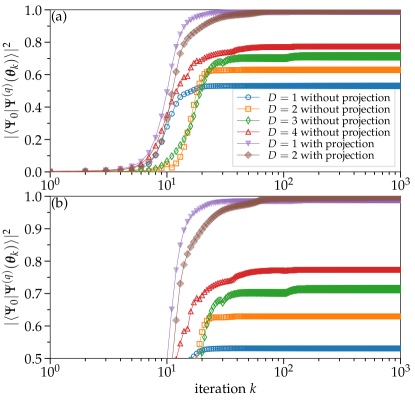
Figure 5: Semi-log plot of the fidelity $\left|\langle\Psi_{0}|\Psi^{(q)}(\bm{\theta}_{k})\rangle\right|^{2}$ of the ground state for the spin-1/2 Heisenberg ring with $N=16$ as a function of the NGD iteration $k$ in Eq. (24). The results with different number of layers ($D$), and with (filled symbols) and without (empty symbols) use of the translational symmetry, are shown. (b) Enlarged figure of panel (a). $|\Psi_{0}\rangle$ is the exact ground state and $|\Psi^{(q)}(\bm{\theta}_{k})\rangle$ is an approximate ground state obtained after the $k$th iteration of optimizing the variational parameters in the circuit. The number of total variational parameters is $N\times D$. The initial parameters $\boldsymbol{\theta}_{1}$ are set randomly and we use the same initial parameters $\boldsymbol{\theta}_{1}$ for all the simulations shown here when $D$ is the same.

Figure 5 shows the fidelity $F\equiv\left|\langle\Psi_{0}|\Psi^{(q)}(\bm{\theta}_{k})\rangle\right|^{2}$ of the ground state between the exact ground state $|\Psi_{0}\rangle$, calculated with the Lanczos exact diagonalization method Lin (1990); Dagotto (1994); Weiße and Fehske (2008), and the approximate ground state $|\Psi^{(q)}(\bm{\theta}_{k})\rangle$ obtained after the $k$th iteration of optimizing the variational parameters in the circuit with different layer depths $D$. For comparison, the results for the cases with the same circuit structure but not symmetrized are also shown. The fidelity $F$ for both symmetrized and non-symmetrized cases is less than $1\%$ when $k=1$ and rapidly increases at $k\approx 10$. However, the fidelity $F$ is significantly worse for the non-symmetrized cases, even when $D=4$, corresponding to the circuit with $N\times D=64$ variational parameters. In sharp contrast, when the symmetry is imposed, the fidelity $F$ becomes as large as $98.8\%$ already for the shallowest circuit with $D=1$ and $99.9\%$ with $D=2$, clearly demonstrating an excellent improvement by symmetrizing the state.

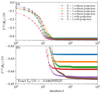
Figure 6: Same as Fig. 5 but for the variational energy of the ground state. The horizontal line in (b) indicates the exact ground-state energy $E_{0}$.

Figure 6 shows the variational energy of the ground state calculated using $|\Psi^{(q)}(\bm{\theta}_{k})\rangle$ for both symmetrized and non-symmetrized cases with different layer depth $D$ in the circuit. As a reference, the exact ground-state energy $E_{0}$ calculated with the Lanczos exact diagonalization method is also shown. As expected from the fidelity results in Fig. 5, the converged variational energy $E^{(q)}(\bm{\theta}_{k})$ for the non-symmetrized cases is much larger than the exact value $E_{0}$ even when $D=4$. On the other hand, the symmetrized case can obtain the decently accurate energy already for $D=1$ because $E^{(q)}(\bm{\theta}_{k=10^{3}})/JN=-0.4447$. The variational energy is further improved by increasing the number of layers to $D=2$, in which $E^{(q)}(\bm{\theta}_{k=10^{3}})/JN=-0.4461$ is essentially exact.

V.2 Excitation energy

One of the advantages of the symmetry-adapted VQE scheme is that it can resolve the quantum numbers of the eigenstates simply by using the character $\chi^{(q)}(\hat{T}^{n})$ of the desired quantum number $q$. Here we demonstrate this for the lowest magnetically excited states by calculating the variational energy in the $S=1$ sector at momentum $q$,

$$E_{S=1}^{(q)}(\boldsymbol{\theta})\equiv E[\tilde{\Psi}^{(q)}(\boldsymbol{\theta})]=\frac{\langle\tilde{\Psi}(\boldsymbol{\theta})|\hat{\mathcal{H}}\hat{P}^{(q)}|\tilde{\Psi}(\boldsymbol{\theta})\rangle}{\langle\tilde{\Psi}(\boldsymbol{\theta})|\hat{P}^{(q)}|\tilde{\Psi}(\boldsymbol{\theta})\rangle},$$ (34)

where $|\tilde{\Psi}(\boldsymbol{\theta})\rangle=\hat{\mathcal{U}}(\boldsymbol{\theta})|\tilde{\Phi}\rangle$ with

$$|\tilde{\Phi}\rangle=\bigotimes_{i=1}^{N/2-1}|s_{2i-1,2i}\rangle|t_{N-1,N}\rangle$$ (35)

and $|t_{ij}\rangle=(|0\rangle_{i}|1\rangle_{j}+|1\rangle_{i}|0\rangle_{j})/{\sqrt{2}}$. Note that $|\tilde{\Phi}\rangle$ has the quantum numbers $S=1$ and $S_{z}=0$ Oguchi and Kitatani (1989) and therefore $|\tilde{\Psi}(\boldsymbol{\theta})\rangle$ also preserves these quantum numbers. The quantum state $|\tilde{\Psi}(\boldsymbol{\theta})\rangle$ can be generated from the same circuit structure in Fig. 4 merely by setting the initial state at, for example, the $15$th qubit to $|0\rangle_{15}$, instead of $|1\rangle_{15}$ (see also Appendix B). Notice also that varying the values of $q$ does not require any change in the circuit structure, because momentum $q$ enters only in the character $\chi^{(q)}(\hat{T}^{n})$ [see Eq. (23)]. Thus, the circuit structure for the excited-state calculation remains the same as that for the ground-state calculation.

Figure 7 shows the spin-triplet excitation energy,

$$\Delta E\equiv E^{(q)}_{S=1}(\tilde{\boldsymbol{\theta}}^{*})-E^{(0)}(\boldsymbol{\theta}^{*}),$$ (36)

for different momentum $q$, where $E^{(0)}(\boldsymbol{\theta}^{*})$ is the variational energy of the ground state discussed in Sec. V.1 and $E^{(q)}_{S=1}(\tilde{\boldsymbol{\theta}}^{*})$ is the variational energy at the $S=1$ sector with momentum $q$ given in Eq. (34). $\tilde{\boldsymbol{\theta}}^{*}$ and $\boldsymbol{\theta}^{*}$ are the optimized variational parameters by minimizing separately the corresponding energy functional, for which we take the values at the $k=1000$th iteration. As shown in Fig. 7, the calculated excitation energies agree well with the exact results already for the shallowest circuit with $D=1$. Moreover, with increasing the number of layers to $D=2$, the accuracy improves systematically, as in the ground-state-energy calculations. These results demonstrate that the symmetry-adapted VQE scheme can also be used to approximate low-lying excited states.

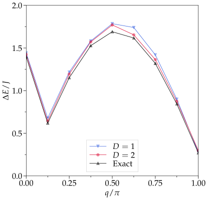
Figure 7: Momentum-resolved spin-triplet ($S=1$) excitations for the spin-1/2 Heisenberg ring with $N=16$. The excitation energy $\Delta E$ is calculated as the difference of the variational energies for the excited state with $S=1$ and momentum $q$ and the ground state. $D$ is the number of layers in the circuit (see Fig. 4). For comparison, the exact results are also shown.

VI Conclusions and discussions

We have proposed a scheme to adapt the Hamiltonian symmetry in the hybrid quantum-classical VQE approach. The proposed scheme is to make use of the projection operator $\hat{P}^{(\gamma)}_{l}$ to project a quantum state, which is described by a quantum circuit that usually breaks the Hamiltonian symmetry in the VQE approach, onto the $l$th basis of the irreducible representation $\gamma$ of the Hamiltonian symmetry group $\mathcal{G}$. In the symmetry-adapted VQE scheme proposed here, the nonunitarity of the projection operator is treated as postprocessing on classical computers. We have also introduced the “Amida lottery” construction to implement general symmetry operations in quantum circuits. Here, each symmetry operation $\hat{g}$ is simply represented as a different product of $O(N)$ SWAP operations and therefore $|\mathcal{G}|$ different circuits are required in the symmetry-adapted VQE scheme.

Although the symmetry-adapted VQE scheme introduced here is probably the simplest and most direct way to implement the Hamiltonian symmetry in the VQE framework, our numerical simulations for the spin-1/2 Heisenberg ring clearly demonstrated that the improvement is significant in terms of both the fidelity of the ground state and the ground-state energy by showing that the circuit with the shallowest layer already achieves the decent accuracy. Moreover, we have demonstrated that the symmetry-adapted VQE scheme, combined with the spin-quantum-number-projected circuit state, allows us to compute, for example, the spin-triplet excitation energies as a function of momentum.

Recently, a VQE approach with a Jastrow-type operator, which is an exponential of a Hermitian operator and is nonunitary in general, has been implemented using a quantum hardware Mazzola et al. (2019). While the symmetry projection operator $\hat{P}^{(\gamma)}_{l}$ is also Hermitian and nonunitary, it is much simpler than the Jastrow-type operator, in the sense that $\hat{P}^{(\gamma)}_{l}$ is idempotent and composed of the finite number $|\mathcal{G}|$ of unitary operators. In addition, $\hat{P}^{(\gamma)}_{l}$ commutes with $\hat{\mathcal{H}}$, which simplifies the evaluation of the variational energy, as in Eq. (23), and its derivative with respect to a variational parameter. We thus expect that the symmetry-adapted VQE approach described here can be implemented soon with a quantum hardware (also see Appendix D). To this end, an efficient experimental implementation of SWAP operations is highly desirable to perform symmetry operations.

Appendix A Decomposition of eSWAP gate

A decomposition of the eSWAP gate to elementary gates is given in Fig. 8. Here, $\hat{R}_{X}(\theta)=\exp(-{\rm i}\theta\hat{X}/2)$ and $R_{-\theta/2}$ is the phase-shift gate that acts on a qubit as $\hat{R}_{-\theta/2}|0\rangle_{i}=|0\rangle_{i}$ and $\hat{R}_{-\theta/2}|1\rangle_{i}={\rm e}^{-{\rm i}\theta/2}|1\rangle_{i}$. The decomposition in Fig. 8 can be confirmed readily in the matrix representation as

$$\begin{bmatrix}{\rm e}^{-{\rm i}\theta/2}&0&0&0\\ 0&\cos\frac{\theta}{2}&-{\rm i}\sin{\frac{\theta}{2}}&0\\ 0&-{\rm i}\sin\frac{\theta}{2}&\cos{\frac{\theta}{2}}&0\\ 0&0&0&{\rm e}^{-{\rm i}\theta/2}\\ \end{bmatrix}$$ (37)

$$= \begin{bmatrix}1&0&0&0\\ 0&0&0&1\\ 0&0&1&0\\ 0&1&0&0\\ \end{bmatrix}\begin{bmatrix}0&0&1&0\\ 0&0&0&1\\ 1&0&0&0\\ 0&1&0&0\\ \end{bmatrix}\begin{bmatrix}1&0&0&0\\ 0&1&0&0\\ 0&0&{\rm e}^{-{\rm i}\theta/2}\\ 0&0&0&{\rm e}^{-{\rm i}\theta/2}\\ \end{bmatrix}\begin{bmatrix}0&0&1&0\\ 0&0&0&1\\ 1&0&0&0\\ 0&1&0&0\\ \end{bmatrix}$$

$$\times \begin{bmatrix}1&0&0&0\\ 0&1&0&0\\ 0&0&\cos\frac{\theta}{2}&-{\rm i}\sin{\frac{\theta}{2}}\\ 0&0&-{\rm i}\sin\frac{\theta}{2}&\cos{\frac{\theta}{2}}\\ \end{bmatrix}\begin{bmatrix}1&0&0&0\\ 0&0&0&1\\ 0&0&1&0\\ 0&1&0&0\\ \end{bmatrix},$$

where the matrix in the left-hand side represents the eSWAP gate itself [see Eq. (18)], and the matrices in the right-hand side represent controlled-NOT (CNOT), controlled-$R_{X}$, $X\otimes I$, $R_{-\theta/2}\otimes I$, $X\otimes I$, and CNOT gates, respectively, from right to left in Eq. (37). Here, the matrices are represented with respect to the conventional two-qubit basis states $|0\rangle_{i}|0\rangle_{j}$, $|0\rangle_{i}|1\rangle_{j}$, $|1\rangle_{i}|0\rangle_{j}$, and $|1\rangle_{i}|1\rangle_{j}$. If necessary, the controlled-$R_{X}$ gate can be further decomposed into elementary gates Barenco et al. (1995). From the matrix representation on the left-hand side of Eq. (37), it is obvious that the eSWAP gate is equivalent to the ${\rm SWAP}^{\alpha}$ gate up to a phase factor Fan et al. (2005); Balakrishnan and Sankaranarayanan (2008).

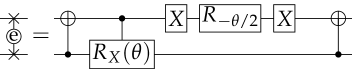
Figure 8: A decomposition of the eSWAP gate that is parametrized with $\theta$.

Appendix B RVB-type state on a quantum circuit

For a physical interpretation of $|\Psi(\boldsymbol{\theta})\rangle=\hat{\mathcal{U}}(\boldsymbol{\theta})|\Phi\rangle$ (see Fig. 4), it is important to understand how the SWAP and eSWAP gates act on the singlet-pair product state $|\Phi\rangle$. First, it should be noticed that ${\hat{\mathcal{P}}}_{ij}$ alters the sign of the wavefunction if it is operated on the singlet state $|s_{ij}\rangle$ formed between qubits $i$ and $j$:

$${\hat{\mathcal{P}}}_{ij}|s_{ij}\rangle=|s_{ji}\rangle=-|s_{ij}\rangle.$$ (38)

This is simply because the singlet state is antisymmetric with respect to the permutation of $i$ and $j$. In other words, $|s_{ij}\rangle$ is an eigenstate of ${\hat{\mathcal{P}}}_{ij}$ with eigenvalue $-1$. The corresponding eSWAP operation results in

$${\hat{U}_{ij}(\theta)}|s_{ij}\rangle={\rm e}^{{\rm i}\theta/2}|s_{ij}\rangle.$$ (39)

Thus, $|s_{ij}\rangle$ is an eigenstate of ${\hat{U}_{ij}(\theta)}$ and operating ${\hat{U}_{ij}(\theta)}$ is equivalent to multiplying a phase factor on $|s_{ij}\rangle$.

If a SWAP gate is operated between two qubits, each of them contributing separately to form different singlets, then it recombines the singlet pairs as

$${\hat{\mathcal{P}}}_{jk}|s_{ij}\rangle|s_{kl}\rangle=|s_{ik}\rangle|s_{jl}\rangle.$$ (40)

Note that the resulting singlet pairs are not necessarily formed between the adjacent qubits (see for example Refs. Kivelson et al. (1987); Affleck et al. (1988); Tasaki and Kohmoto (1990)). The corresponding eSWAP operation results in

$${\hat{U}_{jk}(\theta)}|s_{ij}\rangle|s_{kl}\rangle=\cos{\frac{\theta}{2}}|s_{ij}\rangle|s_{kl}\rangle-{\rm i}\sin{\frac{\theta}{2}}|s_{ik}\rangle|s_{jl}\rangle.$$ (41)

A crucial feature of the eSWAP gate is that it not only recombines two singlet pairs but also superposes two singlet-pair product states with parametrized amplitudes. Namely, the resulting state is a superposition of the original singlet pairs and those generated by the SWAP operation, which is essential to generate an RVB state from the reference singlet-pair product state $|\Phi\rangle$, as will be discussed below. Indeed, Eq. (41) can already explain how an RVB state can be generated on a four qubit system (see Fig. 9). Notice that the state represented by the crossed diagram such as the one in Fig. 9 can be expressed as a linear combination of those represented by non-crossed diagrams Saito (1990).

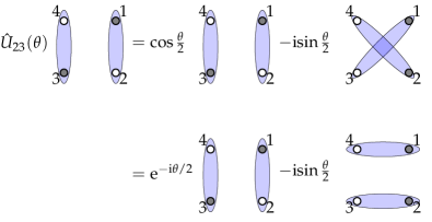
Figure 9: A schematic figure of the eSWAP operation on a four qubit system. An ellipse enclosing two circles (solid and open circles) represents a singlet-pair state with the sign convention that, for example, the singlet-pair state formed by qubits 1 and 2 in the left most side, indicated by solid and open circles, respectively, is $|s_{1,2}\rangle=(|0\rangle_{1}|1\rangle_{2}-|1\rangle_{1}|0\rangle_{2})/\sqrt{2}$. The eSWAP operation between the qubits 2 and 3 results in a superposition of the different singlet-pair product states, i.e., an RVB state.

The reference state $|\Phi\rangle$ used here is a dimerized state where the singlet pairs are located on the links between adjacent qubits $(1,2),\,(3,4),\,\ldots,\,(N-1,N)$. Such a state breaks the translational symmetry. A repeated application of the eSWAP gates, implemented in $\hat{\mathcal{U}}(\boldsymbol{\theta})$, on $|\Phi\rangle$ generates a large number of different dimer coverings (configurations of spin-singlet pairs covering all qubits) $\mathcal{C}[\Psi(\boldsymbol{\theta})]$, composed of both short-range and long-range singlet pairs LR- , which are superposed in the circuit with coefficients parametrized by $\boldsymbol{\theta}$. Thus $|\Psi(\boldsymbol{\theta})\rangle$ might be able to restore the translational symmetry that is broken in $|\Phi\rangle$, if the number $D$ of layers is large enough. The present symmetry-adapted VQE scheme, instead, restores the spatial symmetry by applying the projection operator on $|\Psi(\boldsymbol{\theta})\rangle$.

The trial state generated by the circuit that is used in the present study thus has a form

$$|\Psi(\boldsymbol{\theta})\rangle=\sum_{\mathcal{C}[\Psi(\boldsymbol{\theta})]}w(\mathcal{C}[\Psi(\boldsymbol{\theta})])\bigotimes_{[i,j]\in\mathcal{C}[\Psi(\boldsymbol{\theta})]}|s_{ij}\rangle,$$ (42)

where $[i,j]$ denotes a pair of two qubits that form $|s_{ij}\rangle$, ${\mathcal{C}[\Psi(\boldsymbol{\theta})]}$ indicates all possible dimer coverings generated on a given circuit, and $w(\mathcal{C}[\Psi(\boldsymbol{\theta})])$ is a coefficient for a singlet-pair product state specified by a configuration ${\mathcal{C}[\Psi(\boldsymbol{\theta})]}$. It is now obvious that this state in Eq. (42) has a form of the RVB state

$$|{\rm RVB}\rangle=\sum_{\mathcal{C}}w(\mathcal{C})\bigotimes_{[i,j]\in\mathcal{C}}|s_{ij}\rangle,$$ (43)

where ${\mathcal{C}}$ denotes all possible dimer coverings and $w(\mathcal{C})$ is the corresponding coefficient. For example, if $w(\mathcal{C})$ is taken to be equally weighted for all the configurations that consist of only nearest-neighbor singlet pairs, $|{\rm RVB}\rangle$ reduces to a so-called short-range RVB state (see for example Ref. Yunoki and Sorella (2006) for a detailed description). However, we should emphasize the important difference between $|\Psi(\boldsymbol{\theta})\rangle$ and $|{\rm RVB}\rangle$. While all the coefficients $w(\mathcal{C})$ in $|{\rm RVB}\rangle$ can be set independently for different realizations of all possible dimer coverings ${\mathcal{C}}$, the coefficients $w(\mathcal{C}[\Psi(\boldsymbol{\theta})])$ in $|\Psi(\boldsymbol{\theta})\rangle$ are not independent but related to each other via the variational parameters $\bm{\theta}$ in the circuit even though the repeated application of the eSWAP gates can eventually produce all possible dimer coverings.

The RVB state has often been used as a variational wavefunction for approximating the ground states of the spin-1/2 Heisenberg model in square Liang et al. (1988); Poilblanc (1989), triangular Oguchi et al. (1986), and kagome lattices Sindzingre et al. (1994). A numerical study on small clusters up to 26 spins Nakagawa et al. (1990) has shown that, by taking into account the Marshall’s sign rule Marshall (1955), the RVB state with only a few variational parameters can accurately represent the ground state of the spin-1/2 Heisenberg model in a square lattice, and that the (long-range) RVB state substantially improves the variational energy and the variational state as compared to the short-range RVB state.

Finally, we briefly note on calculations in higher spin-quantum-number sectors assuming that $N$ is even. One can derive relations similar to Eqs. (38)–(41) for the spin-triplet states $|t_{ij}\rangle\equiv(|0\rangle_{i}|1\rangle_{j}+|1\rangle_{i}|0\rangle_{j})/\sqrt{2}$, $|t_{ij}^{+}\rangle\equiv|0\rangle_{i}|0\rangle_{j}$, and $|t_{ij}^{-}\rangle\equiv|1\rangle_{i}|1\rangle_{j}$. A difference here from the case of $|s_{ij}\rangle$ is that the triplet states are symmetric under the SWAP operation. By using a product state of $N/2-1$ singlet pairs and a single triplet pair $|t_{ij}\rangle$, instead of $|\Phi\rangle$, as the reference state, one can search for the lowest-energy state within the subspace of $S=1$ and $S_{z}=0$, as demonstrated in Sec. V.2 (see Ref. Oguchi and Kitatani (1989) for a detailed analysis). The calculation in the higher $S$ sectors with finite-$S_{z}$ states is also possible simply by using $|t^{+}_{ij}\rangle$ or $|t^{-}_{ij}\rangle$ for the reference state. Finding the lowest energy in the higher spin sectors is useful for studying, for example, whether a magnetic long-range order exists in the thermodynamic limit from finite-size calculations Bernu et al. (1994); Sindzingre et al. (2002); Sindzingre (2004); Shannon et al. (2006).

Such a circuit explicitly specifies the subspace labeled by the spin-quantum numbers $S$ and $S_{z}$, and thus is specialized to spin-isotropic (i.e., SU(2) symmetric) Heisenberg models. On classical computers, with a sophisticated and elaborated algorithm that incorporates the spatial symmetry, such as the lattice translational symmetry, and $S_{z}$ conservation Lin (1990); Weiße (2013), one can obtain the numerically exact ground state of the spin-1/2 Heisenberg model up to $50$ spins Wietek and Läuchli (2018), which is far larger than the case of $16$ qubits studied here. However, $\boldsymbol{S}^{2}$ conservation is usually not implemented because the programming of a total-spin-preserved code is, although possible Bostrem et al. (2006); Heitmann and Schnack (2019), not easy and often computationally demanding on classical computers. We expect that the circuit that operates eSWAP gates on a singlet-pair product state or on a pair-product state with higher spin-quantum numbers might be useful for studying spin-liquid states including the RVB state as well as excited states on quantum computers in the near future. Regarding excitations and dynamics, we should also note that the eSWAP operations naturally appear also in such simulations when a Suzuki-Trotter decomposition is applied to the time-evolution operator ${\rm e}^{-{\rm i}\hat{\mathcal{H}}t}$ with $t$ being time Suzuki (1976); Trotter (1959).

Appendix C Generation of spin-singlet pairs formed by distant qubits

In this Appendix, we show that a spin-singlet pair formed by qubits that are separated at the largest distance can still be generated by repeated application of the nearest-neighbor eSWAP gates on the singlet-pair product state $|\Phi\rangle$ with $D~{}\sim N/4$ for the one-dimensional chain of $N$ qubits under the periodic boundary conditions.

Let us first consider how a spin-singlet state with $r$-lattice spacing, e.g.,

$$|s_{1,1+r}\rangle,$$ (44)

can be generated from the singlet-pair product state $|\Phi\rangle$. Here, to be specific, we assume that $N$ and $r$ are both even. According to Eq. (40), a long-range SWAP operation $\hat{\mathcal{P}}_{2,r+1}$ on two nearest-neighbor spin-singlet pairs $|s_{1,2}\rangle$ and $|s_{r+1,r+2}\rangle$ generates such $r$-distant singlet pairs:

$$\mathcal{\hat{P}}_{2,r+1}|s_{1,2}\rangle|s_{r+1,r+2}\rangle=|s_{1,r+1}\rangle|s_{2,r+2}\rangle.$$ (45)

Figure 10 illustrates the generation of spin-singlet pairs formed by distant qubits in the case of $N=16$ and $r=8$.

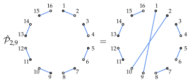
Figure 10: Schematic figure of a long-range SWAP operation on the singlet-pair product state $|\Phi\rangle$ for $N=16$ and $r=8$. Here a singlet-pair state is represented by a blue line ending with solid and open circles.

Next, we consider how the long-range SWAP operator $\hat{\mathcal{P}}_{2,r+1}$ can be represented as a product of the nearest-neighbor SWAP operators. For this purpose, we make use of the “Amida lottery” construction introduced in Sec. III.3. Figure 11 shows that, following the “Amida lottery” construction, the long-range SWAP operation can indeed be expressed as a product of the nearest-neighbor SWAP operations that form an X-like shape on the circuit. The number $N_{\rm SWAP}(r)$ of the nearest-neighbor SWAP gates necessary in the circuit is

$$N_{\rm SWAP}(r)=2(r-2)+1=2r-3,$$ (46)

as there are $r-2$ qubits between the $2$nd and $(r+1)$st qubits (see Fig. 11). One can also find that, with this construction, the depth of the circuit or the number of “time steps” $\tau_{\rm SWAP}(r)$ required is

$$\tau_{\rm SWAP}(r)=(r-2)+1=r-1.$$ (47)

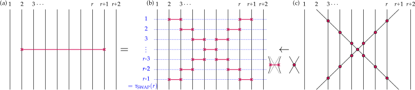
Figure 11: A decomposition of a long-range SWAP gate with the “Amida lottery” construction. (a) The long-range SWAP gate $\hat{\mathcal{P}}_{2,r+1}$ with $r=8$. (b) A decomposition of $\hat{\mathcal{P}}_{2,r+1}$ to the nearest-neighbor SWAP gates. The horizontal dashed lines associated with the numbers $1,2,\cdots,\tau_{\rm SWAP}(r)=r-1$ indicate the time steps. (c) Auxiliary figure that generates the decomposition of the long-range SWAP gate into the nearest-neighbor SWAP gates shown in (b).

Noticing that $\hat{U}_{ij}(0)=\hat{I}$ and $\hat{U}_{ij}(\pm\pi)=\mp{\rm i}\hat{\mathcal{P}}_{ij}$ in Eqs. (18) and (19), we can now readily show that the sequence $\hat{\mathcal{U}}(\boldsymbol{\theta})$ of the nearest-neighbor eSWAP operations in Fig. 4 with a particular set of parameters $\boldsymbol{\theta}=\boldsymbol{\theta}_{\rm SWAP}$ can produce $\hat{\mathcal{P}}_{2,r+1}$, up to a global phase factor, i.e.,

$$\hat{\mathcal{U}}(\boldsymbol{\theta}_{\rm SWAP})=\pm{\rm i}\hat{\mathcal{P}}_{2,r+1}.$$ (48)

Namely, $\boldsymbol{\theta}_{\rm SWAP}$ has $\theta_{ij}=\pm\pi$ if $\langle i,j\rangle$ corresponds to the link on which the nearest-neighbor SWAP operation is required for $\hat{\mathcal{P}}_{2,r+1}$, and $\theta_{ij}=0$, otherwise (see Fig. 12). The global phase factor, which is however irrelevant for the purpose of this Appendix, in Eq. (48) appears because $N_{\rm SWAP}(r)$ is odd, and depends on how the sign of $\theta_{ij}=\pm\pi$ is chosen. The number $D(r)$ of layers in $\hat{\mathcal{U}}(\boldsymbol{\theta}_{\rm SWAP})$ required for producing $\hat{\mathcal{P}}_{2,r+1}$ is thus

$$D(r)=\left\lceil\frac{\tau_{\rm SWAP}(r)}{2}\right\rceil=\left\lceil\frac{r}{2}-\frac{1}{2}\right\rceil,$$ (49)

where $\lceil\cdot\rceil$ denotes the ceiling function which returns the minimum integer larger than or equal to the argument. The argument in Eq. (49) is divided by $2$ because each layer of $\hat{\mathcal{U}}(\boldsymbol{\theta})$ contains two time steps (see Fig. 12).

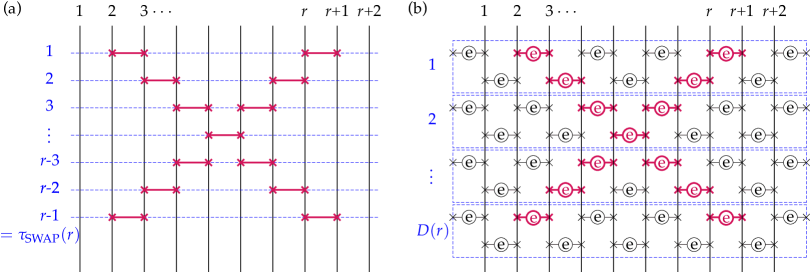
Figure 12: (a) The long-range SWAP gate $\hat{\mathcal{P}}_{2,r+1}$ with $r=8$ generated by a set of the nearest-neighbor SWAP gates (see Fig. 11). (b) An equivalent operation (up to a global phase factor) can be described by the sequence $\hat{\mathcal{U}}(\boldsymbol{\theta}_{\rm SWAP})$ of the nearest-neighbor eSWAP gates, where the rotation angles $\theta_{ij}$ are either $\pi$ or $-\pi$ for the eSWAP gates highlighted with red thick lines, and $\theta_{ij}=0$, otherwise. Each dashed box associated with the number $1,2,\cdots$, or $D(r)$ in (b) corresponds to the single layer of the parametrized gates indicated by shaded blue in Fig. 4.

Under the periodic-boundary condition, the largest distance $r_{\rm max}$ is

$$r_{\rm max}=N/2.$$ (50)

Therefore, to generate a spin-singlet pair formed by qubits separated at the largest distance, the required number of layers is

$$D(r_{\rm max})=\left\lceil\frac{N}{4}-\frac{1}{2}\right\rceil,$$ (51)

i.e., $D(r_{\rm max})\sim N/4$. However, this does not necessarily imply that all possible dimer coverings are generated with $D=D(r_{\rm max})$.

Finally, we note that since $\boldsymbol{\theta}$ in general takes arbitrary values, $|\Psi(\boldsymbol{\theta})\rangle=\hat{\mathcal{U}}(\boldsymbol{\theta})|\Phi\rangle$ is a superposition of many different singlet-product states represented by different dimer coverings, among which spin-singlet pairs formed by distant qubits are certainly contained, as discussed above, although only the nearest-neighbor eSWAP gates are applied in the circuit.

Appendix D Simulation on quantum hardware

To validate the relevance of the RVB-type wavefunction as a trial wavefunction on quantum computers, in this Appendix we estimate the ground state energy for a small system ($N=4$) using the ibmqx2 chip, which consists of five qubits, available through an online quantum computing network provided by IBM (IBM Q 5 Yorktown) IBM with the Qiskit python API for programming the device Abraham et al. (2019).

Let us first review the ground-state properties of the spin-$1/2$ Heisenberg model on the $N=4$ ring. With the labeling of qubits shown in Fig. 9, the exact ground state $|\Psi_{0}\rangle$ is given by

$$|\Psi_{0}\rangle=\frac{1}{\sqrt{3}}\left(|s_{1,2}\rangle|s_{3,4}\rangle+|s_{4,1}\rangle|s_{2,3}\rangle\right).$$ (52)

$|\Psi_{0}\rangle$ is a superposition of the two singlet-pair product states with the same probability amplitude, and is correctly normalized because these singlet-pair product states are not orthogonal to each other but have an overlap of $(\langle s_{4,1}|\langle s_{2,3}|)(|s_{1,2}\rangle|s_{3,4}\rangle)=1/2$. The corresponding exact ground-state energy is

$$E_{0}=-2J.$$ (53)

In terms of the expectation value of the Hamiltonian, $E_{0}$ is expressed as

$$E_{0}=\frac{J}{4}\sum_{i=1}^{N}\langle\Psi_{0}|\left(\hat{X}_{i}\hat{X}_{i+1}+\hat{Y}_{i}\hat{Y}_{i+1}+\hat{Z}_{i}\hat{Z}_{i+1}\right)|\Psi_{0}\rangle,$$ (54)

where $i+1$ should be identified as $1$ if $i=N$ because of the periodic-boundary conditions. Since $|\Psi_{0}\rangle$ is spin-symmetric and translationally invariant, Eq. (53) can be rephrased in terms of the exact nearest-neighbor spin correlation functions as

$$\langle\Psi_{0}|\hat{X}_{i}\hat{X}_{i+1}|\Psi_{0}\rangle=\langle\Psi_{0}|\hat{Y}_{i}\hat{Y}_{i+1}|\Psi_{0}\rangle=\langle\Psi_{0}|\hat{Z}_{i}\hat{Z}_{i+1}|\Psi_{0}\rangle$$

$$= \frac{E_{0}}{3N(J/4)}=-\frac{2}{3}$$ (55)

for any $i$.

Next we show that, up to a global phase factor, $|\Psi_{0}\rangle$ can be produced by applying two eSWAP gates on the singlet-pair product state $|s_{1,2}\rangle|s_{3,4}\rangle$. A straightforward calculation with Eqs. (39) and (41) shows that

$$\hat{U}_{34}(\theta_{2})\hat{U}_{23}(\theta_{1})|s_{1,2}\rangle|s_{3,4}\rangle={\rm e}^{{\rm i}\phi}|\Psi_{0}\rangle,$$ (56)

where

$${\theta_{1}}=2\arccos{\left(-\sqrt{\frac{2}{3}}\right)}=1.6081734479693928\times\pi,$$ (57)

$${\theta_{2}}=2\arccos{\left(-\sqrt{\frac{1}{3}}\right)}=1.3918265520306072\times\pi,$$ (58)

and ${\rm e}^{{\rm i}\phi}=\sqrt{\frac{2}{3}}-\sqrt{\frac{1}{3}}{\rm i}$. Hereafter, we ignore the global phase factor ${\rm e}^{{\rm i}\phi}$ because it is irrelevant for the energy estimation.

Now we consider the energy estimation on quantum computers. Equation (55) implies that evaluating one of these correlation functions suffices for estimating $E_{0}$. Here, we evaluate the correlation function $\langle\Psi_{0}|\hat{X}_{1}\hat{X}_{2}|\Psi_{0}\rangle$ by using the Hadamard test as

$${\rm Re}\langle\Psi_{0}|\hat{X}_{1}\hat{X}_{2}|\Psi_{0}\rangle=p_{0}-p_{1},$$ (59)

where

$$p_{0} =\frac{1}{2}\left(1+{\rm Re}\langle\Psi_{0}|\hat{X}_{1}\hat{X}_{2}|\Psi_{0}\rangle\right)$$ (60)

and

$$p_{1} =\frac{1}{2}\left(1-{\rm Re}\langle\Psi_{0}|\hat{X}_{1}\hat{X}_{2}|\Psi_{0}\rangle\right)$$ (61)

are probabilities of observing $0$ and $1$, respectively, by measuring out the ancilla ($0$th) qubit in Fig. 13 DM . Among the correlation functions, $\hat{X}_{1}\hat{X}_{2}$ is chosen because CNOT gate is implemented as one of the basis gates on the ibmqx2 chip. Moreover, since $\hat{X}_{1}\hat{X}_{2}$ does not involve qubits $3$ and $4$, operation of $\hat{U}_{34}(\theta_{2})$ is not necessary for measurements of $\hat{X}_{1}\hat{X}_{2}$. Namely, since $\left[\hat{X}_{1}\hat{X}_{2},\hat{U}_{34}(\theta)\right]=0$ for any $\theta$, the correlation function can be simplified as

$$\langle\Psi_{0}|\hat{X}_{1}\hat{X}_{2}|\Psi_{0}\rangle =\langle\tilde{\Psi}_{0}|\hat{U}_{34}(\theta_{2})^{\dagger}\hat{X}_{1}\hat{X}_{2}\hat{U}_{34}(\theta_{2})|\tilde{\Psi}_{0}\rangle$$

$$=\langle\tilde{\Psi}_{0}|\hat{X}_{1}\hat{X}_{2}|\tilde{\Psi}_{0}\rangle,$$ (62)

where

$$|\tilde{\Psi}_{0}\rangle=\hat{U}_{23}(\theta_{1})|s_{1,2}\rangle|s_{3,4}\rangle.$$ (63)

On the ibmqx2 chip, we implement a circuit that generates $|\tilde{\Psi}_{0}\rangle$ for measurements. The eSWAP gate corresponding to $\hat{U}_{23}(\theta_{1})$ is implemented with the decomposition shown in Fig. 8, where the controlled-$R_{X}$ gate is further decomposed in the way described in Ref. Barenco et al. (1995).

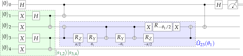
Figure 13: The circuit used for evaluating ${\rm Re}\langle\Psi_{0}|\hat{X}_{1}\hat{X}_{2}|\Psi_{0}\rangle={\rm Re}\langle\tilde{\Psi}_{0}|\hat{X}_{1}\hat{X}_{2}|\tilde{\Psi}_{0}\rangle$ on the ibmqx2 chip. The state $|\tilde{\Psi}_{0}\rangle=\hat{U}_{23}(\theta_{1})|s_{1,2}\rangle|s_{3,4}\rangle$ is generated on the first to fourth qubits. The parts of the circuit corresponding to $|s_{1,2}\rangle|s_{3,4}\rangle$ and $\hat{U}_{23}(\theta_{1})$ are highlighted with shaded green and blue boxes, respectively. The rotation angles for $R_{Y}$ and $R_{Z}$ gates are also indicated below these gates.

Table 1 shows the probabilities $p_{0}$ and $p_{1}$, and estimated values of ${\rm Re}\langle\Psi_{0}|\hat{X}_{1}\hat{X}_{2}|\Psi_{0}\rangle$ from 16 samples, each of which consists of 1024 measurements. The negative values of ${\rm Re}\langle\Psi_{0}|\hat{X}_{1}\hat{X}_{2}|\Psi_{0}\rangle$ imply the antiferromagnetic correlation between the nearest-neighbor spins. In the ideal (noiseless) case, the probabilities are $p_{0}=1/6$ and $p_{1}=5/6$. Averaging over the results of the 16 samples yields ${\rm Re}\langle\Psi_{0}|\hat{X}_{1}\hat{X}_{2}|\Psi_{0}\rangle=-0.66894(549)$ and hence $E_{0}/J=-2.00682(1647)$, where the numbers in parentheses represent the standard error of the mean for the last digits. Therefore, the exact energy is obtained within the statistical error.

Table 1: Probabilities $p_{0}$ and $p_{1}$ obtained from quantum simulations on the ibmqx2 chip. The values on each row are obtained from 1024 measurements. Ideal (noiseless) results are also shown in the bottom row. Data were obtained on 6 April 2020 (EST) DAT .

Sample	$p_{0}(\%)$	$p_{1}(\%)$	${\rm Re}\langle\Psi_{0}|\hat{X}_{1}\hat{X}_{2}|\Psi_{0}\rangle$
1	15.430	84.570	-0.69140
2	17.969	82.031	-0.64062
3	15.625	84.375	-0.68750
4	16.309	83.691	-0.67382
5	16.016	83.984	-0.67968
6	15.430	84.570	-0.69140
7	17.578	82.422	-0.64844
8	18.457	81.543	-0.63086
9	17.090	82.910	-0.65820
10	17.969	82.031	-0.64062
11	16.602	83.398	-0.66796
12	17.090	82.910	-0.65820
13	16.992	83.008	-0.66016
14	15.527	84.473	-0.68946
15	16.113	83.887	-0.67774
16	14.648	85.352	-0.70704
Mean	16.553(274)	83.447(274)	-0.66894(549)
Ideal	16.667	83.333	-0.66667

It is interesting to note that the ground-state energy obtained here is significantly better than the one estimated with the hardware-efficient ansatz reported in Ref. Kandala et al. (2017), where the ground-state energy is approximately $-1.5J$ H_I . The substantial improvement found here over the circuit based on the hardware-efficient ansatz is highly instructive and suggests that the construction of quantum circuits based on the RVB-type wavefunction, which takes into account the spin rotational symmetry, is a better strategy to describe the ground state (and also excited states) of the Heisenberg model on quantum computers.

Finally, we comment on quantum simulations of the same system with the symmetry-projection scheme. Unfortunately, we have found it difficult to implement the symmetry operators on a real quantum device at present. The difficulty is due to controlled-SWAP (Fredkin) gates, each of which is decomposed into many CNOT gates and one-qubit rotations, causing formidably noisy results. An efficient implementation of the controlled-SWAP (Fredkin) gate in a quantum device, as demonstrated in Ref. Patel et al. (2016), is thus highly desirable.

References

- Nakamura et al. (1999) Y. Nakamura, Y. A. Pashkin, and J. S. Tsai, Nature 398, 786 (1999).
- Kok et al. (2007) P. Kok, W. J. Munro, K. Nemoto, T. C. Ralph, J. P. Dowling, and G. J. Milburn, Rev. Mod. Phys. 79, 135 (2007).
- Ladd et al. (2010) T. D. Ladd, F. Jelezko, R. Laflamme, Y. Nakamura, C. Monroe, and J. L. O’Brien, Nature 464, 45 (2010).
- Xiang et al. (2013) Z.-L. Xiang, S. Ashhab, J. Q. You, and F. Nori, Rev. Mod. Phys. 85, 623 (2013).
- Chow et al. (2014) J. M. Chow, J. M. Gambetta, E. Magesan, D. W. Abraham, A. W. Cross, B. R. Johnson, N. A. Masluk, C. A. Ryan, J. A. Smolin, S. J. Srinivasan, and M. Steffen, Nature Communications 5, 4015 (2014).
- Barends et al. (2014) R. Barends, J. Kelly, A. Megrant, A. Veitia, D. Sank, E. Jeffrey, T. C. White, J. Mutus, A. G. Fowler, B. Campbell, Y. Chen, Z. Chen, B. Chiaro, A. Dunsworth, C. Neill, P. O’Malley, P. Roushan, A. Vainsencher, J. Wenner, A. N. Korotkov, A. N. Cleland, and J. M. Martinis, Nature 508, 500 EP (2014).
- Ristè et al. (2015) D. Ristè, S. Poletto, M.-Z. Huang, A. Bruno, V. Vesterinen, O.-P. Saira, and L. DiCarlo, Nature Communications 6, 6983 (2015).
- Kelly et al. (2015) J. Kelly, R. Barends, A. G. Fowler, A. Megrant, E. Jeffrey, T. C. White, D. Sank, J. Y. Mutus, B. Campbell, Y. Chen, Z. Chen, B. Chiaro, A. Dunsworth, I.-C. Hoi, C. Neill, P. J. J. O’Malley, C. Quintana, P. Roushan, A. Vainsencher, J. Wenner, A. N. Cleland, and J. M. Martinis, Nature 519, 66 EP (2015).
- Arute et al. (2019) F. Arute, K. Arya, R. Babbush, D. Bacon, J. C. Bardin, R. Barends, R. Biswas, S. Boixo, F. G. S. L. Brandao, D. A. Buell, B. Burkett, Y. Chen, Z. Chen, B. Chiaro, R. Collins, W. Courtney, A. Dunsworth, E. Farhi, B. Foxen, A. Fowler, C. Gidney, M. Giustina, R. Graff, K. Guerin, S. Habegger, M. P. Harrigan, M. J. Hartmann, A. Ho, M. Hoffmann, T. Huang, T. S. Humble, S. V. Isakov, E. Jeffrey, Z. Jiang, D. Kafri, K. Kechedzhi, J. Kelly, P. V. Klimov, S. Knysh, A. Korotkov, F. Kostritsa, D. Landhuis, M. Lindmark, E. Lucero, D. Lyakh, S. Mandrà, J. R. McClean, M. McEwen, A. Megrant, X. Mi, K. Michielsen, M. Mohseni, J. Mutus, O. Naaman, M. Neeley, C. Neill, M. Y. Niu, E. Ostby, A. Petukhov, J. C. Platt, C. Quintana, E. G. Rieffel, P. Roushan, N. C. Rubin, D. Sank, K. J. Satzinger, V. Smelyanskiy, K. J. Sung, M. D. Trevithick, A. Vainsencher, B. Villalonga, T. White, Z. J. Yao, P. Yeh, A. Zalcman, H. Neven, and J. M. Martinis, Nature 574, 505 (2019).
- Feynman (1982) R. P. Feynman, International Journal of Theoretical Physics 21, 467 (1982).
- Peruzzo et al. (2014) A. Peruzzo, J. McClean, P. Shadbolt, M.-H. Yung, X.-Q. Zhou, P. J. Love, A. Aspuru-Guzik, and J. L. O’Brien, Nature Communications 5, 4213 (2014).
- McClean et al. (2016) J. R. McClean, J. Romero, R. Babbush, and A. Aspuru-Guzik, New Journal of Physics 18, 023023 (2016).
- Kandala et al. (2017) A. Kandala, A. Mezzacapo, K. Temme, M. Takita, M. Brink, J. M. Chow, and J. M. Gambetta, Nature 549, 242 (2017).
- Preskill (2018) J. Preskill, Quantum 2, 79 (2018).
- Li et al. (2017) J. Li, X. Yang, X. Peng, and C.-P. Sun, Phys. Rev. Lett. 118, 150503 (2017).
- Mitarai et al. (2018) K. Mitarai, M. Negoro, M. Kitagawa, and K. Fujii, Phys. Rev. A 98, 032309 (2018).
- Motta et al. (2019) M. Motta, C. Sun, A. T. K. Tan, M. J. O’Rourke, E. Ye, A. J. Minnich, F. G. S. L. Brandão, and G. K.-L. Chan, Nature Physics 16, 205 (2019).
- (18) K. M. Nakanishi, K. Fujii, and S. Todo, arXiv:1903.12166 [quant-ph] .
- (19) R. M. Parrish, J. T. Iosue, A. Ozaeta, and P. L. McMahon, arXiv:1904.03206 [quant-ph] .
- Nakanishi et al. (2019) K. M. Nakanishi, K. Mitarai, and K. Fujii, Phys. Rev. Research 1, 033062 (2019).
- Higgott et al. (2019) O. Higgott, D. Wang, and S. Brierley, Quantum 3, 156 (2019).
- Chiesa et al. (2019) A. Chiesa, F. Tacchino, M. Grossi, P. Santini, I. Tavernelli, D. Gerace, and S. Carretta, Nature Physics 15, 455 (2019).
- Parrish et al. (2019) R. M. Parrish, E. G. Hohenstein, P. L. McMahon, and T. J. Martínez, Phys. Rev. Lett. 122, 230401 (2019).
- Kosugi and Matsushita (2020) T. Kosugi and Y.-i. Matsushita, Phys. Rev. A 101, 012330 (2020).
- Endo et al. (a) S. Endo, I. Kurata, and Y. O. Nakagawa, (a), arXiv:1909.12250 [quant-ph] .
- (26) I. Rungger, N. Fitzpatrick, H. Chen, C. H. Alderete, H. Apel, A. Cowtan, A. Patterson, D. M. Ramo, Y. Zhu, N. H. Nguyen, E. Grant, S. Chretien, L. Wossnig, N. M. Linke, and R. Duncan, “Dynamical mean field theory algorithm and experiment on quantum computers,” arXiv:1910.04735 [quant-ph] .
- Keen et al. (2020) T. Keen, T. Maier, S. Johnston, and P. Lougovski, Quantum Science and Technology 5, 035001 (2020).
- (28) T. Kosugi and Y. Matsushita, “Charge and spin response functions on a quantum computer: applications to molecules,” arXiv:1911.00293 [quant-ph] .
- Riera et al. (2012) A. Riera, C. Gogolin, and J. Eisert, Phys. Rev. Lett. 108, 080402 (2012).
- Dallaire-Demers and Wilhelm (2016) P.-L. Dallaire-Demers and F. K. Wilhelm, Phys. Rev. A 93, 032303 (2016).
- (31) D. Zhu, S. Johri, N. M. Linke, K. A. Landsman, N. H. Nguyen, C. H. Alderete, A. Y. Matsuura, T. H. Hsieh, and C. Monroe, arXiv:1906.02699 [quant-ph] .
- (32) N. Yoshioka, Y. O. Nakagawa, K. Mitarai, and K. Fujii, arXiv:1908.09836 [quant-ph] .
- Macridin et al. (2018a) A. Macridin, P. Spentzouris, J. Amundson, and R. Harnik, Phys. Rev. Lett. 121, 110504 (2018a).
- Macridin et al. (2018b) A. Macridin, P. Spentzouris, J. Amundson, and R. Harnik, Phys. Rev. A 98, 042312 (2018b).
- Sugisaki et al. (2016) K. Sugisaki, S. Yamamoto, S. Nakazawa, K. Toyota, K. Sato, D. Shiomi, and T. Takui, The Journal of Physical Chemistry A 120, 6459 (2016).
- Sugisaki et al. (2019) K. Sugisaki, S. Yamamoto, S. Nakazawa, K. Toyota, K. Sato, D. Shiomi, and T. Takui, Chemical Physics Letters: X 1, 100002 (2019).
- Liu et al. (2019) J.-G. Liu, Y.-H. Zhang, Y. Wan, and L. Wang, Phys. Rev. Research 1, 023025 (2019).
- Gard et al. (2020) B. T. Gard, L. Zhu, G. S. Barron, N. J. Mayhall, S. E. Economou, and E. Barnes, npj Quantum Information 6, 10 (2020).
- Schmitz and Johri (2020) A. T. Schmitz and S. Johri, npj Quantum Information 6, 2 (2020).
- Bonet-Monroig et al. (2018) X. Bonet-Monroig, R. Sagastizabal, M. Singh, and T. E. O’Brien, Phys. Rev. A 98, 062339 (2018).
- Endo et al. (2019) S. Endo, Q. Zhao, Y. Li, S. Benjamin, and X. Yuan, Phys. Rev. A 99, 012334 (2019).
- McArdle et al. (2019a) S. McArdle, X. Yuan, and S. Benjamin, Phys. Rev. Lett. 122, 180501 (2019a).
- Inui et al. (1990) T. Inui, Y. Tanabe, and Y. Onodera, Group Theory and Its Applications in Physics (Springer, Heidelberg, 1990).
-
(44)
When a matrix representation is not
available, we can use the character of the irreducible
representation for the symmetry operation and introduce
the following projection operator:
which projects an arbitrary quantum state onto a state in the irreducible representation , but in general composed of a sum of the base functions that span the subspace of the irreducible representation Inui et al. (1990). - Lieb and Mattis (1962) E. Lieb and D. Mattis, Journal of Mathematical Physics 3, 749 (1962), https://doi.org/10.1063/1.1724276 .
- Loss and DiVincenzo (1998) D. Loss and D. P. DiVincenzo, Phys. Rev. A 57, 120 (1998).
- DiVincenzo et al. (2000) D. P. DiVincenzo, D. Bacon, J. Kempe, G. Burkard, and K. B. Whaley, Nature 408, 339 (2000).
- Brunner et al. (2011) R. Brunner, Y.-S. Shin, T. Obata, M. Pioro-Ladrière, T. Kubo, K. Yoshida, T. Taniyama, Y. Tokura, and S. Tarucha, Phys. Rev. Lett. 107, 146801 (2011).
- Lloyd et al. (2014) S. Lloyd, M. Mohseni, and P. Rebentrost, Nature Physics 10, 631 (2014).
- Lau and Plenio (2016) H.-K. Lau and M. B. Plenio, Phys. Rev. Lett. 117, 100501 (2016).
- Fan et al. (2005) H. Fan, V. Roychowdhury, and T. Szkopek, Phys. Rev. A 72, 052323 (2005).
- Balakrishnan and Sankaranarayanan (2008) S. Balakrishnan and R. Sankaranarayanan, Phys. Rev. A 78, 052305 (2008).
- Ho and Hsieh (2019) W. W. Ho and T. H. Hsieh, SciPost Phys. 6, 29 (2019).
- Pauling (1933) L. Pauling, The Journal of Chemical Physics 1, 280 (1933).
- Anderson (1973) P. Anderson, Materials Research Bulletin 8, 153 (1973).
- Fazekas and Anderson (1974) P. Fazekas and P. W. Anderson, The Philosophical Magazine: A Journal of Theoretical Experimental and Applied Physics 30, 423 (1974).
- Oguchi and Kitatani (1989) T. Oguchi and H. Kitatani, J. Phys. Soc. Jpn. 58, 1403 (1989).
- Becca and Sorella (2017) F. Becca and S. Sorella, Quantum Monte Carlo Approaches for Correlated Systems (Cambridge University Press, Cambridge, 2017).
- (59) Here, we assume that the irreducible representation is one-dimensional. However, the extension to the case of a higher-dimensional irreducible representation is straightforward by using the projection operator in Eq. (5).
- Li and Benjamin (2017) Y. Li and S. C. Benjamin, Phys. Rev. X 7, 021050 (2017).
- Romero et al. (2018) J. Romero, R. Babbush, J. R. McClean, C. Hempel, P. J. Love, and A. Aspuru-Guzik, Quantum Science and Technology 4, 014008 (2018).
- Mitarai and Fujii (2019) K. Mitarai and K. Fujii, Phys. Rev. Research 1, 013006 (2019).
- Dallaire-Demers et al. (2019) P.-L. Dallaire-Demers, J. Romero, L. Veis, S. Sim, and A. Aspuru-Guzik, Quantum Science and Technology 4, 045005 (2019).
- (64) As long as an operator commutes with , the expectation value of is evaluated similarly as in Eq. (23). However, when this is not the case, the numerator of the corresponding formula for the expectation value is slightly more complex and the computational complexity increases by an additional factor.
- Childs and Weibe (2012) A. M. Childs and N. Weibe, Quantum Information and Computation 12, 901 (2012).
- Amari (1998) S.-I. Amari, Neural Comput. 10, 251 (1998).
- Provost and Vallee (1980) J. P. Provost and G. Vallee, Comm. Math. Phys. 76, 289 (1980).
- Sorella (2001) S. Sorella, Phys. Rev. B 64, 024512 (2001).
- Casula and Sorella (2003) M. Casula and S. Sorella, The Journal of Chemical Physics 119, 6500 (2003).
- Yunoki and Sorella (2006) S. Yunoki and S. Sorella, Phys. Rev. B 74, 014408 (2006).
- Carleo et al. (2012) G. Carleo, F. Becca, M. Schiró, and M. Fabrizio, Scientific Reports 2, 243 (2012).
- Carleo et al. (2014) G. Carleo, F. Becca, L. Sanchez-Palencia, S. Sorella, and M. Fabrizio, Phys. Rev. A 89, 031602 (2014).
- Ido et al. (2015) K. Ido, T. Ohgoe, and M. Imada, Phys. Rev. B 92, 245106 (2015).
- Takai et al. (2016) K. Takai, K. Ido, T. Misawa, Y. Yamaji, and M. Imada, Journal of the Physical Society of Japan 85, 034601 (2016).
- Nomura et al. (2017) Y. Nomura, A. S. Darmawan, Y. Yamaji, and M. Imada, Phys. Rev. B 96, 205152 (2017).
- Endo et al. (b) S. Endo, Y. Li, S. Benjamin, and X. Yuan, “Variational quantum simulation of general processes,” (b), arXiv:1812.08778 [quant-ph] .
- McArdle et al. (2019b) S. McArdle, T. Jones, S. Endo, Y. Li, S. C. Benjamin, and X. Yuan, npj Quantum Information 5, 75 (2019b).
- Jones et al. (2019) T. Jones, S. Endo, S. McArdle, X. Yuan, and S. C. Benjamin, Phys. Rev. A 99, 062304 (2019).
- (79) J. Stokes, J. Izaac, N. Killoran, and G. Carleo, “Quantum natural gradient,” arXiv:1909.02108 [quant-ph] .
- (80) N. Yamamoto, “On the natural gradient for variational quantum eigensolver,” arXiv:1909.05074 [quant-ph] .
- Lin (1990) H. Q. Lin, Phys. Rev. B 42, 6561 (1990).
- Dagotto (1994) E. Dagotto, Rev. Mod. Phys. 66, 763 (1994).
- Weiße and Fehske (2008) A. Weiße and H. Fehske, “Exact diagonalization techniques,” in Computational Many-Particle Physics, Vol. 739, edited by H. Fehske, R. Schneider, and A. Weiße (Springer Berlin Heidelberg, Berlin, Heidelberg, 2008) pp. 529–544.
- Mazzola et al. (2019) G. Mazzola, P. J. Ollitrault, P. K. Barkoutsos, and I. Tavernelli, Phys. Rev. Lett. 123, 130501 (2019).
- Barenco et al. (1995) A. Barenco, C. H. Bennett, R. Cleve, D. P. DiVincenzo, N. Margolus, P. Shor, T. Sleator, J. A. Smolin, and H. Weinfurter, Phys. Rev. A 52, 3457 (1995).
- Kivelson et al. (1987) S. A. Kivelson, D. S. Rokhsar, and J. P. Sethna, Phys. Rev. B 35, 8865 (1987).
- Affleck et al. (1988) I. Affleck, T. Kennedy, E. H. Lieb, and H. Tasaki, Comm. Math. Phys. 115, 477 (1988).
- Tasaki and Kohmoto (1990) H. Tasaki and M. Kohmoto, Phys. Rev. B 42, 2547 (1990).
- Saito (1990) R. Saito, Journal of the Physical Society of Japan 59, 482 (1990), https://doi.org/10.1143/JPSJ.59.482 .
- (90) This is the case even though the eSWAP gates are repeatedly applied only between adjacent qubits, as shown in Fig. 4. More details are discussed in Appendix C.
- Liang et al. (1988) S. Liang, B. Doucot, and P. W. Anderson, Phys. Rev. Lett. 61, 365 (1988).
- Poilblanc (1989) D. Poilblanc, Phys. Rev. B 39, 140 (1989).
- Oguchi et al. (1986) T. Oguchi, H. Nishimori, and Y. Taguchi, Journal of the Physical Society of Japan 55, 323 (1986).
- Sindzingre et al. (1994) P. Sindzingre, P. Lecheminant, and C. Lhuillier, Phys. Rev. B 50, 3108 (1994).
- Nakagawa et al. (1990) S.-i. Nakagawa, T. Hamada, J.-i. Kane, and Y. Natsume, J. Phys. Soc. Jpn. 59, 1131 (1990).
- Marshall (1955) W. Marshall, Proceedings of the Royal Society of London. Series A. Mathematical and Physical Sciences 232, 48 (1955).
- Bernu et al. (1994) B. Bernu, P. Lecheminant, C. Lhuillier, and L. Pierre, Phys. Rev. B 50, 10048 (1994).
- Sindzingre et al. (2002) P. Sindzingre, J.-B. Fouet, and C. Lhuillier, Phys. Rev. B 66, 174424 (2002).
- Sindzingre (2004) P. Sindzingre, Phys. Rev. B 69, 094418 (2004).
- Shannon et al. (2006) N. Shannon, T. Momoi, and P. Sindzingre, Phys. Rev. Lett. 96, 027213 (2006).
- Weiße (2013) A. Weiße, Phys. Rev. E 87, 043305 (2013).
- Wietek and Läuchli (2018) A. Wietek and A. M. Läuchli, Phys. Rev. E 98, 033309 (2018).
- Bostrem et al. (2006) I. G. Bostrem, A. S. Ovchinnikov, and V. E. Sinitsyn, Theoretical and Mathematical Physics 149, 1527 (2006).
- Heitmann and Schnack (2019) T. Heitmann and J. Schnack, Phys. Rev. B 99, 134405 (2019).
- Suzuki (1976) M. Suzuki, Comm. Math. Phys. 51, 183 (1976).
- Trotter (1959) H. F. Trotter, Proc. Am. Math. Soc. 10, 545 (1959).
- (107) IBM, “IBM Quantum Experience,” https://www.ibm.com/quantum-computing/.
- Abraham et al. (2019) H. Abraham et al., “Qiskit: An open-source framework for quantum computing,” (2019).
- (109) We can certainly measure directly the correlation functions in Eq. (55) without introducing any ancilla qubit. However, we find that the accuracy is much worse, for example, when we directly measure using 4 qubits in the ibmqx2 chip, obtaining for the same number of measurements as in Table 1.
- (110) We have obtained essentially the same results on different dates and thus under different calibration conditions.
- (111) Note that the Hamiltonian in Ref. Kandala et al. (2017) is different from ours by a factor of .
- Patel et al. (2016) R. B. Patel, J. Ho, F. Ferreyrol, T. C. Ralph, and G. J. Pryde, Science Advances 2 (2016), 10.1126/sciadv.1501531.