Analytic Properties of Triangle Feynman Diagrams
in Quantum Field Theory

Abstract

We discuss dispersion representations for the triangle diagram $F(p_{1}^{2},p_{2}^{2},q^{2})$, the single dispersion representation in $q^{2}$ and the double dispersion representation in $p_{1}^{2}$ and $p_{2}^{2}$, with special emphasis on the appearance of the anomalous singularities and the anomalous cuts in these representations.

I Introduction

Triangle diagrams have many applications in quantum field theory; let us recall some of such applications: they give the radiative corrections to the form factors of a relativistic particle, e.g., quark or electron; they describe the amplitudes of radiative and leptonic decays of hadrons, e.g., $\pi^{0}\to\gamma\gamma$; they provide essential contributions to the amplitudes of hadronic decays, such as $K\to 3\pi$; they give the main contribution to the weak and electromagnetic form factors of relativistic bound states. Also, these diagrams are responsible for one of the most interesting phenomenon of quantum field theory — for quantum anomalies.

In this lecture, we discuss spectral representations for the one-loop triangle Feynman diagram with spinless particles in the loop (Fig. 1).

$$F(q^{2},p_{1}^{2},p_{2}^{2})=\frac{1}{(2\pi)^{4}i}\int\frac{dk}{(m^{2}-k^{2}-i0)(\mu^{2}-(p_{1}-k)^{2}-i0)(m^{2}-(p_{2}-k)^{2}-i0)},$$

$$\qquad q=p_{1}-p_{2}.$$ (1)

Fig. 1: The Feynman diagram $F(p_{1}^{2},p_{2}^{2},q^{2})$.

The function $F$ is easily calculable in the Euclidean region of all spacelike external momenta but has complicated analytic properties in the Minkowski space relevant for the description of processes with real particles. To handle these processes, dispersion representations of the diagram are known to be very efficient.

The application of the dispersion representations to the triangle diagram has a long history (see the original papers karplus ; landau ; fronsdal ; norton and the corresponding chapters in handbooks and reviews, e.g., burton ; anisovich_book ; landau_lifshitz ; iz ; zwicky ). This lecture is based to a large extent on the material of our paper lms .

One can consider single (in the variable $q^{2}$) and double (in the variables $p_{1}^{2}$ and $p_{2}^{2}$) dispersion representations for the triangle diagram.

An essential feature of the single spectral representation is the appearance of the anomalous threshold karplus and the anomalous contribution to the spectral representation in a specific region of the variables $p_{1}^{2}$, $p_{2}^{2}$, $\mu$, and $m$: this anomalous threshold in $q^{2}$ is located below the normal, or unitary, threshold, related to the possible physical intermediate states in the unitarity relation. As a result, it is the anomalous singularity that mainly determines the properties of the triangle diagrams in the region of small $q^{2}$. The location of the anomalous singularity and the anomalous threshold in the single spectral representation is obtained by solving the Landau equations landau ; iz ; hagop .

The double spectral representation in $p_{1}^{2}$ and $p_{2}^{2}$ for the case of the decay kinematics $0<q^{2}<(\mu-m)^{2}$ also has an anomalous contribution; the latter is, however, of a different kind than the one in the single representation in $q^{2}$. In principle, all anomalous contributions are related to the motion of a branch point of the integrand from the unphysical sheet onto the physical sheet through the normal cut and the corresponding modification of the integration contour in the complex plane of the appropriate variable. However, the location of the anomalous threshold in the double spectral representation in the decay region $0<q^{2}<(\mu-m)^{2}$ is not determined by the Landau rules braun . The anomalous threshold in the double spectral representation lies beyond the normal threshold, and the anomalous piece dominates the double dispersion representation for the triangle diagram in the region $q^{2}\simeq(\mu-m)^{2}$.

An exhaustive analysis of the single and the double dispersion representations of the triangle diagram for all values of the external and the internal masses can be found in fronsdal .

We discuss here the single and the double dispersion representations of the triangle diagram, with the emphasis on the properties of the anomalous contributions. We point out that in many cases the application of the double spectral representation in $p_{1}^{2}$ and $p_{2}^{2}$ is technically much simpler than the application of the single representation in $q^{2}$.

We start, in Section II, with the case of particles of the same mass in the loop. We illustrate the appearance of the anomalous cut in the single spectral representation in $q^{2}$ for $p_{1}^{2}>0$, $p_{2}^{2}>0$, and $p_{1}^{2}+p_{2}^{2}\geq 4m^{2}$. This spectral representation has a rather complicated form especially for complex values of $p_{1}^{2}$ and $p_{2}^{2}$.

In Section III, we then discuss the double spectral representation in $p_{1}^{2}$ and $p_{2}^{2}$. This representation is very simple for $q^{2}<0$ and contains only the normal cut. This makes the application of the double spectral representation particularly convenient for the analysis of processes described by the triangle diagram for timelike $p_{1}$ and $p_{2}$ in the region $p_{1}^{2}+p_{2}^{2}\geq 4m^{2}$ and for higher overthreshold values of $p_{1}^{2}$ and $p_{2}^{2}$.

In Section IV, we discuss the double spectral representation in $p_{1}^{2}$ and $p_{2}^{2}$ for the case of particles of different masses in the loop. Here, in the case of the decay kinematics $0<q^{2}<(\mu-m)^{2}$ , the anomalous contribution to the double spectral representation emerges. We emphasize that the double spectral representation in $p_{1}^{2}$ and $p_{2}^{2}$ provides a very convenient tool for considering processes at overthreshold values of the variables $p_{1}^{2}$ and $p_{2}^{2}$, relevant for the decay processes, such as, e.g., $K\to 3\pi$ decays.

II Spacelike momentum transfers, equal masses in the loop

In this Section, we consider the case of particles of the same mass $m$ in the loop and $q^{2}<0$, but do not restrict the values of $p_{1}^{2}$ and $p_{2}^{2}$.

II.1 Single dispersion representation in $q^{2}$

A normal single dispersion representation in $q^{2}$ may be written as

$$F(q^{2},p_{1}^{2},p_{2}^{2})=\frac{1}{\pi}\int\frac{dt}{t-q^{2}-i0}\sigma(t,p_{1}^{2},p_{2}^{2}).$$ (2)

For $p_{1}^{2}<0$ and $p_{2}^{2}<0$, the absorptive part $\sigma(t,p_{1}^{2},p_{2}^{2})$ may be calculated by the Cutkosky rules, i.e., by placing particles attached to the $q^{2}$ vertex on the mass shell $(m^{2}-k^{2}-i0)^{-1}\to 2i\pi\theta(k_{0})\delta(m^{2}-k^{2})$. The result reads

$$\sigma(t,p_{1}^{2},p_{2}^{2}) = \frac{1}{16\pi\lambda^{1/2}(t,p_{1}^{2},p_{2}^{2})}\log\left(\frac{t-p_{1}^{2}-p_{2}^{2}+\lambda^{1/2}(t,p_{1}^{2},p_{2}^{2})\sqrt{1-4m^{2}/t}}{t-p_{1}^{2}-p_{2}^{2}-\lambda^{1/2}(t,p_{1}^{2},p_{2}^{2})\sqrt{1-4m^{2}/t}}\right)\theta(t-4m^{2}).$$ (3)

The function $\sigma(t,p_{1}^{2},p_{2}^{2})$ has the branch point of the logarithm at $q^{2}=t_{0}(p_{1}^{2},p_{2}^{2})$ given by the solution to the equation $(t-p_{1}^{2}-p_{2}^{2})^{2}=\lambda(t,p_{1}^{2},p_{2}^{2})(1-4m^{2}/t)$, or, equivalently, to the equation

$$\frac{p_{1}^{2}p_{2}^{2}t}{m^{2}}+\lambda(p_{1}^{2},p_{2}^{2},t)=0.$$ (4)

Explicitly, one finds karplus ; landau

$$t_{0}^{\pm}(p_{1}^{2},p_{2}^{2})=p_{1}^{2}+p_{2}^{2}-\frac{p_{1}^{2}p_{2}^{2}}{2m^{2}}\pm\frac{1}{2m^{2}}R(p_{1}^{2})R(p_{2}^{2}),$$ (5)

where the function $R(p^{2})$ at $p^{2}<0$ reads

$$R(p^{2})=\sqrt{p^{2}(p^{2}-4m^{2})},\qquad p^{2}<0.$$ (6)

To obtain $R(p_{i}^{2})$ ($i=1,2$) at $p_{i}^{2}>0$, one substitutes landau_lifshitz

$$p_{i}^{2}=-m^{2}\frac{(1-\xi_{i})^{2}}{\xi_{i}},\qquad i=1,2.$$ (7)

This transformation maps the upper half-plane of the complex variable $p_{i}^{2}$ onto the internal semicircle with unit radius in the complex $\xi$-plane: the region $0<\xi_{i}<1$ corresponds to $p_{i}^{2}<0$, the boundary of the semicircle $\xi_{i}=\exp(i\varphi_{i})$, $0<\varphi_{i}<\pi$, corresponds to the unphysical region $0<p_{i}^{2}<4m^{2}$, and the segment $-1<\xi_{i}<0$ corresponds to $4m^{2}<p_{i}^{2}$. Then

$$R(p_{i}^{2})=m^{2}\frac{1-\xi_{i}^{2}}{\xi_{i}},$$ (8)

and, for $0<p_{i}^{2}<4m^{2}$, we obtain

$$R(p_{i}^{2})=-2i\sin\varphi_{i}.$$ (9)

Finally, $R(p^{2})$, as obtained by analytic continuation, reads

$$R(p^{2})=\left\{\begin{array}[]{ll}\sqrt{p^{2}(p^{2}-4m^{2})}&\qquad\mbox{for}\ p^{2}<0,\\[4.30554pt] -i\sqrt{p^{2}(4m^{2}-p^{2})}&\qquad\mbox{for}\ 0<p^{2}<4m^{2},\\[4.30554pt] -\sqrt{p^{2}(p^{2}-4m^{2})}&\qquad\mbox{for}\ 4m^{2}<p^{2}.\end{array}\right.$$ (13)

Note the sign of $R(p^{2})$ for $p^{2}>4m^{2}$, which signals that the square-root function is now on its negative branch.

With the definition of $t_{0}^{\pm}(p_{1}^{2},p_{2}^{2})$ given by (5) and (13), one can study the trajectories of $t_{0}^{\pm}(p_{1}^{2},p_{2}^{2})$.

II.2 The branch point $t_{0}^{+}(p_{1}^{2},p_{2}^{2})$

The branch point $t_{0}^{+}(p_{1}^{2},p_{2}^{2})$, treated as the function of $p_{2}^{2}$ at fixed $p_{1}^{2}$, has a rather cumbersome trajectory on the second sheet of the complex plane, but never appears on the physical sheet (see Fig.2). This means that the motion of this branch point does not influence the single $q^{2}$-spectral representation for $F(q^{2},p_{1}^{2},p_{2}^{2})$.

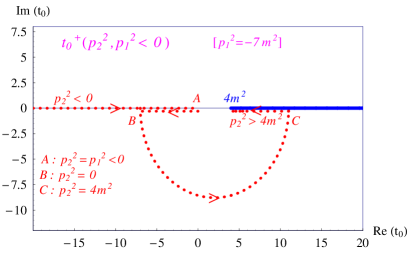
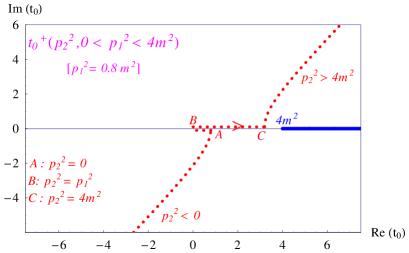
(a)                                                              (b)

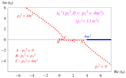
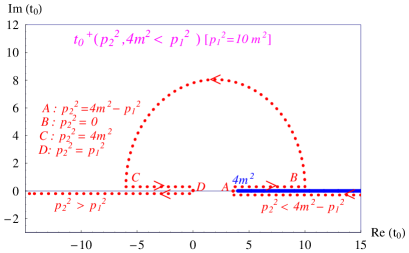
(c)                                                              (d)

Fig. 2: The trajectory of the branch point $t^{+}_{0}(p_{1}^{2},p_{2}^{2})$ vs $p_{2}^{2}$ at a fixed value of $p_{1}^{2}$ in the complex-$q^{2}$ plane. Dashed lines denote trajectories on the second (unphysical) sheet. (a) $p_{1}^{2}\leq 0$ [$p_{1}^{2}=-7m^{2}$]. (b,c) $0<p_{1}^{2}<4m^{2}$: (b) $p_{1}^{2}=0.8m^{2}$; (c) $p_{1}^{2}=3.5m^{2}$. (d) $4m^{2}<p_{1}^{2}$ [$p_{1}^{2}=10m^{2}$]. The normal cut along the real axis for $q^{2}>4m^{2}$ is depicted in blue. Noteworthy, the branch point $t^{+}_{0}(p_{1}^{2},p_{2}^{2})$ always remains on the second (unphysical) sheet of the Riemann surface and never migrates onto the physical sheet. Therefore, $t^{+}_{0}(p_{1}^{2},p_{2}^{2})$ does not influence the location of the cut on the physical sheet.

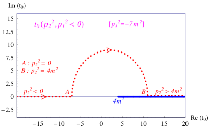
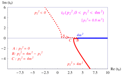
(a)                                                              (b)

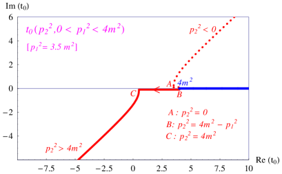
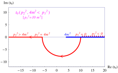
(c)                                                              (d)

Fig. 3: The trajectory of the branch point $t_{0}(p_{1}^{2},p_{2}^{2})\equiv t^{-}_{0}(p_{1}^{2},p_{2}^{2})$ vs $p_{2}^{2}$ at a fixed value of $p_{1}^{2}$ in the complex-$q^{2}$ plane: (a) $p_{1}^{2}\leq 0$ [$p_{1}^{2}=-7m^{2}$]: the (dashed line) trajectory lies on the second sheet, and does not appear on the physical sheet; (b,c) $0<p_{1}^{2}<4m^{2}$ [(b): $p_{1}^{2}=0.8m^{2}$, (c): $p_{1}^{2}=3.5m^{2}$]: the trajectory first lies on the second sheet (dashed line), but for $p_{2}^{2}>4m^{2}-p_{1}^{2}$ moves around the normal-cut branch point through the normal cut onto the physical sheet (solid line); (d) $4m^{2}<p_{1}^{2}$ [$p_{1}^{2}=10m^{2}$]: for $p_{2}^{2}<0$, the trajectory runs on the unphysical sheet, but at $p_{2}^{2}=0$ it comes up to the physical sheet and for $p_{2}^{2}>0$ travels over this physical sheet. As soon as the branch point $t_{0}(p_{1}^{2},p_{2}^{2})$ appears on the physical sheet, the $q^{2}$-integration contour should be modified such that it embraces both the normal cut and the branch point $t_{0}(p_{1}^{2},p_{2}^{2})$. The normal cut along the real axis for $q^{2}>4m^{2}$ is depicted in blue.

II.3 The branch point $t_{0}^{-}(p_{1}^{2},p_{2}^{2})$

Treated as the function of $p_{2}^{2}$ for a fixed value of $p_{1}^{2}$, the branch point $t_{0}\equiv t_{0}^{-}(p_{1}^{2},p_{2}^{2})$ has its trajectory at $p_{2}^{2}<0$ on the unphysical sheet of the complex $q^{2}$-plane. However, at some value of $p_{2}^{2}$, it crosses the cut at $t\geq 4m^{2}$. Crossing the cut means that the branch point $t_{0}$ moves onto the physical sheet through this cut. The integration contour in the Cauchi theorem is chosen on the physical sheet of complex variable $q^{2}$ and embraces (any) region of complex variable $q^{2}$, where the function $F(q^{2},p_{1}^{2},p_{2}^{2})$ of the complex variable $q^{2}$ has no singularities. The migration of the branch point $t_{0}$ onto the physical sheet pushes the integration contour away from the normal threshold and leads to the appearance of a new segment of the $q^{2}$-integration on the physical sheet lms ; procura . This new segment is called the anomalous cut. The trajectories of $t_{0}(p_{1}^{2},p_{2}^{2})$ vs $p_{2}^{2}$ for four different fixed values of $p_{1}^{2}$ are shown in Fig. 3. The dotted lines denote the segments of the trajectory lying on the unphysical sheet; the solid lines denote those segments that are on the physical sheet.

Therefore, for external momenta satisfying the relation $p_{1}^{2}>0$, $p_{2}^{2}>0$, $p_{1}^{2}+p_{2}^{2}>4m^{2}$, the integration contour in the dispersion representation for the form factor depends on the values of $p_{1}^{2}$ and $p_{2}^{2}$: the contour should be chosen such that it embraces both branch points: the normal branch point at $q^{2}=4m^{2}$ and the anomalous branch point at $q^{2}=t_{0}(p_{1}^{2},p_{2}^{2})$.

Let us consider the single dispersion representation for the form factor in the region $0<p_{1}^{2}<4m^{2}$, $0<p_{2}^{2}<4m^{2}$, and $4m^{2}<p_{1}^{2}+p_{2}^{2}$. This case corresponds to an interesting example of a two-particle bound state, and is necessary for considering the nonrelativistic expansion. The corresponding $t_{0}$-trajectory is shown in Fig. 3. Fig. 4 gives the integration contour for this case: this contour may be chosen along the real axis from $t_{0}(p_{2}^{2})$ to $+\infty$. It contains two pieces: the normal part from $4m^{2}$ to $+\infty$ and the anomalous part from $t_{0}$ to $4m^{2}$.

Let us start with the normal part, which has the form

Notice that the normal spectral density does not vanish at the normal threshold $t=4m^{2}$.

The discontinuity of the form factor $F(q^{2},p_{1}^{2},p_{2}^{2})$ on the anomalous cut is related to the discontinuity of the function $\sigma_{\rm norm}(t,p_{1}^{2},p_{2}^{2})$ and reads

$$\sigma_{\rm anom}(t,p_{1}^{2},p_{2}^{2})=\frac{1}{8\sqrt{-\lambda(t,p_{1}^{2},p_{2}^{2})}},\qquad t_{0}\leq t\leq 4m^{2}.$$ (19)

Therefore, the full spectral density has the form

$$\sigma(t,p_{1}^{2},p_{2}^{2})=\theta(p_{1}^{2}+p_{2}^{2}-4m^{2})\theta(t_{0}\leq t\leq 4m^{2})\sigma_{\rm anom}(t,p_{1}^{2},p_{2}^{2})+\theta(4m^{2}\leq t)\sigma_{\rm norm}(t,p_{1}^{2},p_{2}^{2}).$$ (20)

Clearly, the spectral density given by Eqs. (LABEL:norm) and (19) is a continuous function for $t>t_{0}$. The spectral representation for the form factor then contains the normal and the anomalous contributions:

$$F(q^{2},p_{1}^{2},p_{2}^{2})=\theta(p_{1}^{2}+p_{2}^{2}-4m^{2})\int\limits_{t_{0}(p_{1}^{2},p_{2}^{2})}^{4m^{2}}\frac{dt}{\pi(t-q^{2}-i0)}\sigma_{\rm anom}(t,p_{1}^{2},p_{2}^{2})+\int\limits_{4m^{2}}^{\infty}\frac{dt}{\pi(t-q^{2}-i0)}\sigma_{\rm norm}(t,p_{1}^{2},p_{2}^{2}).$$ (21)

For $t_{0}(p_{1}^{2},p_{2}^{2})<q^{2}<4m^{2}$ (in case $p_{1}^{2}+p_{2}^{2}>4m^{2}$) the imaginary part of the form factor comes from the anomalous part, while for $q^{2}>4m^{2}$ it comes from the normal part.

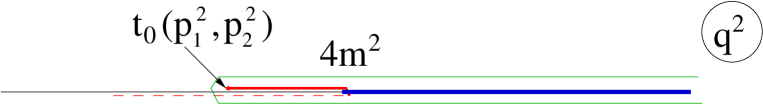
Fig. 4: The integration contour (green) in the complex $q^{2}$-plane for $0<p_{1}^{2}<4m^{2}$, $0<p_{2}^{2}<4m^{2}$, and $p_{1}^{2}+p_{2}^{2}>4m^{2}$: it embraces the anomalous cut (red), which lies along the real axis from $t_{0}$ to $4m^{2}$, and the normal cut (blue) from $4m^{2}$ to $+\infty$.

II.4 An illustration for the case of equal external masses $p_{1}^{2}=p_{2}^{2}$

Let us now specify the general formulas given above for the case of the equal “external” masses. We set $p_{1}^{2}=p_{2}^{2}=M^{2}$, and aim at obtaining the dispersion representation for the case $2m^{2}<M^{2}<4m^{2}$. Notice that both $p_{1}^{2}$ and $p_{2}^{2}$ are below the normal thresholds; the latter are located at $p_{1}^{2}=4m^{2}$ and $p_{2}^{2}=4m^{2}$. Nevertheless, we shall see that the anomalous threshold in the single dispersion representation in $q^{2}$ will emerge.

We start with calculating the spectral density in the region $M^{2}<0$, where it is given by Cutkosky rules:

$$\sigma_{\rm norm}(t,M^{2})=\frac{1}{16\pi\sqrt{t(t-4M^{2})}}\log\left(\frac{t-2M^{2}+\sqrt{t(t-4M^{2})}\sqrt{1-4m^{2}/t}}{t-2M^{2}-\sqrt{t(t-4M^{2})}\sqrt{1-4m^{2}/t}}\right),\qquad M^{2}<0.$$ (22)

It turns out that this expression is also valid in a broader domain, namely, $M^{2}<m^{2}$ (see Fig. 5a). Performing the analytic continuation in variable $M^{2}$ from the domain $M^{2}<m^{2}$, we obtain the spectral density for the region of interest $2m^{2}<M^{2}<4m^{2}$:

$$\sigma_{\rm norm}(t,M^{2})=\left\{\begin{array}[]{ll}\frac{1}{16\pi\sqrt{t(t-4M^{2})}}\log\left(\frac{t-2M^{2}+\sqrt{t(t-4M^{2})}\sqrt{1-4m^{2}/t}}{t-2M^{2}-\sqrt{t(t-4M^{2})}\sqrt{1-4m^{2}/t}}\right),&\quad 4M^{2}\leq t,\\ \frac{1}{8\pi\sqrt{-t(t-4M^{2})}}\arctan\left(\frac{\sqrt{t(t-4M^{2})}\sqrt{1-4m^{2}/t}}{t-2M^{2}}\right),&\quad 2M^{2}\leq t\leq 4M^{2},\\ \frac{1}{8\pi\sqrt{-t(t-4M^{2})}}\left[\pi+\arctan\left(\frac{\sqrt{t(t-4M^{2})}\sqrt{1-4m^{2}/t}}{t-2M^{2}}\right)\right],&\quad 4m^{2}\leq t\leq 2M^{2}.\end{array}\right.$$ (26)

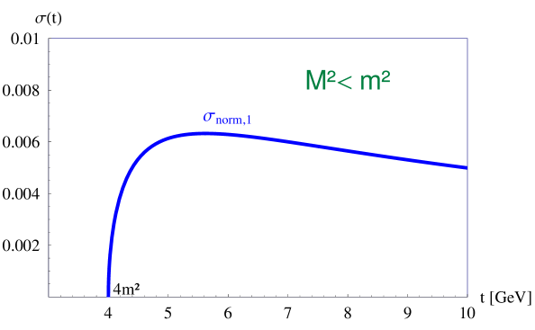
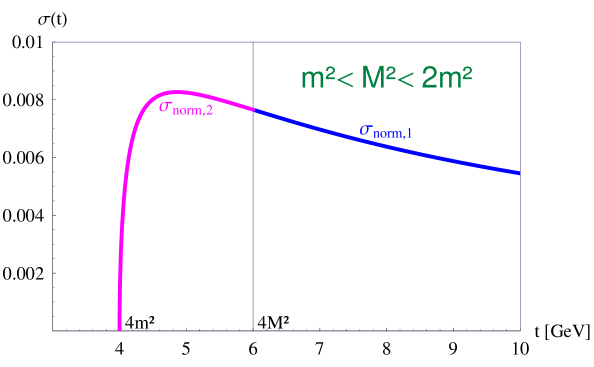
Fig. 5: The spectral density $\sigma(s,M^{2})$ for different values of $m$ and $M$. $\sigma_{\rm norm,1}$ denotes the expression in the first line of Eq. (26); $\sigma_{\rm norm,3}$ denotes the expression in the second line of Eq. (26); and $\sigma_{\rm norm,3}$ denotes the expression in the second line of Eq. (26). $\sigma_{\rm anom}$ is given by Eq. (27). Notice that for $M^{2}<2m^{2}$, two upper plots, the spectral density vanishes at the normal threshold $t=4m^{2}$, whereas in the case $M^{2}>2m^{2}$, the spectral density does not vanish neither at the normal threshold $4m^{2}$, nor at the anomalous threshold $t_{0}$.

Figure 5 (b,c) shows the cases $m^{2}<M^{2}<2m^{2}$ and $2m^{2}<M^{2}<4m^{2}$, respectively. In the latter case, the normal spectral density does not vanish at the normal threshold $t=4m^{2}$. The discontinuity of the form factor $F(q^{2},M^{2})$ on the anomalous cut is related to the discontinuity of the function $\sigma_{\rm norm}(t,M^{2})$ and reads

$$\sigma_{\rm anom}(t,M^{2})=\frac{1}{8\sqrt{-t(t-4M^{2})}},\qquad t_{0}\leq t\leq 4m^{2},\qquad t_{0}=\frac{M^{2}}{m^{2}}(4m^{2}-M^{2}).$$ (27)

Therefore, the full spectral density has the form

$$\sigma(t,M^{2})=\theta(M^{2}-2m^{2})\theta(t_{0}\leq t\leq 4m^{2})\sigma_{\rm anom}(t,M^{2})+\theta(4m^{2}\leq t)\sigma_{\rm norm}(t,M^{2}).$$ (28)

Clearly, the spectral density given by Eqs. (26) and (27) is a continuous function for $t>t_{0}$ (see Fig. 5 c).

The spectral representation for the form factor reads

$$F(q^{2},M^{2})=\theta(M^{2}-2m^{2})\int\limits_{t_{0}}^{4m^{2}}\frac{dt}{\pi(t-q^{2}-i0)}\sigma_{\rm anom}(t,M^{2})+\int\limits_{4m^{2}}^{\infty}\frac{dt}{\pi(t-q^{2}-i0)}\sigma_{\rm norm}(t,M^{2}).$$ (29)

It can be also written in the usual form

$$F(q^{2},M^{2})=\int\limits_{t_{0}}^{\infty}\frac{dt}{\pi(t-q^{2}-i0)}\sigma(t,M^{2}),$$ (30)

where $\sigma(t,M^{2})$ contains the normal and the anomalous pieces.

Figure 6 shows the calculated real parts of the normal and the anomalous contributions to the form factor $F(q^{2}=M_{R}^{2},M^{2})$ depending on the value of the mass of the decaying resonance $M_{R}^{2}=q^{2}>0$.

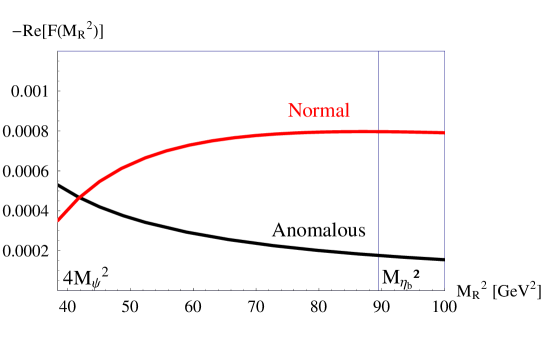
Fig. 6: The real part of the normal (red) and of the anomalous (black) contributions to the amplitude $F(q^{2}=M_{R}^{2},M^{2})$ vs $M_{R}^{2}$. Here we use the following numbers $m=m_{D}=1.87$ GeV, $M=M_{J/\psi}=3.1$ GeV, and $M_{\eta_{b}}=9.46$ GeV.

III Double dispersion representation in $p_{1}^{2}$ and $p_{2}^{2}$ for particles of mass $m$ in the loop

The previous Section presented the single dispersion representation in $q^{2}$ for the triangle diagram with particles of mass $m$ in the loop. For the same triangle diagram, a double dispersion representation in $p_{1}^{2}$ and $p_{2}^{2}$ may be written anisovich ; anisovich_melikhov ; lucha_melikhov .

At $q^{2}<0$, such a double dispersion representation in $p_{1}^{2}$ and $p_{2}^{2}$ has the form:

$$F(q^{2},p_{1}^{2},p_{2}^{2})=\int\frac{ds_{1}}{\pi(s_{1}-p_{1}^{2}-i0)}\frac{ds_{2}}{\pi(s_{2}-p_{2}^{2}-i0)}\Delta(q^{2},s_{1},s_{2}).$$ (31)

The double spectral density $\Delta(q^{2},s_{1},s_{2})$ may be obtained by placing all three particles in the loop on the mass shell and taking the off-shell external momenta $p_{1}\to\tilde{p}_{1}$, $p_{2}\to\tilde{p}_{2}$, such that $\tilde{p}_{1}^{2}=s_{1}$, $\tilde{p}_{2}^{2}=s_{2}$, and $(\tilde{p}_{1}-\tilde{p}_{2})^{2}=q^{2}$ is fixed anisovich :

$$\Delta(q^{2},s_{1},s_{2}) = \frac{1}{8\pi}\int dk_{1}dk_{2}dk_{3}\delta(\tilde{p}_{1}-k_{2}-k_{3})\delta(\tilde{p}_{2}-k_{3}-k_{1})$$ (32)

$$\times\theta(k_{1}^{0})\delta(k^{2}_{1}-m^{2})\theta(k_{2}^{0})\delta(k^{2}_{2}-m^{2})\theta(k_{3}^{0})\delta(k^{3}_{2}-m^{2}),$$

$$\quad\tilde{p}_{1}^{2}=s_{1},\quad\tilde{p}_{2}^{2}=s_{2},\quad(\tilde{p}_{1}-\tilde{p}_{2})^{2}=q^{2}.$$

Explicitly, one finds

$$\Delta(q^{2},s_{1},s_{2}) = \frac{1}{16\lambda^{1/2}(s_{1},s_{2},q^{2})}\theta\left({s_{1}-4m^{2}}\right)\theta\left({s_{2}-4m^{2}}\right)$$ (33)

$$\times\theta\left[{\left(q^{2}(s_{1}+s_{2}-q^{2})\right)^{2}-\lambda(s_{1},s_{2},q^{2})\lambda(q^{2},m^{2},m^{2})}\right].$$

The solution of the $\theta$-function gives the following allowed intervals for the integration variables $s_{1}$ and $s_{2}$:

$$4m^{2}< s_{2},$$

$$s_{1}^{-}(s_{2},q^{2})< s_{1} <s_{1}^{+}(s_{2},q^{2}),$$ (34)

where

$$s_{1}^{\pm}(s_{2},q^{2}) = s_{2}+q^{2}-\frac{s_{2}q^{2}}{2m^{2}}\pm\frac{\sqrt{s_{2}(s_{2}-4m^{2})}\sqrt{q^{2}(q^{2}-4m^{2})}}{2m^{2}}.$$ (35)

The final double dispersion representation for the triangle diagram at $q^{2}<0$ takes the form

$$F(q^{2},p_{1}^{2},p_{2}^{2})=\int\limits^{\infty}_{4m^{2}}\frac{ds_{2}}{\pi(s_{2}-p_{2}^{2}-i0)}\int\limits^{s_{1}^{+}(s_{2},q^{2})}_{s_{1}^{-}(s_{2},q^{2})}\frac{ds_{1}}{\pi(s_{1}-p_{1}^{2}-i0)}\frac{1}{16\lambda^{1/2}(s_{1},s_{2},q^{2})}.$$ (36)

Notice the relation $s_{1}^{-}(s_{2},q^{2})>4m^{2}$, which holds for all $s_{2}>4m^{2}$ at $q^{2}<0$: this guarantees that the integration region in $s_{1}$ always remains above the normal threshold. Clearly, the integration region does not depend on the values of $p_{1}^{2}$ and $p_{2}^{2}$. Essential for us is that no anomalous cuts emerge in the double dispersion representation in $p_{1}^{2}$ and $p_{2}^{2}$ for $q^{2}<0$. This makes the double dispersion representation particularly convenient for treating the triangle diagram for values of $p_{1}^{2}$ and $p_{2}^{2}$ above the thresholds. One should just take care about the appearance of the absorptive parts.

IV Double spectral representation for the decay kinematics

Now we discuss the triangle diagram with particles of different masses in the loop, $m<\mu$, and consider the decay kinematics $0<q^{2}<(\mu-m)^{2}$ braun ; melikhov . We have in mind the application to processes corresponding to the overthreshold values $p_{1}^{2}>(\mu+m)^{2}$ and $p_{2}^{2}>4m^{2}$, such as, e.g., the $K\to 3\pi$ decay. As we have seen in the previous Section, the single dispersion representation in $q^{2}$ is rather complicated for $p_{1}^{2}$ and $p_{2}^{2}$ above the two-particle thresholds already for equal masses in the loop. The situation is much worse for unequal masses in the loop. On the other hand, we shall see that the double spectral representation in $p_{1}^{2}$ and $p_{2}^{2}$ is rather simple for $q^{2}<(\mu-m)^{2}$.

We start with the region $q^{2}<0$, where the double dispersion representation has the standard form both for equal and unequal masses in the loop. We then perform the analytic continuation in $q^{2}$ and observe the appearance of the anomalous contribution in the double spectral representation.

IV.1 Transition form factor at $q^{2}<0$

For $q^{2}<0$, the double dispersion representation has a form very similar to the case of equal masses melikhov :

$$F(q^{2},p_{1}^{2},p_{2}^{2})=\int\limits^{\infty}_{4m^{2}}\frac{ds_{2}}{\pi(s_{2}-p_{2}^{2})}\int\limits^{s_{1}^{+}(s_{2},q^{2})}_{s_{1}^{-}(s_{2},q^{2})}\frac{ds_{1}}{\pi(s_{1}-p_{1}^{2})}\frac{1}{16\lambda^{1/2}(s_{1},s_{2},q^{2})},$$ (37)

where

$$s_{1}^{\pm}(s_{2},q^{2}) = \frac{s_{2}(m^{2}+\mu^{2}-q^{2})+2m^{2}q^{2}}{2m^{2}}\pm\frac{\lambda^{1/2}(s_{2},m^{2},m^{2})\lambda^{1/2}(q^{2},\mu^{2},m^{2})}{2m^{2}}.$$ (38)

A new feature compared with the case of equal masses in the loop is the appearance of the region $0<q^{2}<(\mu-m)^{2}$, which was absent in the equal-mass case. This region corresponds to the decay of a particle of mass $\mu$ to a particle of mass $m$ with the emission of a particle of mass $\sqrt{q^{2}}$.

IV.2 Transition form factors at $q^{2}>0$

The form factor in the region $0<q^{2}<(\mu-m)^{2}$ may be obtained by analytic continuation of the expression (36). Let us consider the structure of the singularities of the integrand in Eq. (37) in the complex $s_{1}$-plane for a fixed real value of $s_{2}$ in the interval $s_{2}>4m^{2}$.

Fig. 7: Singularities of the function $\Delta(q^{2},s_{1},s_{2})$ in the complex $s_{1}$ plane as a function of $s_{2}$ for $q^{2}>0$. (This corresponds to the external $s_{2}$ and the internal $s_{1}$ integration). The trajectory $s_{1}^{R}(s_{2})$ at fixed $q^{2}>0$ is shown: for $s_{2}<s_{2}^{0}$ the branch point $s_{1}^{R}(s_{2})$ remains on the unphysical sheet (dashed line), but, as soon as $s_{2}>s_{2}^{0}$, it goes onto the physical sheet and moves to the left from the left boundary of the normal cut $s_{1}^{-}$. Respectively, for $s_{2}<s_{2}^{0}$ the integration contour in the complex $s_{1}$-plane may be chosen along the interval $[s_{1}^{-},s_{1}^{+}]$. For $s_{2}>s_{2}^{0}$, however, the contour should embrace the point $s_{1}^{R}$, and therefore the integration contour contains two segments: the “anomalous” segment from $s_{1}^{R}$ to $s_{1}^{-}$, and the “normal” segment from $s_{1}^{-}$ to $s_{1}^{+}$.

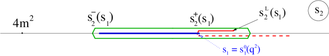
Fig. 8: Singularities of the function $\Delta(q^{2},s_{1},s_{2})$ in the complex $s_{2}$ plane as a function of $s_{1}$ for $q^{2}>0$. (This corresponds to the external $s_{1}$ and the internal $s_{2}$ integration). The trajectory $s_{2}^{L}(s_{1})$ at fixed $q^{2}>0$ is shown: for $s_{1}<s_{1}^{0}$ the branch point $s_{2}^{L}(s_{1})$ remains on the unphysical sheet (dashed line), but, as soon as $s_{1}>s_{1}^{0}$, it goes onto the physical sheet and moves to the right from the right boundary of the normal cut $s_{2}^{+}$. The notations are self-evident.

The integrand has singularities (branch points) related to the zeros of the function $\lambda(s_{1},s_{2},q^{2})$ at $s_{1}^{L}=(\sqrt{s_{2}}-\sqrt{q^{2}})^{2}$ and $s_{1}^{R}=(\sqrt{s_{2}}+\sqrt{q^{2}})^{2}$. As $q^{2}\leq 0$, these singularities lie on the unphysical sheet. However, as $q^{2}$ becomes positive, the point $s_{1}^{R}$ may move onto the physical sheet through the cut from $s_{1}^{-}$ to $s_{1}^{+}$. This happens for values of the variable $s_{2}>s_{2}^{0}$, with $s_{2}^{0}$ obtained as the solution to the equation $s_{1}^{R}(s_{2},q^{2})=s_{1}^{-}(s_{2},q^{2})$. Explicitly, one finds

$$\sqrt{s_{2}^{0}}=\frac{\mu^{2}-m^{2}-q^{2}}{\sqrt{q^{2}}}.$$ (39)

The trajectory of the point $s_{1}^{R}(s_{2},q^{2})$ in the complex $s_{1}$-plane at fixed $q^{2}>0$ vs. $s_{2}$ is shown in Fig. 7. As $q^{2}>0$, for $s_{2}>s_{2}^{0}(q^{2})$ the integration contour in the complex $s_{1}$-plane should be deformed such that it embraces the points $s_{1}^{R}$ and $s_{1}^{+}$. Respectively, the $s_{1}$-integration contour contains the two segments: the normal part from $s_{1}^{-}$ to $s_{1}^{+}$, and the anomalous part from $s_{1}^{R}$ to $s_{1}^{-}$. The double spectral density for the anomalous piece is just the discontinuity of the function $1/\sqrt{\lambda(s_{1},s_{2},q^{2})}$. It can be easily calculated as follows: Recall the relation $\sqrt{\lambda(s_{1},s_{2},q^{2})}=\sqrt{s_{1}-s_{1}^{L}}\sqrt{s_{1}-s_{1}^{R}}$. The branch point $s_{1}^{L}$ lies on the unphysical sheet, therefore the function $\sqrt{s_{1}-s_{1}^{L}}$ is continuous on the anomalous cut located on the physical sheet. Thus we have to calculate the discontinuity of the function $1/\sqrt{s_{1}-s_{1}^{R}}$ which is twice the function itself. As the result, the discontinuity of the function $1/\sqrt{\lambda(s_{1},s_{2},q^{2})}$ on the anomalous cut is $2/\sqrt{\lambda(s_{1},s_{2},q^{2})}$. Finally, the full double spectral density including the normal and the anomalous pieces takes the form

$$\Delta(q^{2},s_{1},s_{2}|\mu,m,m) = \frac{\theta(s_{2}-4m^{2})\theta(s_{1}^{-}<s_{1}<s_{1}^{+})}{16\lambda^{1/2}(s_{1},s_{2},q^{2})}+\frac{2\theta(q^{2})\theta(s_{2}-s_{2}^{0})\theta(s_{1}^{R}<s_{1}<s_{1}^{-})}{16\lambda^{1/2}(s_{1},s_{2},q^{2})}.$$ (40)

The first term in (40) relates to the Landau-type contribution emerging when all intermediate particles go on mass shell, while the second term describes the anomalous contribution.

The result (40) for $\Delta$ holds for $\mu>m$ implying the “external” $s_{2}$-integration, and the “internal” $s_{1}$-integration. The location of the integration region for this case is shown in Fig. 7. Fig. 8 gives the integration contour in the complex $s_{2}$ plane for the opposite integration order.

The final representation for the form factors at $0<q^{2}<(\mu-m)^{2}$ takes the form

$$F(q^{2},p_{1}^{2},p_{2}^{2}) = \int\limits_{4m^{2}}^{\infty}\frac{ds_{2}}{\pi(s_{2}-p_{2}^{2}-i0)}\int\limits_{s_{1}^{-}(s_{2},q^{2})}^{s_{1}^{+}(s_{2},q^{2})}\frac{ds_{1}}{\pi(s_{1}-p_{1}^{2})}\frac{1}{16\lambda^{1/2}(s_{1},s_{2},q^{2})}$$

$$+2\theta\left(0<q^{2}<(\mu-m)^{2}\right)\int\limits_{s_{2}^{0}(q^{2})}^{\infty}\frac{ds_{2}}{\pi(s_{2}-p_{2}^{2}-i0)}\int\limits_{s_{1}^{R}(s_{2},q^{2})}^{s_{1}^{-}(s_{2},q^{2})}\frac{ds_{1}}{\pi(s_{1}-p_{1}^{2})}\frac{1}{16\lambda^{1/2}(s_{1},s_{2},q^{2})}.$$

A typical behavior of the anomalous and the normal contributions is plotted in Fig. 9: the normal contribution first rises at small positive values of $q^{2}$ but then falls down steeply and vanishes at zero recoil. The anomalous contribution is zero at $q^{2}=0$, remains small at small $q^{2}>0$, but rises steeply near zero recoil, providing a smooth behavior of the full form factor.

Fig. 9: A typical behavior of the function $F(q^{2},p_{1}^{2},p_{2}^{2})$ vs. $q^{2}$ for $0<q^{2}<(\mu-m)^{2}$ at fixed $p_{1}^{2}$ and $p_{2}^{2}$. The parameters are chosen such that $(\mu-m)^{2}=1$ GeV². Dashed: normal part, solid: anomalous part, dotted: full function (sum of both parts).

We point out that the representation (IV.2) is particularly suitable for application to processes where $p_{1}^{2}$ and $p_{2}^{2}$ are above two-particle thresholds: in this case, the single spectral representation in $q^{2}$ becomes extremely complicated, with a nontrivial integration contour in the complex $q^{2}$-plane, whereas the double dispersion representation in $p_{1}^{2}$ and $p_{2}^{2}$ has the simple form given above. For values of $p_{1}^{2}$ and $p_{2}^{2}$ above the thresholds one just has to take into account the appearance of the absorptive parts in the $s_{1}$ and $s_{2}$ integrals. A possible application of this representation may be the calculation of the triangle-diagram contribution to the three-body decay anisovich_anselm_1 ; anisovich_anselm , e.g., to the $K\to 3\pi$ decay k3pi , Fig. 10. In the latter case, the diagram with the pion loop may be represented as the $\mu^{2}$ integral of the triangle diagram considered here, and one obtains the expression for the values $p_{1}^{2}=M_{K}^{2}>9m_{\pi}^{2}$, $p_{2}^{2}>4m_{\pi}^{2}$, and $q^{2}=m_{\pi}^{2}$. The emerging absorptive parts may then be easily calculated from the double spectral representation. The problem would be technically very involved if one uses the single spectral representation in $q^{2}$, as can be seen from the complicated structure of the integration contour in Section II.

Fig. 10: The triangle-diagram contribution to the $K\to 3\pi$ amplitude may be reduced to the integral over $\mu^{2}$ of the diagram $F$.

V Summary and Conclusions

I have presented a detailed analysis of dispersion representations for the triangle diagram, laying main emphasis on the appearance of the anomalous contributions in these representations. These anomalous singularities play an important role in the analysis of physical processes, see, e.g., santorelli ; oka ; mh ; as ; mm ; guo2 and a recent review guo for details. In some kinematic regions, the properties of the triangle diagram and the amplitudes of the corresponding processes are mainly determined by the anomalous contributions. A message I would like to convey to the reader is that in many cases the double spectral representations in $p_{1}^{2}$ and $p_{2}^{2}$ provide great technical advantages compared to the use of the single representation in $q^{2}$. This is clearly the case for $p_{1}^{2}$ and $p_{2}^{2}$ above the thresholds and $q^{2}$ in the decay region $0<q^{2}<(\mu-m)^{2}$. Several realistic physical cases belong to this class of problems.

Let me highlight a few points presented in this lecture:

• The single dispersion representation for the triangle diagram in the variable $q^{2}$ develops anomalous threshold, related to a migration of the logarithmic branch point from the unphysical (second) sheet of the Riemann surface onto the physical sheet through the normal $q^{2}$-cut. This migration occurs for the specific relationship between the squares of the external momenta $p_{1}^{2}$ and $p_{2}^{2}$ and the masses of the particles propagating in the loop. For instance, for the case $p_{1}^{2}=p_{2}^{2}=M^{2}$, and the particles with mass $m$ in the loop, the anomalous threshold occurs for all $M^{2}>2m^{2}$, i.e., for the external masses below the unitary thresholds $M^{2}=4m^{2}$. This means, in particular, that the anomalous thresholds occur for weakly-bound states, when $M-2m=-\epsilon_{B}$ and $\epsilon_{B}\ll m$. In this case, the location of the anomalous threshold in $q^{2}$ is responsible for the (large) radius of the weakly-bound state.

  It should be taken into account that the appearance of the anomalous cut in the single dispersion representation changes the leading singularity of the triangle diagram on the physical sheet:

  (a) In the “normal” case, $M^{2}<2m^{2}$, the spectral density of the triangle function has zero at the threshold, $\sigma(t)\sim\sqrt{t-4m^{2}}$ [Fig. 5(a,b)], thus yielding the $\sqrt{q^{2}-4m^{2}}$ leading singularity of the triangle function.

  (b) In the “anomalous” case, $2m^{2}<M^{2}$, the spectral density of the triangle function does not vanish at the anomalous threshold $t=t_{0}$ [Fig. 5(c)], thus yielding the $\log(q^{2}-t_{0})$ leading singularity. Emphasize that the logarithmic singularity does not emerge on the physical sheet in the “normal” case.

• We pointed out that at spacelike momentum transfer $q$, $q^{2}<0$, and for any values of $p_{1}^{2}$ and $p_{2}^{2}$, the double dispersion representation in $p_{1}^{2}$ and $p_{2}^{2}$ is particularly simple and contains only the normal cuts. The calculation of the triangle diagram in this case may be easily done for all values of $p_{1}^{2}$ and $p_{2}^{2}$, including the values above the thresholds and complex values. In the same situation, the single spectral representation in $q^{2}$ contains, in addition, the anomalous cut, making the application of the single dispersion representation a very involved problem.

• For the decay kinematics $0<q^{2}<(\mu-m)^{2}$, the anomalous thresholds and the anomalous cuts emerge in the double dispersion representations in the variables $p_{1}^{2}$ and $p_{2}^{2}$. In this case, the anomalous threshold in the variable $p_{1}^{2}$ (or $p_{2}^{2}$) is absent at $q^{2}<0$ but emerges for positive values of $q^{2}$. This anomalous threshold in this case lies above the normal unitary threshold at $p_{1}^{2}=(\mu+m)^{2}$ and $p_{2}^{2}=4m^{2}$. The anomalous contribution is small at small positive $q^{2}$, but steeply rises when $q^{2}$ approaches the point $q^{2}=(\mu-m)^{2}$. On the contrary, the normal contribution dominates the form factor at small $q^{2}$, but vanishes at $q^{2}=(\mu-m)^{2}$.

  In the decay region $0<q^{2}<(\mu-m)^{2}$, the double spectral representation in $p_{1}^{2}$ and $p_{2}^{2}$ provides a very convenient tool for considering processes at $p_{1}^{2}$ and $p_{2}^{2}$ above the thresholds. The application of the single spectral representation in $q^{2}$ faces in this case severe technical problems.