Frustration - Exactly Solved Frustrated Models

Abstract

After a short introduction on frustrated spin systems, we study in this chapter several two-dimensional frustrated Ising spin systems which can be exactly solved by using vertex models. We show that these systems contain most of the spectacular effects due to the frustration: high ground-state degeneracy, existence of several phases in the ground-state phase diagram, multiple phase transitions with increasing temperature, reentrance, disorder lines, partial disorder at equilibrium. Evidences of such effects in non solvable models are also shown and discussed.

I Frustration: an introduction

The study of order-disorder phenomena is a fundamental task of equilibrium statistical mechanics. Great efforts have been made to understand the basic mechanisms responsible for spontaneous ordering as well as the nature of the phase transition in many kinds of systems. In particular, during the last 25 years, much attention has been paid to frustrated models.Lieb The word ”frustration” has been introduced Tou ; Villain1 to describe the situation where a spin (or a number of spins) in the system cannot find an orientation to fully satisfy all the interactions with its neighboring spins (see below). This definition can be applied to Ising spins, Potts models and vector spins. In general, the frustration is caused either by competing interactions (such as the Villain modelVillain1 ) or by lattice structure as in the triangular, face-centered cubic (fcc) and hexagonal-close-packed (hcp) lattices, with antiferromagnetic nearest-neighbor (nn) interaction. The effects of frustration are rich and often unexpected. Many of them are not understood yet at present (see the other chapters of this book).

In addition to the fact that real magnetic materials are often frustrated due to several kinds of interactions (see the chapter by Gaulin and Gardner, this book), frustrated spin systems have their own interest in statistical mechanics. Recent studies show that many established statistical methods and theories have encountered many difficulties in dealing with frustrated systems. In some sense, frustrated systems are excellent candidates to test approximations and improve theories. Since the mechanisms of many phenomena are not understood in real systems (disordered systems, systems with long-range interaction, three-dimensional systems, etc), it is worth to search for the origins of those phenomena in exactly solved systems. These exact results will help to understand qualitatively the behavior of real systems which are in general much more complicated.

I.1 Definition

Let us give here some basic definitions to help readers unfamiliar with these subjects to read the remaining chapters of this book.

Consider two spins $\mathbf{S}_{i}$ and $\mathbf{S}_{j}$ with an interaction $J$. The interaction energy is $E=-J\left(\mathbf{S}_{i}\cdot\mathbf{S}_{j}\right)$. If $J$ is positive (ferromagnetic interaction) then the minimum of $E$ is $-J$ corresponding to the configuration in which $\mathbf{S}_{i}$ is parallel to $\mathbf{S}_{j}$. If $J$ is negative (antiferromagnetic interaction), the minimum of $E$ corresponds to the configuration where $\mathbf{S}_{i}$ is antiparallel to $\mathbf{S}_{j}$. It is easy to see that in a spin system with nn ferromagnetic interaction, the ground state (GS) of the system corresponds to the spin configuration where all spins are parallel: the interaction of every pair of spins is fully satisfied. This is true for any lattice structure. If $J$ is antiferromagnetic, the spin configuration of the GS depends on the lattice structure: i) for lattices containing no elementary triangles, i.e. bipartite lattices (such as square lattice, simple cubic lattices, …) the GS is the configuration in which each spin is antiparallel to its neighbors, i.e. every bond is fully satisfied. ii) for lattices containing elementary triangles such as the triangular lattice, the fcc lattice and the hcp lattice, one cannot construct a GS where all bonds are fully satisfied (see Fig. 1). The GS does not correspond to the minimum of the interaction of every spin pair. In this case, one says that the system is frustrated.

We consider another situation where the spin system can be frustrated: this is the case with different kinds of conflicting interactions and the GS does not correspond to the minimum of each kind of interaction. For example, consider a chain of spins where the nn interaction $J_{1}$ is ferromagnetic while the next nn (nnn) interaction $J_{2}$ is antiferromagnetic. As long as $|J_{2}|\ll J_{1}$, the GS is ferromagnetic: every nn bond is then satisfied but the nnn ones are not. Of course, when $|J_{2}|$ exceeds a critical value, the ferromagnetic GS is no longer valid (see an example below): both the nn and nnn bonds are not fully satisfied.

In a general manner, we can say that a spin system is frustrated when one cannot find a configuration of spins to fully satisfy the interaction (bond) between every pair of spins. In other words, the minimum of the total energy does not correspond to the minimum of each bond. This situation arises when there is a competition between different kinds of interactions acting on a spin by its neighbors or when the lattice geometry does not allow to satisfy all the bonds simultaneously. With this definition, the chain with nn ferromagnetic and nnn antiferromagnetic interactions discussed above is frustrated even in the case where the ferromagnetic spin configuration is its GS ($|J_{2}|\ll J_{1}$).

The first frustrated system which was studied in 1950 is the triangular lattice with Ising spins interacting with each other via a nn antiferromagnetic interactionWan . For vector spins, non collinear spin configurations due to competing interactions were first discovered in 1959 independently by YoshimoriYos , VillainVill and KaplanKapl .

Consider an elementary cell of the lattice. This cell is a polygon formed by faces hereafter called ”plaquettes”. For example, the elementary cell of the simple cubic lattice is a cube with six square plaquettes, the elementary cell of the fcc lattice is a tetrahedron formed by four triangular plaquettes. Let $J_{i,j}$ be the interaction between two nn spins of the plaquette. According to the definition of Toulouse,Tou the plaquette is frustrated if the parameter $P$ defined below is negative

$$P=\prod_{\left<i,j\right>}\mathrm{sign}(J_{i,j}),$$ (1)

where the product is performed over all $J_{i,j}$ around the plaquette. Two examples of frustrated plaquettes are shown in Fig. 1: a triangle with three antiferromagnetic bonds and a square with three ferromagnetic bonds and one antiferromagnetic bond. $P$ is negative in both cases. One sees that if one tries to put Ising spins on those plaquettes, at least one of the bonds around the plaquette will not be satisfied. For vector spins, we show below that in the lowest energy state, each bond is only partially satisfied.

Figure 1: Examples of frustrated plaquettes: ferro- and antiferromagnetic interactions, $J$ and $-J$, are shown by single and double lines, $\uparrow$ and $\downarrow$ Ising spins by black and void circles, respectively. Choosing any orientation for the spin marked by the question mark will leave one of its bonds unsatisfied (frustrated bond).

One sees that for the triangular plaquette, the degeneracy is three, and for the square plaquette it is four, in addition to the degeneracy associated with returning all spins. Therefore, the degeneracy of an infinite lattice composed of such plaquettes is infinite, in contrast to the unfrustrated case.

At this stage, we note that although in the above discussion we have taken the interaction between two spins to be of the form $E=-J\left(\mathbf{S}_{i}\cdot\mathbf{S}_{j}\right)$, the concept of frustration can be applied to other types of interactions such as the Dzyaloshinski-Moriya interaction $E=-J\left|\left(\mathbf{S}_{i}\wedge\mathbf{S}_{j}\right)\right|$: a spin system is frustrated whenever the minimum of the system energy does not correspond to the minimum of all local interactions, whatever the form of interaction. We note however that this definition of frustration is more general than the one using Eq. (1).

The determination of the GS of various frustrated Ising spin systems as well as discussions on their properties will be shown . In the following section, we analyze the GS of XY and Heisenberg spins.

I.2 Non collinear spin configurations

Let us return to the plaquettes shown in Fig. 1. In the case of $XY$ spins, one can calculate the GS configuration by minimizing the energy of the plaquette $E$ while keeping the spin modulus constant. In the case of the triangular plaquette, suppose that spin $\mathbf{S}_{i}$ $(i=1,2,3)$ of amplitude $S$ makes an angle $\theta_{i}$ with the $\mathbf{Ox}$ axis. Writing $E$ and minimizing it with respect to the angles $\theta_{i}$, one has

$$E = J(\mathbf{S}_{1}\cdot\mathbf{S}_{2}+\mathbf{S}_{2}\cdot\mathbf{S}_{3}+\mathbf{S}_{3}\cdot\mathbf{S}_{1})$$

$$= JS^{2}\left[\cos(\theta_{1}-\theta_{2})+\cos(\theta_{2}-\theta_{3})+\cos(\theta_{3}-\theta_{1})\right],$$

$$\frac{\partial E}{\partial\theta_{1}} = -JS^{2}\left[\sin(\theta_{1}-\theta_{2})-\sin(\theta_{3}-\theta_{1})\right]=0,$$

$$\frac{\partial E}{\partial\theta_{2}} = -JS^{2}\left[\sin(\theta_{2}-\theta_{3})-\sin(\theta_{1}-\theta_{2})\right]=0,$$

$$\frac{\partial E}{\partial\theta_{3}} = -JS^{2}\left[\sin(\theta_{3}-\theta_{1})-\sin(\theta_{2}-\theta_{3})\right]=0.$$

A solution of the last three equations is $\theta_{1}-\theta_{2}=\theta_{2}-\theta_{3}=\theta_{3}-\theta_{1}=2\pi/3$. One can also write

$$E=J(\mathbf{S}_{1}\cdot\mathbf{S}_{2}+\mathbf{S}_{2}\cdot\mathbf{S}_{3}+\mathbf{S}_{3}\cdot\mathbf{S}_{1})=-\frac{3}{2}JS^{2}+\frac{J}{2}(\mathbf{S}_{1}+\mathbf{S}_{2}+\mathbf{S}_{3})^{2}.$$

The minimum here evidently corresponds to $\mathbf{S}_{1}+\mathbf{S}_{2}+\mathbf{S}_{3}=0$ which yields the $120^{\circ}$ structure. This is true also for Heisenberg spins.

We can do the same calculation for the case of the frustrated square plaquette. Suppose that the antiferromagnetic bond connects the spins $\mathbf{S}_{1}$ and $\mathbf{S}_{2}$. We find

$$\theta_{2}-\theta_{1}=\theta_{3}-\theta_{2}=\theta_{4}-\theta_{3}=\frac{\pi}{4}\textrm{ and }\theta_{1}-\theta_{4}=\frac{3\pi}{4}$$ (2)

If the antiferromagnetic bond is equal to $-\eta J$, the solution for the angles isBerge

$$\cos\theta_{32}=\cos\theta_{43}=\cos\theta_{14}\equiv\theta=\frac{1}{2}[\frac{\eta+1}{\eta}]^{1/2}$$ (3)

and $|\theta_{21}|=3|\theta|$, where $\cos\theta_{ij}\equiv\cos\theta_{i}-\cos\theta_{j}$.

This solution exists if $|\cos\theta|\leq 1$, namely $\eta>\eta_{c}=1/3$. One can check that when $\eta=1$, one has $\theta=\pi/4$, $\theta_{21}=3\pi/4$.

We show the frustrated triangular and square lattices in Fig. 2 with $XY$ spins ($N=2$).

Figure 2: Non collinear spin configuration of frustrated triangular and square plaquettes with $XY$ spins: ferro- and antiferromagnetic interactions $J$ and $-J$ are indicated by thin and double lines, respectively.

One observes that there is a two-fold degeneracy resulting from the symmetry by mirror reflecting with respect to an axis, for example the $y$ axis in Fig. 2. Therefore the symmetry of these plaquettes is of Ising type O(1), in addition to the symmetry SO(2) due to the invariance by global rotation of the spins in the plane. The lattices formed by these plaquettes will be called in the following ”antiferromagnetic triangular lattice” and ”Villain lattice”, respectively.

It is expected from the GS symmetry of these systems that the transitions due to the respective breaking of O(1) and SO(2) symmetries, if they occur at different temperatures, belongs respectively to the 2D Ising universality class and to the Kosterlitz-Thouless universality class. The question of whether the two phase transitions would occur at the same temperature and the nature of their universality remains at present an open question. See more discussion in the chapter by Loison, this book.

The reader can find in Refs. [9] and [10] the derivation of the non-trivial classical ground-state configuration of the fully frustrated simple cubic lattice formed by stacking the two-dimensional Villain lattices, in the case of Heisenberg and XY spins.

Another example is the case of a chain of Heisenberg spins with ferromagnetic interaction $J_{1}(>0)$ between nn and antiferromagnetic interaction $J_{2}(<0)$ between nnn. When $\varepsilon=|J_{2}|/J_{1}$ is larger than a critical value $\varepsilon_{c}$, the spin configuration of the GS becomes non collinear. One shows that the helical configuration displayed in Fig. 3 is obtained by minimizing the interaction energy:

$$E = -J_{1}\sum_{i}\mathbf{S}_{i}\cdot\mathbf{S}_{i+1}+|J_{2}|\sum_{i}\mathbf{S}_{i}\cdot\mathbf{S}_{i+2}$$

$$= S^{2}\left[-J_{1}\cos\theta+|J_{2}|\cos(2\theta)\right]\sum_{i}1$$

$$\frac{\partial E}{\partial\theta} = S^{2}\left[J_{1}\sin\theta-2|J_{2}|\sin(2\theta)\right]\sum_{i}1=0$$ (4)

$$= S^{2}\left[J_{1}\sin\theta-4|J_{2}|\sin\theta\cos\theta\right]\sum_{i}1=0,$$

where one has supposed that the angle between nn spins is $\theta$.

The two solutions are

$$\sin\theta=0\longrightarrow\theta=0\hskip 5.69046pt\textrm{(ferromagnetic solution)}$$

and

$$\cos\theta=\frac{J_{1}}{4|J_{2}|}\longrightarrow\theta=\pm\arccos\left(\frac{J_{1}}{4|J_{2}|}\right).$$ (5)

The last solution is possible if $-1\leq\cos\theta\leq 1$, i.e. $J_{1}/\left(4|J_{2}|\right)\leq 1$ or $|J_{2}|/J_{1}\geq 1/4\equiv\varepsilon_{c}$.

Again in this example, there are two degenerate configurations: clockwise and counter-clockwise.

One defines in the following a chiral order parameter for each plaquette. For example, in the case of a triangular plaquette, the chiral parameter is given by

$$\bm{\kappa}=\frac{2}{3\sqrt{3}}\left[\mathbf{S}_{1}\wedge\mathbf{S}_{2}+\mathbf{S}_{2}\wedge\mathbf{S}_{3}+\mathbf{S}_{3}\wedge\mathbf{S}_{1}\right],$$ (6)

where coefficient $2/\left(3\sqrt{3}\right)$ was introduced so that the $\pm 2\pi/3$ degeneracy corresponds to $\kappa_{i}=\pm 1$.

Figure 3: Helical configuration when $\varepsilon=|J_{2}|/J_{1}>\varepsilon_{c}=1/4$ ($J_{1}>0$, $J_{2}<0$).

Figure 4: Antiferromagnetic triangular lattice with $XY$ spins. The positive and negative chiralities are indicated by $+$ and $-$.

We can form a triangular lattice using plaquettes as shown in Fig. 4. The GS corresponds to the state where all plaquettes of the same orientation have the same chirality: plaquettes $\bigtriangleup$ have positive chirality ($\kappa=1$) and plaquettes $\bigtriangledown$ have negative chirality ($\kappa=-1$). In terms of Ising spins, we have a perfect antiferromagnetic order. This order is broken at a phase transition temperature where $\kappa$ vanishes.

Let us enumerate two frequently encountered frustrated spin systems where the nn interaction is antiferromagnetic: the fcc lattice and the hcp lattice. These two lattices are formed by stacking tetrahedra with four triangular faces. The frustration due to the lattice structure such as in these cases is called ”geometry frustration”.

II Frustrated Ising spin systems

We are interested here in frustrated Ising spin systems without disorder. A review of early works (up to about 1985) on frustrated Ising systems with periodic interactions, i.e. no bond disorder, has been given by Liebmann.Lieb These systems have their own interest in statistical mechanics because they are periodically defined and thus subject to exact treatment. To date, very few systems are exactly solvable. They are limited to one and two dimensions (2D).Bax A few well-known systems showing remarkable properties include the centered square latticeVaks and its generalized versions,Mo ; Chi , the Kagomé lattice,Ka/Na ; Aza87 ; Diep91b an anisotropic centered honeycomb lattice,Diep91a and several periodically dilute centered square lattices.Diep92 Complicated cluster models,Kita and a particular three-dimensional case have also been solved.Horiguchi The phase diagrams in frustrated models show a rich behavior. Let us mention a few remarkable consequences of the frustration which are in connection with what will be shown in this chapter. The degeneracy of the ground state is very high, often infinite. At finite temperatures, in some systems the degeneracy is reduced by thermal fluctuations which select a number of states with largest entropy. This has been called ”Order by Disorder”,Villain/al in the Ising case. Quantum fluctuations and/or thermal fluctuations can also select particular spin configurations in the case of vector spins.Ogu ; Hen Another striking phenomenon is the coexistence of Order and Disorder at equilibrium: a number of spins in the system are disordered at all temperatures even in an ordered phase.Aza87 The frustration is also at the origin of the reentrance phenomenon. A reentrant phase can be defined as a phase with no long-range order, or no order at all, occurring in a region below an ordered phase on the temperature scale. In addition, the frustration can also give rise to disorder lines in the phase diagram of many systems as will be shown below.

In this chapter, we confine ourselves to exactly solved Ising spin systems that show remarkable features in the phase diagram such as the reentrance, successive transitions, disorder lines and partial disorder. Other Ising systems are treated in the chapter by Nagai et al. Also, the reentrance in disordered systems such as spin glasses is discussed in the chapter by Kawashima and Rieger.

The systems we consider in this chapter are periodically defined (without bond disorder). The frustration due to competing interactions will itself induce disorder in the spin orientations. The results obtained can be applied to physical systems that can be mapped into a spin language. The chapter is organized as follows. In the next section, we outline the method which allows to calculate the partition function and the critical varieties of 2D Ising models without crossing interactions. In particular, we show in detail the mapping of these models onto the 16- and 32-vertex models. We also explain a decimation method for finding disorder solutions. The purpose of this section is to give the reader enough mathematical details so that, if he wishes, he can apply these techniques to 2D Ising models with non-crossing interactions. In section 4, we shall apply the results of section 3 in some systems which present remarkable physical properties. The systems studied in section 4 contain most of interesting features of the frustration: high ground state degeneracy, reentrance, partial disorder, disorder lines, successive phase transitions, and some aspects of the random-field Ising model. In section 4 we show some evidences of reentrance and partial disorder found in three-dimensional systems and in systems with spins other than the Ising model (Potts model, classical vector spins, quantum spins). A discussion on the origin of the reentrance phenomenon and concluding remarks are given in section 5.

III Mapping between Ising models and vertex models

The 2D Ising model with non-crossing interactions is exactly soluble. The problem of finding the partition function can be transformed in a free-fermion model.If the lattice is a complicated one, the mathematical problem to solve is very cumbersome.

For numerous two-dimensional Ising models with non-crossing interactions, there exists another method, by far easier, to find the exact partition function. This method consists in mapping the model on a 16-vertex model or a 32-vertex model. If the Ising model does not have crossing interactions, the resulting vertex model will be exactly soluble. We will apply this method for finding the exact solution of several Ising models in two-dimensional lattices with non-crossing interactions.

Let us at first introduce the 16-vertex model and the 32- vertex model, and the cases for which these models satisfy the free-fermion condition.

III.1 The 16-vertex model

The 16-vertex model which we will consider is a square lattice of N points, connected by edges between neighboring sites. These edges can assume two states, symbolized by right- and left- or up-and down-pointing arrows, respectively. The allowed configurations of the system are characterized by specifying the arrangement of arrows around each lattice point. In characterizing these so-called vertex configurations, we follow the enumeration of BaxterBax ( see Fig.5).

Figure 5: Arrow configurations and vertex weights of the 16-vertex model.

To each vertex we assign an energy $\epsilon_{k}(k=1,2,...,16)$ and a corresponding vertex weight ( Boltzmann factor) $\omega_{k}=e^{\beta\epsilon_{k}}$ , where $\beta=(1)/(k_{B}T)$ , T being the temperature and $k_{B}$ the Boltzmann constant. Then the partition function is

$$Z=\sum_{C}e^{-\beta(n_{1}\epsilon_{1}+...+n_{16}\epsilon_{16})}$$ (7)

where the sum is over all allowed configurations C of arrows on the lattice, $n_{j}$ is the number of vertex arrangements of type j in configuration C. It is clear from Eq.(7) that Z is a function of the eight Boltzmann weights $\omega_{k}(k=1,2,...,16)$ :

$$Z=Z(\omega_{1},...,\omega_{16})$$ (8)

So far, exact results have only been obtained for three subclasses of the general 16-vertex model, i.e. the 6-vertex ( or ferroelectric ) model, the symmetric eight-vertex model and the free-fermion model.Bax ; Gaff Here we will consider only the case where the free-fermion condition is satisfied, because in these cases the 16-vertex model can be related to 2D Ising models without crossing interactions. Generally, a vertex model is soluble if the vertex weights satisfy certain conditions so that the partition function is reducible to the S matrix of a many-fermion system.Gaff In the present problem these constraints are the following :

$$\omega_{1} = \omega_{2}\>,\>\omega_{3}=\omega_{4}$$

$$\omega_{5} = \omega_{6}\>,\>\omega_{7}=\omega_{8}$$

$$\omega_{9} = \omega_{10}=\omega_{11}=\omega_{12}$$

$$\omega_{13} = \omega_{14}=\omega_{15}=\omega_{16}$$

$$\omega_{1}\omega_{3} + \omega_{5}\omega_{7}-\omega_{9}\omega_{11}-\omega_{13}\omega_{15}=0$$ (9)

If these conditions are satisfied, the free energy of the model can be expressed, in the thermodynamical limit, as follows :

$$f=-\frac{1}{4\pi\beta}\ \int_{0}^{2\pi}d\phi\log\{A(\phi)+[Q(\phi)]^{1/2}\}$$ (10)

where

$$A(\phi) = a+c\cos(\phi)$$

$$Q(\phi) = y^{2}+z^{2}-x^{2}-2yz\cos(\phi)+x^{2}\cos^{2}(\phi)$$

$$a = \frac{1}{2}(\omega^{2}_{1}+\omega^{2}_{3}+2\omega_{1}\omega_{3}+\omega^{2}_{5}+\omega^{2}_{7}+2\omega_{5}\omega_{7})+2(\omega^{2}_{9}+\omega^{2}_{13})$$

$$c = 2[\omega_{9}(\omega_{1}+\omega_{3})-\omega_{13}(\omega_{5}+\omega_{7})]$$

$$y = 2[\omega_{9}(\omega_{1}+\omega_{3})+\omega_{13}(\omega_{5}+\omega_{7})]$$

$$z = \frac{1}{2}[(\omega_{1}+\omega_{3})^{2}-(\omega_{5}+\omega_{7})^{2}]+2(\omega^{2}_{9}-\omega^{2}_{13})$$

$$x^{2} = z^{2}-\frac{1}{4}[(\omega_{1}-\omega_{3})^{2}-(\omega_{5}-\omega_{7})^{2}]^{2}$$ (11)

Phase transitions occur when one or more pairs of zeros of the expression $Q(\phi)$ close in on the real $\phi$ axis and ”pinch” the path of integration in the expression on the right-hand side of Eq. (10). This happens when $y^{2}=z^{2}$, i.e. when

$$\omega_{1}+\omega_{3}+\omega_{5}+\omega_{7}+2\omega_{9}+2\omega_{13}=2\mbox{max}\{\omega_{1}+\omega_{3},\omega_{5}+\omega_{7},2\omega_{9},2\omega_{13}\}$$ (12)

The type of singularity in the specific heat depends on whether

$$(\omega_{1}-\omega_{3})^{2}-(\omega_{5}-\omega_{7})^{2}\neq 0\hskip 28.45274pt(\mbox{logarithmic \, singularity})$$

or

$$(\omega_{1}-\omega_{3})^{2}-(\omega_{5}-\omega_{7})^{2}=0\hskip 28.45274pt(\mbox{inverse\, square-root\, singularity})$$ (13)

III.2 The 32-vertex model

The 32-vertex model is defined by a triangular lattice of N points, connected by edges between neighboring sites. These edges can assume two states, symbolized by an arrow pointing in or pointing out of a site. In the general case, there are 64 allowed vertex configurations. If only an odd number of arrows pointing into a site are allowed, we have 32 possible vertex configurations. This is the constraint that characterizes the 32-vertex model. To each allowed vertex configuration we assign an energy $\epsilon_{k}(k=1,2,...,32)$) and a corresponding vertex weight, defined as it is shown in Fig. 6, where $\omega=e^{-\beta\epsilon_{1}}$, $\overline{\omega}=e^{-\beta\epsilon_{2}}$, $\omega_{56}=e^{-\beta\epsilon_{3}}$, $\overline{\omega}_{56}=e^{-\beta\epsilon_{4}}$ , etc.

This notation for the Boltzmann vertex weights has been introduced by Sacco and Wu,Sacco and is used also by Baxter.Bax This model is not exactly soluble in the general case, but there are several particular cases that are soluble.Sacco Here we will consider one of such cases, when the model satisfy the free-fermion condition :

$$\omega\overline{\omega} = \omega_{12}\overline{\omega}_{12}-\omega_{13}\overline{\omega}_{13}+\omega_{14}\overline{\omega}_{14}-\omega_{15}\overline{\omega}_{15}+\omega_{16}\overline{\omega}_{16}$$

$$\omega\omega_{mn} = \omega_{ij}\omega_{kl}-\omega_{ik}\omega_{jl}+\omega_{il}\omega_{jk}$$ (14)

for all permutations i, j, k, l, m, n of 1, 2, …, 6 such that $m<n$ and $i<j<k<l$. There are 15 such permutations ( corresponding to the 15 choices of m and n ), and hence a total of 16 conditions.

The rather complicated notation for the Boltzmann weights is justified by the condensed form of the free-fermion conditions Eq. (14).

When these conditions are satisfied, the free energy in the thermodynamical limit can be expressed as

$$f=-\frac{1}{8\pi^{2}\beta}\ \int_{0}^{2\pi}d\theta\int_{0}^{2\pi}d\phi\log[\omega^{2}D(\theta,\phi)]$$ (15)

where

Figure 6: Arrow configurations and vertex weights of the 32-vertex model.

$$\omega^{2}D(\theta,\phi) = \Omega_{1}^{2}+\Omega_{2}^{2}+\Omega_{3}^{2}+\Omega_{4}^{2}-2(\Omega_{1}\Omega_{3}-\Omega_{2}\Omega_{4})\cos(\theta)$$

$$-2(\Omega_{1}\Omega_{4}-\Omega_{2}\Omega_{3})\cos(\phi)+2(\Omega_{3}\Omega_{4}-\Omega_{5}\Omega_{6})\cos(\theta+\phi)$$

$$+2(\Omega_{5}\Omega_{6}-\Omega_{1}\Omega_{2})\cos(\theta-\phi)-4a\sin(\phi)\sin(\theta+\phi)$$

$$-4b\sin(\theta)\sin(\theta+\phi)-2c\sin^{2}(\theta+\phi)-2d\sin^{2}(\theta)-2e\sin^{2}(\phi)$$

with

$$\Omega_{1} = \omega+\overline{\omega}\>,\>\hskip 28.45274pt\Omega_{2}=\omega_{25}+\overline{\omega}_{25}$$

$$\Omega_{3} = \omega_{14}+\overline{\omega}_{14}\>,\>\hskip 28.45274pt\Omega_{4}=\omega_{36}+\overline{\omega}_{36}$$

$$\Omega_{5}\Omega_{6} = \omega_{15}\omega_{24}+\overline{\omega}_{15}\overline{\omega}_{24}+\omega_{14}\overline{\omega}_{25}+\omega_{25}\overline{\omega}_{14}$$

$$a = \omega_{12}\omega_{45}+\overline{\omega}_{12}\overline{\omega}_{45}-\omega\overline{\omega}_{36}-\overline{\omega}\omega_{36}$$

$$b = \omega_{23}\omega_{56}+\overline{\omega}_{23}\overline{\omega}_{56}-\omega\overline{\omega}_{14}-\overline{\omega}\omega_{14}$$

$$c = \omega\overline{\omega}+\omega_{13}\overline{\omega}_{13}-\omega_{12}\overline{\omega}_{12}-\omega_{23}\overline{\omega}_{23}$$

$$d = \omega\overline{\omega}+\omega_{26}\overline{\omega}_{26}-\omega_{16}\overline{\omega}_{16}-\omega_{12}\overline{\omega}_{12}$$

$$e = \omega\overline{\omega}+\omega_{15}\overline{\omega}_{15}-\omega_{56}\overline{\omega}_{56}-\omega_{16}\overline{\omega}_{16}$$ (17)

The critical temperature is determined from the equation

$$\Omega_{1}+\Omega_{2}+\Omega_{3}+\Omega_{4}=2\mbox{max}(\Omega_{1},\Omega_{2},\Omega_{3},\Omega_{4})$$ (18)

We will show now how different 2D Ising models without crossing interactions can be mapped onto the 16-vertex model or the 32-vertex model, with the free-fermion condition automatically satisfied in such cases.

Let us consider at first an Ising model defined on a Kagomé lattice, with two-spin interactions between nearest neighbors (nn) and between next-nearest neighbors (nnn), $J_{1}$ and $J_{2}$, respectively, as shown in Fig. 7.

Figure 7: Kagomé lattice. Interactions between nearest neighbors and between next-nearest neighbors, $J_{1}$ and $J_{2}$, are shown by single and double bonds, respectively. The lattice sites in a cell are numbered for decimation demonstration.

The Hamiltonian is written as

$$H=-J_{1}\sum_{(ij)}\sigma_{i}\sigma_{j}-J_{2}\sum_{(ij)}\sigma_{i}\sigma_{j}$$ (19)

where and the first and second sums run over the spin pairs connected by single and double bonds, respectively.

The partition function is written as

$$Z=\sum_{\sigma}\prod_{c}\exp[K_{1}(\sigma_{1}\sigma_{5}+\sigma_{2}\sigma_{5}+\sigma_{3}\sigma_{5}+\sigma_{4}\sigma_{5}+\sigma_{1}\sigma_{2}+\sigma_{3}\sigma_{4})+K_{2}(\sigma_{1}\sigma_{4}+\sigma_{3}\sigma_{2})]$$ (20)

where $K_{1,2}=J_{1,2}/k_{B}T$ and where the sum is performed over all spin configurations and the product is taken over all elementary cells of the lattice.

Since there are no crossing bond interactions, the system can be transformed into an exactly solvable free-fermion model. We decimate the central spin of each elementary cell of the lattice. In doing so, we obtain a checkerboard Ising model with multispin interactions (see Fig. 8).

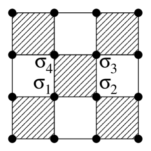
Figure 8: The checkerboard lattice. At each shaded square is associated the Boltzmann weight $W(\sigma_{1},\sigma_{2},\sigma_{3},\sigma_{4})$, given in the text.

The Boltzmann weight associated to each shaded square is given by

$$W(\sigma_{1},\sigma_{2},\sigma_{3},\sigma_{4}) = 2\cosh(K_{1}(\sigma_{1}+\sigma_{2}+\sigma_{3}+\sigma_{4}))\exp[K_{2}(\sigma_{1}\sigma_{4}+\sigma_{2}\sigma_{3})$$ (21)

$$+K_{1}(\sigma_{1}\sigma_{2}+\sigma_{3}\sigma_{4})]$$

The partition function of this checkerboard Ising model is given by

$$Z=\sum_{\sigma}\prod W(\sigma_{1},\sigma_{2},\sigma_{3},\sigma_{4})$$ (22)

where the sum is performed over all spin configurations and the product is taken over all the shaded squares of the lattice.

In order to map this model onto the 16-vertex model, let us introduce another square lattice where each site is placed at the center of each shaded square of the checkerboard lattice, as shown in Fig. 9.

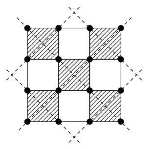
Figure 9: The checkerboard lattice and the associated square lattice with their bonds indicated by dashed lines.

At each bond of this lattice we associate an arrow pointing out of the site if the Ising spin that is traversed by this bond is equal to +1, and pointing into the site if the Ising spin is equal to -1, as it is shown in Fig. 10.

In this way, we have a 16-vertex model on the associated square lattice. The Boltzmann weights of this vertex model are expressed in terms of the Boltzmann weights of the checkerboard Ising model, as follows

$$\omega_{1} = W(-,-,+,+)\hskip 56.9055pt\omega_{5}=W(-,+,-,+)$$

$$\omega_{2} = W(+,+,-,-)\hskip 56.9055pt\omega_{6}=W(+,-,+,-)$$

$$\omega_{3} = W(-,+,+,-)\hskip 56.9055pt\omega_{7}=W(+,+,+,+)$$

$$\omega_{4} = W(+,-,-,+)\hskip 56.9055pt\omega_{8}=W(-,-,-,-)$$

$$\omega_{9} = W(-,+,+,+)\hskip 56.9055pt\omega_{13}=W(+,-,+,+)$$

$$\omega_{10} = W(+,-,-,-)\hskip 56.9055pt\omega_{14}=W(-,+,-,-)$$

$$\omega_{11} = W(+,+,-,+)\hskip 56.9055pt\omega_{15}=W(+,+,+,-)$$

$$\omega_{12} = W(-,-,+,-)\hskip 56.9055pt\omega_{16}=W(-,-,-,+)$$

Figure 10: The relation between spin configurations and arrow configurations of the associated vertex model.

Taking Eq. (21) into account, we obtain

$$\omega_{1} = \omega_{2}=2e^{-2K_{2}+2K_{1}}$$

$$\omega_{3} = \omega_{4}=2e^{2K_{2}-2K_{1}}$$

$$\omega_{5} = \omega_{6}=2e^{-2K_{2}-2K_{1}}$$

$$\omega_{7} = \omega_{8}=2e^{2K_{2}+2K_{1}}\cosh(4K_{1})$$

$$\omega_{9} = \omega_{10}=\omega_{11}=\omega_{12}=\omega_{13}=\omega_{14}=\omega_{15}=\omega_{16}=2\cosh(2K_{1})$$ (24)

As can be easily verified, the free-fermion conditions Eq. (9) are identically satisfied by the Boltzmann weights Eq. (24), for arbitrary values of $K_{1}$ and $K_{2}$. If we replace Eq. (24) in Eq. (10) and Eq. (11), we can obtain the explicit expression of the free energy of the model. Moreover, by replacing Eq. (24) in Eq. (12) we obtain the critical condition for this system :

$$\frac{1}{2}\ [\exp(2K_{1}+2K_{2})\cosh(4K_{1})+\exp(-2K_{1}-2K_{2})] +$$

$$\cosh(2K_{1}-2K_{2})+2\cosh(2K_{1})=2\mbox{max}\{\frac{1}{2}\ [\exp(2K_{1} + 2K_{2})\cosh(4K_{1})+$$

$$\exp(-2K_{1}-2K_{2})]\>;\>\cosh(2K_{2}-2K_{1}) \cosh(2K_{1})\}$$ ; (25)

which is decomposed into four critical lines depending on the values of $J_{1}$ and $J_{2}$.

The singularity of the free energy is everywhere logarithmic.

Now, we will consider another 2D Ising model with two-spin interactions and without crossing bonds. This model is defined on a centered honeycomb lattice, as shown in Fig. 11.

Figure 11: Unit cell of the centered honeycomb lattice: heavy, light, and double-light bonds denote the interactions $J_{1}$, $J_{2}$, and $J_{3}$, respectively. The sites on the honeycomb are numbered from 1 to 6 for decimation demonstration (see text).

The Hamiltonian of this model is as follows :

$$H=-J_{1}\sum_{(ij)}\sigma_{i}\sigma_{j}-J_{2}\sum_{(ij)}\sigma_{i}\sigma_{j}-J_{3}\sum_{(ij)}\sigma_{i}\sigma_{j}$$ (26)

where $\sigma_{i}=\pm 1$ is an Ising spin occupying the lattice site i , and the first, second, and third sums run over the spin pairs connected by heavy, light, and doubly light bonds, respectively ( see Fig. 11). When $J_{2}=J_{3}=0$, one recovers the honeycomb lattice, and when $J_{1}=J_{2}=J_{3}$, one has the triangular lattice.

Let us denote the central spin in a lattice cell, shown in Fig. 11, by $\sigma$, and number the other spins from $\sigma_{1}$ to $\sigma_{6}$. The Boltzmann weight associated to the elementary cell is given by

$$W=\exp[K_{1}(\sigma_{1}\sigma_{2}+\sigma_{2}\sigma_{3}+\sigma_{3}\sigma_{4}+\sigma_{4}\sigma_{5}+\sigma_{5}\sigma_{6}+\sigma_{6}\sigma_{1})+$$

$$K_{2}\sigma(\sigma_{1}+\sigma_{2}+\sigma_{4}+\sigma_{5})+K_{3}\sigma(\sigma_{3}+\sigma_{6})]$$ (27)

The partition function of the model is written as

$$Z=\sum_{\sigma}\prod_{c}W$$ (28)

where the sum is performed over all spin configurations and the product is taken over all elementary cells of the lattice. Periodic boundary conditions are imposed. Since there is no crossing-bond interaction, the model is exactly soluble. To obtain the exact solution, we decimate the central spin of each elementary cell of the lattice. In doing so, we obtain a honeycomb Ising model with multispin interactions.

After decimation of each central spin, the Boltzmann factor associated to an elementary cell is given by

$$W^{\prime}=2\exp[K_{1}(\sigma_{1}\sigma_{2}+\sigma_{2}\sigma_{3}+\sigma_{3}\sigma_{4}+\sigma_{4}\sigma_{5}+\sigma_{5}\sigma_{6}+\sigma_{6}\sigma_{1})]\times$$

$$\cosh[K_{2}(\sigma_{1}+\sigma_{2}+\sigma_{4}+\sigma_{5})+K_{3}(\sigma_{3}+\sigma_{6})]$$ (29)

We will show in the following that this model is equivalent to a special case of the 32-vertex model on the triangular lattice that satisfies the free-fermion condition.

Let us consider the dual lattice of the honeycomb lattice, i.e. the triangular lattice.Bax The sites of the dual lattice are placed at the center of each elementary cell and their bonds are perpendicular to bonds of the honeycomb lattice, as it is shown in Fig. 12.

Figure 12: The honeycomb lattice and the dual triangular lattice, with their bonds indicated by dashed lines.

Each site of the triangular lattice is surrounded by 6 sites of the honeycomb lattice. At each bond of the triangular lattice we associate an arrow. We take the arrow configuration shown in Fig. 13 as the standard one. We can establish a two-to-one correspondence between spin configurations of the honeycomb lattice and arrow configurations in the triangular lattice. This can be done in the following way : if the spins on either side of a bond of the triangular lattice are equal ( different ), place an arrow on the bond pointing in the same ( opposite ) way as the standard. If we do this for all bonds, then at each site of the triangular lattice there must be an even number of non-standard arrows on the six incident bonds, and hence an odd number of incoming ( and outgoing ) arrows. This is the property that characterize the 32 vertex model on the triangular lattice.

Figure 13: The standard arrow configuration for the triangular lattice.

In Fig. 14 we show two cases of the relation between arrow configurations on the triangular lattice and spin configurations on the honeycomb lattice.

Figure 14: Two cases of the correspondence between arrow configurations and spin configurations.

In consequence, the Boltzmann weights of the 32-vertex model will be a function of the Boltzmann weights $W^{\prime}(\sigma_{1},\sigma_{2},\sigma_{3},\sigma_{4},\sigma_{5},\sigma_{6})$ , associated to a face of the honeycomb lattice. By using the relation between vertex and spin configurations described above and expression Eq. (29), we find

$$\omega = W^{\prime}(+,-,-,-,+,+)=2e^{2K_{1}}$$

$$\overline{\omega} = W^{\prime}(+,+,-,+,+,-)=2e^{-2K_{1}}\cosh(4K_{2}-2K_{3})$$

$$\omega_{56} = W^{\prime}(+,-,+,-,+,+)=2e^{-2K_{1}}\cosh(2K_{3})$$

$$\overline{\omega}_{56} = W^{\prime}(+,+,+,+,+,-)=2e^{2K_{1}}\cosh(4K_{2})$$

$$\omega_{15} = W^{\prime}(+,+,+,-,+,+)=2e^{2K_{1}}\cosh(2K_{2}+2K_{3})$$

$$\overline{\omega}_{15} = W^{\prime}(+,-,+,+,+,-)=2e^{-2K_{1}}\cosh(2K_{2})$$

$$\omega_{46} = W^{\prime}(+,-,+,+,+,+)=2e^{2K_{1}}\cosh(2K_{2}+2K_{3})$$

$$\overline{\omega}_{46} = W^{\prime}(+,+,+,-,+,-)=2e^{-2K_{1}}\cosh(2K_{2})$$

$$\omega_{13} = W^{\prime}(+,+,+,+,-,+)=2e^{2K_{1}}\cosh(2K_{2}+2K_{3})$$

$$\overline{\omega}_{13} = W^{\prime}(+,-,+,-,-,-)=2e^{-2K_{1}}\cosh(2K_{2})$$

$$\omega_{24} = W^{\prime}(+,-,-,-,-,-)=2e^{2K_{1}}\cosh(2K_{2}+2K_{3})$$

$$\overline{\omega}_{24} = W^{\prime}(+,+,-,+,-,+)=2e^{-2K_{1}}\cosh(2K_{2})$$

$$\omega_{14} = W^{\prime}(+,+,+,+,+,+)=2e^{6K_{1}}\cosh(4K_{2}+2K_{3})$$

$$\overline{\omega}_{14} = W^{\prime}(+,-,+,-,+,-)=2e^{-6K_{1}}$$

$$\omega_{23} = W^{\prime}(+,-,-,-,+,-)=2e^{-2K_{1}}\cosh(2K_{3})$$

$$\overline{\omega}_{23} = W^{\prime}(+,+,-,+,+,+)=2e^{2K_{1}}\cosh(4K_{2})$$

$$\omega_{25} = W^{\prime}(+,-,-,+,-,-)=2e^{-2K_{1}}\cosh(2K_{3})$$

$$\overline{\omega}_{25} = W^{\prime}(+,+,-,-,-,+)=2e^{2K_{1}}$$

$$\omega_{36} = W^{\prime}(+,-,+,+,-,+)=2e^{-2K_{1}}\cosh(2K_{3})$$

$$\overline{\omega}_{36} = W^{\prime}(+,+,+,-,-,-)=2e^{2K_{1}}$$

$$\overline{\omega}_{34} = W^{\prime}(+,+,-,+,-,-)=2e^{-2K_{1}}\cosh(2K_{2}-2K_{3})$$

$$\omega_{34} = W^{\prime}(+,-,-,-,-,+)=2e^{2K_{1}}\cosh(2K_{2})$$

$$\overline{\omega}_{35} = W^{\prime}(+,+,-,-,-,-)=2e^{2K_{1}}\cosh(2K_{3})$$

$$\omega_{35} = W^{\prime}(+,-,-,+,-,+)=2e^{-2K_{1}}$$

$$\overline{\omega}_{45} = W^{\prime}(+,+,-,-,+,-)=2e^{-2K_{1}}\cosh(2K_{2}-2K_{3})$$

$$\omega_{45} = W^{\prime}(+,-,-,+,+,+)=2e^{2K_{1}}\cosh(2K_{2})$$

$$\overline{\omega}_{12} = W^{\prime}(+,-,+,-,-,+)=2e^{-2K_{1}}\cosh(-2K_{2}+2K_{3})$$

$$\omega_{12} = W^{\prime}(+,+,+,+,-,-)=2e^{2K_{1}}\cosh(2K_{2})$$

$$\overline{\omega}_{26} = W^{\prime}(+,+,+,-,-,+)=2e^{2K_{1}}\cosh(2K_{3})$$

$$\omega_{26} = W^{\prime}(+,-,+,+,-,-)=2e^{-2K_{1}}$$

$$\omega_{16} = W^{\prime}(+,+,-,-,+,+)=2e^{2K_{1}}\cosh(2K_{2})$$

$$\overline{\omega}_{16} = W^{\prime}(+,-,-,+,+,-)=2e^{-2K_{1}}\cosh(2K_{2}-2K_{3})$$ (30)

Using the above expressions in Eqs. (15), (LABEL:eq16) and (17) we can obtain the expression of the free energy of the centered honeycomb lattice Ising model.

Taking into account Eqs. (30), (17) and (18), the critical temperature of the model is determined from the equation :

$$e^{2K_{1}}+e^{-2K_{1}}\cosh(4K_{2}-2K_{3}) + 2e^{-2K_{1}}\cosh(2K_{3})+2e^{2K_{1}}+$$

$$e^{6K_{1}}\cosh(4K_{2}+2K_{3})+e^{-6K_{1}} = 2\mbox{max}\{e^{2K_{1}}+e^{-2K_{1}}\cosh(4K_{2}-2K_{3})\>\>;\>\>$$

$$e^{2K_{1}}+e^{-2K_{1}}\cosh(2K_{3}) e^{6K_{1}}\cosh(4K_{1}+2K_{3})+e^{-6K_{1}}\}$$ ; (31)

The solutions of this equation are analyzed in the next section.

We think that with the two cases studied above, the reader will be able to apply this procedure to other 2D Ising models without crossing bonds as, for instance, the Ising model on the centered square lattice. After decimation of the central spin in each square, this model can be mapped into a special case of the 16-vertex model, by following the same procedure that we have employed for the honeycomb lattice model.

III.3 Disorder solutions for two-dimensional Ising models

Disorder solutions are very useful for clarifying the phase diagrams of anisotropic models and also imply constraints on the analytical behavior of the partition function of these models.

A great variety of anisotropic models ( with different coupling constants in the different directions of the lattice ) are known to posses remarkable submanifolds in the space of parameters, where the partition function is computable and takes a very simple form. These are the disorder solutions.

All the methods applied for obtaining these solutions rely on the same mechanism : a certain local decoupling of the degrees of freedom of the model, which results in an effective reduction of dimensionality for the lattice system. Such a property is provided by a simple local condition imposed on the Boltzmann weights of the elementary cell generating the lattice.Mail

Some completely integrable models present disorder solutions, e.g. the triangular Ising model and the symmetric 8-vertex model. But very important models that are not integrable, also present this type of solutions, e.g. the triangular Ising model with a field, the triangular q-state Potts model, and the general 8-vertex model. Here we will consider only two dimensional Ising models.

In order to introduce the method, we will analyze, at the first place, the simplest case, i.e. the anisotropic Ising model on the triangular lattice ( see Fig. 15).

Figure 15: The elementary cell of the triangular lattice, with three interactions $K_{1}$, $K_{2}$, and $K_{3}$.

The Boltzmann weight of the elementary cell is

$$W(\sigma_{1},\sigma_{2},\sigma_{3})=\exp[\frac{1}{2}(K_{1}\sigma_{1}\sigma_{3}+K_{2}\sigma_{2}\sigma_{3}+K_{3}\sigma_{1}\sigma_{2})]$$ (32)

In every case, the local criterion will be defined by the following condition : after summation over some of its spins ( to be defined in each case ) , the Boltzmann weight associated with the elementary cell of the model must not depend on the remaining spins any longer. For instance, for the triangular lattice, we will require

$$\sum_{\sigma_{3}}W(\sigma_{1},\sigma_{2},\sigma_{3})=\lambda(K_{1},K_{2},K_{3})$$ (33)

where $\lambda$ is a function only of $K_{1}$, $K_{2}$ and $K_{3}$ ( it is independent of $\sigma_{1}$ and $\sigma_{2}$). By using Eq. (32) we find

$$\sum_{\sigma_{3}}W(\sigma_{1},\sigma_{2},\sigma_{3})=\exp(\frac{1}{2}K_{3}\sigma_{1}\sigma_{2})\cosh[\frac{1}{2}(K_{1}\sigma_{1}+K_{2}\sigma_{2})]$$ (34)

But, as it is well known, we can write

$$\cosh[\frac{1}{2}(K_{1}\sigma_{1}+K_{2}\sigma_{2})]=A\exp(K\sigma_{1}\sigma_{2})$$ (35)

with

$$A=[\cosh(\frac{K_{1}+K_{2}}{2})\cosh(\frac{K_{1}-K_{2}}{2})]^{\frac{1}{2}}$$ (36)

$$K=\frac{1}{2}\log[\frac{\cosh(\frac{K_{1}+K_{2}}{2})}{\cosh(\frac{K_{1}-K_{2}}{2})}]$$ (37)

In order that $\sum_{\sigma_{3}}W(\sigma_{1},\sigma_{2},\sigma_{3})$ be independent of $\sigma_{1}$ and $\sigma_{2}$ we must impose the condition $K=-\frac{1}{2}K_{3}$. From this condition we find

$$e^{K_{3}}\cosh(\frac{K_{1}+K_{2}}{2})=\cosh(\frac{K_{1}-K_{2}}{2})$$ (38)

from which we can determine the expression of $\lambda$:

$$\lambda(K_{1},K_{2},K_{3})=[\cosh(\frac{K_{1}+K_{2}}{2})\cosh(\frac{K_{1}-K_{2}}{2})]^{\frac{1}{2}}$$ (39)

It is easy to verify that Eq.(38) can be written as

$$\tanh(K_{1})\tanh(K_{2})+\tanh(K_{3})=0$$ (40)

This 2D subvariety in the space of parameters is called the disorder variety of the model.

Let us now impose particular boundary conditions for the lattice ( see Fig. 16) : on the upper layer, all interactions are missing, so that the spins of the upper layer only interact with those of the lower one. It immediately follows that if one sums over all the spins of the upper layer and if one requires the disorder condition Eq. (40) , the same boundary conditions reappear for the next layer.

Iterating the procedure leads one to an exact expression for the partition function, when restricted to subvariety Eq. (40):

$$Z=\lambda(K_{1},K_{2},K_{3})^{N}$$ (41)

Figure 16: Two layers of the triangular lattice.

where $N$ is the number of sites of the lattice. The free energy in the thermodynamic limit is given by

$$f=-\frac{1}{2\beta}\log[\cosh(\frac{K_{1}+K_{2}}{2})\cosh(\frac{K_{1}-K_{2}}{2})]$$ (42)

The partition function Eq. (41) corresponds to lattices with unusual boundary conditions. In the physical domain, where the coupling constants are real, these do not affect the partition function per site ( or the free energy per site) in the thermodynamic limit, and the expression Eq. (42) also corresponds to the free energy per site with standard periodic boundary conditions. On the contrary, in the non-physical domain ( complex coupling constants), the boundary conditions are known to play an important role, even after taking the thermodynamic limit.

Let us consider now the Kagomé lattice Ising model with two-spin interactions between nn and nnn, studied in the next section. If we apply the same procedure that for the triangular lattice Ising model, we obtain for the disorder variety:

$$e^{4K_{2}}=\frac{2(e^{4K_{1}}+1)}{e^{8K_{1}}+3}$$ (43)

This disorder variety does not have intersection with the critical variety of the model.

Following the method that we have exposed for the Ising model on the triangular lattice, the reader will be able to find the disorder varieties for other 2D Ising models with anisotropic interactions.

IV Reentrance in exactly solved frustrated Ising spin systems

In this section, we show and discuss the phase diagrams of several selected 2D frustrated Ising systems that have been recently solved. For general exact methods, the reader is referred to the book by Baxter,Bax and to the preceding section. In the following, we consider only frustrated systems that exhibit the reentrance phenomenon. A reentrant phase can be defined as a phase with no long-range order, or no order at all, occurring in a region below an ordered phase on the temperature ($T$) scale. A well-known example is the reentrant phase in spin-glasses (see the review by Binder and YoungBin ). The origin of the reentrance in spin-glasses is not well understood. It is believed that it is due to a combination of frustration and bond disorder. In order to see the role of the frustration alone, we show here the exact results on a number of periodically frustrated Ising systems. The idea behind the works shown in this section is to search for the ingredients responsible for the occurrence of the reentrant phase. Let us review in the following a few models showing a reentrant phase. Discussion on the origin of the reentrance will be given in the conclusion.

IV.1 Centered square lattice

Even before the concept of frustration was introduced,Tou systems with competing interactions were found to possess rich critical behavior and non-trivial ordered states. Among these models, the centered square lattice Ising model (see Fig. 17), introduced by Vaks et al,Vaks with nn and nnn interactions, $J_{1}$ and $J_{2}$, respectively, is to our knowledge the first exactly soluble model which exhibits successive phase transitions with a reentrant paramagnetic phase at low $T$. Exact expression for the free energy, some correlation functions, and the magnetization of one sublattice were given in the original work of Vaks et al.

Figure 17: Centered square lattice. Interactions between nn and nnn, $J_{1}$ and $J_{2}$, are denoted by white and black bonds, respectively. The two sublattices are numbered 1 and 2.

We distinguish two sublattices 1 and 2. Sublattice 1 contains the spins at the square centers, and sublattice 2 generates a square lattice with interaction $J_{2}$ in both horizontal and vertical directions. Spins of sublattice 1 interacts only with spins of sublattice 2 via diagonal interactions $J_{1}$. The ground state properties of this model are as follows : for $a=J_{2}/\mid J_{1}\mid>-1$, spins of sublattice 2 orders ferromagnetically and the spins of sublattice 1 are parallel (antiparallel) to the spins of sublattice 2 if $J_{1}>0$ ( $<0$ ); for $a<-1$, spins of sublattice 2 orders antiferromagnetically, leaving the centered spins free to flip.

IV.1.1 Phase diagram

The phase diagram of this model is given by Vaks et al.Vaks Except for $a=-1$ , there is always a finite critical temperature.

When $J_{2}$ is antiferromagnetic ($>0$) and $J_{2}/J_{1}$ is in a small region near 1, the system is successively in the paramagnetic state, an ordered state, the reentrant paramagnetic state, and another ordered state, with decreasing temperature (see Fig. 18).

Figure 18: Phase diagram of centered square lattice Vaks .

The centered square Ising lattice has been generalized to include several kinds of interaction.Mo ; Chi For example, when the vertical interaction $J_{2}$ is different from the horizontal one, say $J_{3}$, the phase diagram becomes more complicated.

IV.1.2 Nature of ordering and disorder solutions

For the sake of simplicity, let us consider hereafter the case of nn and nnn interactions only, namely $J_{1}$ and $J_{2}$ ($J_{3}=J_{2}$). Note that though an exact critical line was obtained,Vaks the order parameter was not calculated, though the magnetization of one sublattice were given in the original work of Vaks et al.Vaks Later, Choy and Baxter Choy have obtained the total magnetization for this model in the ferromagnetic region. However, the ordering in the antiferromagnetic (frustrated) region has not been exactly calculated, despite the fact that it may provide an interesting ground for understanding the reentrance phenomenon. We have studied this aspect by means of Monte Carlo (MC) simulations.Aza89a The question which naturally arises is whether or not the disorder of sublattice 1 at $T=0$ remains at finite $T$. If the spins of sublattice 1 remains disordered at finite $T$ in the antiferromagnetic region we have a remarkable kind of ordered state: namely the coexistence between order and disorder. This behavior has been observed in three-dimensional Ising spin modelsBlan ; Diep85b and in an exactly soluble model (the Kagomé lattice).Aza87 In the latter system, which is similar to the present model (discussed in the next subsection), it was shown that the coexistence of order and disorder at finite $T$ shed some light on the reentrance phenomena. To verify the coexistence between order and disorder in the centered square lattice, we have performed Monte Carlo (MC) simulations. The results for the Edwards-Anderson sublattice order parameters $q_{i}$ and the staggered susceptibility of sublattice 2 , as functions of $T$, are shown in Fig. 19 in the case $a=-2$.

Figure 19: Temperature dependence of sublattice Edwards-Anderson order parameters, $q_{1}$ and $q_{2}$ (crosses and black circles, respectively) in the case $a=J_{2}/\mid J_{1}\mid=-2$, by Monte Carlo simulation. Susceptibility calculated by fluctuations of magnetization of sublattice 2 is also shown. The lattice used contains $N=2\times 60\times 60$ spins with periodic boundary conditions.

Aza89a

As is seen, sublattice 2 is ordered up to the transition at $T_{c}$ while sublattice 1 stays disordered at all $T$. This result shows a new example where order and disorder coexists in an equilibrium state. This result supports the conjecture formulated by Azaria et al, Aza87 namely the coexistence of order and disorder is a necessary condition for the reentrant behavior to occur. The partial disorder just compensates the loss of entropy due to the partial ordering of the high-$T$ phase. In a previous paper,Aza87 the importance of the disorder line in understanding the reentrance phenomenon has been emphasized. There has been suggested that this type of line may be necessary for the change of ordering from the high-$T$ ordered phase to the low-$T$ one. In the narrow reentrant paramagnetic region, preordering fluctuations with different symmetries exist near each critical line. Therefore the correlation functions change their behavior as the temperature is varied in the reentrant paramagnetic region. As a consequence of the change of symmetries there exist spins for which the two-point correlation function (between nn spins) has different signs, near the two critical lines , in the reentrant paramagnetic region. Hence it is reasonable to expect that it has to vanish at a disorder temperature $T_{D}$ . This point can be considered as a non-critical transition point which separates two different paramagnetic phases. The two-point correlation function defined above may be thought of as a non-local ’disorder parameter’. This particular point is just the one which has been called a disorder point by StephensonSte in analyzing the behavior of correlation functions for systems with competing interactions. For the centered square lattice Ising model considered here, the Stephenson disorder line isAza89a

$$\cosh(4J_{1}/k_{B}T_{D})=\exp(-4J_{2}/k_{B}T_{D})$$ (44)

The two-point correlation function at $T_{D}$ between spins of sublattice 2 separated by a distance r is zero for odd r and decay like $r^{-1/2}[\tanh(J_{2}/k_{B}T_{D})]^{r}$ for r even.Ste However,there is no dimensional reduction on the Stephenson line given above. Usually, one defines the disorder point as the temperature where there is an effective reduction of dimensionality in such a way that physical quantities become simplified spectacularly.Mail In general, these two types of disorder line are equivalent, as for example , in the case of the Kagomé lattice Ising model (see below). This is not the case here. In order to calculate this disorder line for the centered square lattice, we recall that this model is equivalent to an 8-vertex model that verifies the free-fermion condition.Wu The disorder line corresponding to dimensional reduction, was given for the general 8-vertex model by Giacomini.Giaco86 When this result is applied to the centered square lattice, one finds that the disorder variety is given by

$$\exp(4J_{2}/k_{B}T)=(1-i\sinh(4J_{1}/k_{B}T))^{-1}$$ (45)

where $i^{2}=-1$. This disorder line lies on the unphysical (complex) region of the parameter space of this system. When calculated on the line Eq. (45), the magnetization of this model, evaluated recently by Choy and Baxter Choy in the ferromagnetic region, becomes singular, as it is usually the case for the disorder solutions with dimensional reduction.Bax86 Since in the centered square lattice, the two kinds of disorder line are not equivalent, we conclude, according to the arguments presented above, that the Stephenson disorder line Eq. (44) is the relevant one for the reentrance phenomenon.

Disorder solutions have recently found interesting applications, as for example in the problem of cellular automata (for a review see RujanRujan ). Moreover, they also serve to built a new kind of series expansion for lattice spin systems.Mail

IV.2 Kagomé lattice

IV.2.1 Model with nn and nnn interactions

Another model of interest is the Kagomé lattice shown in Fig. 7. The Kagomé Ising lattice with nn interaction $J_{\rm 1}$ has been solved a long time agoKa/Na showing no phase transition at finite $T$ when $J_{1}$ is antiferromagnetic. Taking into account the nnn interaction $J_{2}$ [see Fig.7 and Eq. (19)], we have solvedAza87 this model by transforming it into a 16-vertex model which satisfies the free-fermion condition.

The critical condition is given by Eq. (25). For the whole phase diagram, the reader is referred to the paper by Azaria et al.Aza87 We show in Fig. 20 only the small region of $J_{2}/J_{1}$ in the phase diagram which has the reentrant paramagnetic phase and a disorder line.

Figure 20: Phase diagram of the Kagomé lattice with nnn interaction in the region $J_{1}>0$ of the space ($\alpha=J_{2}/J_{1},T$). $T$ is measured in the unit of $J_{1}/k_{B}$. Solid lines are critical lines, dashed line is the disorder line. P, F and X stand for paramagnetic, ferromagnetic and partially disordered phases, respectively. The inset shows schematically enlarged region of the endpoint.

The phase X indicates a partially ordered phase where the central spins are free (the nature of ordering was determined by MC simulations).Aza87 Here again, the reentrant phase takes place between a low-$T$ ordered phase and a partially disordered phase. This suggests that a partial disorder at the high-$T$ phase is necessary to ensure that the entropy is larger than that of the reentrant phase.

IV.2.2 Generalized Kagomé lattice

When all the interactions are different in the model shown in Fig. 7, i.e. the horizontal bonds $J_{3}$, the vertical bonds $J_{2}$ and the diagonal ones are not equal (see Fig. 21), the phase diagram becomes complicated with new features:Diep91b in particular, we show that the reentrance can occur in an infinite region of phase space. In addition, there may be several reentrant phases occurring for a given set of interactions when $T$ varies.

The Hamiltonian is written as

$$H=-J_{1}\sum_{(ij)}\sigma_{i}\sigma_{j}-J_{2}\sum_{(ij)}\sigma_{i}\sigma_{j}-J_{3}\sum_{(ij)}\sigma_{i}\sigma_{j}$$ (46)

where $\sigma_{i}=\pm 1$ is an Ising spin occupying the lattice site i , and the first, second, and third sums run over the spin pairs connected by diagonal, vertical and horizontal bonds, respectively. When $J_{2}=0$ and $J_{1}=J_{3}$, one recovers the original nn Kagomé lattice.Ka/Na The effect of $J_{2}$ in the case $J_{1}=J_{3}$ has been shown above.

Figure 21: Left: Generalized Kagomé lattice: diagonal, vertical and horizontal bonds denote the interactions $J_{1}$, $J_{2}$ and $J_{3}$, respectively. Right: Phase diagram of the ground state shown in the plane ($\alpha=J_{2}/J_{1},\beta=J_{3}/J_{1}$). Heavy lines separate different phases and spin configuration of each phase is indicated (up, down and free spins are denoted by +, - and o, respectively). The three kinds of partially disordered phases and the ferromagnetic phase are denoted by I, II , III and F, respectively.

The phase diagram at temperature $T=0$ is shown in Fig. 21 in the space ($\alpha=J_{2}/J_{1}$, $\beta=J_{3}/J_{1}$) for positive $J_{1}$. The ground- state spin configurations are also displayed. The hatched regions indicate the three partially disordered phases (I, II, and III) where the central spins are free. Note that the phase diagram is mirror-symmetric with respect to the change of the sign of $J_{1}$. With negative $J_{1}$ , it suffices to reverse the central spin in the spin configuration shown in Fig. 21. Furthermore, the interchange of $J_{2}$ and $J_{3}$ leaves the system invariant, since it is equivalent to a $\pi/2$ rotation of the lattice. Let us consider the effect of the temperature on the phase diagram shown in Fig. 21. Partial disorder in the ground state often gives rise to the reentrance phenomenon as in systems shown above. Therefore, similar effects are to be expected in the present system. As it will be shown below, we find a new and richer behavior of the phase diagram: in particular, the reentrance region is found to be extended to infinity, unlike systems previously studied, and for some given set of interactions, there exist two disorder lines which divide the paramagnetic phase into regions of different kinds of fluctuations with a reentrant behavior.

Following the method exposed in section 3, one obtains a checkerboard Ising model with multispin interactions. This resulting model is equivalent to a symmetric 16-vertex model which satisfies the free-fermion condition.Gaff ; Suzu ; Wu72 The critical temperature of the model is given by

$$\cosh(4K_{1})\exp(2K_{2}+2K_{3})+\exp(-2K_{2}-2K_{3})=2\cosh(2K_{3}-2K_{2})\pm 4\cosh(2K_{1})$$ (47)

Note that Eq. (47) is invariant when changing $K_{1}\rightarrow-K_{1}$ and interchanging $K_{2}$ and $K_{3}$ as stated earlier. The phase diagram in the three-dimensional space ($K_{1},K_{2},K_{3}$) is rather complicated to show. Instead, we show in the following the phase diagram in the plane ($\beta=J_{3}/J_{1},T$) for typical values of $\alpha=J_{2}/J_{1}$. To describe each case and to follow the evolution of the phase diagram, let us go in the direction of decreasing $\alpha$ :

A. $\alpha>0$

This case is shown in Fig. 22. Two critical lines are found with a paramagnetic reentrance having a usual shape (Fig. 22a) between the partially disordered (PD) phase of type III (see Fig. 21) and the ferromagnetic (F) phase with an endpoint at $\beta=-1$. The width of the reentrance region $[-1,\beta_{1}]$ decreases with decreasing $\alpha$ , from $\beta_{1}=0$ for $\alpha$ at infinity to $\beta_{1}=-1$ for $\alpha=0$ (zero width). Note that as $\alpha$ decreases, the PD phase III is depressed and disappears at $\alpha=0$, leaving only the F phase (one critical line, see Fig. 22b). The absence of order at zero $\alpha$ for $\beta$ smaller than -1 results from the fact that in the ground state, this region of parameters corresponds to a superdegenerate line separating the two PD phases II and III (see Fig. 21). So, along this line, the disorder contaminates the system for all $T$. As for disorder solutions, for positive $\alpha$ we find in the reentrant paramagnetic region a disorder line with dimension reductionSte given by

$$\exp(4K_{3})=2\cosh(2K_{2})/[\cosh(4K_{1})\exp(2K_{2})+\exp(-2K_{2})]$$ (48)

This is shown by the dotted lines in Fig. 22.

Figure 22: Phase diagram in the plane ($\beta=J_{3}/J_{1},T$) for positive values of $\alpha=J_{2}/J_{1}$:(a) $\alpha=1$, (b) $\alpha=0$. Solid lines are critical lines which separate different phases: paramagnetic (P), ferromagnetic (F), partially disordered phase of type III (III). Dotted line shows the disorder line.

B. $0>\alpha>-1$

In this range of $\alpha$, there are three critical lines. The critical line separating the F and P phases and the one separating the PD phase I from the P phase have a common horizontal asymptote as $\beta$ tends to infinity . They form a reentrant paramagnetic phase between the F phase and the PD phase I for positive b between a value $\beta_{2}$ and infinite $\beta$ (Fig. 23). Infinite region of reentrance like this has never been found before this model. As $\alpha$ decreases, $\beta_{2}$ tends to zero and the F phase is contracted. For $\alpha<-1$, the F phase disappears together with the reentrance.

Figure 23: Phase diagram in the plane ($\beta=J_{3}/J_{1},T$) for negative values of $\alpha=J_{2}/J_{1}$. Left: $\alpha=-0.25$, Right: $\alpha=-0.8$. Solid lines are critical lines which separate different phases: paramagnetic (P), ferromagnetic (F), partially disordered phases of type I and III. Dotted lines show the disorder lines.

In the interval $0>\alpha>-1$, the phase diagram possesses two disorder lines, the first being given by Eq. (48), and the second by

$$\exp(4K_{3})=2\sinh(2K_{2})/[-\cosh(4K_{1})\exp(2K_{2})+\exp(-2K_{2})]$$ (49)

These two disorder lines are issued from a point near $\beta=-1$ for small negative $\alpha$; this point tends to zero as $\alpha$ tends to -1. The disorder line given by Eq. (49) enters the reentrant region which separates the F phase and the PD phase I (Fig. 23, left), and the one given by Eq. (48) tends to infinity with the asymptote $\beta=0$ as $T\rightarrow\infty$. The most striking feature is the behavior of these two disorder lines at low $T$: they cross each other in the P phase for $0>\alpha>-0.5$, forming regions of fluctuations of different nature (Fig. 24a). For $-0.5>\alpha>-1$, the two disorder lines do no longer cross each other (see Fig. 24b). The one given by Eq. (48) has a reentrant aspect: in a small region of negative values of $\beta$, one crosses three times this line in the P phase with decreasing $T$.

Figure 24: The behavior of the disorder lines (dotted) is schematically enlarged in the case (a) $\alpha=-0.25$, (b) $\alpha=-0.8$, (c) $\alpha=-1.5$.

C. $\alpha\leq-1$

For $\alpha$ smaller than -1, there are two critical lines and no reentrance (Fig. 25). Only the disorder line given by Eq. (48) survives with a reentrant aspect: in a small region of negative values of $\beta$, one crosses twice this line in the P phase with decreasing $T$. This behavior, being undistiguishable in the scale of Fig. 25, is schematically enlarged in Fig. 24c. The multicritical point where the P, I and II phases meet is found at $\beta=0$ and $T=0$.

Figure 25: The same caption as that of Fig. 23 with (a) $\alpha=-1$, (b) $\alpha=-1.5$.

At this stage, it is interesting to note that while reentrance and disorder lines occur along the horizontal axis $\alpha=-1$ and along the vertical axis $\beta=-1$ of Fig. 21 when the temperature is switched on, the most frustrated region ($\alpha<0$ and $\beta<0$) of the ground state does not show successive phase transitions (see Fig. 25, for example). Therefore, the existence of a reentrance may require a sufficient frustration, but not overfrustration. Otherwise, the system may have either a PD phase (Fig. 25) or no order at all (Fig. 22b).

The origin of the reentrance phenomenon will be discussed again in the conclusion.

IV.3 Centered honeycomb lattice

In order to find common aspects of the reentrance phenomenon, we have constructed a few other models which possess a partially disordered phase next to an ordered phase in the ground state. Let us mention here the anisotropic centered honeycomb lattice shown in Fig. 11.Diep91a The Hamiltonian is given by Eq. (25), with three kinds of interactions $J_{1}$, $J_{2}$, and $J_{3}$ denoting the interactions between the spin pairs connected by heavy, light, and double-light bonds, respectively. We recall that when $J_{2}=J_{3}=0$, one recovers the honeycomb lattice, and when $J_{1}=J_{2}=J_{3}$ one has the triangular lattice.

Fig. 26 shows the phase diagram at temperature $T=0$ for three cases ($J_{1}\neq J_{2}=J_{3}$), ( $J_{1}\neq J_{3},J_{2}=0$) and ($J_{1}\neq J_{2},J_{3}=0$). The ground-state spin configurations are also indicated.

The phase diagram is symmetric with respect to the horizontal axis: the transformation $(J_{2},\sigma)\rightarrow(-J_{2},-\sigma)$ , or $(J_{3},\sigma)\rightarrow(-J_{3},-\sigma)$ , leaves the system invariant. In each case, there is a phase where the central spins are free to flip (”partially disordered phase”). In view of this common feature with other models studied so far, one expects a reentrant phase occurring between the partially disordered phase and its neighboring phase at finite $T$. As it will be shown below, though a partial disorder exists in the ground state, it does not in all cases studied here yield a reentrant phase at finite $T$. Only the case ($J_{1}\neq J_{2},J_{3}=0$) does show a reentrance.

Figure 26: Phase diagram of the ground state shown in the space: (a) ($J_{1},J_{2}=J_{3}$) ; (b) ($J_{1},J_{3}$) with $J_{2}=0$) ; (c) ($J_{1},J_{2}$) with $J_{3}=0$). Heavy lines separate different phases and spin configuration of each phase is indicated (up, down and free spins are denoted by +, - and o, respectively).

To obtain the exact solution of our model, we decimate the central spin of each elementary cell of the lattice as outlined in the section 3. The resulting model is equivalent to a special case of the 32-vertex modelSacco on a triangular lattice that satisfies the free-fermion condition. The explicit expression of the free energy as a function of interaction parameters $K_{1}$, $K_{2}$, and $K_{3}$ is very complicated, as seen by replacing Eq. (29) in Eqs. (15), (LABEL:eq16) and (17). The critical temperature is given by Eq. (30).

We have analyzed, in particular, the three cases ($K_{1}\neq K_{2}=K_{3}$) , ($K_{1}\neq K_{3},K_{2}=0$) and ($K_{1}\neq K_{2},K_{3}=0$).

When $K_{2}=K_{3}$, the critical line obtained from Eq.(30) is

$$\exp(3K_{1})\cosh(6K_{2})+\exp(-3K_{1})=3[\exp(K_{1})+\exp(-K_{1})\cosh(2K_{2})]$$ (50)

In the case $K_{2}=0$, the critical line is given by

$$\exp(3K_{1})\cosh(2K_{3})+\exp(-3K_{1})=3[\exp(K_{1})+\exp(-K_{1})\cosh(2K_{3})]$$ (51)

Note that these equations are invariant with respect to the transformation $K_{2}\rightarrow-K_{2}$ (see Eq.(50)) and $K_{3}\rightarrow-K_{3}$ (see Eq.(51)).

The phase diagrams obtained from Eqs. (44) and (45) are shown in Fig. 27a and Fig. 27b, respectively.

Figure 27: Phase diagram shown in the space (a) ($K_{1},K_{2}=K_{3}$) ; (b) ($K_{1},K_{3},K_{2}=0$). Solid lines are critical lines which separate paramagnetic (I) , partially disordered (II) and ordered (III) phases. Discontinued lines of slope -1 are the asymptotes.

These two cases do not present the reentrance phenomenon though a partially disordered phase exists next to an ordered phase in the ground state (this is seen by plotting a line from the origin, i.e. from infinite $T$: this line never crosses twice a critical line whatever its slope, i.e. the ratio $K_{2,3}/K_{1}$, is). In the ordered phase II, the partial disorder, which exists in the ground state, remains so up to the phase transition. This has been verified by examining the Edwards-Anderson order parameter associated with the central spins in MC simulations.Diep91a Note that when $K_{2}=K_{3}=0$, one recovers the transition at finite temperature found for the honeycomb lattice.Onsa and when $K_{2}=K_{3}=K_{1}=-1$ one recovers the antiferromagnetic triangular lattice which has no phase transition at finite temperature.Wan The case $K_{2}=0$ (Fig. 27b) does not have a phase transition at finite $T$ in the range $-\infty<K_{3}/K_{1}<-1$, and phase II has a partial disorder as that in Fig. 22a.

The case $K_{3}=0$ shows on the other hand a reentrant phase. The critical lines are determined from the equations

$$\cosh(4K_{2})=\frac{\exp(4K_{1})+2\exp(2K_{1})+1}{[1-\exp(4K_{1})]\exp(2K_{1})}$$ (52)

$$\cosh(4K_{2})=\frac{3\exp(4K_{1})+2\exp(2K_{1})-1}{[\exp(4K_{1})-1]\exp(2K_{1})}$$ (53)

Fig. 28 shows the phase diagram obtained from Eqs. (52) and (53) . The reentrant paramagnetic phase goes down to zero temperature with an end point at $\alpha=-0.5$ (see Fig. 28 right).

Figure 28: Phase diagram of the centered honeycomb lattice with reentrance in the space ($K_{1},K_{2}$) (left) and in the space ($T,\alpha=K_{2}/K_{1}$) (right). I, II, III phases are paramagnetic, partially disordered and ordered phases, respectively. Discontinued line is the asymptote.

Note that the honeycomb model that we have studied here does not present a disorder solution with a dimensional reduction.

IV.4 Periodically dilute centered square lattices

In this subsection, we show the exact results on several periodically dilute centered square Ising lattices by transforming them into 8-vertex models of different vertex statistical weights that satisfy the free-fermion condition. The dilution is introduced by taking away a number of centered spins in a periodic manner. For a given set of interactions , there may be five transitions with decreasing temperature with two reentrant paramagnetic phases. These two phases extend to infinity in the space of interaction parameters. Moreover, two additional reentrant phases are found, each in a limited region of phase space.Diep92

Let us consider several periodically dilute centered square lattices defined from the centered square lattice shown in Fig. 29.

Figure 29: Elementary cells of periodically dilute centered square lattice: (a) three-center case, (b) two-adjacent-center case, (c) two-diagonal-center case, (d) one-center case. Interactions along diagonal, vertical and horizontal bonds are $J_{1}$, $J_{2}$, and $J_{3}$, respectively.

The Hamiltonian of these models is given by

$$H=-J_{1}\sum_{(ij)}\sigma_{i}\sigma_{j}-J_{2}\sum_{(ij)}\sigma_{i}\sigma_{j}-J_{3}\sum_{(ij)}\sigma_{i}\sigma_{j}$$ (54)

where $\sigma_{i}=\pm 1$ is an Ising spin occupying the lattice site i , and the first, second and third sums run over the spin pairs connected by diagonal, vertical and horizontal bonds, respectively. All these models have at least one partially disordered phase in the ground state, caused by the competing interactions.

The model shown in Fig. 29c is in fact the generalized Kagomé latticeDiep91b which is shown above. The other models are less symmetric, require different vertex weights as seen below.

Let us show in Fig. 30 the phase diagrams, at $T=0$, of the models shown in Figs. 25a, 25b and 25d, in the space ( $a,b$ ) where $a=J_{2}/J_{1}$ and $b=J_{3}/J_{1}$. The spin configurations in different phases are also displayed. The three-center case (Fig. 30a), has six phases (numbered from I to VI), five of which (I, II, IV, V and VI) are partially disordered (with, at least, one centered spin being free), while the two-center case (Fig. 30b) has five phases, three of which (I, IV, and V) are partially disordered. Finally, the one-center case has seven phases with three partially disordered ones (I, VI and VII).

Figure 30: Phase diagrams in the plane ($a=J_{2}/J_{1}$, $b=J_{3}/J_{1}$) at $T=0$ are shown for the three-center case (a), two-adjacent center case (b), and one-center case (c). Critical lines are drawn by heavy lines. Each phase is numbered and the spin configuration is indicated (+, -, and o are up, down, and free spins, respectively). Degenerate configurations are obtained by reversing all spins.

As will be shown later, in each model, the reentrance occurs along most of the critical lines when the temperature is switched on. This is a very special feature of the models shown in Fig. 29 which has not been found in other models.

The partition function is written as

$$Z=\prod_{j}\sum_{\sigma}W_{j}$$ (55)

where the sum is performed over all spin configurations and the product over all elementary squares. $W_{j}$ is the statistical weight of the j-th square. Let us denote the centered spin (when it exists) by $\sigma$ and the spins at the square corners by $\sigma_{1}$, $\sigma_{2}$, $\sigma_{3}$ and $\sigma_{4}$. If the centered site exists, the statistical weight $W_{j}$ of the square is

$$W_{j}=\exp[K_{1}(\sigma_{1}\sigma_{2}+\sigma_{3}\sigma_{4})+K_{2}(\sigma_{1}\sigma_{4}+\sigma_{2}\sigma_{3})+K_{3}\sigma(\sigma_{1}+\sigma_{2}+\sigma_{3}+\sigma_{4})]$$ (56)

Otherwise, it is given by

$$W_{j}=\exp[K_{1}(\sigma_{1}\sigma_{2}+\sigma_{3}\sigma_{4})+K_{2}(\sigma_{1}\sigma_{4}+\sigma_{2}\sigma_{3})]$$ (57)

where $K_{i}=J_{i}/k_{B}T(i=1,2,3)$.

In order to obtain the exact solution of these models, we decimate the central spins of the centered squares. The resulting system is equivalent to an eight-vertex model on a square lattice, but with different vertex weights. For example, when one center is missing (Fig. 29d), three squares over four have the same weight $W_{i}$, and the fourth has a weight $W^{\prime}_{i}\neq W_{i}$. So, we have to define four different sublattices with different statistical weights. The problem has been studied by Hsue, Lin and Wu for two different sublatticesHsue and Lin and Wang Lin for four sublattices. They showed that exact solution can be obtained provided that all different statistical weights satisfy the free-fermion condition.Bax ; Gaff ; Hsue ; Lin This is indeed our case and we get the exact partition function in terms of interaction parameters. The critical surfaces of our models are obtained by

$$\Omega_{1}+\Omega_{2}+\Omega_{3}+\Omega_{4}=2\mbox{max}(\Omega_{1},\Omega_{2},\Omega_{3},\Omega_{4})$$ (58)

where $W_{i}$ are functions of $K_{1}$, $K_{2}$ and $K_{3}$. We explicit this equation and we obtain a second order equation for X which is a function of $K_{2}$ only :

$$A(K_{1},K_{3})X^{2}+B(K_{1},K_{3})X+C(K_{1},K_{3})=0$$ (59)

with a priori four possible values of $A$, $B$ and $C$ for each model.

For given values of $K_{1}$ and $K_{3}$, the critical surface is determined by the value of $K_{2}$ which satisfies Eq.(59) through $X$. $X$ must be real positive. We show in the following the expressions of $A$, $B$ and $C$ for which this condition is fulfilled for each model. Eq. (58) may have as much as five solutions for the critical temperature,Lin and the system may, for some given values of interaction parameters, exhibit up to five phase transitions. This happens for the model with three centers, when one of the interaction is large positive and the other slightly negative, the diagonal one being taken as unit. In general, we obtain one or three solutions for $T_{c}$.

IV.4.1 Model with three centers

(Fig. 29a)

The quantities which satisfy Eq. (59) are given by

$$X = \exp(4K_{2})$$

$$A = \exp(4K_{1})\cosh^{3}(4K_{3})+\exp(-4K_{1})-\cosh^{2}(4K_{3})-\cosh(4K_{3})$$

$$B = \pm\{1+3\cosh(4K_{3})+8\cosh^{3}(2K_{3})+[\cosh(4K_{3})+\cosh^{2}(4K_{3})]\exp(4K_{1})$$

$$+2\exp(-4K_{1})\}$$

$$C = [\exp(2K_{1})-\exp(-2K_{1})]^{2}$$

$$A = \exp(4K_{1})\cosh^{3}(4K_{3})+\exp(-4K_{1})+\cosh^{2}(4K_{3})+\cosh(4K_{3})$$

$$B = [1+3\cosh(4K_{3})+8\cosh^{3}(2K_{3})-(\cosh(4K_{3})+\cosh^{2}(4K_{3}))\exp(4K_{1})$$

$$-2\exp(-4K_{1})]$$

$$C = [\exp(2K_{1})+\exp(-2K_{1})]^{2}$$ (60)

Let us describe now in detail the phase diagram of the three-center model (Fig. 29a).

For clarity, we show in Fig. 31 the phase diagram in the space ( $a=J_{2}/J_{1}$, $T$) for typical values of $b=J_{3}/J_{1}$.

Figure 31: Phase diagrams in the plane ($T,a=J_{2}/J_{1}$) for several values of $b=J_{3}/J_{1}$:(a) $b=-1.25$, (b) $b=-0.75$, (c) $b=-0.25$, (d) $b=0.75$. Reentrant regions on negative sides of $a$ (limited by discontinued lines) are schematically enlarged in the insets. The nature of ordering in each phase is indicated by a number which is referred to the corresponding spin configuration in Fig. 30. P is paramagnetic phase.

For $b<-1$, there are two reentrances. Fig. 31a shows the case of $b=-1.25$ where the nature of the ordering in each phase is indicated using the same numbers of corresponding ground state configurations (see Fig. 30). Note that all phases (I, II and VI) are partially disordered: the centered spins which are disordered at $T=0$ (Fig. 30a) remain so at all $T$. As seen, one paramagnetic reentrance is found in a small region of negative $a$ (schematically enlarged in the inset of Fig. 31a), and the other on the positive $a$ extending to infinity. The two critical lines in this region have a common horizontal asymptote.

For $-1<b<-0.5$, there are three reentrant paramagnetic regions as shown in Fig. 31b: the reentrant region on the negative $a$ is very narrow (inset), and the two on the positive $a$ become so narrower while $a$ goes to infinity that they cannot be seen on the scale of Fig. 31. Note that the critical lines in these regions have horizontal asymptotes. For a large value of $a$, one has five transitions with decreasing $T$: paramagnetic state - partially disordered phase I - reentrant paramagnetic phase - partially disordered phase II - reentrant paramagnetic phase- ferromagnetic phase (see Fig. 31b ). So far, this is the first model that exhibits such successive phase transitions with two reentrances.

For $-0.5<b<0$, there is an additional reentrance for $a<-1$: this is shown in the inset of Fig. 31c. As $b$ increases from negative values, the ferromagnetic region (III) in the phase diagram ”pushes” the two partially disordered phases (I and II) toward higher $T$. At $b=0$, these two phases disappear at infinite $T$, leaving only the ferromagnetic phase. For positive b, there are thus only two reentrances remaining on a negative region of $a$, with endpoints at $a=-2$ and $a=-1$, at $T=0$ (see Fig. 31d).

IV.4.2 Model with two adjacent centers

(Fig. 29b)

The quantities which satisfy Eq. (59) are given by

$$X = \exp(2K_{2})$$

$$A = \exp(2K_{1})\cosh(4K_{3})+\exp(-2K_{1})$$

$$B = 2[\exp(2K_{1})\cosh^{2}(2K_{3})-\exp(-2K_{1})]$$

$$C = \exp(2K_{1})+\exp(-2K_{1})$$

$$A = \exp(2K_{1})\cosh(4K_{3})-\exp(-2K_{1})$$

$$B = \pm 2[\exp(2K_{1})\cosh^{2}(2K_{3})+\exp(-2K_{1})]$$

$$C = \exp(2K_{1})-\exp(-2K_{1})$$ (61)

The phase diagram is shown in Fig. 32.

For $b<-1$, this model shows only one transition at a finite $T$ for a given value of $a$, except when $a=0$ where the paramagnetic state goes down to $T=0$( see Fig. 32a).

However, for $-1<b<0$, two reentrances appear, the first one separating phases I and II goes to infinity with increasing $a$, and the second one exists in a small region of negative $a$ with an endpoint at ($a=-2-2b$, $T=0$). The slope of the critical lines at $a=0$ is vertical (see inset of Fig. 32b).

As $b$ becomes positive, the reentrance on the positive side of $a$ disappears (Fig. 32c), leaving only phase III (ferromagnetic).

Figure 32: Two-center model: the same caption as that of Fig. 31 with (a) $b=-1.25$, (b) $b=-0.25$, (c) $b=2$.

IV.4.3 Model with one center

(Fig. 29d)

For this case, the quantities which satisfy Eq. (59) are given by

$$X = \exp(4K_{2})$$

$$A = \exp(4K_{1})\cosh(4K_{3})+\exp(-4K_{1})-2\cosh^{2}(2K_{3})$$

$$B = \pm 2\{[\cosh(2K_{3})+1]^{2}+[\exp(2K_{1})\cosh(2K_{3})+\exp(-2K_{1})]^{2}\}$$

$$C = [\exp(2K_{1})-\exp(-2K_{1})]^{2}$$

$$A = \exp(4K_{1})\cosh(4K_{3})+\exp(-4K_{1})+2\cosh^{2}(2K_{3})$$

$$B = \pm 2\{[\cosh(2K_{3})+1]^{2}-[\exp(2K_{1})\cosh(2K_{3})-\exp(-2K_{1})]^{2}\}$$

$$C = [\exp(2K_{1})+\exp(-2K_{1})]^{2}$$ (62)

The phase diagrams of this model shown in Fig. 33 for $b<-1$, $-1<b<0$ and $b>0$ are very similar to those of the two-center model shown in Fig. 32. This is not unexpected if one examines the ground state phase diagrams of the two cases (Figs. 25b and 25c): their common point is the existence of a partially disordered phase next to an ordered phase. The difference between the one- and two-center cases and the three-center case shown above is that the latter has, in addition, two boundaries, each of which separates two partially disordered phases (see Fig. 30a). It is along these boundaries that the two additional reentrances take place at finite $T$ in the three-center case.

Figure 33: One-center case: the same caption as that of Fig. 31 with (a) $b=-1.25$, (b) $b=-0.25$, (c) $b=0.5$.

In conclusion of this subsection, we summarize that in simple models such as those shown in Fig. 29, we have found two reentrant phases occurring on the temperature scale at a given set of interaction parameters. A striking feature is the existence of a reentrant phase between two partially disordered phases which has not been found so far in any other model (we recall that in other models, a reentrant phase is found between an ordered phase and a partially disordered phase).

IV.5 Random-field aspects of the models

Let us touch upon the random-field aspect of the model. A connection between the Ising models presented above and the random-field problem can be established. Consider for instance the centered square lattice (Fig. 17). In the region of antiferromagnetic ordering of sublattice 2 ($a=J_{2}/\mid J_{1}\mid<-1$) , the spins on sublattice 1 (centered spins) are free to flip. They act on their neighboring spins (sublattice 2) as an annealed random field h. The probability distribution of this random field at a site of sublattice 2 is given by

$$P(h)=\frac{1}{16}[6\delta(h)+4\delta(h+2J_{1})+4\delta(h-2J_{1})+\delta(h+4J_{1})+\delta(h-4J_{1})]$$ (63)

The random field at a number of spins is thus zero (diluted). Moreover, this field distribution is somewhat correlated because each spin of sublattice 1 acts on four spins of sublattice 2. Since the spins on sublattice 1 are completely disordered at all $T$, it is reasonable to consider this effective random-field distribution as quenched. In addition to possible local annealed effects, the phase transition at a finite $T$ of this model may be a consequence of the above mentioned dilution and correlations of the field distribution, because it is known that in 2D random-field Ising model (without dilution) there is no such a transition.Im

The same argument is applied to other models studied above.

V Evidence of partial disorder and reentrance in other frustrated systems

The partial disorder and the reentrance which occur in exactly solved Ising systems shown above are expected to occur also in models other than the Ising one as well as in some three-dimensional systems. Unfortunately, these systems cannot be exactly solved. One has to use approximations or numerical simulations to study them. This renders difficult the interpretation of the results. Nevertheless, in the light of what has been found in exactly solved systems, we can introduce the necessary ingredients into the model under study if we expect the same phenomenon to occur.

As seen above, the most important ingredient for a partial disorder and a reentrance to occur at low $T$ in the Ising model is the existence of a number of free spins in the ground state.

In three dimensions, apart from a particular exactly solved caseHoriguchi showing a reentrance, a few Ising systems such as the fully frustrated simple cubic lattice,Blan ; Diep85b a stacked triangular Ising antiferromagnetBlan85 ; Nagai and a body-centered cubic (bcc) crystalAza89b exhibit a partially disordered phase in the ground state. We believe that reentrance should also exist in the phase space of such systems though evidence is found numerically only for the bcc case.Aza89b

In two dimensions, a few non-Ising models show also evidence of a reentrance. For the $q$-state Potts model, evidence of a reentrance is found in a recent study of the two-dimensional frustrated Villain lattice (the so-called piled-up domino model) by a numerical transfer matrix calculationfoster1 ; foster2 . It is noted that the reentrance occurs near the fully frustrated situation, i.e. $\alpha_{c}=J_{AF}/J_{F}=-1$ (equal antiferromagnetic and ferromagnetic bond strengths), for $q$ between $\simeq 1.0$ and $\simeq 4$. Note that there is no reentrance in the case $q=2$. Below (above) this $q$ value, the reentrance occurs above (below) the fully frustrated point $\alpha_{c}$ as shown in Figs. 30 and 31. For $q$ larger than $\simeq 4$, the reentrance disappears.foster2

Figure 34: Phase diagram for the Potts piled-up-domino model with $q=3$: periodic boundary conditions (top) and free boundary conditions (bottom). The disorder lines are shown as lines, and the phase boundaries as symbols. The numerical uncertainty is smaller than the size of the symbols foster1 .

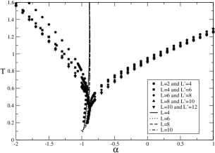
Figure 35: The phase diagram for $q=1.5$ found using transfer matrices and the phenomenological renormalization group with periodic (top) and free boundary conditions (bottom). The points correspond to finite-size estimates for $T_{c}$, whilst the lines correspond to the estimates for the disorder line, ($\alpha=J_{2}/J_{1}$) foster2 .

A frustrated checkerboard lattice with XY spins shows also evidence of a paramagnetic reentrance.Boubcheur

In vector spin models such as the Heisenberg and XY models, the frustration is shared by all bonds so that no free spins exist in the ground state. However, one can argue that if there are several kinds of local field in the ground state due to several kinds of interaction, then there is a possibility that a subsystem with weak local field is disordered at low $T$ while those of stronger local field stay ordered up to higher temperatures. This conjecture has been verified in a number of recent works on classicalSanta1 and quantum spinsSanta2 ; Quartu1 . Consider for example Heisenberg spins $\bf{S}_{i}$ on a bcc lattice with a unit cell shown in Fig. 36.Santa1

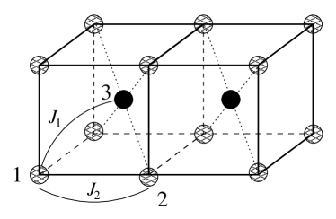
Figure 36: bcc lattice. Spins are shown by gray and black circles. Interaction between nn (spins numbered 1 and 3) is denoted by $J_{1}$ and that between nnn (spins 1 and 2) by $J_{2}$. Note that there is no interaction between black spins.

For convenience, let us call sublattice 1 the sublattice containing the sites at the cube centers and sublattice 2 the other sublattice. The Hamiltonian reads

$$\begin{array}[]{c}H=-\frac{1}{2}\sum_{<i,j>_{1}}{\bf S_{i}.S_{j}}-\frac{1}{2}\sum_{<i,j>_{2}}{\bf S_{i}.S_{j}\par}\end{array}$$

where $\sum_{<i,j>_{1}}$ indicates the sum over the nn spin pairs with exchange coupling $J_{1}$, while $\sum_{<i,j>_{2}}$ is limited to the nnn spin pairs belonging to sublattice 2 with exchange coupling $J_{2}$. It is easy to see that when $J_{2}$ is antiferromagnetic the spin configuration is non collinear for $J_{2}/|J_{1}|<-2/3$. In the non collinear case, one can verify that the local field acting a center spin (sublattice 1) is weaker in magnitude than that acting on a corner spin (sublattice 2). The partial disorder is observed in Fig. 37: the sublattice of black spins (sublattice 1) is disordered at a low $T$.

Figure 37: Monte Carlo results for sublattice magnetizations vs $T$ in the case $J_{1}=-1$, $J_{2}=-1.4$: black squares and black circles are for sublattices 1 and 2, respectively. Void circles indicate the total magnetization.

The same argument is applied for quantum spins.Quartu1 Consider the bcc crystal as shown in Fig. 36, but the sublattices are supposed now to have different spin magnitudes, for example $S_{A}=1/2$ (sublattice 1) and $S_{B}=1$ (sublattice 2). In addition, one can include nnn interactions in both sublattices, namely $J_{2A}$ and $J_{2B}$. The Green function technique is then applied for this quantum system.Quartu1 We show in Fig. 38 the partial disorder observed in two cases: sublattice 1 is disordered (Fig. 38a) or sublattice 2 is disordered (Fig. 38b). In each case, one can verify, using the corresponding parameters, that in the ground state the spin of the disordered sublattice has an energy lower than a spin in the other sublattice.

Figure 38: Sublattice magnetizations vs $T$ in the case $S_{A}=1/2$, $S_{B}=1$: (a) curve $a$ ($b$) is the sublattice-1(2) magnetization in the case $J_{2A}/|J_{1}|=0.2$ and $J_{2B}/|J_{1}|=0.9$ (b) curve $a$ ($b$) is the sublattice-1(2) magnetization in the case $J_{2A}/|J_{1}|=2.2$ and $J_{2B}/|J_{1}|=0.1$. P is the paramagnetic phase, PO the partial order phase (only one sublattice is ordered), II and III are non collinear spin configuration phases. See text for comments.

We show in Fig. 39 the specific heat versus $T$ for the parameters used in Fig. 38. One observes the two peaks corresponding to the two phase transitions associated with the loss of sublattice magnetizations.

Figure 39: Specific heat versus $T$ of the parameters used in Fig. 38, $S_{A}=1/2$, $S_{B}=1$: (a) $J_{2A}/|J_{1}|=0.2$ and $J_{2B}/|J_{1}|=0.9$ (b) $J_{2A}/|J_{1}|=2.2$ and $J_{2B}/|J_{1}|=0.1$. See the caption of Fig. 38 for the meaning of P, PO, II and III. See text for comments.

The necessary condition for the occurrence of a partial disorder at finite $T$ is thus the existence of several kinds of site with different energies in the ground state. This has been so far verified in a number of systems as shown above.

VI Conclusion

In this chapter, we have discussed some properties of periodically frustrated Ising systems. We have limited the discussion to exactly solved models which possess at least a reentrant phase. Other Ising systems which involved approximations are discussed in the chapter by Nagai et al (this book) and in the book by Liebmann.Lieb .

Let us emphasize that simple models having no bond disorder like those presented in this chapter can possess complicated phase diagrams due to the frustration generated by competing interactions. Many interesting physical phenomena such as successive phase transitions, disorder lines, and reentrance are found. In particular, a reentrant phase can occur in an infinite region of parameters. For a given set of interaction parameters in this region, successive phase transitions take place on the temperature scale, with one or two paramagnetic reentrant phases.

The relevance of disorder solutions for the reentrance phenomena has also been pointed out. An interesting finding is the occurrence of two disorder lines which divide the paramagnetic phase into regions of different kinds of fluctuations (section 4.2). Therefore, care should be taken in analyzing experimental data such as correlation functions, susceptibility, etc. in the paramagnetic phase of frustrated systems.

Although the reentrance is found in the models shown above by exact calculations, there is no theoretical explanation why such a phase can occur. In other words, what is the necessary and sufficient condition for the occurrence of a reentrance? We have conjecturedAza87 ; Diep92 that the necessary condition for a reentrance to take place is the existence of at least a partially disordered phase next to an ordered phase or another partially disordered phase in the ground state. The partial disorder is due to the competition between different interactions.

The existence of a partial disorder yields the occurrence of a reentrance in most of known cases,Vaks ; Mo ; Chi ; Aza87 ; Diep91b ; Diep92 except in some particular regions of interaction parameters in the centered honeycomb lattice (section 4.3.): the partial disorder alone is not sufficient to make a reentrance as shown in Fig. 27a and Fig. 27b, the finite zero-point entropy due to the partial disorder of the ground state is the same for three cases considered in Fig. 26 , i.e. $S_{0}=\log(2)/3$ per spin, but only one case yields a reentrance. Therefore, the existence of a partial disorder is a necessary, but not sufficient, condition for the occurrence of a reentrance.

The anisotropic character of the interactions can also favor the occurrence of the reentrance. For example, the reentrant region is enlarged by anisotropic interactions as in the centered square lattice,Chi and becomes infinite in the generalized Kagomé model (section 4.2.). But again, this alone cannot cause a reentrance as seen by comparing the anisotropic cases shown in Fig. 26b and Fig. 26c: only in the latter case a reentrance does occur. The presence of a reentrance may also require a coordination number at a disordered site large enough to influence the neighboring ordered sites. When it is too small such as in the case shown in Fig. 26b (equal to two), it cannot induce a reentrance. However, it may have an upper limit to avoid the disorder contamination of the whole system such as in the case shown in Fig. 27a where the coordination number is equal to six. So far, the ’right’ number is four in known reentrant systems shown above. Systematic investigations of all possible ingredients are therefore desirable to obtain a sufficient condition for the existence of a reentrance.

Finally, let us emphasize that when a phase transition occurs between states of different symmetries which have no special group-subgroup relation, it is generally accepted that the transition is of first order . However, the reentrance phenomenon is a symmetry breaking alternative which allows one ordered phase to change into another incompatible ordered phase by going through an intermediate reentrant phase. A question which naturally arises is under which circumstances does a system prefer an intermediate reentrant phase to a first-order transition. In order to analyze this aspect we have generalized the centered square lattice Ising model into three dimensions.Aza89b This is a special bcc lattice. We have found that at low $T$ the reentrant region observed in the centered square lattice shrinks into a first order transition line which is ended at a multicritical point from which two second order lines emerge forming a narrow reentrant region.Aza89b

As a final remark, let us mention that although the exactly solved systems shown in this chapter are models in statistical physics, we believe that the results obtained in this work have qualitative bearing on real frustrated magnetic systems. In view of the simplicity of these models, we believe that the results found here will have several applications in various areas of physics.

Note added for the third edition

There is a number of papers dealing with exactly solved frustrated models published by J. Strec̆ka and coworkers since 2006. These models are essentially decorated Ising models in one or two dimensions.

In Ref. [53] ground-state and finite-temperature properties of the mixed spin-1/2 and spin-S Ising-Heisenberg diamond chains are examined within an exact analytical approach based on the generalized decoration-iteration map. A particular emphasis is laid on the investigation of the effect of geometric frustration, which is generated by the competition between Heisenberg- and Ising-type exchange interactions. It is found that an interplay between the geometric frustration and quantum effects gives rise to several quantum ground states with entangled spin states in addition to some semi-classically ordered ones. Among the most interesting results to emerge from our study one could mention a rigorous evidence for quantized plateaux in magnetization curves, an appearance of the round minimum in the thermal dependence of susceptibility times temperature data, double-peak zero-field specific heat curves, or an enhanced magneto-caloric effect when the frustration comes into play. The triple-peak specific heat curve is also detected when applying small external field to the system driven by the frustration into the disordered state.

In Ref. [54], the geometric frustration of the spin-1/2 Ising-Heisenberg model on the triangulated kagomé ”triangles-in-triangles”lattice is investigated within the framework of an exact analytical method based on the generalized star-triangle mapping transformation. Ground-state and finite-temperature phase diagrams are obtained along with other exact results for the partition function, Helmholtz free energy, internal energy, entropy, and specific heat, by establishing a precise mapping relationship to the corresponding spin-1/2 Ising model on the kagomé lattice. It is shown that the residual entropy of the disordered spin liquid phase for the quantum Ising-Heisenberg model is significantly lower than for its semiclassical Ising limit ($S_{0}/NTk_{B}=0.2806$ and 0.4752, respectively), which implies that quantum fluctuations partially lift a macroscopic degeneracy of the ground-state manifold in the frustrated regime.

In Ref. [55], spin-1/2 Ising model with a spin-phonon coupling on decorated planar lattices partially amenable to lattice vibrations is examined using the decoration-iteration transformation and harmonic approximation. It is shown that the magneto-elastic coupling gives rise to an effective antiferromagnetic next-nearest-neighbor interaction, which competes with the nearest-neighbor interaction and is responsible for a frustration of decorating spins. A strong enough spin-phonon coupling consequently leads to an appearance of striking partially ordered and partially disordered phase, where a perfect antiferromagnetic alignment of nodal spins is accompanied with a complete disorder of decorating spins.

In the above works, the decorations are local couplings of an Ising spin to decorated Heisenberg spins or to phonons which can be summed up to renormalize the interactions between Ising spins. This leaves the systems solvable by star-triangle transformations, vertex models or other methods. Their results are interesting. We find again in these models striking features shown above in the present chapter for 2D solvable frustrated Ising models. In particular, partially disordered systems, multiple phase transitions and the reentrant phase due to the frustration are shown to exist in the phase diagrams.

For details, the reader is referred to Refs. [53,54,55].

References

- (1) R. Liebmann, Statistical Mechanics of Periodic Frustrated Ising Systems, Lecture Notes in Physics, vol. 251 (Springer-Verlag, Berlin, 1986).
- (2) G. Toulouse, Commun. Phys. 2, 115 (1977).
- (3) J. Villain, J. Phys. C10, 1717 (1977).
- (4) G. H. Wannier, Phys. Rev. 79, 357 (1950); Phys. Rev. B 7, 5017 (E) (1973).
- (5) A. Yoshimori, J. Phys. Soc. Jpn. 14, 807 (1959).
- (6) J. Villain, Phys. Chem. Solids 11, 303 (1959).
- (7) T. A. Kaplan, Phys. Rev. 116, 888 (1959).
- (8) B. Berge, H. T. Diep, A. Ghazali, and P. Lallemand, Phys. Rev. B 34, 3177 (1986).
- (9) P. Lallemand, H.T. Diep, A. Ghazali, and G. Toulouse, Physique Lett. 46, L-1087 (1985).
- (10) H. T. Diep, A. Ghazali and P. Lallemand, J. Phys. C18, 5881 (1985).
- (11) R. J. Baxter, Exactly solved Models in Statistical Mechanics (Academic, New York, 1982).
- (12) V. Vaks , A. Larkin and Y. Ovchinnikov, Sov. Phys. JEPT 22, 820 (1966).
- (13) T. Morita, J. Phys. A 19, 1701 (1987).
- (14) T. Chikyu and M. Suzuki, Prog. Theor. Phys. 78, 1242(1987).
- (15) K. Kano and S. Naya, Prog. Theor. Phys. 10, 158 (1953).
- (16) P. Azaria, H. T. Diep and H. Giacomini, Phys. Rev. Lett. 59, 1629 (1987).
- (17) M. Debauche, H.T. Diep, P. Azaria, and H. Giacomini, Phys. Rev. B 44, 2369 (1991).
- (18) H.T. Diep, M. Debauche and H. Giacomini, Phys. Rev. B 43, 8759 (1991).
- (19) M. Debauche and H. T. Diep, Phys. Rev. B 46, 8214 (1992); H. T. Diep, M. Debauche and H. Giacomini, J. of Mag. and Mag. Mater. 104, 184 (1992).
- (20) H. Kitatani, S. Miyashita and M. Suzuki, J. Phys. Soc. Jpn. 55 (1986) 865; Phys. Lett. A 158, 45 (1985).
- (21) T. Horiguchi, Physica A 146, 613 (1987).
- (22) J. Villain, R. Bidaux, J.P. Carton, and R. Conte, J. Physique 41, 1263 (1980).
- (23) T. Oguchi, H. Nishimori, and Y. Taguchi, J . Phys. Jpn. 54, 4494 (1985).
- (24) C. Henley, Phys. Rev. Lett. 62, 2056 (1989).
- (25) A. Gaff and J. Hijmann, Physica A 80, 149 (1975).
- (26) J. E. Sacco and F. Y. Wu, J. Phys. A 8, 1780 (1975).
- (27) J. Maillard , Second conference on Statistical Mechanics, California Davies (1986), unpublished.
- (28) K. Binder and A. P. Young, Rev. Mod. Phys. 58, 801 (1986).
- (29) T. Choy and R. Baxter, Phys. Lett. A 125, 365 (1987).
- (30) P. Azaria, H. T. Diep and H. Giacomini, Phys. Rev. B 39, 740 (1989).
- (31) D. Blankschtein, M. Ma and A. Berker, Phys. Rev. B 30, 1362 (1984).
- (32) H. T. Diep, P. Lallemand and O. Nagai, J. Phys. C 18, 1067 (1985).
- (33) J. Stephenson, J. Math. Phys. 11, 420 (1970); Can. J. Phys. 48, 2118 (1970); Phys. Rev. B 1, 4405 (1970) .
- (34) F. Y. Wu and K.Y. Lin , J. Phys. A 20, 5737 (1987).
- (35) H. Giacomini , J. Phys. A 19, L335 (1986) .
- (36) R. Baxter , Proc. R. Soc. A 404, 1 (1986).
- (37) P. Rujan , J. Stat. Phys. 49, 139 (1987) .
- (38) M. Suzuki and M. Fisher, J. Math. Phys. 12, 235 (1971).
- (39) F. Y. Wu, Solid Stat. Comm. 10, 115 (1972) .
- (40) L. Onsager, Phys. Rev. 65, 117 (1944).
- (41) C. S. Hsue, K. Y. Lin, and F.Y. Wu, Phys. Rev. B 12, 429 (1975).
- (42) K. Y. Lin and I. P. Wang, J. Phys. A 10, 813 (1977).
- (43) J. Imbrie, Phys. Rev. Lett. 53, 1747 (1984).
- (44) D. Blankschtein, M. Ma , A. Nihat Berker, G. S. Grest, and C. M. Soukoulis, Phys. Rev. B 29, 5250 (1984).
- (45) See the chapter by O. Nagai, T. Horiguchi and S. Miyashita, this book.
- (46) P. Azaria, H. T. Diep and H. Giacomini, Europhys. Lett. 9, 755 (1989).
- (47) D.P. Foster, C. Gérard and I. Puha, J. Phys. A: Math. Gen. 34, 5183 (2001).
- (48) D.P. Foster and C. Gérard, Phys. Rev. B to appear (2004).
- (49) E. H. Boubcheur, R. Quartu, H. T. Diep and O. Nagai, Phys. Rev. B 58, 400 (1998).
- (50) C. Santamaria and H. T. Diep, J. Appl. Phys. 81, 5276 (1997).
- (51) C. Santamaria, R. Quartu and H. T. Diep, J. Appl. Phys. 84, 1953 (1998).
- (52) R. Quartu and H. T. Diep, Phys. Rev. B 55, 2975 (1997).
- (53) L. C̆anová, J. Strec̆ka, M. Jas̆c̆ur, Geometric frustration in the class of exactly solvable Ising-Heisenberg diamond chains, J. Phys.: Condens. Matter 18, 4967-4984 (2006).
- (54) J. Strec̆ka, L. C̆anová, M. Jas̆c̆ur, M. Hagiwara, Exact solution of the geometrically frustrated spin-1/2 Ising-Heisenberg model on the triangulated (triangles-in-triangles) lattice, Phys. Rev. B 78, 024427 (2008).
- (55) J. Strec̆ka, Onofre Rojas, S. M. de Souza, Spin-phonon coupling induced frustration in the exactly solved spin-1/2 Ising model on a decorated planar lattice, Phys. Lett. A 376,197-202 (2012).