Acoustic radiation torque exerted on a subwavelength spheroidal particle by a traveling and standing plane wave

Abstract

The nonlinear interaction of ultrasonic waves with a nonspherical particle may give rise to the acoustic radiation torque on the particle. This phenomenon is investigated here considering a rigid prolate spheroidal particle of subwavelength dimensions that is much smaller than the wavelength. Using the partial wave expansion in spheroidal coordinates, the radiation torque of a traveling and standing plane wave with arbitrary orientation is exactly derived in the dipole approximation. We obtain asymptotic expressions of the torque as the particle geometry approaches a sphere and a straight line. As the particle is trapped in a pressure node of a standing plane wave, its radiation torque equals that of a traveling plane wave. We also find how the torque changes with the particle aspect ratio. Our findings are in excellent agreement with previous numerical computations. Also, by analyzing the torque potential energy, we determine the stable and unstable spatial configuration available for a particle.

I Introduction

There has been an increasing interest in studying the ultrasonic patterning of nonspherical particles such as fibers Brodeur1990 ; Yamahira2000 , microrods Saito1998 , nanorods Wang2012 , microfibers Schwarz2015 , and stretched droplets Foresti2013 . These particles are translated by the action of the acoustic radiation force Silva2014 and may change orientation due to the acoustic radiation torque. Physically, this torque corresponds to the moment of the radiation stress on a particle Zhang2011c .

A typical example of the acoustic radiation torque phenomenon on a nonspherical particle is the Rayleigh disk placed obliquely to the wave propagation direction Rayleigh1945 . Kotani Kotani1933 analyzed the radiation torque on a Rayleigh disk caused by a traveling wave using oblate spheroidal wave functions. King King1935 used a cylindrical wave function basis to calculate the radiation torque due to a standing plane wave. Keller Keller1957 obtained the radiation torque on infinitely long strips and disks employing the Babinet’s principle. Based on the angular momentum flux conservation, Maidanik Maidanik1958 proposed a farfield calculation method and derived a solution for disks.

Radiation torque solutions involving spheroidal particles are more scarce. Some numerical methods have been employed to study this problem. The boundary element method (BEM) was utilized to calculate the torque exerted by a standing wave on a rigid spheroidal particle Wijaya2015 . The Born approximation with numerical quadrature was used to obtain the radiation torque on a compressible spheroidal particle, with density and compressibility close to those of the surrounding fluid.Jerome2019 To date, the only analytical result to this problem was presented by Fan et al. Fan2008 . However, this investigation is mainly focused on developing a general theoretical framework for arbitrarily shaped particles in the long-wavelength limit.

In this paper, we present the analytical solution of the radiation torque caused by a traveling and standing plane wave on a subwavelength spheroidal particle. The incident waves may have arbitrary orientation regarding the particle major axis. We obtain the radiation torque in the inviscid limit solving the corresponding scattering problem in spheroidal coordinates. The result is used in Maidanik’s farfield method Maidanik1958 . The inviscid approximation is useful when the depth of the viscous boundary layer is much smaller than the particle size and streaming is weak. We derive simple asymptotic expressions as the particle geometry approaches a sphere and straight line. Excellent agreement is found between our method and BEM results considering a subwavelength prolate spheroid in a standing wave field Wijaya2015 .

II Acoustic scattering

Consider an inviscid fluid with density $\rho_{0}$, speed of sound $c_{0}$, and compressibility $\beta_{0}=1/\rho_{0}c_{0}^{2}$. A spheroidal particle with a major and minor axis denoted by $2a$ and $2b$, respectively, is centered at the origin of the coordinate system–see Fig. 1. The particle interfocal distance is $d=2\sqrt{a^{2}-b^{2}}$.

A traveling or standing plane wave of angular frequency $\omega$ and wavenumber $k=2\pi/\lambda$, with $\lambda$ being the wavelength, is scattered by the particle. For symmetry reasons, the acoustic scattering will be described in prolate spheroidal coordinates. The Cartesian-to-spheroidal coordinate relations are

$$x =\frac{d}{2}\sqrt{(\xi^{2}-1)(1-\eta^{2})}\cos\varphi,$$ (1a)

$$y =\frac{d}{2}\sqrt{(\xi^{2}-1)(1-\eta^{2})}\sin\varphi,$$ (1b)

$$z =\frac{d\xi\eta}{2},$$ (1c)

where $\xi\geq 1$ is radial distance, $-1\leq\eta\leq 1$, and $0\leq\varphi\leq 2\pi$ is azimuth angle. A prolate spheroidal particle corresponds to $\xi=\xi_{0}=2a/d$. The aspect ratio of the particle is ${a}/{b}=(1-\xi_{0}^{-2})^{-1/2}$, while its volume is expressed by $V=4\pi ab^{2}/3=\pi d^{3}\xi_{0}(\xi_{0}^{2}-1)/6.$

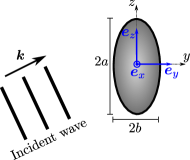
Figure 1: (color online) An incident wave with arbitrary wavevector $\bm{k}$ interacts with a prolate spheroid of major and minor axis denoted by $2a$ and $2b$, respectively. The origin of the Cartesian coordinate system is placed in the geometric center of the particle. The unit-vectors of the coordinate system are $\bm{e}_{x}$, $\bm{e}_{y}$, and $\bm{e}_{z}$.

In the subwavelength scattering analysis, it is useful to define an expansion parameter in terms of the interfocal-to-wavelength ratio as

$$\epsilon=\frac{kd}{2}\ll 1.$$ (2)

In this limit, only the monopole and dipole modes of the incident and scattered waves are needed to describe the particle-wave interaction. Accordingly, the partial wave expansions of the incident and scattering potential velocities are given in prolate spheroidal coordinates by Flammer2005

$$\phi_{\text{in}} =\phi_{0}\sum_{n=0}^{1}\sum_{m=-n}^{n}a_{nm}S_{nm}(\epsilon,\eta)R_{nm}^{(1)}(\epsilon,\xi)\textrm{e}^{\textrm{i}m\varphi},$$ (3a)

$$\phi_{\text{sc}} =\phi_{0}\sum_{n=0}^{1}\sum_{m=-n}^{n}a_{nm}s_{nm}S_{nm}(\epsilon,\eta)R_{nm}^{(3)}(\epsilon,\xi)\textrm{e}^{\textrm{i}m\varphi},$$ (3b)

where $S_{nm}$ is the angular function of the first kind, and $R_{nm}^{(1)}$ and $R_{nm}^{(3)}$ are the radial functions of the first and third kind, respectively. The quantities $a_{nm}$ and $s_{nm}$ are the beam-shape and scaled scattering coefficients.

Assuming that the particle behaves as a rigid and immovable spheroid, the normal component of fluid velocity on the particle surface satisfies $v_{\xi}(\xi_{0})=\partial_{\xi}(\phi_{\textrm{in}}+\phi_{\textrm{sc}})_{\xi=\xi_{0}}=0$. Using this condition into (3) yields the scattering coefficient as

$$s_{nm}=-\frac{\partial_{\xi}R_{nm}^{(1)}}{\partial_{\xi}R_{nm}^{(3)}}\biggr{|}_{\xi=\xi_{0}}.$$ (4)

We shall see later that the acoustic radiation torque depends on the dipole moment ($n=1$) of the incident and scattered waves. After Taylor-expanding the radial functions as given in (25) around $\epsilon=0$ and use the result into (4), we obtain the dipole scattering coefficients as Silva2018

$$s_{10} =\frac{\textrm{i}\epsilon^{3}}{6}f_{10}-\frac{\epsilon^{6}}{36}f_{10}^{2},$$ (5a)

$$s_{1,-1} =s_{11}=\frac{\textrm{i}\epsilon^{3}}{12}f_{11}-\frac{\epsilon^{6}}{144}f_{11}^{2},$$ (5b)

where

$$f_{10} =\frac{2}{3}\left[\frac{\xi_{0}}{\xi_{0}^{2}-1}-\ln\left(\frac{\xi_{0}+1}{\sqrt{\xi_{0}^{2}-1}}\right)\right]^{-1},$$ (6a)

$$f_{11} =\frac{8}{3}\left[\frac{2-\xi_{0}^{2}}{\xi_{0}(\xi_{0}^{2}-1)}+\ln\left(\frac{\xi_{0}+1}{\sqrt{\xi_{0}^{2}-1}}\right)\right]^{-1}$$ (6b)

are the scattering factors.

In the farfield $k\xi\gg 1$, the spheroidal wave functions in (3) become spherical wave functions expressed in spherical coordinates $(r,\theta,\varphi)$ as follows Silva2018

$$\phi_{\textrm{in}} =\frac{\phi_{0}}{kr}\sum_{n=0}^{1}\sum_{m=-n}^{n}{a}_{nm}\sin\left(kr-\frac{n\pi}{2}\right)Y_{n}^{m}(\theta,\varphi),$$ (7a)

$$\phi_{\textrm{sc}} =\phi_{0}\frac{\textrm{e}^{\textrm{i}kr}}{kr}\sum_{n=0}^{1}\sum_{m=-n}^{n}\textrm{i}^{-n-1}{a}_{nm}s_{nm}Y_{n}^{m}(\theta,\varphi),$$ (7b)

where $Y_{n}^{m}(\theta,\varphi)$ is the spherical harmonic of $n$th-order and $m$th-degree. Here the coefficient $a_{nm}$ describes an incident wave in spherical coordinates. Some analytic expressions of beam-shape coefficients include Bessel vortex and Gaussian beams Mitri2014 . Numerical schemes and the addition theorem of spherical functions can be used to compute these coefficients for different types of beams Silva2011a ; Mitri2011 ; Silva2015a ; Silva2013 ; Lopes2016 .

III Acoustic radiation torque

The density of linear momentum flux conveyed by an acoustic wave is given by Silva2011 $\overline{\bf{P}}=-\overline{\mathcal{L}}{\bf I}+\rho_{0}\overline{\bm{v}\bm{v}}$, with the over bar denoting time-average over a wave period, and $\bf I$ being the unit tensor. The fields $\mathcal{L}$ and $\rho_{0}\bm{v}\bm{v}$ are the Lagrangian density and Reynolds’ stress (a linear momentum flux). The density of angular momentum flux is defined as $\overline{\bf{L}}=\bm{r}\times\overline{\bf{P}}=\bm{r}\times\rho_{0}\overline{\bm{v}\bm{v}}$, since $\bm{r}\times\bf{I}=\bm{0}$. The acoustic radiation torque on a particle with surface $S_{0}$ is expressed by

$$\bm{\tau}_{\text{rad}}=\int_{S_{0}}\overline{\bf{L}}\cdot\bm{n}\,\textrm{d}S=\int_{S_{0}}\left(\bm{r}\times\rho_{0}\overline{\bm{v}\bm{v}}\right)\cdot\bm{n}\,\textrm{d}S.$$ (8)

The angular momentum flux satisfies the conservation law Zhang2011c $\nabla\cdot\overline{\bf{L}}=\bm{0}$. Thus, the integral in Eq. (8) can be evaluated over a farfield virtual surface $S$ that encloses the particle. Accordingly, the radiation force is expressed by Maidanik1958 $\bm{\tau}_{\text{rad}}=-\int_{S}\left(\bm{r}\times\rho_{0}\overline{\bm{v}\bm{v}}\right)\cdot\bm{n}\,\textrm{d}S.$

The fluid velocity is the sum of the velocity from the incident and scattered waves, $\bm{v}=\bm{v}_{\text{in}}+\bm{v}_{\text{sc}}$. Using this expression into the farfield radiation torque and noting that $\overline{\bm{v}\bm{v}}=(1/2)\text{Re}[\bm{v}\bm{v}^{*}]$, we arrive at

$$\bm{\tau}_{\text{rad}}=-\frac{\rho_{0}r^{2}}{2}\text{Re}\int_{\Omega_{\text{s}}}\bm{r}\times(\bm{v}_{\text{in}}\bm{v}_{\text{sc}}^{*}+\bm{v}_{\text{sc}}\bm{v}_{\text{in}}^{*}+\bm{v}_{\text{sc}}\bm{v}_{\text{sc}}^{*})\cdot\bm{e}_{r}\,\textrm{d}\Omega_{\text{s}},$$ (9)

where ‘Re’ means the real part of, asterisk denotes complex conjugation, and $\Omega_{\text{s}}$ represents the unit-sphere. In the inviscid approximation, no torque is formed in the fluid without a particle; hence, $\text{Re}\int_{\Omega_{\text{s}}}\bm{r}\times\bm{v}_{\text{in}}\bm{v}_{\text{in}}^{*}\cdot\bm{e}_{r}\,\textrm{d}\Omega_{\text{s}}=\bm{0}$. Replacing the velocity potentials in (7) into Eq. (9), we find the radiation torque to the dipole approximation as Silva2012

$${\tau}_{\text{rad},x} =-\frac{E_{0}}{k^{3}\sqrt{2}}\,\text{Re}\biggl{[}(a_{1,-1}+a_{11})(1+s_{11})a^{*}_{10}s^{*}_{10}$$

$$+a_{10}(1+s_{10})(a_{1,-1}^{*}+a_{11}^{*})s_{11}^{*}\biggr{]},$$ (10a)

$${\tau}_{\text{rad},y} =\frac{E_{0}}{k^{3}\sqrt{2}}\,\text{Re}\biggl{[}\textrm{i}\,(a_{1,-1}-a_{11})(1+s_{11})a^{*}_{10}s^{*}_{10}$$

$$-\textrm{i}\,a_{10}(1+s_{10})(a_{1,-1}^{*}-a_{11}^{*})s_{11}^{*}\biggr{]},$$ (10b)

$${\tau}_{\text{rad},z} =\frac{E_{0}}{k^{3}}\,\text{Re}\left[(|a_{1,-1}|^{2}-|a_{11}|^{2})(1+s_{11})s_{11}^{*}\right],$$ (10c)

where $E_{0}=\rho_{0}k^{2}\phi_{0}/2$ is the characteristic energy density of the incident wave, with $p_{0}$ being its peak pressure.

IV Plane wave examples

IV.1 Traveling plane wave

The velocity potential of a traveling plane wave (TPW) propagating in an arbitrary direction is

$$\phi_{\textrm{in}}=\phi_{0}\,\textrm{e}^{\textrm{i}{\bm{k}}\cdot{\bm{r}}}.$$ (11)

The wavevector reads

$${\bm{k}} =k\bm{e}_{k}$$

$$=k\left(\sin\theta_{k}\cos\varphi_{k}\,{\bm{e}}_{x}+\sin\theta_{k}\sin\varphi_{k}\,{\bm{e}}_{y}+\cos\theta_{k}\,{\bm{e}}_{z}\right).$$ (12)

The angles $\theta_{k}$ and $\varphi_{k}$ are polar and azimuthal angles of the wave propagation direction. Note that the orientation of the spheroidal particle is fixed along the direction determined by the unit-vector $\bm{e}_{z}$. The orientation angle regarding the wave propagation direction $\bm{e}_{k}$ is determined from $\cos\theta_{k}=\bm{e}_{k}\cdot\bm{e}_{z}$.

The beam-shape coefficient is obtained from the TPW partial wave expansion in spherical coordinates

$$\textrm{e}^{\textrm{i}\bm{k}\cdot\bm{r}}=4\pi\sum_{n,m}\textrm{i}^{n}Y_{n}^{m*}(\theta_{k},\varphi_{k})\,j_{n}(kr)Y_{n}^{m}(\theta,\varphi).$$ (13)

Thus,

$${a}_{nm}=4\pi\textrm{i}^{n}Y_{n}^{m*}(\theta_{k},\varphi_{k}).$$ (14)

Replacing this coefficient into (10) and noting that $s_{1,-1}=s_{11}$, we obtain

$$\bm{\tau}_{\text{rad}}^{\text{T}}=\frac{12\pi E_{0}}{k^{3}}\text{Im}\left[s_{10}^{*}+s_{11}+2s_{10}^{*}s_{11}\right](\bm{e}_{k}\cdot\bm{e}_{z})\left(\bm{e}_{k}\times\bm{e}_{z}\right),$$ (15)

where we have used $\sin\theta_{k}\,(\sin\varphi_{k}\,\bm{e}_{x}-\cos\varphi_{k}\,\bm{e}_{y})=(\bm{e}_{k}\times\bm{e}_{z})$. Inserting the scattering coefficient given in (5) into Eq. (15) and noting that $\epsilon^{3}=3k^{3}V/[4\pi\xi_{0}(\xi_{0}^{2}-1)]$, we find the radiation torque as

$$\bm{\tau}^{\text{T}}_{\text{rad}} =VE_{0}Q_{\text{rad}}\left(\bm{e}_{k}\cdot\bm{e}_{z}\right)\left(\bm{e}_{k}\times\bm{e}_{z}\right),$$ (16a)

$$Q_{\text{rad}} =\frac{3}{4}\frac{f_{11}-2f_{10}}{\xi_{0}(\xi_{0}^{2}-1)},$$ (16b)

where $Q_{\text{rad}}$ is the radiation torque efficiency. It is useful to define the characteristic radiation torque as $\tau_{0}=VE_{0}Q_{\text{rad}}$.

In the dipole approximation, the radiation torque does not involve self-interaction of the scattered wave. The torque is caused by the interference terms of the momentum flux $\rho_{0}\bm{v}_{\text{in}}\bm{v}_{\text{sc}}^{*}$ and $\rho_{0}\bm{v}_{\text{sc}}\bm{v}_{\text{in}}^{*}$.

Due to the axial symmetry of the particle, no radiation torque is produced with end-on incidence ($\theta_{k}=0,\pi$). It also vanishes in broadside incidence ($\theta_{k}=\pi/2$). The maximum radiation torque is reached as $\theta_{k}=\pi/4$. We also note that the radiation torque does not depend on frequency.

We may expand the torque efficiency in Eq. (16b) as the particle geometry approaches a sphere ($\xi_{0}\rightarrow\infty$),

$$Q_{\text{rad}}=\frac{9}{20}\left(\frac{1}{\xi_{0}^{2}}+\frac{23}{70\xi_{0}^{4}}\right).$$ (17)

The radiation torque vanishes for a spherical particle, $\lim_{\xi_{0}\rightarrow\infty}{Q}_{\text{rad}}={0}$. This result is in agreement with the fact that no radiation torque is produced on a rigid sphere Silva2012 .

The expansion of $Q_{\text{rad}}$ around $\xi_{0}=1$ gives the radiation torque on a straight line. Accordingly, we have

$$Q_{\text{rad}}=1+3(\xi_{0}-1)\left[2+\ln\left(\frac{\xi_{0}-1}{2}\right)\right].$$ (18)

For $\xi_{0}=1$, the radiation torque efficiency becomes $Q_{\text{rad}}=1$.

IV.2 Standing plane wave

Consider a standing plane wave (SPW) formed by the superposition of two counter-propagating traveling plane waves. The incident wave function is expressed by

$$\phi_{\textrm{in}} =\phi_{0}\cos\left[\bm{k}\cdot(\bm{r}+\bm{r}_{\textrm{0}})\right]$$

$$=\phi_{0}\left[\textrm{e}^{\textrm{i}\bm{k}\cdot(\bm{r}+\bm{r}_{\textrm{0}})}+\textrm{e}^{-\textrm{i}\bm{k}\cdot(\bm{r}+\bm{r}_{\textrm{0}})}\right],$$ (19)

where $\bm{r}_{0}$ points from the particle center to the nearest pressure antinode, which lies in the same direction as the wavevector, $\bm{k}\cdot\bm{r}_{0}=kr_{0}$.

To obtain the beam-shape coefficient of the SPW, we use the TPW expansion from Eq. (13) into Eq. (19) with the spherical harmonic relation $Y_{n}^{m*}=(-1)^{m}Y_{n}^{-m}$. Hence,

$${a}_{nm}=4\pi\cos\left(kr_{0}+\frac{n\pi}{2}\right)Y_{n}^{m*}(\theta_{k},\varphi_{k}).$$ (20)

Substituting this coefficient into the radiation torque components in (10) yields

$$\bm{\tau}_{\text{rad}}^{\text{S}} =\frac{12\pi E_{0}}{k^{3}}\text{Im}\left[s_{10}^{*}+s_{11}+2s_{10}^{*}s_{11}\right]$$

$$\times\sin^{2}kr_{0}\,(\bm{e}_{k}\cdot\bm{e}_{z})\left(\bm{e}_{k}\times\bm{e}_{z}\right).$$ (21)

Referring to Eq. (16a), the relation between the radiation torque of a standing and traveling plane wave is given by

$$\bm{\tau}_{\text{rad}}^{\text{S}}=\sin^{2}kr_{0}\,\bm{\tau}_{\text{rad}}^{\text{T}}.$$ (22)

We note that Eqs. (16b), (17), and (18) are valid for a standing plane wave.

Due to the acoustic radiation force Silva2018 , the spheroidal particle has a tendency to be trapped in a pressure node $kr_{0}=\pi/2$. At the trapping point, the radiation torque of a standing plane wave is tantamount that of a traveling plane wave, $\bm{\tau}_{\text{rad}}^{\text{S}}=\bm{\tau}_{\text{rad}}^{\text{T}}.$

In Fig. 2, we depict a spheroidal particle under the influence of the radiation torque of a SPW. Panel (a) and (b) shows the SPW with the wavevectors $\bm{k}=k(\sin\theta_{k}\,\bm{e}_{y}+\cos\theta_{k}\,\bm{e}_{z})$ in the $yz$-plane and $\bm{k}=k(\sin\theta_{k}\,\bm{e}_{x}+\cos\theta_{k}\,\bm{e}_{z})$ in the $xz$-plane, respectively. The corresponding radiation torques are $\bm{\tau}^{\text{S}}_{\text{rad}}=(\tau_{0}/2)\sin 2\theta_{k}\,\bm{e}_{x}$ and $\bm{\tau}^{\text{S}}_{\text{rad}}=(\tau_{0}/2)\sin 2\theta_{k}\,(-\bm{e}_{y}).$ Both torques set the particle to oscillate around $\theta_{k}=\pi/2$, e.g., at right angle with the wave propagation direction.

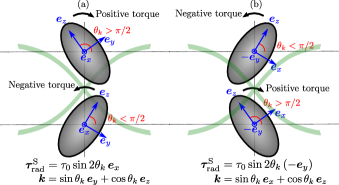
Figure 2: (color online) The radiation torque due to a standing plane wave (light green line) with wavevector in (a) the $xz$ plane and (b) the $yz$ plane. In both cases, the radiation torque is positive as $\theta_{k}<\pi/2$, and negative as $\theta_{k}>\pi/2$.

In Fig. 3, we compared the theoretical results with numerical simulation data from the boundary element method (BEM) Wijaya2015 . We consider the radiation torque efficiency $Q_{\text{rad}}$ times $\sin 2\theta_{k}$ of a standing plane wave and particles with different aspect ratios, $a/b=1.2$, $1.5$, $2.0$. The efficiency is compared with the dimensionless torque $T_{\text{st}}$ shown in (Wijaya2015, , Fig. 6b). By direct inspection, we find that $Q_{\text{rad}}\sin 2\theta_{k}=4T_{\text{st}}/k^{3}V$, where $k^{3}V=0.00103745$. Excellent agreement is found between our result and numerical data. In the inset, we note that the efficiency $Q_{\text{rad}}$ monotonically decreases with the radial parameter $\xi_{0}$ as it approaches to a spherical shape.

V Torque potential energy

Moving on now to consider the potential energy of the radiation torque of a particle at a pressure node of a standing plane wave. This also corresponds to the case of a traveling plane wave. Assume that the radiation torque corresponds to the situation described in Fig. 2, panel (a). The work done by the radiation torque from $\pi/2$ to an angle $\theta_{k}$ is

$$W=\int_{\pi/2}^{\theta_{k}}\tau^{\text{S,T}}_{\text{rad}}(\theta)\,\textrm{d}\theta=-\frac{\tau_{0}}{2}\cos^{2}\theta_{k}=-\frac{\tau_{0}}{2}\left(\bm{e}_{k}\cdot\bm{e}_{z}\right)^{2}.$$ (23)

Therefore, the potential energy variation associated the radiation torque is given by

$$\Delta U=U(\theta_{k})-U(\pi/2)=-W=\frac{\tau_{0}}{2}\left(\bm{e}_{k}\cdot\bm{e}_{z}\right)^{2}.$$ (24)

The minimum of the potential energy is $U(\pi/2)=0$, which shows the particle major axis has a tendency to set itself broadside ($\theta_{k}=\pi/2$) on to the direction of the propagation of incident plane waves. On the other hand, if the incidence angle is $\theta_{k}=0$, the potential energy is maximum $U(0)=\tau_{0}/2$, which corresponds to an unstable equilibrium point. This result agrees with experimental observations of polystyrene fibers Yamahira2000 and microrods Saito1998 that are trapped in a pressure node of standing wave field. These particles form a pattern in parallel alignment with the nodal planes.

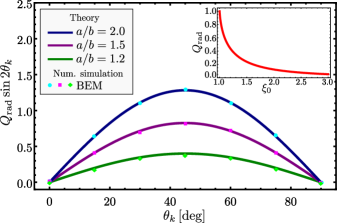
Figure 3: (color online) The radiation torque efficiency $Q_{\text{rad}}$ times $\sin 2\theta_{k}$ (solid lines) versus the incident angle $\theta_{k}$. The theoretical result is compared with numerical simulation data considering particles with different aspect ratios. The data is obtained with the boundary element method (BEM) Wijaya2015 . The inset shows $Q_{\text{rad}}$ as a function of the radial parameter $\xi_{0}$.

VI Discussion and conclusion

We have presented analytic expressions of the acoustic radiation torque caused by a traveling and standing plane wave on a subwavelength spheroidal particle. The results are exact to the dipole approximation of the acoustic field expansions. We found that the radiation torque is caused by interference between the incident and scattered waves. Simple expressions of the asymptotic radiation torque as the particle geometry approaches a sphere and straight-line have also been derived. The torque decreases monotonically as the particle assumes a spherical geometry.

When a particle is trapped in a pressure node of a standing wave, the radiation torque is the same as that of a traveling plane wave. The peak radiation torque occurs as the wave incidence angle is $\theta_{k}=\pi/4$. The potential energy associated with the radiation torque reveals that the particle equilibrium orientation is broadside on ($\theta_{k}=\pi/2$) to the wave propagation direction. Whereas, end-on incidence ($\theta_{k}=0$) promotes an unstable orientation setting the particle rotate toward the equilibrium orientation position ($\theta_{k}=\pi/2$).

The stable configuration predicted here agrees with previous experimental observation of fibers and microrods that are much smaller than the wavelength Yamahira2000 ; Saito1998 . Moreover, our findings are in excellent agreement with numerical simulation results based on the boundary element method Wijaya2015 . Finally, our results can be used to better analyze the dynamics of elongated cells and microorganisms (of prolate spheroidal shape) in acoustofluidic devices and of reinforcing fibers in layered structures and in composite materials.

Appendix A Monopole and dipole radial functions

In the long-wavelength approximation $\epsilon\ll 1$, the radial spheroidal functions can be expressed by Burke1966

$$R_{00}^{(1)} =1+\frac{\epsilon^{2}}{18}\left(2-3C_{1}^{2}\right)+\frac{\epsilon^{4}}{16200}\biggl{[}112-180C_{1}^{2}+135C_{1}^{4}+\frac{\epsilon^{2}}{882}\left(2192-8064C_{1}^{2}+5670C_{1}^{4}-2835C_{1}^{6}\right)\biggr{]},$$ (25a)

$$R_{10}^{(1)} =\frac{\epsilon}{C_{1}}+\frac{\epsilon^{2}C_{1}}{150}\biggl{[}2-5C_{1}^{2}+\frac{\epsilon^{2}}{4900}\left(368-700C_{1}^{2}+875C_{1}^{4}\right)\biggr{]},$$ (25b)

$$R_{11}^{(1)} =\frac{\epsilon S_{1}}{3}+\frac{\epsilon^{3}S_{1}}{150}\biggl{[}4-5C_{1}^{2}+\frac{\epsilon^{2}}{4900}(712-1400C_{1}^{2}+875C_{1}^{4})\biggr{]},$$ (25c)

$$R_{00}^{(2)} =-\frac{2}{\epsilon}\biggl{\{}L-\frac{\epsilon^{2}}{6}[6C_{1}+L(3C_{2}-5)]+\frac{3}{5}\left(\frac{\epsilon}{6}\right)^{4}\left[11C_{1}+9C_{3}+\frac{L}{60}(1109-1380C_{2}+135C_{4})\right]\biggr{\}},$$ (25d)

$$R_{10}^{(2)} =\frac{3C_{1}}{\epsilon^{2}}\biggl{\{}2C_{1}-\frac{C_{2}}{C_{1}}-2L-\left(\frac{\epsilon}{10}\right)^{2}\left[18C_{1}-\frac{4C_{2}}{C_{1}}+L(22-10C_{2})\right]+\frac{1}{882}\left(\frac{\epsilon}{10}\right)^{4}$$

$$\times\biggl{[}272313C1-864\frac{C_{2}}{C_{1}}+7875C_{3}-L(116073-99540C_{2}+7875C_{2})\biggr{]}\biggr{\}},$$ (25e)

$$R_{11}^{(2)} =-\frac{3S_{1}}{2\epsilon^{2}}\biggl{\{}\frac{C_{1}}{S_{1}^{2}}-2L-\left(\frac{\epsilon}{10}\right)^{4}\biggl{[}8C_{1}\left(5-\frac{1}{S_{1}^{2}}\right)-8L(33+5C_{2})\biggr{]}-\frac{1}{196}\left(\frac{\epsilon}{10}\right)^{2}\biggl{[}85800C_{1}-1750C_{3}$$

$$+\frac{712C_{1}}{S_{1}^{2}}-L(106324-76950C_{2}-1750C_{4})\biggr{]}\biggr{\}},$$ (25f)

$$R_{nm}^{(3)} =R_{nm}^{(1)}+\textrm{i}R_{nm}^{(2)},$$ (25g)

where $R_{nm}^{(2)}$ is the radial function of the second-kind. We note that $R_{nm}^{(i)}=R^{(i)}_{n,-m}$, with $i=1,2,3$. We also have

$$C_{n} =\frac{1}{2}\left[(\sqrt{\xi^{2}-1}+\xi)^{n}+(\sqrt{\xi^{2}-1}+\xi)^{-n}\right],$$

$$S_{n} =\frac{1}{2}\left[(\sqrt{\xi^{2}-1}+\xi)^{n}-(\sqrt{\xi^{2}-1}+\xi)^{-n}\right],$$

$$L =\frac{1}{2}\ln\left(\frac{1+(\sqrt{\xi^{2}-1}+\xi)^{-1}}{1-(\sqrt{\xi^{2}-1}+\xi)^{-1}}\right).$$

References

• (1) P. Brodeur, “Motion of fluid-suspended wave field,” Ultrasonics 29, 302–307 (1990).
• (2) S. Yamahira, S.-I. Hanaka, M. Kuwabara, and S. Asai, “Orientation of fibers in liquid by ultrasonic standing waves,” Jpn. J. Appl. Phys. 39, 3683 (2000).
• (3) M. Saito, T. Daian, K. Hayashi, and S.-Y. Izumida, “Fabrication of a polymer composite with periodic structure by the use of ultrasonic waves,” J. Appl. Phys. 83, 3490–3494 (1998).
• (4) W. Wang, L. A. Castro, M. Hoyos, and T. E. Mallouk, “Autonomous motion of metallic microrods propelled by ultrasound,” ACS Nano 67, 6122–6132 (2012).
• (5) T. Schwarz, P. Hahn, G. Petit-Pierre, and J. Dual, “Rotation of fibers and other non-spherical particles by the acoustic radiation torque,” Microfluid Nanofluid 18, 65 (2015).
• (6) D. Foresti and D. Poulikakos, “Acoustophoretic contactless elevation, orbital transport and spinning of matter in air,” Phys. Rev. Lett. 112, 024301 (2014).
• (7) G. T. Silva, “Acoustic radiation force and torque on an absorbing compressible particle in an inviscid fluid,” J. Acoust. Soc. Am. 136, 2405–2413 (2014).
• (8) L. Zhang and P. L. Marston, “Acoustic radiation torque and the conservation of angular momentum (L),” J. Acoust. Soc. Am. 129(4), 1679–1680 (2011).
• (9) J. W. S. Rayleigh, The Theory Of Sound, Vol. 2 (Dover Publications, 1945).
• (10) M. Kotani, “An acoustical problem relating to the theory of Rayleigh disc,” Proc. Phys. Math. Soc. Japan 15, 30 (1933).
• (11) L. V. King, “On the theory of the inertia and diffraction corrections for the Rayleigh disc,” Proc. Royal Soc. A 153, 17 (1935).
• (12) J. B. Keller, “Acoustic torques and forces on disks,” J. Acoust. Soc. Am. 29, 1085 (1957).
• (13) G. Maidanik, “Torques due to acoustical radiation pressure,” J. Acoust. Soc. Am. 30, 620–623 (1958).
• (14) F. B. Wijaya and K.-M. Lim, “Numerical calculation of acoustic radiation force and torque acting on rigid non-spherical particles,” Acta Acust. united Ac. 101, 531 (2015).
• (15) T. S. Jerome, Y. A. Ilinskii, E. A. Zabolotskaya, and M. F. Hamilton, “Born approximation of acoustic radiation force and torque on soft objects of arbitrary shape,” J. Acoust. Soc. Am. 145, 36 (2019).
• (16) Z. Fan, D. Mei, K. Yang, and Z. Chen, “Acoustic radiation torque on an irregularly shaped scatterer in an arbitrary sound field,” J. Acoust. Soc. Am. 124(5), 2727–2732 (2008).
• (17) C. Flammer, Spheroidal Wave Functions (Dover Publications, 2005).
• (18) G. T. Silva and B. W. Drinkwater, “Acoustic radiation force exerted on a small spheroidal rigid particle by a beam of arbitrary wavefront: Examples of traveling and standing plane waves,” J. Acoustic. Soc. Am. 144, EL453 (2018).
• (19) F. G. Mitri and G. T. Silva, “Generalization of the extended optical theorem for scalar arbitrary-shape acoustical beams in spherical coordinates.,” Phys. Rev. E 90, 053204 (2014).
• (20) G. T. Silva, “Off-axis scattering of an ultrasound Bessel beam by a sphere,” IEEE Trans. Ultrason. Ferroelectr. Freq. Control 58, 298–304 (2011).
• (21) F. G. Mitri and G. T. Silva, “Off-axial acoustic scattering of a high-order Bessel vortex beam by a rigid sphere,” Wave Motion 46, 392–400 (2011).
• (22) G. T. Silva, A. L. Baggio, J. H. Lopes, and F. G. Mitri, “Computing the acoustic radiation force exerted on a sphere using the translational addition theorem,” IEEE Trans. Ultrason. Ferroelectr. Freq. Control 62, 576–583 (2015).
• (23) G. T. Silva, J. H. Lopes, and F. G. Mitri, “Off-axial acoustic radiation force of repulsor and tractor bessel beams on a sphere.,” IEEE Trans. Ultrason. Ferroelectr. Freq. Control 60, 1207–1212 (2013).
• (24) J. H. Lopes, M. Azarpeyvand, and G. T. Silva, “Acoustic interaction forces and torques acting on suspended spheres in an ideal fluid,” IEEE Trans. Ultrason. Ferroelectr. Freq. Control 63, 186–97 (2016).
• (25) G. T. Silva, “An expression for the radiation force exerted by an acoustic beam with arbitrary wavefront,” J. Acoust. Soc. Am. 130, 3541–3545 (2011).
• (26) G. T. Silva, T. P. Lobo, and F. G. Mitri, “Radiation torque produced by an arbitrary acoustic wave,” Europhys. Lett. 97(5), 54003 (2012).
• (27) J. E. Burke, “Note on spheroidal wave functions,” Stud. Appl. Math. 45, 425–431 (1966).