Learning with Multiple Complementary Labels

Abstract

A complementary label (CL) simply indicates an incorrect class of an example, but learning with CLs results in multi-class classifiers that can predict the correct class. Unfortunately, the problem setting only allows a single CL for each example, which notably limits its potential since our labelers may easily identify multiple CLs (MCLs) to one example. In this paper, we propose a novel problem setting to allow MCLs for each example and two ways for learning with MCLs. In the first way, we design two wrappers that decompose MCLs into many single CLs, so that we could use any method for learning with CLs. However, the supervision information that MCLs hold is conceptually diluted after decomposition. Thus, in the second way, we derive an unbiased risk estimator; minimizing it processes each set of MCLs as a whole and possesses an estimation error bound. We further improve the second way into minimizing properly chosen upper bounds. Experiments show that the former way works well for learning with MCLs but the latter is even better.

1 Introduction

Ordinary machine learning tasks generally require massive data with accurate supervision information, while it is expensive and time-consuming to collect the data with high-quality labels. To alleviate this problem, the researchers have studied various weakly supervised learning frameworks (Zhou, 2018), including semi-supervised learning (Chapelle et al., 2006; Zhu & Goldberg, 2009; Niu et al., 2013; Miyato et al., 2018; Li & Liang, 2019), positive-unlabeled learning (Elkan & Noto, 2008; du Plessis et al., 2014, 2015; Kiryo et al., 2017; Sakai et al., 2017, 2018), noisy-label learning (Menon et al., 2015; Han et al., 2018a, b; Xia et al., 2019; Wei et al., 2020), partial label learning (Cour et al., 2011; Zhang & Yu, 2015; Feng & An, 2018, 2019a, 2019b), positive-confidence learning (Ishida et al., 2018), similar-unlabeled learning (Bao et al., 2018), and unlabeled-unlabeled classification (Lu et al., 2019, 2020).

Here, we consider another weakly supervised classification framework called complementary-label learning (Ishida et al., 2017; Yu et al., 2018; Ishida et al., 2019). In complementary-label learning, each training example is supplied with a complementary label (CL), which specifies one of the classes that the example does not belong to. Compared with ordinary labels, it is obviously easier to collect CLs. Recently, complementary-label learning has been applied to online learning (Kaneko et al., 2019) and medical image segmentation (Rezaei et al., 2019). In addition, another potential application of learning with CLs would be data privacy. For example, collecting some survey data may require extremely private questions (Ishida et al., 2017, 2019). It may be difficult for us to directly obtain the true answer (label) to the question. Nonetheless, it would be mentally less demanding if we ask the respondent to provide some incorrect answers. Besides, the respondent may provide multiple incorrect answers, rather than exactly one. In this case, multiple complementary labels (MCLs) would be more widespread than a single CL.

In this paper, we propose a novel problem setting (Section 3.1) that allows MCLs for each example, and provide a real-world motivation (Section 3.2). Although existing complementary-label learning approaches (Ishida et al., 2017; Yu et al., 2018; Ishida et al., 2019) have provided solid theoretical foundations and achieved promising performance, they are all restricted to the case where each example is associated with a single CL. To learn with MCLs, we first design two wrappers (Section 4.1) that decompose each example with MCLs into multiple examples, each with a single CL, in different manners. With the two wrappers, we are able to use arbitrary ordinary complementary-label learning approaches for learning with MCLs. However, the derived data with many single CLs may not match the assumed data distribution for complementary-label learning (Ishida et al., 2017, 2019). In addition, the supervision information would be conceptually diluted after decomposition.

In order to solve the above problems, we further propose an unbiased risk estimator (Section 4.2) for learning with MCLs, which processes each set of MCLs as a whole. Our risk estimator is conceptually consistent, and builds a prototype baseline for the new problem setting that may inspire more specially designed methods for this new setting in the future. Then, we theoretically derive an estimation error bound, which guarantees that the empirical risk minimizer converges to the true risk minimizer with high probability as the number of training data approaches infinity. Furthermore, we improve the risk estimator into minimizing properly chosen upper bounds for practical implementation (Section 4.3), and we show that they bring benefits to gradient update. Experimental results show that the wrappers work well for learning with MCLs while the (improved) risk estimator is even better on various benchmark datasets.

2 Related Work

In this section, we introduce some notations and briefly review the formulations of multi-class classification and complementary-label learning.

2.1 Multi-Class Classification

Suppose the feature space is $\mathcal{X}\in\mathbb{R}^{d}$ with $d$ dimensions and the label space is $\mathcal{Y}=\{1,2,\dots,k\}$ with $k$ classes, the instance $\boldsymbol{x}\in\mathcal{X}$ with its class label $y\in\mathcal{Y}$ is sampled from an unknown probability distribution with density $p(\boldsymbol{x},y)$. Ordinary multi-class classification aims to induce a learning function $f(\boldsymbol{x}):\mathbb{R}^{d}\rightarrow\mathbb{R}^{k}$ that minimizes the classification risk:

$$R(f)=\mathbb{E}_{p(\boldsymbol{x},y)}\big{[}\mathcal{L}\big{(}f(\boldsymbol{x}),y\big{)}\big{]},$$ (1)

where $\mathcal{L}\big{(}f(\boldsymbol{x}),y\big{)}$ is a multi-class loss function. The predicted label is given as $\hat{y}=\text{argmax}_{y\in\mathcal{Y}}f_{y}(\boldsymbol{x})$, where $f_{y}(\boldsymbol{x})$ is the $y$-th coordinate of $f(\boldsymbol{x})$.

2.2 Complementary-Label Learning

Suppose the dataset for complementary-label learning is denoted by $\{(\boldsymbol{x}_{i},\widebar{y}_{i})\}_{i=1}^{n}$, where $\widebar{y}_{i}\in\mathcal{Y}$ is a complementary label of $\boldsymbol{x}_{i}$, and each complementarily labeled example is sampled from $\widebar{p}(\boldsymbol{x},\widebar{y})$. Ishida et al. (2017, 2019) assumed that $\widebar{p}(\boldsymbol{x},\widebar{y})$ is expressed as:

$$\textstyle\widebar{p}(\boldsymbol{x},\widebar{y})=\frac{1}{k-1}\sum\nolimits_{y\neq\widebar{y}}p(\boldsymbol{x},y).$$ (2)

This assumption implies that all other labels except the correct label are chosen to be the complementary label with uniform probabilities. This is reasonable as we do not have extra labeling information expect a complementary label. Under this assumption, it was proved by Ishida et al. (2017) that an unbiased estimator of the original classification risk can be obtained from only complementarily labeled data, when the loss function satisfies certain conditions. Specifically, they used the multi-class loss functions with the one-versus-all strategy and the pairwise comparison strategy (Zhang, 2004):

$$\textstyle\widebar{\mathcal{L}}_{\text{OVA}}\big{(}f(\boldsymbol{x}),\widebar{y}\big{)} =\textstyle\frac{1}{k-1}\sum\nolimits_{y^{\prime}\neq\widebar{y}}\ell\big{(}f_{y^{\prime}}(\boldsymbol{x})\big{)}+\ell\big{(}-f_{\widebar{y}}(\boldsymbol{x})\big{)},$$

$$\textstyle\widebar{\mathcal{L}}_{\text{PC}}\big{(}f(\boldsymbol{x}),\widebar{y}\big{)} =\textstyle\sum\nolimits_{y^{\prime}\neq\widebar{y}}\ell\big{(}f_{y^{\prime}}(\boldsymbol{x})-f_{\widebar{y}}(\boldsymbol{x})\big{)},$$

where $\ell(z)$ is a binary loss function that satisfies $\ell(z)+\ell(-z)=1$, such as sigmoid loss $\ell_{\text{S}}(z)=\frac{1}{1+e^{z}}$ and ramp loss $\ell_{\text{R}}(z)=\frac{1}{2}\max(0,\min(2,1-z))$.

Later, another different assumption was used by Yu et al. (2018). They assumed that all other labels except the correct label are chosen to be the complementary label with different probabilities, and proposed to estimate the class transition probability matrix for model training. Although they showed that the minimizer of their learning objective coincides with the minimizer of the original classification risk, they did not provide an unbiased risk estimator.

Recently, a more general unbiased risk estimator (Ishida et al., 2019) was proposed, which does not rely on specific losses or models. Their formulation is as follows:

$$\textstyle\widebar{\mathcal{L}}_{\text{FREE}}\big{(}f(\boldsymbol{x}),\widebar{y}\big{)}=\sum\limits_{y=1}^{k}\mathcal{L}\big{(}f(\boldsymbol{x}),y\big{)}-(k-1)\mathcal{L}\big{(}f(\boldsymbol{x}),\widebar{y}\big{)}.$$ (3)

For this formulation, they showed that due to the negative term, the empirical risk could be unbounded below, which leads to over-fitting. In order to alleviate this issue, the authors further proposed modified versions by using the max operator and the gradient ascent strategy.

In summary, although the above methods have provided solid theoretical foundations and achieved promising performance for complementary-label learning, they are all restricted to the case where each example is associated with a single CL. In this paper, we propose a novel problem setting that allows MCLs for each example.

3 Multiple Complementary Labels

In this section, we first introduce our problem setting where each example is associated with MCLs, and then provide a corresponding real-world motivation.

3.1 Data Generation Process

Suppose the given dataset for learning with MCLs is represented as $\widebar{\mathcal{D}}=\{(\boldsymbol{x}_{i},\widebar{Y}_{i})\}_{i=1}^{n}$, where $\widebar{Y}_{i}$ is a set of complementary labels for the instance $\boldsymbol{x}_{i}$. It is obvious that learning with MCLs is a generalization of complementary-label learning that learns with a single CL. Specifically, if $\widebar{Y}_{i}$ contains only one complementary label with probability $1$, we obtain a complementary-label learning problem. In addition, if $\widebar{Y}_{i}$ contains $k-1$ complementary labels where $k$ denotes the total number of classes, we obtain an ordinary multi-class classification problem. It is easy to know that for all $i$, $\widebar{Y}_{i}$ cannot be the empty set nor the full label set, hence $\widebar{Y}_{i}\in\widebar{\mathcal{Y}}$ where $\widebar{\mathcal{Y}}=\{2^{\mathcal{Y}}-\emptyset-\mathcal{Y}\}$ and $|\widebar{\mathcal{Y}}|=2^{k}-2$.

For the generation process of each example with MCLs, we assume that it relies on the size of the set of MCLs. Let us represent the size of the complementary label set by a random variable $s$, and assume $s$ is sampled from a distribution $p(s)$. In this way, we assume that each training example $(\boldsymbol{x}_{i},\widebar{Y}_{i})$ is drawn from the following data distribution:

$$\widebar{p}(\boldsymbol{x},\widebar{Y})=\sum\nolimits_{j=1}^{k-1}p(s=j)\widebar{p}(\boldsymbol{x},\widebar{Y}\mid s=j),$$ (4)

where

$$\widebar{p}(\boldsymbol{x},\widebar{Y}\mid s=j):=\begin{cases}\frac{1}{\tbinom{k-1}{j}}\sum_{y\notin\widebar{Y}}p(\boldsymbol{x},y),&\text{ if }|\widebar{Y}|=j,\\ 0,&\text{ otherwise}.\end{cases}$$

It is clear that when $p(s=1)=1$, our introduced distribution reduces to the assumed distribution (e.g., Eq. (2)) in ordinary complementary-label learning approaches (Ishida et al., 2017, 2019). Then, we show that $\widebar{p}(\boldsymbol{x},\widebar{Y})$ is a valid probability distribution by the following theorem.

Theorem 1.

The following equality holds:

$$\int_{\widebar{\mathcal{Y}}}\int_{\mathcal{X}}{\widebar{p}(\boldsymbol{x},\widebar{Y})}\mathrm{d}\boldsymbol{x}\ \mathrm{d}\widebar{Y}=1.$$ (5)

The proof is provided in Appendix A.1.

3.2 Real-World Motivation

Here, we present a real-world motivation for the assumed data distribution.

Since directly choosing the correct label is hard for labelers, it would be easier if a labeling system can randomly choose a label set and ask labelers whether the correct label is included in the proposed label set or not. Given a pattern $\boldsymbol{x}$, suppose the labeling system first randomly samples the size $s$ of the proposed label set from $p(s)$, and then randomly and uniformly chooses a specific label set with size $s$ from $\widebar{\mathcal{Y}}$. In this way, the collected label sets that do not include the correct label precisely follow the same distribution as Eq. (4). We will demonstrate this fact in the following.

We start by considering the case where the labeling system has already sampled the size $s$ of the proposed label set. Then we have the following lemma.

Lemma 1.

Given the sampled size $s$ of the proposed label set, for any pattern $\boldsymbol{x}$ with its correct label $y$ and any label set $\widebar{Y}$ with size $s$ (i.e., $|\widebar{Y}|=s$), the following equality holds:

$$p(y\in\widebar{Y}\mid\boldsymbol{x},s)=\frac{s}{k}.$$ (6)

The proof is provided in Appendix A.2.

Theorem 2.

In the above setting, the distribution of collected data where the correct label $y$ ($y\in\mathcal{Y}$) is not included in the label set $\widebar{Y}$ ($\widebar{Y}\in\widebar{\mathcal{Y}}$) is the same as Eq. (4), i.e.,

$$p(\boldsymbol{x},\widebar{Y}\mid y\notin\widebar{Y})=\widebar{p}(\boldsymbol{x},\widebar{Y}).$$ (7)

The proof is provided in Appendix A.3.

4 Learning with Multiple Complementary Labels

In this section, we first present two wrappers that enable us to use any ordinary complementary-label learning approach for learning with MCLs. Then, we present an unbiased risk estimator for learning with MCLs as a whole, and establish an estimation error bound.

4.1 Wrappers

Since ordinary complementary-label learning approaches cannot directly deal with MCLs, it would be natural to ask whether there exist some strategies that can enable us to use any existing complementary-label learning approach for learning with MCLs.

Motivated by this, we propose two wrappers that decompose each example with MCLs into multiple examples, each with a single CL. Specifically, suppose a training example with MCLs is given as $(\boldsymbol{x}_{i},\widebar{Y}_{i})$ where $\widebar{Y}_{i}=\{\widebar{y}_{1},\widebar{y}_{2}\}$. Then ordinary complementary label learning approaches may learn from $(\boldsymbol{x}_{i},\widebar{y}_{1})$ and $(\boldsymbol{x}_{i},\widebar{y}_{2})$. According to whether decomposition is after shuffling the training set, there are two decomposition strategies (wrappers) when we optimize a loss function by a stochastic optimization algorithm:

Decomposition after Shuffle.  Given the shuffled training set with MCLs, in each mini-batch, we decompose each example into multiple examples, each with a single CL.

Decomposition before Shuffle.  Given the training set with MCLs, we drive a new training set by decomposing each example into multiple examples, each with a single CL. Then, we shuffle the derived training set.

Both the above decomposition strategies enable us to use arbitrary ordinary complementary-label learning approaches for learning with MCLs. However, the derived training data with many single CLs may not match the originally assumed data distribution (i.e., Eq. (2)) for complementary-label learning, since these CLs are completely derived from MCLs while the data distribution with MCLs is relevant to the size of each set of MCLs. As a consequence, the learning consistency would no longer be guaranteed even if the complementary-label learning approach inside the wrappers is originally risk-consistent or classifier-consistent.

Table 1: Supervision information for a set of MCLs (with size $s$).

Setting	#TP	#FP	Supervision Purity
Many single CLs	$s$	$(k-2)s$	${1}/(k-1)$
A set of MCLs	$1$	$k-s-1$	${1}/(k-s)$

Moreover, since ordinary complementary-label learning approaches can only learn with a single CL for each example at a time and treat each example independently, the supervision information for each set of MCLs would be conceptually diluted. We demonstrate this issue by Table 1. As shown in Table 1, there are two settings according to whether to decompose a set of MCLs into many single CLs or not. Since all the non-complementary labels have the possibility to be the correct label, we specially count how many times the correct label serves as a non-complementary label (denoted by #TP), and how many times the other labels except the correct label serve as a non-complementary label (denoted by #FP). Then the supervision purity is calculated by (#TP)/(#TP+#FP).

Clearly, the wrappers follow the setting where a set of MCLs is decomposed into many single CLs. If the size of the set of MCLs is $s$, then #TP equals $s$, since the correct label would serve as a non-complementary label for $s$ times after decomposition, and the other labels except the correct label would serve as a non-complementary label for $(k-s-1)s+s(s-1)=(k-2)s$ times, hence the supervision purity would be $s/(s+(k-2)s)=1/(k-1)$. However, for the setting where the set of MCLs is not decomposed, we can easily know that the correct label serves as a non-complementary label once, and the other labels expect the correct label serve as a non-complementary label for $k-s-1$ times, hence the supervision purity is $1/(k-s)$. These observations clearly show that the supervision information is diluted after decomposing MCLs ($s\geq 2$), which also motivate us to take a set of MCLs as a whole set. In the following, we will introduce our proposed unbiased risk estimator, which is able to learn with MCLs as a whole.

4.2 Unbiased Risk Estimator

The above example has shown that the supervision information is diluted after decomposition. The basic reason lies in that ordinary complementary-label learning approaches are designed by only considering the data distribution with a single CL, i.e., $\widebar{p}(\boldsymbol{x},\widebar{y})$. However, the data distribution with MCLs $\widebar{p}(\boldsymbol{x},\widebar{Y})$ becomes much different, and the wrappers fail to capture such distribution because they do not treat MCLs as a whole for each example. To solve this problem, we propose an unbiased estimator of the original classification risk for learning with MCLs as a whole.

We first relate the data distribution with ordinary labels to that with MCLs by the following lemma.

Lemma 2.

The following equality holds:

$$p(y\mid\boldsymbol{x})=1-\sum\nolimits_{j=1}^{k-1}\Big{(}\frac{k-1}{j}\sum\nolimits_{\widebar{Y}\in\widebar{\mathcal{Y}}_{j}^{y}}\widebar{p}(\widebar{Y},s=j\mid\boldsymbol{x})\Big{)},$$

where $\widebar{\mathcal{Y}}_{j}^{y}$ is the set of all the possible label sets with size $j$ that include a specific label $y\in\mathcal{Y}$, i.e.,

$$\widebar{\mathcal{Y}}_{j}^{y}:=\{\widebar{Y}\in\widebar{\mathcal{Y}}\ |\ y\in\widebar{Y},|\widebar{Y}|=j\}.$$

The proof is provided in Appendix B.1.

Based on Lemma 2, we derive an unbiased estimator of the ordinary classification risk Eq. (1) by the following theorem.

Theorem 3.

The ordinary classification risk Eq. (1) can be equivalently expressed as

$$R(f)=\sum\nolimits_{j=1}^{k-1}p(s=j)\widebar{R}_{j}(f),$$ (8)

where

$$\widebar{R}_{j}(f):=\mathbb{E}_{\widebar{p}(\boldsymbol{x},\widebar{Y}\mid s=j)}[\widebar{\mathcal{L}}_{j}\big{(}f(\boldsymbol{x}),\widebar{Y}\big{)}],$$ (9)

and

$$\widebar{\mathcal{L}}_{j}\big{(}f(\boldsymbol{x}),\widebar{Y}\big{)} :=\sum\nolimits_{y\notin\widebar{Y}}\mathcal{L}\big{(}f(\boldsymbol{x}),y\big{)}$$

$$\quad-\frac{k-1-j}{j}\sum\nolimits_{y^{\prime}\in\widebar{Y}}\mathcal{L}\big{(}f(\boldsymbol{x}),y^{\prime}\big{)}.$$ (10)

The proof is provided in Appendix B.2.

It is easy to verify that Eq. (8) reduces to Eq. (3) when $p(s=1)=1$. Which means, our approach is a generalization of Ishida et al. (2019). Furthermore, according to Corollary 2 in Ishida et al. (2019), our approach is also a generalization of Ishida et al. (2017).

Given the dataset with MCLs $\widebar{\mathcal{D}}=\{(\boldsymbol{x}_{i},\widebar{Y}_{i})\}_{i=1}^{n}$, we can empirically approximate $p(s=j)$ by ${n_{j}}/{n}$ where $n_{j}$ denotes the number of examples whose complementary label set size is $j$. By further taking into account Eqs. (8)-(10), we can obtain the following empirical approximation of the unbiased risk estimator introduced in Theorem 3:

$$\widehat{R}(f) =\frac{1}{n}\sum\nolimits_{i=1}^{n}\Big{(}\sum\nolimits_{y\notin\widebar{Y}_{i}}\mathcal{L}\big{(}f(\boldsymbol{x}_{i}),y\big{)}$$

$$\quad\quad-\frac{k-1-|\widebar{Y}_{i}|}{|\widebar{Y}_{i}|}\sum\nolimits_{y^{\prime}\in\widebar{Y}_{i}}\mathcal{L}\big{(}f(\boldsymbol{x}_{i}),y^{\prime}\big{)}\Big{)}.$$ (11)

Estimation Error Bound.

Here, we derive an estimation error bound for the proposed unbiased risk estimator based on Rademacher complexity (Bartlett & Mendelson, 2002). Let $\mathcal{F}\subset\{f:\mathbb{R}^{d}\rightarrow\mathbb{R}^{k}\}$ be the hypothesis class, $\widehat{f}:=\operatorname*{arg\,min}_{f\in\mathcal{F}}\widehat{R}(f)$ be the empirical risk minimizer, and $f^{\star}=\operatorname*{arg\,min}_{f\in\mathcal{F}}R(f)$ be the true risk minimizer. Besides, we define the functional space $\mathcal{G}_{y}$ for the label $y\in\mathcal{Y}$ as $\mathcal{G}_{y}=\{g:\boldsymbol{x}\rightarrow f_{y}(\boldsymbol{x})\ |\ f\in\mathcal{F}\}$. Then, we have the following theorem.

Theorem 4.

Assume the loss function $\mathcal{L}(f(\boldsymbol{x}),y)$ is $\rho$-Lipschitz with respect to $f(\boldsymbol{x})$ $(0<\rho<\infty)$ for all $y\in\mathcal{Y}$. Let $C_{\mathcal{L}}=\sup_{\boldsymbol{x}\in\mathcal{X},f\in\mathcal{F},y\in\mathcal{Y}}\mathcal{L}(f(\boldsymbol{x}),y)$ and $\mathfrak{R}_{n}(\mathcal{G}_{y})$ be the Rademacher complexity of $\mathcal{G}_{y}$ given the sample size $n$. Then, for any $\delta>0$, with probability at least $1-\delta$,

$$R(\widehat{f})-R(f^{\star})$$

$$\leq\sum\limits_{j=1}^{k-1}p(s=j)\Big{(}\frac{4\sqrt{2}\rho k(k-1)}{j}\sum\limits_{y=1}^{k}\mathfrak{R}_{n_{j}}(\mathcal{G}_{y})+\frac{C_{j}}{\sqrt{n_{j}}}\Big{)},$$

where $C_{j}=(4k-4j-2)C_{\mathcal{L}}\sqrt{\frac{\log\frac{2(k-1)}{\delta}}{2}}$ for all $j\in\{1,\ldots,k-1\}$ and $n_{j}$ denotes the number of examples whose complementary label set size is $j$.

The definition of Rademacher complexity and the proof of Theorem 4 are provided in Appendix C. Theorem 4 shows that the empirical risk minimizer converges to the true risk minimizer with high probability as the number of training data approaches infinity. It is worth noting that this bound is not only related to the Redemacher complexity of the function class, but also $s$ and $k$. This observation accords with our intuition that the learning task will be harder if the number of classes $k$ increases or the size of the complementary label set $s$ decreases.

4.3 Practical Implementation

In this section, we present the practical implementation of our proposed formulation and improvements of the used loss functions. As described above, we have provided a general unbiased risk estimator that is able to use arbitrary loss functions. There arises a question: Can all loss functions work well in our approach? Unfortunately, the answer is negative.

The original classification risk estimator in Eq. (1) includes an expectation over a non-negative loss $\mathcal{L}:\mathbb{R}^{k}\times[k]\rightarrow\mathbb{R}_{+}$, hence the expected risk and the empirical approximation are both lower-bounded by zero. However, our proposed risk estimator in Theorem 3 contains a negative term. Although the expected risk estimator is unbiased, the empirical estimator may become unbounded below if the used loss function is unbounded, thereby leading to over-fitting. Similar issues have also been shown by Kiryo et al. (2017); Ishida et al. (2019). The above analysis suggests that a bounded loss is probably better than an unbounded loss, in our empirical risk estimator (i.e., Eq. (11)).

To demonstrate the above conjecture, we would like to insert bounded and unbounded losses into Eq. (11), for comparison studies. Note that we assume that the softmax function is absorbed in each loss, and denote by $p_{\boldsymbol{\theta}}(y|\boldsymbol{x})={\exp(f_{y}(\boldsymbol{x}))}/{(\sum_{j=1}^{k}\exp(f_{j}(\boldsymbol{x})))}$ the predicted probability of the instance $\boldsymbol{x}$ belonging to class $y$, where $\boldsymbol{\theta}$ denotes the parameters of the model $f$. In this way, we list the compared loss functions as follows.

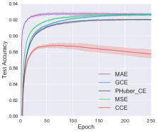
(a) MNIST, linear

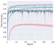
(b) MNIST, MLP

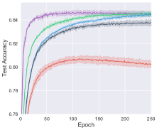
(c) Fashion MNIST, linear

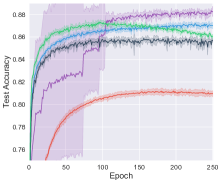
(d) Fashion MNIST, MLP

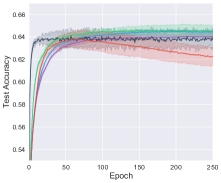
(e) Kuzushiji MNIST, linear

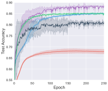
(f) Kuzushiji MNIST, MLP

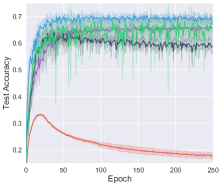
(g) CIFAR-10, ResNet

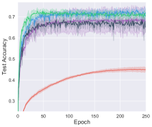
(h) CIFAR-10, DenseNet

Figure 1: Experimental results of different loss functions for different datasets and models. Dark colors show the mean accuracy of 5 trials and light colors show the standard deviation.

• Categorical Cross Entropy (CCE):

  $$\mathcal{L}_{\text{CCE}}(f(\boldsymbol{x}),y)=-\log p_{\boldsymbol{\theta}}(y|\boldsymbol{x}).$$

• Mean Absolute Error (MAE):

  $$\mathcal{L}_{\text{MAE}}(f(\boldsymbol{x}),y)=2-2p_{\boldsymbol{\theta}}(y|\boldsymbol{x}).$$

• Mean Square Error (MSE):

  $$\mathcal{L}_{\text{MSE}}(f(\boldsymbol{x}),y)=1-2p_{\boldsymbol{\theta}}(y|\boldsymbol{x})+\sum\nolimits_{j=1}^{k}p_{\boldsymbol{\theta}}(j|\boldsymbol{x})^{2}.$$

• Generalized Cross Entropy (GCE) (Zhang & Sabuncu, 2018):

  $$\mathcal{L}_{\text{GCE}}(f(\boldsymbol{x}),y)={(1-p_{\boldsymbol{\theta}}(y|\boldsymbol{x})^{q})}/{q},$$

  where $q\in(0,1]$ is a user-defined hyper-parameter. We set $q=0.7$, as suggested by Zhang & Sabuncu (2018).

• Partially Huberised Cross Entropy (PHuber-CE) (Menon et al., 2020):

  $$\small\mathcal{L}_{\text{PHuber-CE}}(f(\boldsymbol{x}),y)=\left\{\begin{matrix}-\log p_{\boldsymbol{\theta}}(y|\boldsymbol{x}),\text{if }p_{\boldsymbol{\theta}}(y|\boldsymbol{x})\geq\frac{1}{\tau},\\ -\tau p_{\boldsymbol{\theta}}(y|\boldsymbol{x})+\log\tau+1,\ \text{else},\end{matrix}\right.$$

  where $\tau>0$ is a user-defined hyper-parameter. We set $\tau=10$, because it works well in Menon et al. (2020).

The detailed derivations of the above loss functions and their bounds are provided in Appendix D. Among these losses, CCE is unbounded while the others are bounded. We will experimentally demonstrate (Figure 1) that by inserting the above losses into Eq. (11), bounded loss is significantly better than unbounded loss. Furthermore, we conduct a deeper analysis of MAE because MAE has the special property that MAE is not only bounded, but also satisfies the symmetric condition (Ghosh et al., 2017), i.e., $\sum_{y=1}^{k}\mathcal{L}_{\text{MAE}}\big{(}f(\boldsymbol{x}),y\big{)}=2k-2$, which means the sum of the losses over all classes is a constant for arbitrary examples. However, is MAE good enough? Previous studies (Zhang & Sabuncu, 2018; Wang et al., 2019) have already shown that MAE suffers from the optimization issue, which would affect its practical performance. To alleviate this problem, we further improve MAE by proposing two upper-bound surrogate loss functions. Specifically, by using MAE in Eq. (11), we obtain

$$\widehat{R}(f)= \frac{k-1}{|\widebar{Y}_{i}|}\sum\nolimits_{y\notin\widebar{Y}_{i}}\mathcal{L}_{\text{MAE}}\big{(}f(\boldsymbol{x}_{i}),y\big{)}$$

$$= \frac{2k-2}{|\widebar{Y}_{i}|}\mathcal{L}^{\prime}_{\text{MAE}}\big{(}f(\boldsymbol{x}_{i}),\widebar{Y}_{i}\big{)}+Z_{i},$$ (12)

where $\mathcal{L}^{\prime}_{\text{MAE}}\big{(}f(\boldsymbol{x}_{i}),\widebar{Y}_{i}\big{)}:=1-\sum_{j\notin\widebar{Y}_{i}}p_{\boldsymbol{\theta}}(j|\boldsymbol{x}_{i})$, and $Z_{i}$ is a constant independent of $f(\boldsymbol{x}_{i})$. It is clear that minimizing $\mathcal{L}^{\prime}_{\text{MAE}}\big{(}f(\boldsymbol{x}_{i}),\widebar{Y}_{i}\big{)}$ is equivalent to minimizing $\sum_{y\notin\widebar{Y}_{i}}\mathcal{L}_{\text{MAE}}\big{(}f(\boldsymbol{x},y)\big{)}$.

Based on this fact, we further introduce two upper-bound surrogate loss functions of $\mathcal{L}^{\prime}_{\text{MAE}}$:

$$\mathcal{L}_{\text{EXP}}(f(\boldsymbol{x}_{i}),\widebar{Y}_{i}) =\exp\Big{(}-\sum\nolimits_{j\notin\widebar{Y}_{i}}p_{\boldsymbol{\theta}}(j|\boldsymbol{x}_{i})\Big{)},$$

$$\mathcal{L}_{\text{LOG}}(f(\boldsymbol{x}_{i}),\widebar{Y}_{i}) =-\log\Big{(}\sum\nolimits_{j\notin\widebar{Y}_{i}}p_{\boldsymbol{\theta}}(j|\boldsymbol{x}_{i})\Big{)}.$$

One can easily verify that $\mathcal{L}_{\text{MAE}}^{\prime}$ is upper bounded by $\mathcal{L}_{\text{EXP}}$ and $\mathcal{L}_{\text{LOG}}$ using the two inequalities $1-z\leq\exp(-z)$ and $1-z\leq-\log z$, respectively. By replacing $\mathcal{L}_{\text{MAE}}^{\prime}$ by $\mathcal{L}_{\text{LOG}}$ and $\mathcal{L}_{\text{LOG}}$ in Eq. (12), we obtain two new methods for learning with MCLs. We explain the advantage of $\mathcal{L}_{\text{EXP}}$ and $\mathcal{L}_{\text{LOG}}$ over $\mathcal{L}_{\text{MAE}}^{\prime}$ by closely examining their gradients:

$$\frac{\partial\mathcal{L}^{\prime}_{\text{MAE}}}{\partial\boldsymbol{\theta}} =\left\{\begin{matrix}-\nabla_{\boldsymbol{\theta}}p_{\boldsymbol{\theta}}(j|\boldsymbol{x}_{i}),&\ \text{if}\ j\notin\widebar{Y}_{i},\\ 0,&\ \text{else},\end{matrix}\right.$$

$$\frac{\partial\mathcal{L}_{\text{EXP}}}{\partial\boldsymbol{\theta}} =\left\{\begin{matrix}-\nabla_{\boldsymbol{\theta}}p_{\boldsymbol{\theta}}(j|\boldsymbol{x}_{i})\cdot w_{\text{EXP}},&\ \text{if}\ j\notin\widebar{Y}_{i},\\ 0,&\ \text{else},\end{matrix}\right.$$

$$\frac{\partial\mathcal{L}_{\text{LOG}}}{\partial\boldsymbol{\theta}} =\left\{\begin{matrix}-\nabla_{\boldsymbol{\theta}}p_{\boldsymbol{\theta}}(j|\boldsymbol{x}_{i})\cdot w_{\text{LOG}},&\ \text{if}\ j\notin\widebar{Y}_{i},\\ 0,&\ \text{else},\end{matrix}\right.$$

where $w_{\text{EXP}}=\exp\big{(}-\sum_{j\notin\widebar{Y}_{i}}p_{\boldsymbol{\theta}}(j|\boldsymbol{x}_{i})\big{)}$ and $w_{\text{LOG}}=\big{(}\sum_{j\notin\widebar{Y}_{i}}p_{\boldsymbol{\theta}}(j|\boldsymbol{x}_{i})\big{)}^{-1}$. From their gradients, we can clearly observe that $\mathcal{L}_{\text{MAE}}^{\prime}$ basically treats each example equally, while $\mathcal{L}_{\text{EXP}}$ and $\mathcal{L}_{\text{LOG}}$ give more weights to difficult examples. Concretely, if $\sum_{j\notin\widebar{Y}_{i}}p_{\boldsymbol{\theta}}(j|\boldsymbol{x}_{i})$ is small, both $w_{\text{EXP}}$ and $w_{\text{LOG}}$ would be large. In other words, $\mathcal{L}_{\text{EXP}}$ and $\mathcal{L}_{\text{LOG}}$ pay more attention to hard examples whose sum of the predicted confidences of all the non-complementary labels is small.

5 Experiments

Table 2: Classification accuracy (mean$\pm$std) of each algorithm on the four UCI datasets using a linear model for 5 trials. The best performance among all the approaches is highlighted in boldface. In addition, $\bullet/\circ$ indicates whether the performance of our approach (the best of EXP and LOG) is statistically superior/inferior to the comparing algorithm on each dataset (paired $t$-test at 0.05 significance level).

Approach		Yeast	Texture	Dermatology	Synthetic Control
Upper-bound Losses	EXP	54.94$\pm$1.56%$\bullet$	97.51$\pm$0.09%$\bullet$	98.89$\pm$0.37%	27.87$\pm$5.13%$\bullet$
	LOG	60.11$\pm$1.93%	98.88$\pm$0.43%	99.46$\pm$1.14%	90.73$\pm$4.41%
Bounded Losses	MAE	33.07$\pm$0.37%$\bullet$	85.29$\pm$7.93%$\bullet$	85.39$\pm$2.58%$\bullet$	23.50$\pm$2.44%$\bullet$
	MSE	58.17$\pm$1.52%$\bullet$	97.59$\pm$0.16%$\bullet$	97.84$\pm$1.21%$\bullet$	34.20$\pm$8.69%$\bullet$
	GCE	57.56$\pm$1.56%$\bullet$	97.25$\pm$0.31%$\bullet$	97.53$\pm$1.81%$\bullet$	23.67$\pm$3.10%$\bullet$
	Phuber-CE	55.54$\pm$1.03%$\bullet$	94.89$\pm$3.28%$\bullet$	95.14$\pm$2.41%$\bullet$	24.71$\pm$3.18%$\bullet$
Unbounded Loss	CCE	49.50$\pm$3.58%$\bullet$	92.08$\pm$1.15%$\bullet$	83.19$\pm$3.65%$\bullet$	63.47$\pm$6.91%$\bullet$
Decomposition before Shuffle	GA	27.91$\pm$5.02%$\bullet$	90.93$\pm$1.34%$\bullet$	36.05$\pm$9.79%$\bullet$	18.12$\pm$1.74%$\bullet$
	NN	32.73$\pm$3.59%$\bullet$	96.29$\pm$0.39%$\bullet$	61.49$\pm$6.83%$\bullet$	55.12$\pm$4.43%$\bullet$
	FREE	35.50$\pm$2.79%$\bullet$	94.36$\pm$1.08%$\bullet$	86.30$\pm$5.62%$\bullet$	76.95$\pm$3.26%$\bullet$
	PC	53.89$\pm$3.53%$\bullet$	92.68$\pm$0.81%$\bullet$	96.27$\pm$3.07%$\bullet$	72.63$\pm$5.86%$\bullet$
	Forward	58.15$\pm$1.54%$\bullet$	98.95$\pm$0.17%	99.37$\pm$0.85%	38.77$\pm$6.06%$\bullet$
Decomposition after Shuffle	GA	28.21$\pm$1.53%$\bullet$	83.66$\pm$2.27%$\bullet$	42.05$\pm$7.94%$\bullet$	25.46$\pm$1.28%$\bullet$
	NN	36.04$\pm$2.24%$\bullet$	93.91$\pm$0.40%$\bullet$	62.54$\pm$9.19%$\bullet$	59.80$\pm$5.14%$\bullet$
	FREE	43.47$\pm$1.36%$\bullet$	93.94$\pm$0.72%$\bullet$	86.22$\pm$6.07%$\bullet$	73.33$\pm$2.17%$\bullet$
	PC	54.58$\pm$2.57%$\bullet$	94.19$\pm$1.21%$\bullet$	95.73$\pm$3.33%$\bullet$	69.53$\pm$9.01%$\bullet$
	Forward	59.46$\pm$1.16%	97.65$\pm$0.32%$\bullet$	99.03$\pm$1.33%	43.57$\pm$5.83%$\bullet$
Partial Label Convex Formulation	CLPL	55.39$\pm$1.21%$\bullet$	92.07$\pm$0.88%$\bullet$	99.42$\pm$0.54%	63.57$\pm$5.46%$\bullet$

Table 3: Classification accuracy (mean$\pm$std) of each algorithm on the four benchmark datasets using a linear model for 5 trials. The best performance among all the approaches is highlighted in boldface. In addition, $\bullet/\circ$ indicates whether the performance of our approach (the best of EXP and LOG) is statistically superior/inferior to the comparing algorithm on each dataset (paired $t$-test at 0.05 significance level).

Approach		MNIST	Kuzushiji	Fashion	20Newsgroups
Upper-bound Losses	EXP	92.67$\pm$0.11%	64.23$\pm$0.33%$\bullet$	84.56$\pm$0.25%	81.72$\pm$0.39%$\bullet$
	LOG	92.58$\pm$0.09%$\bullet$	68.89$\pm$0.25%	84.42$\pm$0.16%	84.06$\pm$0.57%
Bounded Losses	MAE	92.66$\pm$0.12%	64.03$\pm$0.19%$\bullet$	84.50$\pm$0.16%	79.68$\pm$1.40%$\bullet$
	MSE	92.64$\pm$0.13%	64.51$\pm$0.55%$\bullet$	84.53$\pm$0.20%	81.55$\pm$0.52%$\bullet$
	GCE	92.66$\pm$0.12%	64.44$\pm$0.17%$\bullet$	84.44$\pm$0.15%	81.78$\pm$0.60%$\bullet$
	Phuber-CE	92.02$\pm$0.07%$\bullet$	63.81$\pm$0.75%$\bullet$	83.76$\pm$0.22%$\bullet$	73.52$\pm$1.04%$\bullet$
Unbounded Loss	CCE	88.23$\pm$0.19%$\bullet$	62.27$\pm$0.84%$\bullet$	80.25$\pm$0.29%$\bullet$	63.78$\pm$0.79%$\bullet$
Decomposition before Shuffle	GA	85.51$\pm$0.26%$\bullet$	55.61$\pm$0.24%$\bullet$	78.64$\pm$0.33%$\bullet$	76.64$\pm$0.62%$\bullet$
	NN	88.09$\pm$0.16%$\bullet$	60.54$\pm$0.23%$\bullet$	80.68$\pm$0.07%$\bullet$	76.00$\pm$0.37%$\bullet$
	FREE	89.35$\pm$0.14%$\bullet$	65.21$\pm$0.45%$\bullet$	81.22$\pm$0.11%$\bullet$	68.34$\pm$0.72%$\bullet$
	PC	88.21$\pm$0.23%$\bullet$	62.76$\pm$0.40%$\bullet$	80.60$\pm$0.18%$\bullet$	66.91$\pm$1.20%$\bullet$
	Forward	92.57$\pm$0.05%$\bullet$	63.51$\pm$0.22%$\bullet$	84.38$\pm$0.20%	74.69$\pm$1.14%$\bullet$
Decomposition after Shuffle	GA	83.16$\pm$0.22%$\bullet$	56.31$\pm$0.42%$\bullet$	73.37$\pm$0.10%$\bullet$	66.14$\pm$0.79%$\bullet$
	NN	88.79$\pm$0.26%$\bullet$	63.19$\pm$0.12%$\bullet$	79.77$\pm$0.14%$\bullet$	66.35$\pm$0.53%$\bullet$
	FREE	89.02$\pm$0.22%$\bullet$	64.18$\pm$0.18%$\bullet$	80.11$\pm$0.04%$\bullet$	66.16$\pm$0.60%$\bullet$
	PC	87.76$\pm$0.17%$\bullet$	61.64$\pm$0.38%$\bullet$	80.58$\pm$0.17%$\bullet$	65.64$\pm$0.81%$\bullet$
	Forward	92.54$\pm$0.04%$\bullet$	63.69$\pm$0.14%$\bullet$	84.37$\pm$0.17%$\bullet$	71.98$\pm$3.41%$\bullet$
Partial Label Convex Formulation	CLPL	81.85$\pm$0.27%$\bullet$	55.31$\pm$0.23%$\bullet$	77.26$\pm$0.10%$\bullet$	81.48$\pm$0.45%$\bullet$

In this section, we conduct extensive experiments to evaluate the performance of our proposed approaches including the two wrappers, the unbiased risk estimator with various loss functions and the two upper-bound surrogate loss functions.

Table 4: Classification accuracy (mean$\pm$std) of each algorithm on the five benchmark datasets using neural networks for 5 trials. The best performance among all the approaches is highlighted in boldface. In addition, $\bullet/\circ$ indicates whether the performance of our approach (the best of EXP and LOG) is statistically superior/inferior to the comparing algorithm on each dataset (paired $t$-test at 0.05 significance level).

Approach		MNIST	Kuzushiji	Fashion	CIFAR-10 R	CIFAR-10 D	20Newsgroups
Upper-bound Losses	EXP	97.80$\pm$0.06%	88.25$\pm$0.28%	88.07$\pm$0.19%$\bullet$	72.49$\pm$0.84%$\bullet$	75.53$\pm$0.58%	77.22$\pm$1.22%
	LOG	97.86$\pm$0.13%	88.24$\pm$0.08%	88.36$\pm$0.26%	75.38$\pm$0.34%	75.80$\pm$0.62%	79.46$\pm$0.94%
Bounded Losses	MAE	97.81$\pm$0.04%	88.11$\pm$0.40%	88.13$\pm$0.23%	65.57$\pm$4.08%$\bullet$	68.24$\pm$5.84%$\bullet$	49.83$\pm$4.01%$\bullet$
	MSE	96.84$\pm$0.08%$\bullet$	84.97$\pm$0.23%$\bullet$	86.14$\pm$0.04%$\bullet$	63.58$\pm$1.19%$\bullet$	70.89$\pm$0.81%$\bullet$	72.19$\pm$0.59%$\bullet$
	GCE	96.62$\pm$0.08%$\bullet$	85.02$\pm$0.26%$\bullet$	87.03$\pm$0.20%$\bullet$	68.40$\pm$1.05%$\bullet$	71.54$\pm$0.83%$\bullet$	74.96$\pm$0.47%$\bullet$
	Phuber-CE	95.00$\pm$0.36%$\bullet$	80.66$\pm$0.32%$\bullet$	85.52$\pm$0.18%$\bullet$	59.64$\pm$1.21%$\bullet$	66.49$\pm$0.67%$\bullet$	62.63$\pm$2.32%$\bullet$
Unbounded Loss	CCE	88.64$\pm$0.50%$\bullet$	67.86$\pm$1.01%$\bullet$	80.97$\pm$0.23%$\bullet$	18.01$\pm$0.63%$\bullet$	44.94$\pm$1.20%$\bullet$	54.96$\pm$0.38%$\bullet$
Decomposition before Shuffle	GA	96.36$\pm$0.05%$\bullet$	84.35$\pm$0.22%$\bullet$	85.59$\pm$0.30%$\bullet$	69.05$\pm$0.83%$\bullet$	65.38$\pm$1.40%$\bullet$	79.06$\pm$0.57%
	NN	96.70$\pm$0.08%$\bullet$	82.21$\pm$0.36%$\bullet$	86.29$\pm$0.10%$\bullet$	63.85$\pm$0.74%$\bullet$	64.80$\pm$1.28%$\bullet$	76.81$\pm$0.44%$\bullet$
	FREE	88.55$\pm$0.38%$\bullet$	70.32$\pm$0.80%$\bullet$	81.17$\pm$0.36%$\bullet$	32.02$\pm$1.69%$\bullet$	39.22$\pm$0.43%$\bullet$	61.22$\pm$1.24%$\bullet$
	PC	92.74$\pm$0.17%$\bullet$	73.18$\pm$0.59%$\bullet$	83.32$\pm$0.28%$\bullet$	43.16$\pm$2.21%$\bullet$	49.53$\pm$1.18%$\bullet$	65.15$\pm$2.05%$\bullet$
	Forward	97.67$\pm$0.04%$\bullet$	87.65$\pm$0.24%$\bullet$	88.08$\pm$0.24%$\bullet$	71.92$\pm$1.09%$\bullet$	71.30$\pm$1.16%$\bullet$	77.19$\pm$%0.76$\bullet$
Decomposition after Shuffle	GA	92.08$\pm$0.22%$\bullet$	74.64$\pm$0.67%$\bullet$	79.73$\pm$0.19%$\bullet$	53.12$\pm$0.97%$\bullet$	56.51$\pm$0.89%$\bullet$	63.37$\pm$1.16%$\bullet$
	NN	92.47$\pm$0.14%$\bullet$	73.88$\pm$0.63%$\bullet$	82.99$\pm$0.13%$\bullet$	36.79$\pm$0.78%$\bullet$	53.78$\pm$0.92%$\bullet$	65.15$\pm$0.73%$\bullet$
	FREE	88.99$\pm$0.39%$\bullet$	70.09$\pm$0.74%$\bullet$	81.74$\pm$0.23%$\bullet$	15.16$\pm$2.22%$\bullet$	47.45$\pm$0.98%$\bullet$	50.86$\pm$1.56%$\bullet$
	PC	92.94$\pm$0.05%$\bullet$	68.60$\pm$1.32%$\bullet$	82.46$\pm$0.26%$\bullet$	33.16$\pm$0.92%$\bullet$	52.23$\pm$0.88%$\bullet$	64.32$\pm$0.86%$\bullet$
	Forward	97.49$\pm$0.08%$\bullet$	86.47$\pm$0.39%$\bullet$	87.56$\pm$0.14%$\bullet$	72.16$\pm$0.97%$\bullet$	75.23$\pm$1.02%	79.35$\pm$0.82%

Datasets.  We use five widely-used benchmark datasets MNIST (LeCun et al., 1998), Kuzushiji-MNIST (Clanuwat et al., 2018), Fashion-MNIST (Xiao et al., 2017), 20Newsgroups (Lang, 1995), and CIFAR-10 (Krizhevsky et al., 2009), and four datasets from the UCI repository (Blake & Merz, 1998). We use four base models including linear model, MLP model ($d$-500-$k$), ResNet (34 layers) (He et al., 2016), and DenseNet (22 layers) (Huang et al., 2017). The detailed descriptions of these datasets with the corresponding base models are provided in Appendix E.1. To generate MCLs, we instantiate $p(s)=\tbinom{k-1}{s}/(2^{k}-2)$, $\forall s\in\{1,\cdots,k-1\}$, which means $p(s)$ represents the ratio of the number of label sets whose size is $s$ to the number of all possible label sets. For each instance $\boldsymbol{x}$, we first randomly sample $s$ from $p(s)$, and then uniformly and randomly sample a complementary label set $\widebar{Y}$ with size $s$ (i.e., $p(\widebar{Y})=1/\tbinom{k-1}{s}$).

Approaches.  We absorb five ordinary complementary-label learning approaches in the two wrappers (introduced in Section 4.1): GA, NN, and Free (Ishida et al., 2019), PC (Ishida et al., 2017), and Forward (Yu et al., 2018).We also use an unbounded loss CCE and four bounded losses MAE, MSE, GCE (Zhang & Sabuncu, 2018), and PHuber-CE (Menon et al., 2020) in our empirical estimator Eq. (11). Besides, two upper-bound loss functions LOG and EXP are also inserted into Eq. (12). In addition, we also compare with a representative partial label learning approach CLPL (Cour et al., 2011). For all the approaches, we adopt the same base model for fair comparison. Learning rate and weight decay are selected from $\{10^{-6},10^{-5},\cdots,10^{-1}\}$. We implement our approach using PyTorch, and use the Adam (Kingma & Ba, 2015) optimization method with mini-batch size set to 256 and epoch number set to 250. Hyper-parameters for all the approaches are selected so as to maximize the accuracy on a validation set (10% of the training set) of complementarily labeled data. All the experiments are conducted on NVIDIA Tesla V100 GPUs.

Loss Comparison.  Figure 1 shows the mean and standard deviation of test accuracy of 5 trials, for bounded loss functions MAE, MSE, GCE, PHuber-CE, and unbounded loss function CCE used in our empirical risk estimator Eq. (11). We also record the mean and standard deviation of training accuracy (the training set is evaluated with ordinary labels) of 5 trials, and put the results in Appendix E.2. As can be seen from Figure 1, all the bounded losses are significantly better than the unbounded loss CCE in our formulation. This observation clearly accords with our discussion on the over-fitting issue in Section 4.3. In addition, MAE achieves comparable performance compared with other bounded losses in most cases, while it is sometimes inferior to other bounded losses due to its optimization issue (Zhang & Sabuncu, 2018). Both the advantage and disadvantage of MAE motivate us to use the upper-bound loss functions EXP and LOG for improving the classification performance.

Performance Comparison.  Table 2, Table 3, and Table 4 show the experimental results of different approaches using a linear model or neural networks on the four UCI datasets and the other five benchmark datasets. In table 4, “CIFAR-10 R” and “CIFAR-10 D” mean that we use ResNet and DenseNet on CIFAR-10. Note that CLPL is a convex approach for partial label learning, which is specially designed with a linear model. Hence CLPL does not appear in Table 4. From the three tables, we can find that equipped with the two wrappers “Decomposition before Shuffle” and “Decomposition after Shuffle”, ordinary complementary-label learning approaches work well for learning with MCLs. However, they are significantly outperformed by the upper-bound losses in most cases, which also achieve the best performance among all the approaches on various benchmark datasets. In addition, we also study the case where the size of each complementary label set $s$ is fixed at $j$ (i.e., $p(s=j)=1$) while increasing $j$ from 1 to $k-2$. The corresponding experimental results are provided in Appendix E.3, which show that the classification accuracy of our approaches increases as $j$ increases. This observation is clearly in accordance with our derived estimation error bound (Theorem 4), as the estimation error would decrease if $j$ increases.

6 Conclusion

In this paper, we propose a novel problem setting called learning with multiple complementary labels (MCLs), which is a generation of complementary-label learning (Ishida et al., 2017; Yu et al., 2018; Ishida et al., 2019). To solve this learning problem, we first design two wrappers that enable us to use arbitrary complementary-label learning approaches for learning with MCLs. However, we find that the supervision information that MCLs hold is conceptually diluted after decomposition. Therefore, we further propose an unbiased risk estimator for learning with MCLs, which processes each set of MCLs as a whole. Then, we theoretically derive an estimation error bound, which guarantees the learning consistency. Although our risk estimator does not rely on specific models or loss functions, we show that bounded loss is generally better than unbounded loss in our empirical risk estimator. In addition, we improve the risk estimator into minimizing properly chosen upper bounds for practical implementation. Extensive experiments demonstrate the effectiveness of the proposed approaches.

Appendix A Proofs about the Problem Setting

A.1 Proofs of Theorem 1

Firstly, we define the set of all the possible label sets whose size is $j$ as

$$\widebar{\mathcal{Y}}_{j}:=\{Y\mid Y\in\widebar{\mathcal{Y}},|Y|=j\}.$$

Then, by the definition of $\widebar{p}(\boldsymbol{x},\widebar{Y})$, we can obtain

$$\int_{\widebar{\mathcal{Y}}}\int_{\mathcal{X}}{\widebar{p}(\boldsymbol{x},\widebar{Y})}\mathrm{d}\boldsymbol{x}\ \mathrm{d}\widebar{Y} =\int\sum\nolimits_{\widebar{Y}\in\widebar{\mathcal{Y}}}\widebar{p}(\boldsymbol{x},\widebar{Y})\text{d}\boldsymbol{x}$$

$$=\int\sum\nolimits_{\widebar{Y}\in\widebar{\mathcal{Y}}}\sum\nolimits_{j=1}^{k-1}\Big{(}\widebar{p}(\boldsymbol{x},\widebar{Y}\mid s=j)p(s=j)\Big{)}\text{d}\boldsymbol{x}$$

$$=\int\sum\nolimits_{j=1}^{k-1}\sum\nolimits_{\widebar{Y}\in\widebar{\mathcal{Y}}_{j}}\Big{(}\widebar{p}(\boldsymbol{x},\widebar{Y}\mid s=j)p(s=j)\Big{)}\text{d}\boldsymbol{x}\quad\quad(\because\widebar{\mathcal{Y}}_{j}:=\{\widebar{Y}\mid\widebar{Y}\in\mathcal{\widebar{Y}},|\widebar{Y}|=j\})$$

$$=\int\sum\nolimits_{j=1}^{k-1}\sum\nolimits_{\widebar{Y}\in\widebar{\mathcal{Y}}_{j}}\bigg{(}\frac{1}{\tbinom{k-1}{j}}\sum\nolimits_{y\notin\widebar{Y}}p(\boldsymbol{x},y)p(s=j)\bigg{)}\text{d}\boldsymbol{x}\quad\quad(\because\text{the definition of }\widebar{p}(\boldsymbol{x},\widebar{Y}\mid s=j))$$

$$=\int\sum\nolimits_{j=1}^{k-1}\bigg{(}\frac{1}{\tbinom{k-1}{j}}\frac{\tbinom{k}{j}(k-j)}{k}\sum\nolimits_{y=1}^{k}p(\boldsymbol{x},y)p(s=j)\bigg{)}\text{d}\boldsymbol{x}\quad\quad\big{(}\because|\widebar{\mathcal{Y}}_{j}|=\tbinom{k}{j}\big{)}$$

$$=\int\sum\nolimits_{j=1}^{k-1}p(\boldsymbol{x})p(s=j)\text{d}\boldsymbol{x}$$

$$=1,$$

which concludes the proof of Theorem 1.∎

A.2 Proof of Lemma 1

Let us consider the case where the correct label $y$ is a specific label $i$ $(i\in\{1,2,\cdots,k\})$, then we have

$$p(y\in\widebar{Y},y=i\mid\boldsymbol{x},s)= p(y\in\widebar{Y}\mid y=i,\boldsymbol{x},s)p(y=i\mid\boldsymbol{x},s)$$

$$= \sum\nolimits_{C\in\widebar{\mathcal{Y}}}p(y\in\widebar{Y},\widebar{Y}=C\mid y=i,\boldsymbol{x},s)p(y=i\mid\boldsymbol{x},s).$$

Here, $p(y=i\mid\boldsymbol{x},s)=p(y=i\mid\boldsymbol{x})$ since the labeling rule is independent of $s$. In addition, $\sum\nolimits_{C\in\widebar{\mathcal{Y}}}p(y\in\widebar{Y},\widebar{Y}=C\mid y=i,\boldsymbol{x},s)=\sum\nolimits_{C\in\widebar{\mathcal{Y}}_{s}}p(y\in\widebar{Y},\widebar{Y}=C\mid y=i,\boldsymbol{x})$ since given the size $s$ of the label set, the whole set of all the possible label sets becomes $\widebar{\mathcal{Y}}_{s}$. Then, we can obtain

$$p(y\in\widebar{Y},y=i\mid\boldsymbol{x},s)= \sum\nolimits_{C\in\widebar{\mathcal{Y}}}p(y\in\widebar{Y},\widebar{Y}=C\mid y=i,\boldsymbol{x},s)p(y=i\mid\boldsymbol{x},s)$$

$$= \sum\nolimits_{C\in\widebar{\mathcal{Y}}_{s}}p(y\in\widebar{Y},\widebar{Y}=C\mid y=i,\boldsymbol{x})p(y=i\mid\boldsymbol{x})$$

$$= \sum\nolimits_{C\in\widebar{\mathcal{Y}}_{s}}p(y\in\widebar{Y}\mid\widebar{Y}=C,y=i,\boldsymbol{x})p(y=i\mid\boldsymbol{x})p(\widebar{Y}=C\mid\boldsymbol{x})$$

$$= \sum\nolimits_{C\in\widebar{\mathcal{Y}}_{s}}p(y\in\widebar{Y}|\widebar{Y}=C,y=i,\boldsymbol{x})p(y=i|\boldsymbol{x})p(\widebar{Y}=C),$$

where the last equality holds due to the fact that for each instance $\boldsymbol{x}$, $\widebar{Y}$ is uniformly and randomly chosen. Since $p(\widebar{Y}=C)=\frac{1}{|{\widebar{\mathcal{Y}}}_{s}|}$ if $C\in\widebar{\mathcal{Y}}_{s}$ where $|\widebar{\mathcal{Y}}_{s}|=\tbinom{k}{s}$, we have

$$p(y\in\widebar{Y},y=i\mid\boldsymbol{x},s)= \sum\nolimits_{C\in\widebar{\mathcal{Y}}_{s}}p(y\in\widebar{Y}|\widebar{Y}=C,y=i,\boldsymbol{x})p(y=i|\boldsymbol{x})p(\widebar{Y}=C)$$

$$= \frac{1}{\tbinom{k}{s}}\sum\nolimits_{C\in\widebar{\mathcal{Y}}_{s}}p(y\in\widebar{Y}|\widebar{Y}=C,y=i,\boldsymbol{x})p(y=i|\boldsymbol{x})$$

$$= \frac{1}{\tbinom{k}{s}}|\widebar{\mathcal{Y}}_{s}^{i}|p(y=i|\boldsymbol{x})\quad\quad\big{(}\because\widebar{\mathcal{Y}}_{s}^{i}:=\{\widebar{Y}\in\widebar{\mathcal{Y}}_{s}\ |\ i\in\widebar{Y}\}\big{)}$$

$$= \frac{\tbinom{k-1}{s-1}}{\tbinom{k}{s}}p(y=i|\boldsymbol{x})\quad\quad\Big{(}\because|\widebar{\mathcal{Y}}_{s}^{i}|=\tbinom{k-1}{s-1}\Big{)}$$

$$= \frac{s}{k}p(y=i|\boldsymbol{x}).$$

By further summing up the both side over all the possible $i$, we can obtain

$$p(y\in\widebar{Y}|\boldsymbol{x},s)=\frac{s}{k},$$

which concludes the proof of Lemma 1.∎

A.3 Proof of Theorem 2

Let us express $p(\widebar{Y}|y\notin\widebar{Y},\boldsymbol{x},s)$ as

$$p(\widebar{Y}|y\notin\widebar{Y},\boldsymbol{x},s)= \frac{p(y\notin\widebar{Y},\widebar{Y}|\boldsymbol{x},s)}{p(y\notin\widebar{Y}|\boldsymbol{x},s)}$$

$$= \frac{p(y\notin\widebar{Y}|\widebar{Y},\boldsymbol{x},s)p(\widebar{Y}|\boldsymbol{x},s)}{p(y\notin\widebar{Y}|\boldsymbol{x},s)}$$

$$= \frac{p(y\notin\widebar{Y}|\widebar{Y},\boldsymbol{x},s)p(\widebar{Y}|s)}{p(y\notin\widebar{Y}|\boldsymbol{x},s)},$$

where the last equality holds because $\widebar{Y}$ is influenced by the size $s$, and for each instance $\boldsymbol{x}$, $\widebar{Y}$ is uniformly and randomly chosen. Note that given $s$, there are $|\widebar{\mathcal{Y}}_{s}|$ possible label sets, thus $p(\widebar{Y}|s)=\frac{1}{|\widebar{\mathcal{Y}}_{s}|}$ where $|\widebar{\mathcal{Y}}_{s}|=\tbinom{k}{s}$. In this way, we have

$$p(\widebar{Y}|y\notin\widebar{Y},\boldsymbol{x},s)= \frac{p(y\notin\widebar{Y}|\widebar{Y},\boldsymbol{x},s)p(\widebar{Y}|s)}{p(y\notin\widebar{Y}|\boldsymbol{x},s)}$$

$$= \frac{1}{\tbinom{k}{s}}\frac{p(y\notin\widebar{Y}|\widebar{Y},\boldsymbol{x},s)}{1-p(y\in\widebar{Y}|\boldsymbol{x},s)}$$

$$= \frac{1}{\tbinom{k}{s}}\frac{1}{1-\frac{s}{k}}p(y\notin\widebar{Y}|\widebar{Y},\boldsymbol{x},s)\quad\quad\Big{(}\because\text{by Lemma 1, }p(y\in\widebar{Y}|\boldsymbol{x},s)=\frac{s}{k}\Big{)}$$

$$= \frac{1}{\tbinom{k}{s}}\frac{k}{k-s}\sum\nolimits_{y\notin\widebar{Y}}p(y|\boldsymbol{x},s)$$

$$= \frac{1}{\tbinom{k-1}{s}}\sum\nolimits_{y\notin\widebar{Y}}p(y|\boldsymbol{x}).$$

By multiplying $p(\boldsymbol{x})$ on both side, we have

$$p(\boldsymbol{x},\widebar{Y}|y\notin\widebar{Y},s)=\frac{1}{\tbinom{k-1}{s}}\sum\nolimits_{y\notin\widebar{Y}}p(\boldsymbol{x},y).$$

Then taking into account the variable $s$, we have

$$p(\boldsymbol{x},\widebar{Y}|y\notin\widebar{Y})= \sum\nolimits_{j=1}^{k-1}p(s=j)p(\boldsymbol{x},\widebar{Y}|y\notin\widebar{Y},s=j)$$

$$= \sum\nolimits_{j=1}^{k-1}p(s=j)\frac{1}{\tbinom{k-1}{j}}\sum\nolimits_{y\notin\widebar{Y}}p(\boldsymbol{x},y)$$

$$= \widebar{p}(\boldsymbol{x},\widebar{Y}),$$

which concludes the proof.∎

Appendix B Proofs of the Unbiased Risk Estimator

B.1 Proof of Lemma 2

According to our defined distribution, we have already obtained

$$\widebar{p}(\boldsymbol{x},\widebar{Y}\mid s=j)=\frac{1}{\tbinom{k-1}{j}}\sum\nolimits_{y^{\prime}\notin\widebar{Y}}p(\boldsymbol{x},y^{\prime}).$$

Then, we can obtain the following equality by operating $\sum\nolimits_{\widebar{Y}\in\widebar{\mathcal{Y}}_{j}^{y}}$ on both the left and the right hand side:

$$\sum\nolimits_{\widebar{Y}\in\widebar{\mathcal{Y}}_{j}^{y}}\widebar{p}(\widebar{Y}\mid\boldsymbol{x},s=j)=\frac{1}{\tbinom{k-1}{j}}\sum\nolimits_{\widebar{Y}\in\widebar{\mathcal{Y}}_{j}^{y}}\sum\nolimits_{y^{\prime}\notin\widebar{Y}}p(y^{\prime}\mid\boldsymbol{x}),$$ (13)

where $\widebar{\mathcal{Y}}_{j}^{y}:=\{\widebar{Y}\in\widebar{\mathcal{Y}}\mid y\in\widebar{Y},|\widebar{Y}|=j\}$. In this way, the right hand side of the above equality can be transformed by the following derivations:

$$\frac{1}{\tbinom{k-1}{j}}\sum\nolimits_{\widebar{Y}\in\widebar{\mathcal{Y}}_{j}^{y}}\sum\nolimits_{y^{\prime}\notin\widebar{Y}}p(y^{\prime}\mid\boldsymbol{x})= \frac{1}{\tbinom{k-1}{j}}\sum\nolimits_{\widebar{Y}\in\widebar{\mathcal{Y}}_{j}^{y}}\bigg{(}1-\sum\nolimits_{y^{\prime}\in\widebar{Y}}p(y^{\prime}\mid\boldsymbol{x})\bigg{)}$$

$$= \frac{|\widebar{\mathcal{Y}}_{j}^{y}|}{\tbinom{k-1}{j}}-\frac{1}{\tbinom{k-1}{j}}\sum\nolimits_{\widebar{Y}\in\widebar{\mathcal{Y}}_{j}^{y}}\sum\nolimits_{y^{\prime}\in\widebar{Y}}p(y^{\prime}\mid\boldsymbol{x})$$

$$= \frac{\tbinom{k-1}{j-1}}{\tbinom{k-1}{j}}-\frac{1}{\tbinom{k-1}{j}}\sum\nolimits_{y^{\prime}}\sum\nolimits_{\widebar{Y}^{\prime}\in\{\widebar{Y}^{\prime}\in\widebar{\mathcal{Y}}_{j}^{y}|y^{\prime}\in\widebar{Y}^{\prime}\}}p(y^{\prime}\mid\boldsymbol{x})\quad\quad\big{(}\because|\widebar{\mathcal{Y}}_{j}^{y}|=\tbinom{k-1}{j-1}\big{)}$$

$$= \frac{j}{k-j}-\frac{1}{\tbinom{k-1}{j}}\left\{\tbinom{k-1}{j-1}p(y\mid\boldsymbol{x})+\tbinom{k-2}{j-2}\sum\nolimits_{y^{\prime}\neq y}p(y^{\prime}\mid\boldsymbol{x})\right\}$$

$$= \frac{j}{k-j}-\frac{1}{\tbinom{k-1}{j}}\left\{\tbinom{k-1}{j-1}p(y\mid\boldsymbol{x})+\tbinom{k-2}{j-2}\big{(}1-p(y\mid\boldsymbol{x})\big{)}\right\}$$

$$= \frac{j}{k-j}-\frac{1}{\tbinom{k-1}{j}}\left\{\tbinom{k-2}{j-2}+\tbinom{k-2}{j-1}p(y\mid\boldsymbol{x})\right\}\quad\quad\big{(}\because\tbinom{k-2}{j-1}=\tbinom{k-1}{j-1}-\tbinom{k-2}{j-2}\big{)}$$

$$= \frac{j}{k-j}-\frac{j(j-1)}{(k-j)(k-1)}-\frac{j}{k-1}p(y\mid\boldsymbol{x})$$

$$= \frac{j}{k-1}-\frac{j}{k-1}p(y\mid\boldsymbol{x}).$$ (14)

Combing Eq. (13) and Eq. (14), we obtain

$$p(y\mid\boldsymbol{x},s=j)=p(y\mid\boldsymbol{x})=1-\frac{k-1}{j}\sum\nolimits_{\widebar{Y}\in\widebar{\mathcal{Y}}_{j}^{y}}\widebar{p}(\widebar{Y}\mid\boldsymbol{x},s=j).$$ (15)

In the end, by taking into account the variable $s$, we have

$$p(y\mid\boldsymbol{x}) =\sum\nolimits_{j=1}^{k-1}p(s=j)p(y\mid\boldsymbol{x},s=j)$$

$$=\sum\nolimits_{j=1}^{k-1}p(s=j)\Big{(}1-\frac{k-1}{j}\sum\nolimits_{\widebar{Y}\in\widebar{\mathcal{Y}}_{j}^{y}}\widebar{p}(\widebar{Y}\mid\boldsymbol{x},s=j)\Big{)}$$

$$=1-\sum\nolimits_{j=1}^{k-1}\Big{(}\frac{k-1}{j}\sum\nolimits_{\widebar{Y}\in\widebar{\mathcal{Y}}_{j}^{y}}\widebar{p}(\widebar{Y},s=j\mid\boldsymbol{x})\Big{)},$$

which concludes the proof of Lemma 2.

B.2 Proof of Theorem 3

It is intuitive to obtain

$$R(f)=\mathbb{E}_{p(\boldsymbol{x},y)}\big{[}\mathcal{L}\big{(}f(\boldsymbol{x}),y\big{)}\big{]}=\sum\nolimits_{j=1}^{k-1}p(s=j)\mathbb{E}_{p(\boldsymbol{x},y\mid s=j)}\big{[}\mathcal{L}\big{(}f(\boldsymbol{x}),y\big{)}\big{]}.$$

Then, we express the right hand side for each $j\in\{1,\ldots,k-1\}$ as

$$\mathbb{E}_{p(\boldsymbol{x},y\mid s=j)}\big{[}\mathcal{L}\big{(}f(\boldsymbol{x}),y\big{)}\big{]} =\mathbb{E}_{p(\boldsymbol{x}\mid s=j)}\mathbb{E}_{p(y|\boldsymbol{x},s=j)}\big{[}\mathcal{L}\big{(}f(\boldsymbol{x}),y\big{)}\big{]}$$

$$=\mathbb{E}_{p(\boldsymbol{x}\mid s=j)}\bigg{[}\sum\nolimits_{y=1}^{k}p(y|\boldsymbol{x},s=j)\mathcal{L}\big{(}f(\boldsymbol{x}),y\big{)}\bigg{]}\quad\quad$$

$$=\mathbb{E}_{p(\boldsymbol{x}\mid s=j)}\bigg{[}\sum\nolimits_{y=1}^{k}\bigg{(}1-\frac{k-1}{j}\sum\nolimits_{\widebar{Y}\in\widebar{\mathcal{Y}}_{j}^{y}}\widebar{p}(\widebar{Y}|\boldsymbol{x},s=j)\bigg{)}\mathcal{L}\big{(}f(\boldsymbol{x}),y\big{)}\bigg{]}\quad\quad(\because\text{Eq. }(\ref{proof_b1}))$$

$$=\mathbb{E}_{p(\boldsymbol{x}\mid s=j)}\bigg{[}\sum\nolimits_{y=1}^{k}\mathcal{L}\big{(}f(\boldsymbol{x}),y\big{)}-\frac{k-1}{j}\sum\nolimits_{y=1}^{k}\sum\nolimits_{\widebar{Y}\in\widebar{\mathcal{Y}}_{j}^{y}}\widebar{p}(\widebar{Y}|\boldsymbol{x},s=j)\mathcal{L}\big{(}f(\boldsymbol{x}),y\big{)}\bigg{]}$$

$$=\mathbb{E}_{p(\boldsymbol{x}\mid s=j)}\bigg{[}\sum\nolimits_{y=1}^{k}\mathcal{L}\big{(}f(\boldsymbol{x}),y\big{)}-\frac{k-1}{j}\sum\nolimits_{\widebar{Y}\in\widebar{\mathcal{Y}}_{j}}\sum\nolimits_{y^{\prime}\in\widebar{Y}}\widebar{p}(\widebar{Y}|\boldsymbol{x},s=j)\mathcal{L}\big{(}f(\boldsymbol{x}),y\big{)}\bigg{]}$$

$$=\mathbb{E}_{p(\boldsymbol{x}\mid s=j)}\bigg{[}\sum\nolimits_{y=1}^{k}\mathcal{L}\big{(}f(\boldsymbol{x}),y\big{)}-\frac{k-1}{j}\sum\nolimits_{\widebar{Y}\in\widebar{\mathcal{Y}}_{j}}\widebar{p}(\widebar{Y}|\boldsymbol{x},s=j)\Big{(}\sum\nolimits_{y^{\prime}\in\widebar{Y}}\mathcal{L}\big{(}f(\boldsymbol{x}),y^{\prime}\big{)}\Big{)}\bigg{]}$$

$$=\mathbb{E}_{p(\boldsymbol{x}\mid s=j)}\mathbb{E}_{\widebar{p}(\widebar{Y}|\boldsymbol{x},s=j)}\bigg{[}\sum\nolimits_{y=1}^{k}\mathcal{L}\big{(}f(\boldsymbol{x}),y\big{)}-\frac{k-1}{j}\sum\nolimits_{y^{\prime}\in\widebar{Y}}\mathcal{L}\big{(}f(\boldsymbol{x}),y^{\prime}\big{)}\bigg{]}$$

$$=\mathbb{E}_{\widebar{p}(\boldsymbol{x},\widebar{Y}\mid s=j)}\bigg{[}\sum\nolimits_{y\notin\widebar{Y}}\mathcal{L}\big{(}f(\boldsymbol{x}),y^{\prime}\big{)}-\frac{k-1-j}{j}\sum\nolimits_{y^{\prime}\in\widebar{Y}}\mathcal{L}\big{(}f(\boldsymbol{x}),y^{\prime}\big{)}\bigg{]}$$

$$=\mathbb{E}_{\widebar{p}(\boldsymbol{x},\widebar{Y}\mid s=j)}[\widebar{\mathcal{L}}_{j}\big{(}f(\boldsymbol{x}),\widebar{Y}\big{)}]$$

$$=\widebar{R}_{j}(f).$$

In this way, we can obtain $R(f)=\sum\nolimits_{j=1}^{k-1}p(s=j)\widebar{R}_{j}(f)$, which concludes the proof of Theorem 3.∎

Appendix C Proof of Theorem 4

Recall that the expected risk and empirical risk are represented as

$$R(f) =\sum\nolimits_{j=1}^{k-1}p(s=j)\widebar{R}_{j}(f)=\sum\nolimits_{j=1}^{k-1}p(s=j)\mathbb{E}_{p(\boldsymbol{x},\widebar{Y}\mid s=j)}[\widebar{\mathcal{L}}_{j}\big{(}f(\boldsymbol{x}),\widebar{Y}\big{)}],$$

$$\widehat{R}(f) =\sum\nolimits_{j=1}^{k-1}\frac{p(s=j)}{n_{j}}\sum\nolimits_{i=1}^{n_{j}}\widebar{\mathcal{L}}_{j}\big{(}f(\boldsymbol{x}_{i}),\widebar{Y}_{i}\big{)}.$$

Here, with a slight abuse of notation, we simply write $\widebar{R}_{j}(f)$ as $R_{j}(f)$, and define $\widehat{R}_{j}(f)=1/{n_{j}}\sum\nolimits_{i=1}^{n_{j}}\widebar{\mathcal{L}}_{j}\big{(}f(\boldsymbol{x}_{i}),\widebar{Y}_{i}\big{)}$. Thus we have $R(f)=\sum_{j=1}^{k-1}p(s=j){R}_{j}(f)$ and $\widehat{R}(f)=\sum_{j=1}^{k-1}p(s=j)\widehat{R}_{j}(f)$. Since $f^{\star}=\arg\min\nolimits_{f\in\mathcal{F}}R(f)$ and $\widehat{f}=\arg\min\nolimits_{f\in\mathcal{F}}\widehat{R}(f)$, we can obtain the following lemma.

Lemma 3.

The following inequality holds:

$$R(\widehat{f})-R(f^{\star})\leq 2\sum\nolimits_{j=1}^{k-1}p(s=j)\sup_{f\in\mathcal{F}}\left|\widehat{R}_{j}(f)-R_{j}(f)\right|.$$

Proof.

It would be intuitive to obtain

$$R(\widehat{f})-R(f^{\star})= R(\widehat{f})-\widehat{R}(\widehat{f})+\widehat{R}(\widehat{f})-R(f^{\star})$$

$$\leq R(\widehat{f})-\widehat{R}(\widehat{f})+R(\widehat{f})-R(f^{\star})$$

$$\leq 2\sup_{f\in\mathcal{F}}\left|\widehat{R}(f)-R(f)\right|$$

$$= 2\sup_{f\in\mathcal{F}}\left|\sum\nolimits_{j=1}^{k-1}p(s=j)\widehat{R}_{j}(f)-\sum\nolimits_{j=1}^{k-1}p(s=j)R_{j}(f)\right|$$

$$\leq 2\sum\nolimits_{j=1}^{k-1}p(s=j)\sup_{f\in\mathcal{F}}\left|\widehat{R}_{j}(f)-R_{j}(f)\right|,$$

which concludes the proof of Lemma 3. ∎

In this way, we will bound $\sup\nolimits_{f\in\mathcal{F}}\left|\widehat{R}_{j}(f)-R_{j}(f)\right|$ for $j=\{1,\ldots,k-1\}$. Before that, we define a function space as

$$\mathcal{H}_{j}:=\{(\boldsymbol{x},\widebar{Y})\in\mathcal{X}\times\widebar{\mathcal{Y}}_{j}\mapsto\widebar{\mathcal{L}}_{j}\big{(}f(\boldsymbol{x}),\widebar{Y}\big{)}\ |\ f\in\mathcal{F}\},$$

where

$$\widebar{\mathcal{L}}_{j}\big{(}f(\boldsymbol{x}),\widebar{Y}\big{)}:=\sum\nolimits_{y\notin\widebar{Y}}\mathcal{L}\big{(}f(\boldsymbol{x}),y\big{)}-\frac{k-1-j}{j}\sum\nolimits_{y^{\prime}\in\widebar{Y}}\mathcal{L}\big{(}f(\boldsymbol{x}),y^{\prime}\big{)}.$$

Besides, we introduce the definition of Rademacher complexity (Bartlett & Mendelson, 2002).

Definition 1 (Rademacher complexity (Bartlett & Mendelson, 2002)).

Let $Z_{1},\dots,Z_{n}$ be $n$ i.i.d. random variables drawn from a probability distribution $\mathcal{D}$, $\mathcal{H}=\{h:\mathcal{Z}\rightarrow\mathbb{R}\}$ be a class of measurable functions. Then the expected Rademacher complexity of $\mathcal{H}$ is defined as

$$\mathfrak{R}_{n}(\mathcal{H})=\mathbb{E}_{Z_{1},\dots,Z_{n}\sim\mathcal{D}}\mathbb{E}_{\boldsymbol{\sigma}}\bigg{[}\sup\nolimits_{h\in\mathcal{H}}\frac{1}{n}\sum\nolimits_{i=1}^{n}\sigma_{i}h(Z_{i})\bigg{]},$$

where $\boldsymbol{\sigma}=(\sigma_{1},\dots,\sigma_{n})$ are Rademacher variables taking the value from $\{-1,+1\}$ with even probabilities.

Then, we have the following lemma.

Lemma 4.

Let $C_{\mathcal{L}}=\sup\nolimits_{\boldsymbol{x}\in\mathcal{X},f\in\mathcal{F},y\in\mathcal{Y}}\mathcal{L}\big{(}f(\boldsymbol{x}),y\big{)}$. Then, for all $j=\{1,\ldots,k-1\}$, for any $\delta>0$, with probability at least $1-\delta$,

$$\sup_{f\in\mathcal{F}}\left|\widehat{R}_{j}(f)-R_{j}(f)\right|\leq 2\widebar{\mathfrak{R}}_{n_{j}}(\mathcal{H}_{j})+(2k-2j-1)C_{\mathcal{L}}\sqrt{\frac{\log\frac{2}{\delta}}{2n_{j}}},$$ (16)

where

$$\widebar{\mathfrak{R}}_{n_{j}}(\mathcal{H}_{j})=\mathbb{E}_{(\boldsymbol{x}_{i},\widebar{Y}_{i})\sim\widebar{p}(\boldsymbol{x},\widebar{Y}\mid s=j)}\mathbb{E}_{\boldsymbol{\sigma}}\bigg{[}\sup_{h\in\mathcal{H}_{j}}\frac{1}{n_{j}}\sum\nolimits_{i=1}^{n_{j}}\sigma_{i}h(\boldsymbol{x}_{i},\widebar{Y}_{i})\bigg{]}.$$ (17)

Proof.

To prove this lemma, we first show that the single direction $\sup_{f\in\mathcal{F}}\big{(}\widehat{R}_{j}(f)-R_{j}(f)\big{)}$ is bounded with probability at least $1-\frac{\delta}{2}$, and the other direction can be similarly proved. By the definition of $\widebar{\mathcal{L}}_{j}$, we can easily know the possible maximum of $\widebar{\mathcal{L}}_{j}$ is $(k-j)C_{\mathcal{L}}$, and the possible minimum is $-(k-1-j)C_{\mathcal{L}}$. Suppose an example $(\boldsymbol{x}_{i},\widebar{Y}_{i})$ is replaced by another arbitrary example $(\boldsymbol{x}_{i}^{\prime},\widebar{Y}_{i}^{\prime})$, then the change of $\sup_{f\in\mathcal{F}}\big{(}\widehat{R}_{j}(f)-R_{j}(f)\big{)}$ is no greater than $((2k-2j-1)C_{\mathcal{L}})/n_{j}$. Then, by applying McDiarmid’s inequality (McDiarmid, 1989), for any $\delta>0$, with probability at least $1-\frac{\delta}{2}$,

$$\sup_{f\in\mathcal{F}}\big{(}\widehat{R}_{j}(f)-R_{j}(f)\big{)}\leq\mathbb{E}\Big{[}\sup_{f\in\mathcal{F}}\big{(}\widehat{R}_{j}(f)-R_{j}(f)\big{)}\Big{]}+(2k-2j-1)C_{\mathcal{L}}\sqrt{\frac{\log\frac{2}{\delta}}{2n_{j}}}.$$ (18)

In addition, it is routine (Mohri et al., 2012) to show

$$\mathbb{E}\Big{[}\sup_{f\in\mathcal{F}}\big{(}\widehat{R}_{j}(f)-R_{j}(f)\big{)}\Big{]}\leq 2\widebar{\mathfrak{R}}_{n_{j}}(\mathcal{H}_{j}),$$ (19)

Combing Eq. (18) and Eq. (19), we have for any $\delta>0$, with probability at least $1-\frac{\delta}{2}$,

$$\sup_{f\in\mathcal{F}}\big{(}\widehat{R}_{j}(f)-R_{j}(f)\big{)}\leq 2\widebar{\mathfrak{R}}_{n_{j}}(\mathcal{H}_{j})+(2k-2j-1)C_{\mathcal{L}}\sqrt{\frac{\log\frac{2}{\delta}}{2n_{j}}}.$$ (20)

By further taking into account the other side $\sup_{f\in\mathcal{F}}\big{(}R_{j}(f)-\widehat{R}_{j}(f)\big{)}$, we have for any $\delta>0$, with probability at least $1-\delta$,

$$\sup_{f\in\mathcal{F}}\left|\widehat{R}_{j}(f)-R_{j}(f)\right|\leq 2\widebar{\mathfrak{R}}_{n_{j}}(\mathcal{H}_{j})+(2k-2j-1)C_{\mathcal{L}}\sqrt{\frac{\log\frac{2}{\delta}}{2n_{j}}}.$$

which concludes the proof of Lemma 4. ∎

Next, we will bound the expected Rademacher complexity of the function space $\mathcal{H}_{j}$, i.e., $\widebar{\mathfrak{R}}_{n_{j}}(\mathcal{H}_{j})$.

Lemma 5.

Assume the loss function $\mathcal{L}\big{(}f(\boldsymbol{x}),y\big{)}$ is $\rho$-Lipschitz with respect to $f(\boldsymbol{x})$ $(0<\rho<\infty)$ for all $y\in\mathcal{Y}$. Then, for all $j=\{1,\ldots,k-1\}$, the following inequality holds:

$$\widebar{\mathfrak{R}}_{n_{j}}(\mathcal{H}_{j})\leq\frac{\rho(k-1)}{j}\sum\nolimits_{y=1}^{k}\mathfrak{R}_{n_{j}}(\mathcal{G}_{y}),$$

where

$$\mathcal{G}_{y}= \{g:\boldsymbol{x}\mapsto f_{y}(\boldsymbol{x})\mid f\in\mathcal{F}\},$$

$$\mathfrak{R}_{n_{j}}(\mathcal{G}_{y})= \mathbb{E}_{\boldsymbol{x}_{i}\sim p(\boldsymbol{x})}\mathbb{E}_{\boldsymbol{\sigma}}\bigg{[}\sup_{g\in\mathcal{G}_{y}}\frac{1}{n_{j}}\sum\nolimits_{i=1}^{n_{j}}g(\boldsymbol{x}_{i})\bigg{]}.$$

Proof.

The expected Rademacher complexity of $\mathcal{H}_{j}$ can be expressed as

$$\widebar{\mathfrak{R}}_{n_{j}}(\mathcal{H}_{j})= \mathbb{E}_{(\boldsymbol{x}_{i},\widebar{Y}_{i})\sim\widebar{p}(\boldsymbol{x},\widebar{Y}\mid s=j)}\mathbb{E}_{\boldsymbol{\sigma}}\bigg{[}\sup_{h\in\mathcal{H}_{j}}\frac{1}{n_{j}}\sum\nolimits_{i=1}^{n_{j}}\sigma_{i}h(\boldsymbol{x}_{i},\widebar{Y}_{i})\bigg{]}$$

$$= \mathbb{E}_{(\boldsymbol{x}_{i},\widebar{Y}_{i})\sim\widebar{p}(\boldsymbol{x},\widebar{Y}\mid s=j)}\mathbb{E}_{\boldsymbol{\sigma}}\Bigg{[}\sup_{f\in\mathcal{F}}\frac{1}{n_{j}}\sum\nolimits_{i=1}^{n_{j}}\sigma_{i}\bigg{(}\sum\nolimits_{y\notin\widebar{Y}_{i}}\mathcal{L}\big{(}f(\boldsymbol{x}),y\big{)}-\frac{k-j-1}{j}\sum\nolimits_{y^{\prime}\in\widebar{Y}_{i}}\mathcal{L}\big{(}f(\boldsymbol{x}),y^{\prime}\big{)}\bigg{)}\Bigg{]}$$

$$\leq \mathbb{E}_{(\boldsymbol{x}_{i},\widebar{Y}_{i})\sim\widebar{p}(\boldsymbol{x},\widebar{Y}\mid s=j)}\mathbb{E}_{\boldsymbol{\sigma}}\Bigg{[}\sup_{f\in\mathcal{F}}\frac{1}{n_{j}}\sum\nolimits_{i=1}^{n_{j}}\sigma_{i}\bigg{(}\sum\nolimits_{y\notin\widebar{Y}_{i}}\mathcal{L}\big{(}f(\boldsymbol{x}),y\big{)}\bigg{)}\Bigg{]}$$

$$\quad\quad\quad\quad\quad\quad\quad\quad\quad\quad\quad+\mathbb{E}_{(\boldsymbol{x}_{i},\widebar{Y}_{i})\sim\widebar{p}(\boldsymbol{x},\widebar{Y}\mid s=j)}\mathbb{E}_{\boldsymbol{\sigma}}\Bigg{[}\sup_{f\in\mathcal{F}}\frac{1}{n_{j}}\sum\nolimits_{i=1}^{n_{j}}\sigma_{i}\bigg{(}\frac{k-j-1}{j}\sum\nolimits_{y^{\prime}\in\widebar{Y}_{i}}\mathcal{L}\big{(}f(\boldsymbol{x}),y^{\prime}\big{)}\bigg{)}\Bigg{]}.$$

Here, we introduce random variables $\alpha_{i,y}=\mathbb{I}[y\in\widebar{Y}_{i}],\ \forall i\in\{1,\cdots,n\},y\in\mathcal{Y}$, where $\mathbb{I}[\cdot]$ denotes the indicator function. In other words, given a complementary label set $\widebar{Y}_{i}$, if a specific label $y$ satisfies the condition $y\in\widebar{Y}_{i}$, then $\mathbb{I}[y\in\widebar{Y}_{i}]=1$, otherwise $\mathbb{I}[y\in\widebar{Y}_{i}]=0$. Then, we can obtain

$$\widebar{\mathfrak{R}}_{n_{j}}(\mathcal{H}_{j})\leq \mathbb{E}_{(\boldsymbol{x}_{i},\widebar{Y}_{i})\sim\widebar{p}(\boldsymbol{x},\widebar{Y}\mid s=j)}\mathbb{E}_{\boldsymbol{\sigma}}\Bigg{[}\sup_{f\in\mathcal{F}}\frac{1}{n_{j}}\sum\nolimits_{i=1}^{n_{j}}\sigma_{i}\bigg{(}\sum\nolimits_{y\notin\widebar{Y}_{i}}\mathcal{L}\big{(}f(\boldsymbol{x}),y\big{)}\bigg{)}\Bigg{]}$$

$$\quad\quad\quad\quad\quad\quad\quad\quad\quad\quad\quad+\mathbb{E}_{(\boldsymbol{x}_{i},\widebar{Y}_{i})\sim\widebar{p}(\boldsymbol{x},\widebar{Y}\mid s=j)}\mathbb{E}_{\boldsymbol{\sigma}}\Bigg{[}\sup_{f\in\mathcal{F}}\frac{1}{n_{j}}\sum\nolimits_{i=1}^{n_{j}}\sigma_{i}\bigg{(}\frac{k-j-1}{j}\sum\nolimits_{y^{\prime}\in\widebar{Y}_{i}}\mathcal{L}\big{(}f(\boldsymbol{x}),y^{\prime}\big{)}\bigg{)}\Bigg{]}$$

$$= \mathbb{E}_{(\boldsymbol{x}_{i},\widebar{Y}_{i})\sim\widebar{p}(\boldsymbol{x},\widebar{Y}\mid s=j)}\mathbb{E}_{\boldsymbol{\sigma}}\Bigg{[}\sup_{f\in\mathcal{F}}\frac{1}{n_{j}}\sum\nolimits_{i=1}^{n_{j}}\sigma_{i}\bigg{(}\sum\nolimits_{y=1}^{k}(1-\alpha_{i,y})\mathcal{L}\big{(}f(\boldsymbol{x}),y\big{)}\bigg{)}\Bigg{]}$$

$$\quad\quad\quad\quad\quad\quad\quad\quad\quad\quad+\mathbb{E}_{(\boldsymbol{x}_{i},\widebar{Y}_{i})\sim\widebar{p}(\boldsymbol{x},\widebar{Y}\mid s=j)}\mathbb{E}_{\boldsymbol{\sigma}}\Bigg{[}\sup_{f\in\mathcal{F}}\frac{1}{n_{j}}\sum\nolimits_{i=1}^{n_{j}}\sigma_{i}\bigg{(}\frac{k-j-1}{j}\sum\nolimits_{y=1}^{k}\alpha_{i,y}\mathcal{L}\big{(}f(\boldsymbol{x}),y\big{)}\bigg{)}\Bigg{]}$$

$$= \mathbb{E}_{(\boldsymbol{x}_{i},\widebar{Y}_{i})\sim\widebar{p}(\boldsymbol{x},\widebar{Y}\mid s=j)}\mathbb{E}_{\boldsymbol{\sigma}}\Bigg{[}\sup_{f\in\mathcal{F}}\frac{1}{n_{j}}\sum\nolimits_{i=1}^{n_{j}}\sigma_{i}\bigg{(}\sum\nolimits_{y=1}^{k}\frac{1}{2}(1-2\alpha_{i,y}+1)\mathcal{L}\big{(}f(\boldsymbol{x}),y\big{)}\bigg{)}\Bigg{]}$$

$$\quad\quad\quad\quad\quad+\mathbb{E}_{(\boldsymbol{x}_{i},\widebar{Y}_{i})\sim\widebar{p}(\boldsymbol{x},\widebar{Y}\mid s=j)}\mathbb{E}_{\boldsymbol{\sigma}}\Bigg{[}\sup_{f\in\mathcal{F}}\frac{1}{n_{j}}\sum\nolimits_{i=1}^{n_{j}}\sigma_{i}\bigg{(}\frac{k-j-1}{j}\sum\nolimits_{y=1}^{k}\frac{1}{2}(2\alpha_{i,y}-1+1)\mathcal{L}\big{(}f(\boldsymbol{x}),y\big{)}\bigg{)}\Bigg{]}$$

$$= \mathbb{E}_{(\boldsymbol{x}_{i},\widebar{Y}_{i})\sim\widebar{p}(\boldsymbol{x},\widebar{Y}\mid s=j)}\mathbb{E}_{\boldsymbol{\sigma}}\Bigg{[}\sup_{f\in\mathcal{F}}\frac{1}{2n_{j}}\sum\nolimits_{i=1}^{n_{j}}\bigg{(}\sum\nolimits_{y=1}^{k}(1-2\alpha_{i,y})\sigma_{i}\mathcal{L}\big{(}f(\boldsymbol{x}),y\big{)}+\sigma_{i}\mathcal{L}\big{(}f(\boldsymbol{x}),y\big{)}\bigg{)}\Bigg{]}$$

$$+ \mathbb{E}_{(\boldsymbol{x}_{i},\widebar{Y}_{i})\sim\widebar{p}(\boldsymbol{x},\widebar{Y}\mid s=j)}\mathbb{E}_{\boldsymbol{\sigma}}\Bigg{[}\sup_{f\in\mathcal{F}}\frac{1}{2n_{j}}\sum\nolimits_{i=1}^{n_{j}}\bigg{(}\frac{k-j-1}{j}\sum\nolimits_{y=1}^{k}(2\alpha_{i,y}-1)\sigma_{i}\mathcal{L}\big{(}f(\boldsymbol{x}),y^{\prime}\big{)}+\sigma_{i}\mathcal{L}\big{(}f(\boldsymbol{x}),y^{\prime}\big{)}\bigg{)}\Bigg{]}.$$

Here, because $(1-2\alpha_{i,y})\sigma_{i}$ and $(2\alpha_{i,y}-1)\sigma_{i}$, and $\sigma_{i}$ follow the same distribution, we have

$$\widebar{\mathfrak{R}}_{n_{j}}(\mathcal{H}_{j})\leq \mathbb{E}_{(\boldsymbol{x}_{i},\widebar{Y}_{i})\sim\widebar{p}(\boldsymbol{x},\widebar{Y}\mid s=j)}\mathbb{E}_{\boldsymbol{\sigma}}\Bigg{[}\sup_{f\in\mathcal{F}}\frac{1}{2n_{j}}\sum\nolimits_{i=1}^{n_{j}}\bigg{(}\sum\nolimits_{y=1}^{k}(1-2\alpha_{i,y})\sigma_{i}\mathcal{L}\big{(}f(\boldsymbol{x}),y\big{)}+\sigma_{i}\mathcal{L}\big{(}f(\boldsymbol{x}),y\big{)}\bigg{)}\Bigg{]}$$

$$+ \mathbb{E}_{(\boldsymbol{x}_{i},\widebar{Y}_{i})\sim\widebar{p}(\boldsymbol{x},\widebar{Y}\mid s=j)}\mathbb{E}_{\boldsymbol{\sigma}}\Bigg{[}\sup_{f\in\mathcal{F}}\frac{1}{2n_{j}}\sum\nolimits_{i=1}^{n_{j}}\bigg{(}\frac{k-j-1}{j}\sum\nolimits_{y=1}^{k}(2\alpha_{i,y}-1)\sigma_{i}\mathcal{L}\big{(}f(\boldsymbol{x}),y^{\prime}\big{)}+\sigma_{i}\mathcal{L}\big{(}f(\boldsymbol{x}),y^{\prime}\big{)}\bigg{)}\Bigg{]}$$

$$\leq \mathbb{E}_{(\boldsymbol{x}_{i},\widebar{Y}_{i})\sim\widebar{p}(\boldsymbol{x},\widebar{Y}\mid s=j)}\mathbb{E}_{\boldsymbol{\sigma}}\Bigg{[}\sup_{f\in\mathcal{F}}\frac{1}{n_{j}}\sum\nolimits_{i=1}^{n_{j}}\sum\nolimits_{y=1}^{k}\sigma_{i}\mathcal{L}\big{(}f(\boldsymbol{x}_{i}),y\big{)}\Bigg{]}$$

$$\quad\quad\quad\quad\quad\quad\quad\quad\quad\quad\quad\quad+\mathbb{E}_{(\boldsymbol{x}_{i},\widebar{Y}_{i})\sim\widebar{p}(\boldsymbol{x},\widebar{Y}\mid s=j)}\mathbb{E}_{\boldsymbol{\sigma}}\Bigg{[}\sup_{f\in\mathcal{F}}\frac{1}{n_{j}}\sum\nolimits_{i=1}^{n_{j}}\frac{k-j-1}{j}\sum\nolimits_{y=1}^{k}\sigma_{i}\mathcal{L}\big{(}f(\boldsymbol{x}_{i}),y\big{)}\Bigg{]}$$

$$= \frac{k-1}{j}\mathbb{E}_{(\boldsymbol{x}_{i},\widebar{Y}_{i})\sim\widebar{p}(\boldsymbol{x},\widebar{Y}\mid s=j)}\mathbb{E}_{\boldsymbol{\sigma}}\Bigg{[}\sup_{f\in\mathcal{F}}\frac{1}{n_{j}}\sum\nolimits_{i=1}^{n_{j}}\sum\nolimits_{y=1}^{k}\sigma_{i}\mathcal{L}\big{(}f(\boldsymbol{x}_{i}),y\big{)}\Bigg{]}$$

$$\leq \frac{k-1}{j}\sum\nolimits_{y=1}^{k}\mathbb{E}_{\boldsymbol{x}_{i}\sim p(\boldsymbol{x})}\mathbb{E}_{\boldsymbol{\sigma}}\Bigg{[}\sup_{f\in\mathcal{F}}\frac{1}{n_{j}}\sum\nolimits_{i=1}^{n_{j}}\sigma_{i}\mathcal{L}\big{(}f(\boldsymbol{x}_{i}),y\big{)}\Bigg{]}\quad\quad(\because p(\boldsymbol{x})=\widebar{p}(\boldsymbol{x}\mid s=j)),$$

Then, we have

$$\widebar{\mathfrak{R}}_{n_{j}}(\mathcal{H}_{j})\leq \frac{k-1}{j}\sum\nolimits_{y=1}^{k}\mathbb{E}_{\boldsymbol{x}_{i}\sim p(\boldsymbol{x})}\mathbb{E}_{\boldsymbol{\sigma}}\Bigg{[}\sup_{f\in\mathcal{F}}\frac{1}{n_{j}}\sum\nolimits_{i=1}^{n_{j}}\sigma_{i}\mathcal{L}\big{(}f(\boldsymbol{x}_{i}),y\big{)}\Bigg{]}$$

$$\leq \frac{k-1}{j}\sum\nolimits_{y=1}^{k}\mathfrak{R}_{n_{j}}(\mathcal{L}\circ\mathcal{F})$$

$$\leq \frac{\sqrt{2}\rho k(k-1)}{j}\sum\nolimits_{y=1}^{k}\mathfrak{R}_{n_{j}}(\mathcal{G}_{y}),$$

where we applied the Rademacher vector contraction inequality (Maurer, 2016) in the last inequality. ∎

Under the assumptions described in the above three lemmas (Lemma 3, Lemma 4, and Lemma 5), for any $\delta>0$, with probability at least $1-\delta$,

$$R(\widehat{f})-R(f^{\star})\leq\sum\nolimits_{j=1}^{k-1}p(s=j)\bigg{(}\frac{4\sqrt{2}\rho k(k-1)}{j}\sum\nolimits_{y=1}^{k}\mathfrak{R}_{n_{j}}(\mathcal{G}_{y})+(4k-4j-2)C_{\mathcal{L}}\sqrt{\frac{\log\frac{2(k-1)}{\delta}}{2n_{j}}}\bigg{)}.$$

It is clear that by combining the above three lemmas, Theorem 4 is proved. ∎

Appendix D Derivations and Boundness of the Used Loss Functions

D.1 Derivations of the Used Loss Functions

Conventionally, the label for each instance $\boldsymbol{x}$ is in one-hot encoding. Concretely, if the label of $\boldsymbol{x}$ is $y$, then we represent the label vector as $\boldsymbol{e}_{y}$ where $e_{yj}=1$ if $j=y$, otherwise 0. In this way, we provide the detailed derivations of CCE, MAE, and MSE as follows.

• Categorical Cross Entropy (CCE):

  $$\mathcal{L}_{\text{CCE}}(f(\boldsymbol{x}),y)=-\sum\nolimits_{j=1}^{k}e_{yj}\log p_{\boldsymbol{\theta}}(j|\boldsymbol{x})=-\log p_{\boldsymbol{\theta}}(y|\boldsymbol{x}).$$

• Mean Absolute Error (MAE):

  $$\mathcal{L}_{\text{MAE}}(f(\boldsymbol{x}),y)=\sum\nolimits_{j=1}^{k}\left|p_{\boldsymbol{\theta}}(j|\boldsymbol{x})-e_{yj}\right|=2-2p_{\boldsymbol{\theta}}(y|\boldsymbol{x}).$$

• Mean Square Error (MSE):

  $$\mathcal{L}_{\text{MSE}}(f(\boldsymbol{x}),y)=\sum\nolimits_{j=1}^{k}\big{(}p_{\boldsymbol{\theta}}(j|\boldsymbol{x})-e_{yj}\big{)}^{2}=1-2p_{\boldsymbol{\theta}}(y|\boldsymbol{x})+\sum\nolimits_{j=1}^{k}p_{\boldsymbol{\theta}}(j|\boldsymbol{x})^{2}.$$

D.2 Boundness of the Used Loss Functions

Table 5: Statistics of the used benchmark datasets.

Dataset	#Train	#Test	#Features	#Classes	Model
MNIST	60,000	10,000	784	10	Linear Model, MLP ($d$-500-10)
Fashion-MNIST	60,000	10,000	784	10	Linear Model, MLP ($d$-500-10)
Kuzushiji-MNIST	60,000	10,000	784	10	Linear Model, MLP ($d$-500-10)
20Newsgroups	16,961	1,885	1,000	20	Linear Model, MLP ($d$-500-20)
CIFAR-10	50,000	10,000	3,072	10	ResNet, DenseNet
Yeast	1,335	149	8	10	Linear Model
Texture	4,950	550	40	11	Linear Model
Dermatology	329	37	34	6	Linear Model
Synthetic Control	540	60	60	6	Linear Model

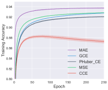
(a) MNIST, Linear

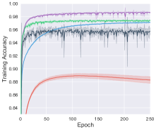
(b) MNIST, MLP

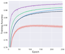
(c) Fashion-MNIST, Linear

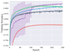
(d) Fashion-MNIST, MLP

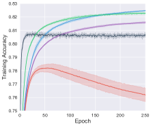
(e) Kuzushiji-MNIST, Linear

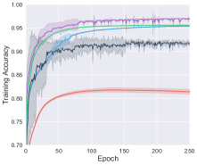
(f) Kuzushiji-MNIST, MLP

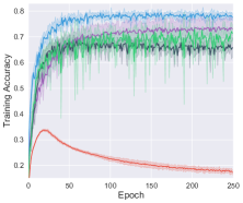
(g) CIFAR-10, Resnet

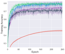
(h) CIFAR-10, Densenet

Figure 2: Experimental results of different loss functions for different datasets and models. Dark colors show the mean accuracy of 5 trials and light colors show the standard deviation.

Firstly, it is clear that each loss function is non-negative. Besides, for each loss function, the loss becomes larger if $p_{\boldsymbol{\theta}}(y|\boldsymbol{x})$ gets smaller given the correct label $y$. Note that $0<p_{\boldsymbol{\theta}}(y|\boldsymbol{x})<1$, hence the upper bound of each loss function is stated as follows.

• MAE: $\mathcal{L}_{\text{MAE}}(f(\boldsymbol{x}),y)<2$.

• MSE: $\mathcal{L}_{\text{MSE}}(f(\boldsymbol{x}),y)<1-0+\sum\nolimits_{j=1}^{k}p_{\boldsymbol{\theta}}(j|\boldsymbol{x})^{2}<2$.

• GCE: $\mathcal{L}_{\text{GCE}}(f(\boldsymbol{x}),y)<1/q$ where $q=0.7$.

• PHuber-CE: $\mathcal{L}_{\text{PHuber-CE}}(f(\boldsymbol{x}),y)<\log\tau+1$ where $\tau=10$.

Note that for CCE, $\mathcal{L}_{\text{CCE}}(f(\boldsymbol{x}),y)<-\log 0=\infty$. Therefore, we can know that MAE, MSE, GCE, and PHuber-CE are upper-bounded, while CCE is not upper-bounded.

Appendix E Additional Information of Experiments

Table 6: Classification accuracy (%) of each approach on Kuzushiji-MNIST using linear model. The best performance is highlighted in boldface.

Approach		$s=1$	$s=2$	$s=3$	$s=4$	$s=5$	$s=6$	$s=7$	$s=8$
Upper-bound Losses	EXP	60.87	62.73	63.53	64.03	64.55	65.06	65.23	65.65
		($\pm$0.38)	($\pm$0.58)	($\pm$0.30)	($\pm$0.38)	($\pm$0.41)	($\pm$0.15)	($\pm$0.10)	($\pm$0.08)
	LOG	60.11	61.57	62.71	63.36	64.01	65.68	69.35	70.10
		($\pm$0.49)	($\pm$0.15)	($\pm$0.32)	($\pm$0.09)	($\pm$0.13)	($\pm$0.27)	($\pm$0.22)	($\pm$0.18)
Bounded Losses	MAE	60.43	62.71	63.51	63.75	63.94	64.61	64.82	65.10
		($\pm$0.43)	($\pm$0.45)	($\pm$0.10)	($\pm$0.31)	($\pm$0.38)	($\pm$0.19)	($\pm$0.16)	($\pm$0.16)
	MSE	58.97	62.07	63.05	63.85	64.47	64.80	65.17	65.43
		($\pm$0.47)	($\pm$0.54)	($\pm$0.38)	($\pm$0.57)	($\pm$0.43)	($\pm$0.34)	($\pm$0.25)	($\pm$0.10)
	GCE	60.48	62.71	63.13	63.87	63.91	64.28	64.38	64.33%
		($\pm$0.55)	($\pm$0.65)	($\pm$0.30)	($\pm$0.33)	($\pm$0.30)	($\pm$0.07)	($\pm$0.12)	($\pm$0.06)
	Phuber-CE	52.69	56.58	61.10	62.32	64.51	64.93	65.96	65.81
		($\pm$4.22)	($\pm$3.94)	($\pm$2.58)	($\pm$1.50)	($\pm$0.68)	($\pm$0.52)	($\pm$0.37)	($\pm$0.62)
Unbounded Loss	CCE	51.59	55.98	59.15	61.08	63.19	65.05	66.82	68.23
		($\pm$0.64)	($\pm$1.26)	($\pm$1.18)	($\pm$0.78)	($\pm$0.54)	($\pm$0.51)	($\pm$0.41)	($\pm$0.21)
Decomposition before Shuffle	GA	51.72	53.78	54.58	54.78	55.33	55.67	55.91	56.15
		($\pm$1.04)	($\pm$1.07)	($\pm$0.87)	($\pm$0.58)	($\pm$0.29)	($\pm$0.31)	($\pm$0.42)	($\pm$0.23)
	NN	55.03	57.68	58.87	59.52	60.41	60.89	61.41	61.62
		($\pm$1.35)	($\pm$1.29)	($\pm$1.19)	($\pm$0.87)	($\pm$0.59)	($\pm$0.53)	($\pm$0.36)	($\pm$0.09)
	FREE	57.26	60.69	62.77	63.91	64.54	66.21	67.00	67.71
		($\pm$0.83)	($\pm$0.96)	($\pm$0.79)	($\pm$0.65)	($\pm$0.55)	($\pm$0.56)	($\pm$0.28)	($\pm$0.20)
	PC	54.31	58.11	60.15	61.32	62.56	63.55	64.27	65.16
		($\pm$1.04)	($\pm$0.87)	($\pm$0.79)	($\pm$0.68)	($\pm$0.59)	($\pm$0.43)	($\pm$0.20)	($\pm$0.18)
	Forward	60.05	61.53	62.43	62.98	63.48	63.95	64.14	64.27
		($\pm$0.43)	($\pm$0.31)	($\pm$0.26)	($\pm$0.40)	($\pm$0.34)	($\pm$0.29)	($\pm$0.09)	($\pm$0.16)
Decomposition after Shuffle	GA	51.72	53.79	54.59	54.83	55.33	55.67	55.90	56.18
		($\pm$1.05)	($\pm$1.07)	($\pm$0.85)	($\pm$0.58)	($\pm$0.35)	($\pm$0.31)	($\pm$0.41)	($\pm$0.22)
	NN	55.03	58.58	60.43	61.58	62.99	64.00	65.07	66.08
		($\pm$1.35)	($\pm$1.11)	($\pm$1.00)	($\pm$0.72)	($\pm$0.49)	($\pm$0.48)	($\pm$0.36)	($\pm$0.10)
	FREE	57.26	60.32	62.11	62.98	64.30	65.18	66.02	67.02
		($\pm$0.84)	($\pm$0.94)	($\pm$0.64)	($\pm$0.67)	($\pm$0.47)	($\pm$0.45)	($\pm$0.28)	($\pm$0.18)
	PC	54.31	57.32	58.95	60.17	61.47	62.54	63.53	64.74
		($\pm$1.04)	($\pm$0.76)	($\pm$0.77)	($\pm$0.83)	($\pm$0.45)	($\pm$0.40)	($\pm$0.22)	($\pm$0.22)
	Forward	60.02	61.75	62.68	63.19	63.59	63.94	64.18	64.32
		($\pm$0.44)	($\pm$0.25)	($\pm$0.23)	($\pm$0.28)	($\pm$0.19)	($\pm$0.09)	($\pm$0.14)	($\pm$0.15)

Table 7: Classification accuracy (%) of each approach on Kuzushiji-MNIST using MLP. The best performance is highlighted in boldface.

Approach		$s=1$	$s=2$	$s=3$	$s=4$	$s=5$	$s=6$	$s=7$	$s=8$
Upper-bound Losses	EXP	71.66	82.51	84.45	87.10	88.35	89.61	90.18	90.92
		($\pm$3.48 )	($\pm$3.08 )	($\pm$0.24 )	($\pm$0.37 )	($\pm$0.18 )	($\pm$0.33 )	($\pm$0.37 )	($\pm$0.15)
	LOG	77.07	82.39	85.54	87.60	88.87	89.25	90.22	91.19
		($\pm$3.00 )	($\pm$0.73 )	($\pm$0.35 )	($\pm$0.40 )	($\pm$0.34 )	($\pm$0.37 )	($\pm$0.31 )	($\pm$0.11)
Bounded Losses	MAE	69.87	73.60	79.97	85.34	86.91	89.10	90.32	91.06
		($\pm$1.04 )	($\pm$5.77 )	($\pm$3.71 )	($\pm$2.78 )	($\pm$3.06 )	($\pm$0.46 )	($\pm$0.31 )	($\pm$0.34)
	MSE	57.56	71.37	78.26	82.97	85.37	86.82	88.03	88.69
		($\pm$0.92 )	($\pm$0.89 )	($\pm$0.49 )	($\pm$0.41 )	($\pm$0.45 )	($\pm$0.13 )	($\pm$0.11 )	($\pm$0.05)
	GCE	63.85	74.11	79.18	83.65	85.23	86.32	87.12	87.64
		($\pm$1.27 )	($\pm$2.38 )	($\pm$2.31 )	($\pm$0.15 )	($\pm$0.25 )	($\pm$0.27 )	($\pm$0.20 )	($\pm$0.09)
	Phuber-CE	10.24	14.76	26.60	73.43	81.41	83.00	84.69	85.59
		($\pm$4.09 )	($\pm$2.11 )	($\pm$1.58 )	($\pm$1.50 )	($\pm$0.58 )	($\pm$0.42 )	($\pm$0.47 )	($\pm$0.52)
Unbounded Loss	CCE	56.17	60.89	64.18	66.57	69.14	71.63	74.55	78.22
		($\pm$0.64 )	($\pm$0.61 )	($\pm$0.77 )	($\pm$0.41 )	($\pm$0.49 )	($\pm$0.31 )	($\pm$0.31 )	($\pm$0.22)
Decomposition before Shuffle	GA	70.25	76.50	79.77	82.03	84.05	85.58	86.40	87.49
		($\pm$0.24 )	($\pm$0.47 )	($\pm$0.32 )	($\pm$0.22 )	($\pm$0.64 )	($\pm$0.32 )	($\pm$0.24 )	($\pm$0.15)
	NN	65.33	71.34	75.46	78.67	81.40	84.08	86.56	88.61
		($\pm$0.51 )	($\pm$0.53 )	($\pm$0.31 )	($\pm$0.58 )	($\pm$0.28 )	($\pm$0.16 )	($\pm$0.39 )	($\pm$0.12)
	FREE	53.90	60.32	63.98	66.79	69.31	71.65	74.43	76.61
		($\pm$1.05 )	($\pm$1.14 )	($\pm$0.85 )	($\pm$0.64 )	($\pm$0.73 )	($\pm$0.73 )	($\pm$0.28 )	($\pm$0.33)
	PC	56.36	62.37	66.09	69.51	72.46	75.18	78.50	82.40
		($\pm$0.56 )	($\pm$0.50 )	($\pm$0.44 )	($\pm$0.47 )	($\pm$0.35 )	($\pm$0.33 )	($\pm$0.52 )	($\pm$0.38)
	Forward	75.40	83.19	85.18	86.63	87.51	88.29	88.96	89.41
		($\pm$2.02 )	($\pm$0.61 )	($\pm$0.48 )	($\pm$0.38 )	($\pm$0.29 )	($\pm$0.29 )	($\pm$0.26 )	($\pm$0.25)
Decomposition after Shuffle	GA	70.25	75.91	78.46	80.60	82.14	83.48	84.01	84.65
		($\pm$0.24 )	($\pm$1.37 )	($\pm$2.84 )	($\pm$3.35 )	($\pm$4.51 )	($\pm$4.92 )	($\pm$5.35 )	($\pm$6.28)
	NN	63.73	67.26	69.46	71.25	73.15	74.82	77.09	79.39
		($\pm$0.97 )	($\pm$0.82 )	($\pm$0.74 )	($\pm$0.62 )	($\pm$0.45 )	($\pm$0.35 )	($\pm$0.17 )	($\pm$0.21)
	FREE	55.33	60.81	64.65	67.01	69.60	71.63	74.22	77.16
		($\pm$0.89 )	($\pm$0.97 )	($\pm$0.89 )	($\pm$0.70 )	($\pm$0.78 )	($\pm$0.46 )	($\pm$0.40 )	($\pm$0.50)
	PC	56.68	61.07	63.86	65.61	68.03	69.74	72.49	75.17
		($\pm$1.28 )	($\pm$0.99 )	($\pm$0.67 )	($\pm$0.44 )	($\pm$0.64 )	($\pm$0.65 )	($\pm$0.37 )	($\pm$0.46)
	Forward	66.09	73.20	75.76	82.53	86.27	88.05	89.24	90.22
		($\pm$0.49 )	($\pm$3.05 )	($\pm$2.61 )	($\pm$2.60 )	($\pm$0.65 )	($\pm$0.27 )	($\pm$0.22 )	($\pm$0.20)

E.1 Datasets and Models

In the experiments of Section 5, we use 5 widely-used large-scale benchmark datasets and 4 regular-scale datasets from the UCI Machine Learning Repository. The statistics of these datasets with the corresponding base models are reported in Table 5. Hyper-parameters for all the approaches are selected so as to maximize the accuracy on a validation set, which is constructed by randomly sampling 10% of the training set. We report the characteristics, the parameter settings (to reproduce the experimental results), and the sources of these datasets as follows.

• MNIST (LeCun et al., 1998): It is a 10-class dataset of handwritten digits (0 to 9). Each instance is a 28$\times$28 grayscale image. Source: http://yann.lecun.com/exdb/mnist/

• Kuzushiji-MNIST (Clanuwat et al., 2018): It is a 10-class dataset of cursive Japanese (“Kuzushiji”) characters. Each instance is a 28$\times$28 grayscale image.

• Fashion-MNIST (Xiao et al., 2017): It is a 10-class dataset of fashion items (T-shirt/top, trouser, pullover, dress, sandal, coat, shirt, sneaker, bag, and ankle boot). Each instance is a 28$\times$28 grayscale image. Source: https://github.com/rois-codh/kmnist

• CIFAR-10 (Krizhevsky et al., 2009): It is a 10-class dataset of 10 different objects (airplane, bird, automobile, cat, deer, dog, frog, horse, ship, and truck). Each instance is a 32$\times$32$\times$3 colored image in RGB format. This dataset is normalized with mean $(0.4914,0.4822,0.4465)$ and standard deviation $(0.247,0.243,0.261)$. Source: https://www.cs.toronto.edu/~kriz/cifar.html

• 20Newsgroups: It is a 20-class dataset of 20 different newsgroups (comp.graphics, comp.os.ms-windows.misc, comp.sys.ibm.pc.hardware, comp.sys.mac.hardware, comp.windows.x, rec.autos, rec.motorcycles, rec.sport.baseball, rec.sport.hockey, sci.crypt, sci.electronics, sci.med, sci.space, misc.forsale, talk.politics.misc, talk.politics.guns, talk.politics.mideast, talk.religion.misc, alt.atheism, soc.religion.christian). We obtained the tf-idf features, and applied TruncatedSVD (Halko et al., 2011) to reduce the dimension to 1000. We randomly sample 90% of the examples from the whole dataset to construct the training set, and the rest 10% forms the test set. Source: http://qwone.com/~jason/20Newsgroups/

• Yeast, Texture, Dermatology, Synthetic Control: They are all the datasets from the UCI Machine Learning Repository. Since they are all regular-scale datasets, we only apply linear model on them. For each dataset, we randomly sample 90% of the examples from the whole dataset to construct the training set, and the rest 10% forms the test set. The detailed parameter settings can be found in our provided code package. Source: https://archive.ics.uci.edu/ml/datasets.php

For the used models, the detailed information of the used 34-layer ResNet (He et al., 2016) and 22-layer DenseNet (Huang et al., 2017) can be found in the corresponding papers.

E.2 Experimental Results on Training Accuracy

Here, we report the mean and standard deviation of training accuracy (the training set is evaluated with ordinary labels) of 5 trials in Figure 2, to compare the bounded loss functions MAE, MSE, GCE, PHuber-CE, and the unbounded loss function CCE. The training accuracy can reflect the ability of the loss function in identifying the correct label from the non-complementary labels.

From Figure 2, we can find that CCE always achieves the worst performance among all the loss functions, which implies that unbounded loss function is worse than bounded loss function, using our provided empirical risk estimator. This observation clearly supports our conjecture that the negative term in our empirical risk estimator could cause the over-fitting issue. In addition, we can also find that compared with other bounded loss functions, MAE achieves comparable performance in most cases, while it is sometimes inferior to other bounded losses due to its optimization issue (Zhang & Sabuncu, 2018). All the above observations on the training accuracy (Figure 2) are very similar to those observations on the test accuracy (Figure 1 in our paper).

E.3 Experimental Results on Fixed Complementary Label Set

We also conduct additional experiments to investigate the influence of the variable $s$ on Kuzushiji-MNIST using both linear model and MLP. Specifically, we study the case where the size of each complementary label set $s$ is fixed at $j$ (i.e., $p(s=j)=1$) while increasing $j$ from 1 to $k-2$. The detailed experimental results are shown in Table 6 and Table 7. From the two tables, we can find that the (test) classification accuracy of our approaches increases as $j$ increases. This observation is clearly in accordance with our derived estimation error bound (Theorem 4), as the estimation error would decrease if $j$ increases. In addition, as shown in the two tables, our proposed upper-bound losses outperform other approaches in most cases. This observation also demonstrates the effectiveness of our proposed upper-bound losses.

References

• Bao et al. (2018) Bao, H., Niu, G., and Sugiyama, M. Classification from pairwise similarity and unlabeled data. In ICML, pp.  452–461, 2018.
• Bartlett & Mendelson (2002) Bartlett, P. L. and Mendelson, S. Rademacher and gaussian complexities: Risk bounds and structural results. JMLR, 3(11):463–482, 2002.
• Blake & Merz (1998) Blake, C. L. and Merz, C. J. Uci repository of machine learning databases, 1998. URL http://archive.ics.uci.edu/ml/index.php.
• Chapelle et al. (2006) Chapelle, O., Scholkopf, B., and Zien, A. Semi-Supervised Learning. MIT Press, 2006.
• Clanuwat et al. (2018) Clanuwat, T., Bober-Irizar, M., Kitamoto, A., Lamb, A., Yamamoto, K., and Ha, D. Deep learning for classical japanese literature. arXiv preprint arXiv:1812.01718, 2018.
• Cour et al. (2011) Cour, T., Sapp, B., and Taskar, B. Learning from partial labels. JMLR, 12(5):1501–1536, 2011.
• du Plessis et al. (2014) du Plessis, M. C., Niu, G., and Sugiyama, M. Analysis of learning from positive and unlabeled data. In NeurIPS, pp.  703–711, 2014.
• du Plessis et al. (2015) du Plessis, M. C., Niu, G., and Sugiyama, M. Convex formulation for learning from positive and unlabeled data. In ICML, pp.  1386–1394, 2015.
• Elkan & Noto (2008) Elkan, C. and Noto, K. Learning classifiers from only positive and unlabeled data. In KDD, pp.  213–220, 2008.
• Feng & An (2018) Feng, L. and An, B. Leveraging latent label distributions for partial label learning. In IJCAI, pp.  2107–2113, 2018.
• Feng & An (2019a) Feng, L. and An, B. Partial label learning with self-guided retraining. In AAAI, pp.  3542–3549, 2019a.
• Feng & An (2019b) Feng, L. and An, B. Partial label learning by semantic difference maximization. In IJCAI, pp.  2294–2300, 2019b.
• Ghosh et al. (2017) Ghosh, A., Kumar, H., and Sastry, P. Robust loss functions under label noise for deep neural networks. In AAAI, 2017.
• Halko et al. (2011) Halko, N., Martinsson, P.-G., and Tropp, J. A. Finding structure with randomness: Probabilistic algorithms for constructing approximate matrix decompositions. SIAM Review, 53(2):217–288, 2011.
• Han et al. (2018a) Han, B., Yao, J., Niu, G., Zhou, M., Tsang, I., Zhang, Y., and Sugiyama, M. Masking: A new perspective of noisy supervision. In NeurIPS, pp.  5836–5846, 2018a.
• Han et al. (2018b) Han, B., Yao, Q., Yu, X., Niu, G., Xu, M., Hu, W., Tsang, I., and Sugiyama, M. Co-teaching: Robust training of deep neural networks with extremely noisy labels. In NeurIPS, pp.  8527–8537, 2018b.
• He et al. (2016) He, K., Zhang, X., Ren, S., and Sun, J. Deep residual learning for image recognition. In CVPR, pp.  770–778, 2016.
• Huang et al. (2017) Huang, G., Liu, Z., Van Der Maaten, L., and Weinberger, K. Q. Densely connected convolutional networks. In CVPR, pp.  4700–4708, 2017.
• Ishida et al. (2017) Ishida, T., Niu, G., Hu, W., and Sugiyama, M. Learning from complementary labels. In NeurIPS, pp.  5644–5654, 2017.
• Ishida et al. (2018) Ishida, T., Niu, G., and Sugiyama, M. Binary classification for positive-confidence data. In NeurIPS, pp.  5917–5928, 2018.
• Ishida et al. (2019) Ishida, T., Niu, G., Menon, A. K., and Sugiyama, M. Complementary-label learning for arbitrary losses and models. In ICML, pp.  2971–2980, 2019.
• Kaneko et al. (2019) Kaneko, T., Sato, I., and Sugiyama, M. Online multiclass classification based on prediction margin for partial feedback. arXiv preprint arXiv:1902.01056, 2019.
• Kingma & Ba (2015) Kingma, D. P. and Ba, J. Adam: A method for stochastic optimization. In ICLR, 2015.
• Kiryo et al. (2017) Kiryo, R., Niu, G., du Plessis, M. C., and Sugiyama, M. Positive-unlabeled learning with non-negative risk estimator. In NeurIPS, pp.  1674–1684, 2017.
• Krizhevsky et al. (2009) Krizhevsky, A., Hinton, G., et al. Learning multiple layers of features from tiny images. Technical report, Citeseer, 2009.
• Lang (1995) Lang, K. Newsweeder: Learning to filter netnews. In ICML, 1995.
• LeCun et al. (1998) LeCun, Y., Bottou, L., Bengio, Y., Haffner, P., et al. Gradient-based learning applied to document recognition. Proceedings of the IEEE, 86(11):2278–2324, 1998.
• Li & Liang (2019) Li, Y.-F. and Liang, D.-M. Safe semi-supervised learning: a brief introduction. Frontiers of Computer Science, 13(4):669–676, 2019.
• Lu et al. (2019) Lu, N., Niu, G., Menon, A. K., and Sugiyama, M. On the minimal supervision for training any binary classifier from only unlabeled data. In ICLR, 2019.
• Lu et al. (2020) Lu, N., Zhang, T., Niu, G., and Sugiyama, M. Mitigating overfitting in supervised classification from two unlabeled datasets: A consistent risk correction approach. In AISTATS, 2020.
• Maurer (2016) Maurer, A. A vector-contraction inequality for rademacher complexities. In ALT, pp.  3–17, 2016.
• McDiarmid (1989) McDiarmid, C. On the method of bounded differences. In Surveys in Combinatorics, 1989.
• Menon et al. (2015) Menon, A., Van Rooyen, B., Ong, C. S., and Williamson, B. Learning from corrupted binary labels via class-probability estimation. In ICML, pp.  125–134, 2015.
• Menon et al. (2020) Menon, A. K., Rawat, A. S., Reddi, S. J., and Kumar, S. Can gradient clipping mitigate label noise? In ICLR, 2020.
• Miyato et al. (2018) Miyato, T., Maeda, S.-i., Koyama, M., and Ishii, S. Virtual adversarial training: a regularization method for supervised and semi-supervised learning. TPAMI, 41(8):1979–1993, 2018.
• Mohri et al. (2012) Mohri, M., Rostamizadeh, A., and Talwalkar, A. Foundations of Machine Learning. MIT Press, 2012.
• Niu et al. (2013) Niu, G., Jitkrittum, W., Dai, B., Hachiya, H., and Sugiyama, M. Squared-loss mutual information regularization: A novel information-theoretic approach to semi-supervised learning. In ICML, pp.  10–18, 2013.
• Rezaei et al. (2019) Rezaei, M., Yang, H., and Meinel, C. Recurrent generative adversarial network for learning imbalanced medical image semantic segmentation. Multimedia Tools and Applications, pp.  1–20, 2019.
• Sakai et al. (2017) Sakai, T., du Plessis, M. C., Niu, G., and Sugiyama, M. Semi-supervised classification based on classification from positive and unlabeled data. In ICML, pp.  2998–3006, 2017.
• Sakai et al. (2018) Sakai, T., Niu, G., and Sugiyama, M. Semi-supervised auc optimization based on positive-unlabeled learning. MLJ, 107(4):767–794, 2018.
• Wang et al. (2019) Wang, X., Kodirov, E., Hua, Y., and Robertson, N. M. Improving mae against cce under label noise. arXiv preprint arXiv:1903.12141, 2019.
• Wei et al. (2020) Wei, H., Feng, L., Chen, X., and An, B. Combating noisy labels by agreement: A joint training method with co-regularization. In CVPR, June 2020.
• Xia et al. (2019) Xia, X., Liu, T., Wang, N., Han, B., Gong, C., Niu, G., and Sugiyama, M. Are anchor points really indispensable in label-noise learning? In NeurIPS, pp.  6835–6846, 2019.
• Xiao et al. (2017) Xiao, H., Rasul, K., and Vollgraf, R. Fashion-mnist: a novel image dataset for benchmarking machine learning algorithms. arXiv preprint arXiv:1708.07747, 2017.
• Yu et al. (2018) Yu, X., Liu, T., Gong, M., and Tao, D. Learning with biased complementary labels. In ECCV, pp.  68–83, 2018.
• Zhang & Yu (2015) Zhang, M.-L. and Yu, F. Solving the partial label learning problem: An instance-based approach. In IJCAI, pp.  4048–4054, 2015.
• Zhang (2004) Zhang, T. Statistical analysis of some multi-category large margin classification methods. JMLR, 5(10):1225–1251, 2004.
• Zhang & Sabuncu (2018) Zhang, Z. and Sabuncu, M. Generalized cross entropy loss for training deep neural networks with noisy labels. In NeurIPS, pp.  8778–8788, 2018.
• Zhou (2018) Zhou, Z. A brief introduction to weakly supervised learning. National Science Review, 5(1):44–53, 2018.
• Zhu & Goldberg (2009) Zhu, X. and Goldberg, A. B. Introduction to semi-supervised learning. Synthesis Lectures on Artificial Intelligence and Machine Learning, 3(1):1–130, 2009.