Soft corrections to inclusive deep-inelastic scattering at four loops and beyond

Abstract

We study the threshold corrections for inclusive deep-inelastic scattering (DIS) and their all-order resummation. Using recent results for the QCD form factor, related anomalous dimensions and Mellin moments of DIS structure functions at four loops we derive the complete soft and collinear contributions to the DIS Wilson coefficients at four loops. For a general $SU(n_{c})$ gauge group the results are exact in the large-$n_{c}$ approximation and for QCD with $n_{c}=3$ we present precise approximations. We extend the threshold resummation exponent $G^{N}$ in Mellin-$N$ space to the fifth logarithmic (N${}^{4}$LL) order collecting the terms $\alpha_{\rm s}^{\,3}(\alpha_{\rm s}\ln N)^{n}$ to all orders in the strong coupling constant $\alpha_{\rm s}$. We study the numerical effect of the N${}^{4}$LL corrections using both the fully exponentiated form and the expansion of the coefficient function in towers of logarithms. As a byproduct, we derive a numerical result for the complete pole structure of the QCD form factor in the parameter of dimensional regularization $\varepsilon$ at four loops.

1 Introduction

The cross section for inclusive deep-inelastic scattering (DIS) of charged leptons or neutrinos off a nucleon target can be expressed in terms of structure functions, which factorize into the product of operator matrix elements for the nucleon under consideration and the DIS Wilson coefficients. The latter parametrize the hard partonic scattering cross section driven by short-distance physics and are calculable in perturbative Quantum Chromodynamics (QCD) order by order in the strong coupling constant $\alpha_{\rm s}$. However, only a few terms in this expansion can be calculated completely. Currently, the QCD corrections at next-to-next-to-next-to-leading order (N${}^{3}$LO) for the neutral- and charged-current DIS structure functions $F_{1}$, $F_{2}$ and $F_{3}$ are known Vermaseren:2005qc; Moch:2008fj. In the exceptional region of phase space, on the other hand, when the Bjorken scaling variable $x$ is close to unity, $x\to 1$, the DIS Wilson coefficients develop large Sudakov logarithms at all orders in the form $\alpha_{\rm s}^{n}\ln^{l}(1-x)/(1-x)_{+}$, with $l=2n-1,\dots,0$. These are a consequence of the constrained phase space available for the real emission of soft and collinear gluons.

The DIS Wilson coefficients are subject to an additional factorization for $x\to 1$ (or $N\to\infty$ in Mellin-$N$ space) which allows for resummation of those Sudakov double logarithms Sterman:1986aj; Catani:1989ne; Catani:1990rp; Catani:1996yz; Contopanagos:1996nh. Based on the fixed-order QCD results up to N${}^{3}$LO for the DIS structure functions Vermaseren:2005qc; Moch:2008fj this resummation has been performed to next-to-next-to-next-to-leading logarithmic (N${}^{3}$LL) accuracy in Mellin-$N$ space Moch:2005ba, where the resummation takes the form of an exponentiation which organizes the respective logarithms $\alpha_{\rm s}^{n}\ln^{l}N$, with $l=2n,\dots,1$ (see also Manohar:2003vb; Chay:2005rz; Idilbi:2006dg; Becher:2006mr for related work in the Soft-Collinear Effective Theory).

From a phenomenological point of view, resummation in DIS is essential to obtain reliable QCD predictions in the (small) region of phase space dominated by such large threshold logarithms. This is of particular relevance since DIS structure functions also receive power corrections beyond the QCD factorization at leading twist and such higher-twist contributions are supposed to be significant at large $x$. Therefore, good control of the perturbative series at leading twist is important to distinguish those effects in the analyses of DIS data, see for instance Accardi:2016ndt.

From a field-theoretic point of view, on the other hand, the threshold limit in DIS is of interest, since the factorization of the DIS Wilson coefficients for $x\to 1$ links a number of fundamental quantities in QCD with each other due to the universality of the soft and collinear limit. In particular, this comprises the QCD form factor which features an all-order exponentiation in dimensional regularization with $d=4-2\varepsilon$ dimensions Collins:1980ih; Sen:1981sd; Korchemsky:1988hd; Magnea:1990zb; Magnea:2000ss; Moch:2005id and the QCD splitting functions, currently fully known to next-to-next-to-leading order (NNLO) Moch:2004pa; Vogt:2004mw. The necessary cancellation of soft and collinear singularities in $\varepsilon$ in inclusive observables due to the Kinoshita-Lee-Nauenberg theorem Kinoshita:1962ur; Lee:1964is offers a constructive approach to the DIS Wilson coefficients near threshold Moch:2005ky, see also Laenen:2005uz; Ravindran:2005vv; Ravindran:2006cg.

Recent progress in the computation of QCD corrections has been obtained in particular for the quark form factor Lee:2016ixa and the non-singlet quark splitting functions Moch:2017uml, which have been calculated at four-loop order in the limit of large-${n_{c}}$ for a general $SU({n_{c}})$ gauge group. In addition, a low number of fixed Mellin moments for the DIS structure functions are available at four loops Ruijl:2016pkm, as well as information on the ${n_{\!f}}$-dependence of the QCD form factor Ruijl:2016pkm; Lee:2017mip; Grozin:2018vdn; Henn:2019rmi; Bruser:2019auj and on new colour factors (quartic Casimirs) Moch:2018wjh; Henn:2019rmi; Lee:2019zop; vonManteuffel:2019wbj; Henn:2019swt; Huber:2019fxe. Taken together Das:2019uvh, these results allow us to extend the threshold resummation exponent $G^{N}$ for DIS Wilson coefficients in Mellin-$N$ space to the fifth logarithmic (N${}^{4}$LL) order. At this accuracy we collect and resum in $G^{N}$ the terms $\alpha_{\rm s}^{\,3}(\alpha_{\rm s}\ln N)^{n}$ to all orders in $\alpha_{\rm s}$. To that end, we extract the resummation exponent $B^{\rm DIS}$ of the quark jet function collecting final-state collinear emissions at the fourth order in $\alpha_{\rm s}$, and we address the term $\alpha_{\rm s}^{4}/(1-x)_{+}$ in the fixed-order expansion of the DIS Wilson coefficients at four loops. With the help of the available four-loop QCD results, we can provide exact expressions in the large-${n_{c}}$ limit and adequate numerical approximations for full QCD with ${n_{c}}=3$. As a byproduct, we also derive a numerical result including full colour dependence for the single pole $1/\varepsilon$ of the dimensional regulated QCD form factor at four loops.

This article is organized as follows. In Sec. 2 we recall the general structure of the threshold resummation for DIS and provide the required formulae to perform resummation to N${}^{4}$LL accuracy. In Sec. 3 we describe the extraction of the resummation coefficients and the calculation of the DIS Wilson coefficient in the soft and collinear limit. We present a numerical study for the exponentiated resummed DIS Wilson coefficients and their tower expansion in Sec. 4 and summarize in Sec. 5. Exact expressions for the DIS Wilson coefficients are given in Appendix A.

2 Theoretical framework

The general structure of the resummed DIS Wilson coefficients takes the following form in the Mellin $N$-space Sterman:1986aj; Catani:1989ne,

$$C_{a,q}^{\,N}(Q^{2})\>=\>g_{0}^{a}(Q^{2})\cdot\exp\,[G^{N}(Q^{2})]\>+\>{\cal O}(N^{-1}\ln^{n}N)\>\>,$$ (2.1)

for the neutral- or charged-current DIS structure functions $F_{a}$, where $a=1,2,3$. In Mellin space they factorize in a sum over all partons $i$ as $F_{a}^{\,N}(Q^{2})=C_{a,i}^{\,N}(Q^{2})f_{i}^{\,N}$ with $f_{i}^{\,N}$ denoting the Mellin transformed parton distributions $f_{i}(x)$ for the parton $i$, and the Born contributions to the are normalized as $C_{a,q}^{\,N}|_{\rm LO}=1$. Here the resummation exponent $G^{N}$ contains all terms of the form $\ln^{\,k}N$ to all orders in $\alpha_{\rm s}$, and the pre-factor $g_{0}$ encompasses the $N$- independent terms. $G^{N}$ and $g_{0}$ depend on the physical hard scale $Q^{2}$ ($\,=-q^{2}$ in DIS, with $q$ the four-momentum of the exchanged gauge boson), and on the renormalization and factorization scales $\mu$ and $\mu_{f}$, suppressed for brevity. For inclusive DIS $G^{N}$ reads in the notation of Catani:1998tm; Moch:2005ba

$$G^{N}\;\; = \ln\Delta_{\,\rm q}\>+\>\ln J_{\rm q}\>+\>\ln\Delta^{\,\rm int}_{\,\rm DIS}\>\>,$$ (2.2)

where the radiation factors ($\Delta_{\,\rm q},J_{\rm q},\Delta^{\,\rm int}_{\,\rm DIS}$) are given by well-known integrals over functions of the running coupling. The collinear soft-gluon radiation off an initial-state quark is collected by

$$\ln\Delta_{\,\rm q}(Q^{2},\,\mu_{\!f}^{\>\!2})\>=\>\int_{0}^{1}\!dz\,\frac{z^{N-1}-1}{1-z}\,\int_{\mu_{\!f}^{\>\!2}}^{(1-z)^{2}Q^{2}}\frac{dq^{2}}{q^{2}}\,A^{\rm q}(\alpha_{\rm s}(q^{2}))\>\>,$$ (2.3)

with the light-like cusp anomalous dimension $A^{\rm q}(\alpha_{\rm s})$ addressed below. The collinear emissions from an ‘unobserved’ final-state quark are summarized in the jet function,

$$\ln J_{\rm q}(Q^{2})\>=\>\int_{0}^{1}\!dz\,\frac{z^{N-1}-1}{1-z}\,\left[\int_{(1-z)^{2}Q^{2}}^{(1-z)Q^{2}}\frac{dq^{2}}{q^{2}}\,A^{\rm q}(\alpha_{\rm s}(q^{2}))+B^{\rm DIS}(\alpha_{\rm s}([1-z]Q^{2}))\right]$$ (2.4)

including the additional function $B^{\rm DIS}(\alpha_{\rm s})$. All expansions in terms of the strong coupling $\alpha_{\rm s}$ are normalized as

$$A^{\rm q}(\alpha_{\rm s})\,=\,\sum_{n=1}^{\infty}\left(\frac{\alpha_{\rm s}}{4\pi}\right)^{n}\,A_{n}\,\equiv\,\sum_{n=1}^{\infty}a_{\rm s}^{n}\,A_{n}$$ (2.5)

etc. Any process-dependent contributions from large-angle soft gluons emissions are contained in the function $\Delta^{\rm int}_{\rm DIS}$ which, however, evaluates to unity, i.e., $\Delta^{\rm int}_{\rm DIS}=1$, since the corresponding evolution kernels vanish at all order in $\alpha_{\rm s}$ for inclusive DIS Forte:2002ni; Gardi:2002xm. Thus, the last term in eq. (2.2) is absent for inclusive DIS. The running of the strong coupling is governed by the QCD beta function

$$\beta(a_{\rm s})=-\sum_{n=0}^{\infty}a_{\rm s}^{n+2}\,\beta_{n}\,,$$ (2.6)

with $\beta_{0}=(11/3){C_{\!A}}-(2/3){n_{\!f}}$ and so on.

The evaluation of the integrals in eqs. (2.3) and (2.4) proceeds in a standard manner, see for instance Moch:2005ba; Catani:2003zt, leading to the following expression of the resummation exponent $G^{N}$,

$$G^{N}=\ln\widetilde{N}g_{1}^{\rm DIS}(\lambda)+g_{2}^{\rm DIS}(\lambda)+a_{\rm s}g_{3}^{\rm DIS}(\lambda)+a_{\rm s}^{2}g_{4}^{\rm DIS}(\lambda)+a_{\rm s}^{3}g_{5}^{\rm DIS}(\lambda)\,,$$ (2.7)

where $\lambda=\beta_{0}a_{\rm s}\ln\widetilde{N}$ with $\widetilde{N}=N\exp(\gamma_{E})$, where $\gamma_{E}\simeq 0.57721566$ is the Euler-Mascheroni constant. The number of terms on the right hand side of $G^{N}$ provides the resummation accuracy, namely LL, NLL …, respectively. For notational brevity we have organized the logarithms in Mellin space as $\ln\widetilde{N}$. Eq. (2.7) is accurate to N${}^{4}$LL order and the coefficient $g_{5}^{\,\rm DIS}(\lambda)$ collects all large logarithms up to $\alpha_{\rm s}^{\,3}(\alpha_{\rm s}\ln\widetilde{N})^{n}$ in $G^{N}$. The complete results for $g_{i}^{\rm DIS}$ with $i\leq 5$, including for consistency the well-known lower order results Sterman:1986aj; Catani:1989ne; Vogt:2000ci; Catani:2003zt; Moch:2005ba, read

$$g_{1}^{\,\rm DIS}(\lambda) = (1+\lambda^{-1}\*L_{\lambda_{1}}-L_{\lambda_{1}})\*A_{1}\>\>,$$

$$g_{2}^{\,\rm DIS}(\lambda) = -(L_{\lambda_{1}}+\lambda)\*A_{2}+L_{\lambda_{1}}\*B^{\rm DIS}_{1}+(L_{\lambda_{1}}+L_{\lambda_{1}}^{2}/2+\lambda)\*A_{1}\*\beta_{1}+L_{\,\rm qr\,}\*L_{\lambda_{1}}\*A_{1}+L_{\,\rm fr\,}\*\lambda\*A_{1}\>\>,$$

$$g_{3}^{\,\rm DIS}(\lambda) = -(1-\lambda_{1}^{-1}+\lambda)\*A_{3}/2+(1-\lambda_{1}^{-1})\*(B^{\rm DIS}_{2}-A_{1}\*\zeta_{2}/2)$$

$$\mbox{}-(1-\lambda_{1}^{-1}-2\*\lambda_{1}^{-1}\*L_{\lambda_{1}}-\lambda_{1}^{-1}\*L_{\lambda_{1}}^{2}+2\*L_{\lambda_{1}}+\lambda)\*A_{1}\*\beta_{1}^{2}/2$$

$$\mbox{}-(1-\lambda_{1}^{-1}-\lambda_{1}^{-1}\*L_{\lambda_{1}})\*B^{\rm DIS}_{1}\*\beta_{1}+(3-3\*\lambda_{1}^{-1}-2\*\lambda_{1}^{-1}\*L_{\lambda_{1}}+\lambda)\*A_{2}\*\beta_{1}/2$$

$$\mbox{}-(1-\lambda_{1}^{-1}-2\*L_{\lambda_{1}}-\lambda)\*A_{1}\*\beta_{2}/2$$

$$\mbox{}+L_{\,\rm qr\,}\*\bigl{\{}(1-\lambda_{1}^{-1})\*(A_{2}-B^{\rm DIS}_{1})-(1-\lambda_{1}^{-1}-\lambda_{1}^{-1}\*L_{\lambda_{1}})\*A_{1}\*\beta_{1}\bigr{\}}$$

$$\mbox{}-L_{\,\rm qr\,}^{\,2}\*(1-\lambda_{1}^{-1})\*A_{1}/2+L_{\,\rm fr\,}\*\lambda\*A_{2}-L_{\,\rm fr\,}^{\,2}\*\lambda\*A_{1}/2\>\>,$$

$$g_{4}^{\rm DIS}(\lambda) = -(1-\lambda_{1}^{-2}+2\*\lambda)\*A_{4}/6+(1-\lambda_{1}^{-2})\*(B^{\rm DIS}_{3}/2+B^{\rm DIS}_{1}\*\zeta_{2}/2-A_{2}\*\zeta_{2}/2-A_{1}\*\zeta_{3}/3)$$ (2.8)

$$\mbox{}-(1-\lambda_{1}^{-2}-2\*\lambda_{1}^{-2}\*L_{\lambda_{1}})\*B^{\rm DIS}_{2}\*\beta_{1}/2+(5-5\*\lambda_{1}^{-2}-6\*\lambda_{1}^{-2}\*L_{\lambda_{1}}+4\*\lambda)\*A_{3}\*\beta_{1}/12$$

$$\mbox{}-(11+\lambda_{1}^{-2}-6\*\lambda_{1}^{-2}\*L_{\lambda_{1}}-6\*\lambda_{1}^{-2}\*L_{\lambda_{1}}^{2}-12\*\lambda_{1}^{-1}+4\*\lambda)\*A_{2}\*\beta_{1}^{2}/12$$

$$\mbox{}-\lambda_{1}^{-2}\*L_{\lambda_{1}}\*A_{1}\*\beta_{1}\*\zeta_{2}/2-(1-\lambda_{1}^{-2}-6\*L_{\lambda_{1}}-4\*\lambda)\*A_{1}\*\beta_{3}/12$$

$$\mbox{}+(2+\lambda_{1}^{-2}-3\*\lambda_{1}^{-1}+\lambda)\*A_{2}\*\beta_{2}/3+(2+\lambda_{1}^{-2}+3/2\*\lambda_{1}^{-2}\*L_{\lambda_{1}}$$

$$\mbox{}-1/2\*\lambda_{1}^{-2}\*L_{\lambda_{1}}^{3}-3\*\lambda_{1}^{-1}-3\*\lambda_{1}^{-1}\*L_{\lambda_{1}}+3/2\*L_{\lambda_{1}}+\lambda)\*A_{1}\*\beta_{1}^{3}/3$$

$$\mbox{}-(7+5\*\lambda_{1}^{-2}+6\*\lambda_{1}^{-2}\*L_{\lambda_{1}}-12\*\lambda_{1}^{-1}-12\*\lambda_{1}^{-1}\*L_{\lambda_{1}}+12\*L_{\lambda_{1}}+8\*\lambda)\*A_{1}\*\beta_{1}\*\beta_{2}/12$$

$$\mbox{}+(1+\lambda_{1}^{-2}-\lambda_{1}^{-2}\*L_{\lambda_{1}}^{2}-2\*\lambda_{1}^{-1})\*B^{\rm DIS}_{1}\*\beta_{1}^{2}/2-(1+\lambda_{1}^{-2}-2\*\lambda_{1}^{-1})\*B^{\rm DIS}_{1}\*\beta_{2}/2$$

$$\mbox{}+L_{\,\rm qr\,}\*\bigl{\{}(1-\lambda_{1}^{-2})\*(A_{3}/2-B^{\rm DIS}_{2}+A_{1}\*\zeta_{2}/2)-(1-\lambda_{1}^{-2}-2\*\lambda_{1}^{-2}\*L_{\lambda_{1}})\*A_{2}\*\beta_{1}/2$$

$$\mbox{}+(1+\lambda_{1}^{-2}-\lambda_{1}^{-2}\*L_{\lambda_{1}}^{2}-2\*\lambda_{1}^{-1})\*A_{1}\*\beta_{1}^{2}/2-(1+\lambda_{1}^{-2}-2\*\lambda_{1}^{-1})\*A_{1}\*\beta_{2}/2$$

$$\mbox{}-\lambda_{1}^{-2}\*L_{\lambda_{1}}\*B^{\rm DIS}_{1}\*\beta_{1}\bigr{\}}-L_{\,\rm qr\,}^{\,2}\*\bigl{\{}(1-\lambda_{1}^{-2})\*(A_{2}/2-B^{\rm DIS}_{1}/2)+(\lambda_{1}^{-2}\*L_{\lambda_{1}})\*A_{1}\*\beta_{1}/2\bigr{\}}$$

$$\mbox{}+L_{\,\rm qr\,}^{\,3}\*(1-\lambda_{1}^{-2})\*A_{1}/6+L_{\,\rm fr\,}\*\lambda\*A_{3}-L_{\,\rm fr\,}^{\,2}\*\lambda\*(A_{2}+A_{1}\*\beta_{1}/2)+L_{\,\rm fr\,}^{\,3}\*\lambda\*A_{1}/3\,.$$

For brevity, we use here the short-hand notations $\lambda_{1}=1-\lambda$, $L_{\lambda_{1}}=\ln(1-\lambda)$, $L_{\rm qr}=\ln(Q^{2}/\mu^{\,2})$ and $\,L_{\rm fr}=\ln(\mu_{f}^{\,2}/\mu^{\,2})\,$. Also we suppress factors of $\beta_{0}$ which can be restored easily by the substitutions $A_{k}\rightarrow A_{k}/\beta_{0}^{\,k}$, $B^{\rm DIS}_{k}\rightarrow B^{\rm DIS}_{k}/\beta_{0}^{\,k}$ and $\beta_{k}\rightarrow\beta_{k}/\beta_{0}^{\,k+1}$. In addition, $g_{3}$ needs to be multiplied by $\beta_{0}$ and $g_{4}$ by $\beta_{0}^{\,2}$.

The new function $g_{5}$ (computed with methods of Moch:2005ba and to be multiplied by $\beta_{0}^{\,3}$) is given by

$$g_{5}^{\rm DIS}(\lambda)\,\,=\,\,$$ (2.9)

$$(1-\lambda_{1}^{-3})\*(B^{\rm DIS}_{4}/3+B^{\rm DIS}_{2}\*\zeta_{2}+2\*B^{\rm DIS}_{1}\*\zeta_{3}/3-A_{3}\*\zeta_{2}/2-2\*A_{2}\*\zeta_{3}/3-9\*A_{1}\*\zeta_{4}/8)$$

$$\mbox{}-(1-\lambda_{1}^{-3}+3\*\lambda)\*A_{5}/12+(1-\lambda_{1}^{-3}+2\*\lambda_{1}^{-3}\*L_{\lambda_{1}})\*(B^{\rm DIS}_{1}\*\beta_{1}\*\zeta_{2}/2-A_{1}\*\beta_{1}\*\zeta_{3}/3)$$

$$\mbox{}-(1-\lambda_{1}^{-3}-3\*\lambda_{1}^{-3}\*L_{\lambda_{1}})\*B^{\rm DIS}_{3}\*\beta_{1}/3+(7-7\*\lambda_{1}^{-3}-12\*\lambda_{1}^{-3}\*L_{\lambda_{1}}+9\*\lambda)\*A_{4}\*\beta_{1}/36$$

$$\mbox{}-(1-\lambda_{1}^{-3}-12\*L_{\lambda_{1}}-9\*\lambda)\*A_{1}\*\beta_{4}/36+(5+\lambda_{1}^{-3}-6\*\lambda_{1}^{-1}+3\*\lambda)\*A_{2}\*\beta_{3}/12$$

$$\mbox{}-(5-5\*\lambda_{1}^{-3}+18\*\lambda_{1}^{-2}-18\*\lambda_{1}^{-1}+12\*L_{\lambda_{1}}+9\*\lambda)\*A_{1}\*\beta_{2}^{2}/36$$

$$\mbox{}-(7-\lambda_{1}^{-3}+2\*\lambda_{1}^{-3}\*L_{\lambda_{1}}+6\*\lambda_{1}^{-3}\*L_{\lambda_{1}}^{2}+2\*\lambda_{1}^{-3}\*L_{\lambda_{1}}^{3}-\lambda_{1}^{-3}\*L_{\lambda_{1}}^{4}+6\*\lambda_{1}^{-2}-6\*\lambda_{1}^{-2}\*L_{\lambda_{1}}^{2}-12\*\lambda_{1}^{-1}$$

$$\mbox{}-6\*\lambda_{1}^{-1}\*L_{\lambda_{1}}+4\*L_{\lambda_{1}}+3\*\lambda)\*A_{1}\*\beta_{1}^{4}/12+(41-5\*\lambda_{1}^{-3}+12\*\lambda_{1}^{-3}\*L_{\lambda_{1}}+18\*\lambda_{1}^{-3}\*L_{\lambda_{1}}^{2}+36\*\lambda_{1}^{-2}$$

$$\mbox{}-18\*\lambda_{1}^{-2}\*L_{\lambda_{1}}^{2}-72\*\lambda_{1}^{-1}-36\*\lambda_{1}^{-1}\*L_{\lambda_{1}}+36\*L_{\lambda_{1}}+27\*\lambda)\*A_{1}\*\beta_{1}^{2}\*\beta_{2}/36$$

$$\mbox{}-(2+\lambda_{1}^{-3}-3\*\lambda_{1}^{-1})\*B^{\rm DIS}_{1}\*\beta_{3}/6+(1+\lambda_{1}^{-3}-2\*\lambda_{1}^{-2}+\lambda)\*A_{3}\*\beta_{2}/4$$

$$\mbox{}-(7+2\*\lambda_{1}^{-3}+3\*\lambda_{1}^{-3}\*L_{\lambda_{1}}-9\*\lambda_{1}^{-1}-9\*\lambda_{1}^{-1}\*L_{\lambda_{1}}+12\*L_{\lambda_{1}}+9\*\lambda)\*A_{1}\*\beta_{1}\*\beta_{3}/18$$

$$\mbox{}-(20+7\*\lambda_{1}^{-3}+12\*\lambda_{1}^{-3}\*L_{\lambda_{1}}-9\*\lambda_{1}^{-2}-18\*\lambda_{1}^{-2}\*L_{\lambda_{1}}-18\*\lambda_{1}^{-1}+9\*\lambda)\*A_{2}\*\beta_{1}\*\beta_{2}/18$$

$$\mbox{}-(13+5\*\lambda_{1}^{-3}-12\*\lambda_{1}^{-3}\*L_{\lambda_{1}}-18\*\lambda_{1}^{-3}\*L_{\lambda_{1}}^{2}-18\*\lambda_{1}^{-2}+9\*\lambda)\*A_{3}\*\beta_{1}^{2}/36$$

$$\mbox{}+(25+11\*\lambda_{1}^{-3}+24\*\lambda_{1}^{-3}\*L_{\lambda_{1}}-12\*\lambda_{1}^{-3}\*L_{\lambda_{1}}^{3}-18\*\lambda_{1}^{-2}-36\*\lambda_{1}^{-2}\*L_{\lambda_{1}}-18\*\lambda_{1}^{-1}+9\*\lambda)\*A_{2}\*\beta_{1}^{3}/36$$

$$\mbox{}+(2+\lambda_{1}^{-3}+3\*\lambda_{1}^{-3}\*L_{\lambda_{1}}-3\*\lambda_{1}^{-2}\*L_{\lambda_{1}}-3\*\lambda_{1}^{-1})\*B^{\rm DIS}_{1}\*\beta_{1}\*\beta_{2}/3-\lambda_{1}^{-3}\*L_{\lambda_{1}}\*A_{2}\*\beta_{1}\*\zeta_{2}$$

$$\mbox{}-(2+\lambda_{1}^{-3}+6\*\lambda_{1}^{-3}\*L_{\lambda_{1}}+3\*\lambda_{1}^{-3}\*L_{\lambda_{1}}^{2}-2\*\lambda_{1}^{-3}\*L_{\lambda_{1}}^{3}-6\*\lambda_{1}^{-2}\*L_{\lambda_{1}}-3\*\lambda_{1}^{-1})\*B^{\rm DIS}_{1}\*\beta_{1}^{3}/6$$

$$\mbox{}+(1+2\*\lambda_{1}^{-3}-3\*\lambda_{1}^{-3}\*L_{\lambda_{1}}^{2}-3\*\lambda_{1}^{-2})\*B^{\rm DIS}_{2}\*\beta_{1}^{2}/3-(1+2\*\lambda_{1}^{-3}-3\*\lambda_{1}^{-2})\*B^{\rm DIS}_{2}\*\beta_{2}/3$$

$$\mbox{}-(\lambda_{1}^{-3}+\lambda_{1}^{-3}\*L_{\lambda_{1}}-\lambda_{1}^{-3}\*L_{\lambda_{1}}^{2}-\lambda_{1}^{-2})\*A_{1}\*\beta_{1}^{2}\*\zeta_{2}/2+(\lambda_{1}^{-3}-\lambda_{1}^{-2})\*A_{1}\*\beta_{2}\*\zeta_{2}/2$$

$$\mbox{}+L_{\,\rm qr\,}\*\bigl{\{}(1-\lambda_{1}^{-3})\*(A_{4}/3-B^{\rm DIS}_{3}-B^{\rm DIS}_{1}\*\zeta_{2}+A_{2}\*\zeta_{2}+2\*A_{1}\*\zeta_{3}/3)$$

$$\mbox{}-(2+\lambda_{1}^{-3}-3\*\lambda_{1}^{-1})\*A_{1}\*\beta_{3}/6+(2+\lambda_{1}^{-3}+3\*\lambda_{1}^{-3}\*L_{\lambda_{1}}-3\*\lambda_{1}^{-2}\*L_{\lambda_{1}}-3\*\lambda_{1}^{-1})\*A_{1}\*\beta_{1}\*\beta_{2}/3$$

$$\mbox{}+(1-\lambda_{1}^{-3}+2\*\lambda_{1}^{-3}\*L_{\lambda_{1}})\*A_{1}\*\beta_{1}\*\zeta_{2}/2-(1-\lambda_{1}^{-3}-3\*\lambda_{1}^{-3}\*L_{\lambda_{1}})\*A_{3}\*\beta_{1}/3$$

$$\mbox{}-(2+\lambda_{1}^{-3}+6\*\lambda_{1}^{-3}\*L_{\lambda_{1}}+3\*\lambda_{1}^{-3}\*L_{\lambda_{1}}^{2}-2\*\lambda_{1}^{-3}\*L_{\lambda_{1}}^{3}-6\*\lambda_{1}^{-2}\*L_{\lambda_{1}}-3\*\lambda_{1}^{-1})\*A_{1}\*\beta_{1}^{3}/6$$

$$\mbox{}+(1+2\*\lambda_{1}^{-3}-3\*\lambda_{1}^{-3}\*L_{\lambda_{1}}^{2}-3\*\lambda_{1}^{-2})\*A_{2}\*\beta_{1}^{2}/3+(\lambda_{1}^{-3}-\lambda_{1}^{-2})\*B^{\rm DIS}_{1}\*\beta_{2}-2\*(\lambda_{1}^{-3}\*L_{\lambda_{1}})\*B^{\rm DIS}_{2}\*\beta_{1}$$

$$\mbox{}-(1+2\*\lambda_{1}^{-3}-3\*\lambda_{1}^{-2})\*A_{2}\*\beta_{2}/3-(\lambda_{1}^{-3}+\lambda_{1}^{-3}\*L_{\lambda_{1}}-\lambda_{1}^{-3}\*L_{\lambda_{1}}^{2}-\lambda_{1}^{-2})\*B^{\rm DIS}_{1}\*\beta_{1}^{2}\bigr{\}}$$

$$\mbox{}+L_{\,\rm qr\,}^{\,2}\*\bigl{\{}(1-\lambda_{1}^{-3})\*(B^{\rm DIS}_{2}-A_{3}/2-A_{1}\*\zeta_{2}/2)+(1-\lambda_{1}^{-3}+2\*\lambda_{1}^{-3}\*L_{\lambda_{1}})\*B^{\rm DIS}_{1}\*\beta_{1}/2$$

$$\mbox{}-(\lambda_{1}^{-3}+\lambda_{1}^{-3}\*L_{\lambda_{1}}-\lambda_{1}^{-3}\*L_{\lambda_{1}}^{2}-\lambda_{1}^{-2})\*A_{1}\*\beta_{1}^{2}/2+(\lambda_{1}^{-3}-\lambda_{1}^{-2})\*A_{1}\*\beta_{2}/2-(\lambda_{1}^{-3}\*L_{\lambda_{1}})\*A_{2}\*\beta_{1}\bigr{\}}$$

$$\mbox{}+L_{\,\rm qr\,}^{\,3}\*\bigl{\{}(1-\lambda_{1}^{-3})\*(A_{2}-B^{\rm DIS}_{1})/3+(1-\lambda_{1}^{-3}+2\*\lambda_{1}^{-3}\*L_{\lambda_{1}})\*A_{1}\*\beta_{1}/6\bigr{\}}$$

$$\mbox{}-L_{\,\rm qr\,}^{\,4}\*(1-\lambda_{1}^{-3})\*A_{1}/12+L_{\,\rm fr\,}\*\lambda\*A_{4}-L_{\,\rm fr\,}^{\,2}\*\lambda\*(3\*A_{3}/2+A_{2}\*\beta_{1}+A_{1}\*\beta_{2}/2)$$

$$\mbox{}+L_{\,\rm fr\,}^{\,3}\*\lambda\*(A_{2}+5\*A_{1}\*\beta_{1}/6)-L_{\,\rm fr\,}^{\,4}\*\lambda\*A_{1}/4\,.\qquad$$

Note that for resummation to N${}^{4}$LL accuracy the function $g_{5}^{\rm DIS}(\lambda)$ needs the five-loop coefficient $\beta_{4}$ of the QCD beta function in eq. (2.6) which is available due to Baikov:2016tgj; Herzog:2017ohr; Luthe:2017ttg; Chetyrkin:2017bjc, as well as the cusp anomalous dimension up to five loops, i.e., the coefficient $A_{5}$ which has recently been estimated Herzog:2018kwj (see below). In addition, one also needs the evolution kernel $B^{\rm DIS}(\alpha_{\rm s})$ of the jet function in eq. (2.4) to four-loop order, i.e., the term $B^{\rm DIS}_{4}$, which will be addressed below. We will collect and discuss all necessary resummation coefficients in the next section.

3 Resummation coefficients

We present results for a general $SU({n_{c}})$ gauge group with ${n_{c}}$ colours and ${n_{\!f}}$ massless fermions; the QCD expressions can always be recovered by setting ${n_{c}}=3$. In this way, the resummation coefficients are expressible in terms of the usual $SU({n_{c}})$ quadratic Casimir factors ${C_{\!A}}={n_{c}}$ and ${C_{F}}=({n_{c}^{2}}-1)/(2{n_{c}})$, i.e., ${C_{\!A}}~{}=~{}3$, ${C_{F}}~{}=~{}4/3\,$ in QCD. Starting from three-loop order in perturbation theory, higher group invariants enter, such as the square of the symmetric part of the trace of three $SU({n_{c}})$ generators $T_{\!F}^{\>\!a}$ in the fundamental representation,

$${{d^{abc}d_{abc}}\over{n_{c}}}=\frac{1}{16\,{n_{c}^{2}}}\>({n_{c}^{2}}-1)({n_{c}^{2}}-4)\;,$$ (3.10)

that is $d^{abc}d_{abc}/{n_{c}}=5/18$ in QCD, cf. Moch:2015usa for conventions on the normalization. At four loops we also have for the first time contributions with quartic colour factors $d^{\,(4)}_{xy}\;\equiv\;d_{x}^{\,abcd}d_{y}^{\,abcd}$, where $x,y$ labels the representations with generators $T_{r}^{a}$ and

$$d_{r}^{\,abcd}\;=\;\frac{1}{6}\>{\rm Tr}\,(\,T_{r}^{a\,}T_{r}^{b\,}T_{r}^{c\,}T_{r}^{d\,}+\,\mbox{ five $bcd$ permutations}\,)\;,$$ (3.11)

which leads to

$${\frac{d^{\,(4)}_{F\!A}}{{n_{c}}}}\!=\!\frac{1}{48}\>({n_{c}^{2}}-1)({n_{c}^{2}}+6)\;,\qquad{\frac{d^{\,(4)}_{F\!F}}{{n_{c}}}}\!=\!\frac{1}{96\,{n_{c}^{3}}}\>({n_{c}^{2}}-1)({n_{c}^{4}}-6\,{n_{c}^{2}}+18)\;.\\$$ (3.12)

In QCD these factors evaluate to $d^{\,(4)}_{F\!A}/{n_{c}}=5/2$ and $d^{\,(4)}_{F\!F}/{n_{c}}=5/36$.

3.1 Splitting functions at large $x$

The coefficients of the cusp anomalous dimension $A_{n}$ appear in the large-$x$ expansion of the diagonal parts of the splitting functions. For a quark field, we consider the large-$x$ behaviour of the non-singlet splitting functions $P_{\rm ns}^{\,(n-1)}(x)$ in the $\overline{\mbox{MS}}$ scheme at $n$-loops, recall eq. (2.5) for the normalization of the expansion in powers of $\alpha_{\rm s}$. Disregarding terms that vanish for $x\to 0$, these can be written Korchemsky:1988si; Albino:2000cp

$$P_{\,\rm ns}^{\,(n-1)}(x)\>\>=\>\;\frac{A_{n}}{(1-x)_{+}}\,+\,B_{n}^{\>\!\rm q}\,\delta(1-x)\,,$$ (3.13)

where $1/(1-x)_{+}$ on the right hand side represents the usual plus-distribution; $B_{n}^{\>\!\rm q}$ is sometimes referred to as virtual anomalous dimension.

The cusp anomalous dimension of a quark field $A^{\rm q}$ is known up to third order for quite a long time Moch:2004pa and the perturbative expansion reads according to eq. (2.5),

$$A_{1} = 4\*{C_{F}}\,,$$

$$A_{2} = 8\*{C_{F}}\*\biggl{\{}\biggl{(}\frac{67}{18}-\zeta_{2}\biggr{)}\*{C_{\!A}}-\frac{5}{9}\*{n_{\!f}}\biggr{\}}\,,$$

$$A_{3} = 16\*{C_{F}}\*\biggl{\{}{C^{\,2}_{\!A}}\*\left(\frac{245}{24}-\frac{67}{9}\*\zeta_{2}+\frac{11}{6}\*\zeta_{3}+\frac{11}{2}\*\zeta_{4}\right)+{C_{F}}\*{n_{\!f}}\*\biggl{(}-\frac{55}{24}+2\*\zeta_{3}\biggr{)}$$ (3.14)

$$\mbox{}+{C_{\!A}}\*{n_{\!f}}\*\biggl{(}-\frac{209}{108}+\frac{10}{9}\*\zeta_{2}-\frac{7}{3}\*\zeta_{3}\biggr{)}+{n^{\,2}_{\!f}}\*\biggl{(}-\frac{1}{27}\biggr{)}\biggr{\}}\>\>.$$

The four-loop contribution $A_{4}$ has been of subject to intensive recent studies. Combining all available results it reads for quark fields,

$$A_{4} = {C_{F}}\*{C^{\,3}_{\!A}}\*\left(\frac{84278}{81}-\frac{88400}{81}\*\zeta_{2}+\frac{20944}{27}\*\zeta_{3}+1804\*\zeta_{4}-\frac{352}{3}\*\zeta_{2}\*\zeta_{3}-\frac{3608}{9}\*\zeta_{5}\right.$$ (3.15)

$$\left.\mbox{}-16\*\zeta_{3}^{2}-\frac{2504}{3}\*\zeta_{6}\right)+{\frac{d^{\,(4)}_{F\!A}}{{n_{c}}}}\*\left(-128\*\zeta_{2}+\frac{128}{3}\*\zeta_{3}+\frac{3520}{3}\*\zeta_{5}-384\*\zeta_{3}^{2}-992\*\zeta_{6}\right)$$

$$\mbox{}+{C^{\,3}_{F}}\*{n_{\!f}}\*\left(\frac{572}{9}+\frac{592}{3}\*\zeta_{3}-320\*\zeta_{5}\right)$$

$$\mbox{}+{C^{\,2}_{F}}\*{C_{\!A}}\*{n_{\!f}}\*\left(-\frac{34066}{81}+\frac{440}{3}\*\zeta_{2}+\frac{3712}{9}\*\zeta_{3}-176\*\zeta_{4}-128\*\zeta_{2}\*\zeta_{3}+160\*\zeta_{5}\right)$$

$$\mbox{}+{C_{F}}\*{C^{\,2}_{\!A}}\*{n_{\!f}}\*\left(-\frac{24137}{81}+\frac{20320}{81}\*\zeta_{2}-\frac{23104}{27}\*\zeta_{3}-\frac{176}{3}\*\zeta_{4}+\frac{448}{3}\*\zeta_{2}\*\zeta_{3}+\frac{2096}{9}\*\zeta_{5}\right)$$

$$\mbox{}+{n_{\!f}}\*{\frac{d^{\,(4)}_{F\!F}}{{n_{c}}}}\*\left(256\*\zeta_{2}-\frac{256}{3}\*\zeta_{3}-\frac{1280}{3}\*\zeta_{5}\right)+{C^{\,2}_{F}}\*{n^{\,2}_{\!f}}\*\left(\frac{2392}{81}-\frac{640}{9}\*\zeta_{3}+32\*\zeta_{4}\right)$$

$$\mbox{}+{C_{F}}\*{C_{\!A}}\*{n^{\,2}_{\!f}}\*\left(\frac{923}{81}-\frac{608}{81}\*\zeta_{2}+\frac{2240}{27}\*\zeta_{3}-\frac{112}{3}\*\zeta_{4}\right)-{C_{F}}\*{n^{\,3}_{\!f}}\*\left(\frac{32}{81}-\frac{64}{27}\*\zeta_{3}\right)\,.\;$$

This expression combines available exact results in the large-${n_{c}}$ limit of QCD Lee:2016ixa; Moch:2017uml, as well as for the terms proportional to ${n_{\!f}}$ Grozin:2018vdn; Henn:2019rmi, to ${n^{\,2}_{\!f}}$ Davies:2016jie; Lee:2017mip and to ${n^{\,3}_{\!f}}$ Gracey:1994nn; Beneke:1995pq, the latter have been known for a long time. The quartic colour factors have been completed in exact form recently Henn:2019rmi; Lee:2019zop; Henn:2019swt, and found to be in agreement with numerical estimates Moch:2017uml; Moch:2018wjh.

Finally, the five-loop quark cusp anomalous dimension in QCD has been estimated in Herzog:2018kwj as

$$A_{5}\>=\>(1.7\,\pm\,0.5\>,\;1.1\,\pm\,0.5\>,\;0.7\,\pm\,0.5)\cdot 10^{\,5}\quad\mbox{for}\quad{n_{\!f}}\>=\>3\,,\>4\,,\>5\;.$$ (3.16)

Inserting the numerical values in eqs. (3.1)–(3.16) one obtains the perturbative expansion for $A^{\rm q}(\alpha_{\rm s})$ according to eq. (2.5) through five loops in powers of $\alpha_{\rm s}$ for the physically relevant values of ${n_{\!f}}$ as Herzog:2018kwj

$$A^{\rm q}({n_{\!f}}\!=\!3) = 0.42441\>\alpha_{\rm s}\>(1+0.7266\,\alpha_{\rm s}+0.7341\,\alpha_{\rm s}^{2}+0.665\,\alpha_{\rm s}^{3}+(1.3\pm 0.4)\alpha_{\rm s}^{4}\,+\,\ldots)\;,$$

$$A^{\rm q}({n_{\!f}}\!=\!4) = 0.42441\>\alpha_{\rm s}\>(1+0.6382\,\alpha_{\rm s}+0.5100\,\alpha_{\rm s}^{2}+0.317\,\alpha_{\rm s}^{3}+(0.8\pm 0.4)\alpha_{\rm s}^{4}\,+\,\ldots)\;,$$

$$A^{\rm q}({n_{\!f}}\!=\!5) = 0.42441\>\alpha_{\rm s}\>(1+0.5497\,\alpha_{\rm s}+0.2840\,\alpha_{\rm s}^{2}+0.013\,\alpha_{\rm s}^{3}+(0.5\pm 0.4)\alpha_{\rm s}^{4}\,+\,\ldots)\,.$$

(3.17)

The $\delta(1-x)$ parts of the $n$-loop non-singlet splitting function $P_{\rm ns}^{\,(n-1)}(x)$, i.e. the coefficients $B_{n}^{\,\rm q}$ in eq. (3.13) are also known exactly to three loops Moch:2004pa,

$$B_{1}^{\rm q} = 3\*{C_{F}}\,,$$

$$B_{2}^{\rm q} = 4\*{C_{F}}\*\biggl{\{}{C_{F}}\*\left(\frac{3}{8}-3\*\zeta_{2}+6\*\zeta_{3}\right)+{C_{\!A}}\*\left(\frac{17}{24}+\frac{11}{3}\*\zeta_{2}-3\*\zeta_{3}\right)-{n_{\!f}}\*\left(\frac{1}{12}+\frac{2}{3}\*\zeta_{2}\right)\biggr{\}}\,,$$

$$B_{3}^{\rm q} = 16\*{C_{F}}\*\biggl{\{}{C^{\,2}_{F}}\*\left(\frac{29}{32}+\frac{9}{8}\*\zeta_{2}+\frac{17}{4}\*\zeta_{3}+9\*\zeta_{4}-2\*\zeta_{2}\*\zeta_{3}-15\*\zeta_{5}\right)$$

$$\mbox{}+{C_{F}}\*{C_{\!A}}\*\left(\frac{151}{64}-\frac{205}{24}\*\zeta_{2}+\frac{211}{12}\*\zeta_{3}-\frac{247}{24}\*\zeta_{4}+\zeta_{2}\*\zeta_{3}+\frac{15}{2}\*\zeta_{5}\right)$$

$$\mbox{}-{C_{F}}\*{n_{\!f}}\*\left(\frac{23}{16}-\frac{5}{12}\*\zeta_{2}+\frac{17}{6}\*\zeta_{3}-\frac{29}{12}\*\zeta_{4}\right)+{C_{\!A}}\*{n_{\!f}}\*\left(\frac{5}{4}-\frac{167}{54}\*\zeta_{2}+\frac{25}{18}\*\zeta_{3}+\frac{1}{8}\*\zeta_{4}\right)$$

$$\mbox{}-{C^{\,2}_{\!A}}\*\left(\frac{1657}{576}-\frac{281}{27}\*\zeta_{2}+\frac{97}{9}\*\zeta_{3}+\frac{5}{16}\*\zeta_{4}-\frac{5}{2}\*\zeta_{5}\right)-{n^{\,2}_{\!f}}\*\left(\frac{17}{144}-\frac{5}{27}\*\zeta_{2}+\frac{1}{9}\*\zeta_{3}\right)\biggr{\}}\,.$$

At four loops the exact result in the large-${n_{c}}$ limit of QCD with an overall factor of ${C_{F}}$ reads Moch:2017uml

$$B_{4}^{\rm q}\biggl{|}_{{\rm L}{n_{c}}} = {C_{F}}\*{n_{c}^{3}}\*\biggl{(}-\frac{1379569}{5184}+\frac{24211}{27}\*\zeta_{2}-\frac{9803}{162}\*\zeta_{3}-\frac{9382}{9}\*\zeta_{4}+\frac{838}{9}\*\zeta_{2}\*\zeta_{3}+1002\*\zeta_{5}$$ (3.19)

$$\mbox{}+\frac{16}{3}\*\zeta_{3}^{2}+135\*\zeta_{6}-80\*\zeta_{2}\*\zeta_{5}+32\*\zeta_{3}\*\zeta_{4}-560\*\zeta_{7}\biggr{)}$$

$$\mbox{}+{C_{F}}\*{n_{c}^{2}}\*{n_{\!f}}\*\biggl{(}\frac{353}{3}-\frac{85175}{162}\*\zeta_{2}-\frac{137}{9}\*\zeta_{3}+\frac{16186}{27}\*\zeta_{4}-\frac{584}{9}\*\zeta_{2}\*\zeta_{3}-\frac{248}{3}\*\zeta_{5}$$

$$\mbox{}-\frac{16}{3}\*\zeta_{3}^{2}-144\*\zeta_{6}\biggr{)}$$

$$\mbox{}+{C_{F}}\*{n_{c}}\*{n^{\,2}_{\!f}}\*\left(-\frac{127}{18}+\frac{5036}{81}\*\zeta_{2}-\frac{932}{27}\*\zeta_{3}-\frac{1292}{27}\*\zeta_{4}+\frac{160}{9}\*\zeta_{2}\*\zeta_{3}+\frac{32}{3}\*\zeta_{5}\right)$$

$$\mbox{}+{C_{F}}\*{n^{\,3}_{\!f}}\*\left(-\frac{131}{81}+\frac{32}{81}\*\zeta_{2}+\frac{304}{81}\*\zeta_{3}-\frac{32}{27}\*\zeta_{4}\right)\,.$$

$\displaystyle{C^{\,4}_{F}}$	$\displaystyle{C^{\,3}_{F}}\,{C_{\!A}}$	$\displaystyle{C^{\,2}_{F}}\,{C^{\,2}_{\!A}}$	$\displaystyle{C_{F}}\,{C^{\,3}_{\!A}}$	$\displaystyle d^{\,(4)}_{F\!A}/n_{\!F}$
$\displaystyle 196.5\pm 1.$	$\displaystyle-687.5\pm 1.5$	$\displaystyle 1219.5\pm 2.$	$\displaystyle 295.7\pm 0.5$	$\displaystyle-998.0\pm 0.2$
$\displaystyle{n_{\!f}}\,{C^{\,3}_{F}}$	$\displaystyle{n_{\!f}}\,{C^{\,2}_{F}}{C_{\!A}}$	$\displaystyle{n_{\!f}}\,{C_{F}}{C^{\,2}_{\!A}}$	$\displaystyle{n_{\!f}}\,d^{\,(4)}_{F\!F}/n_{\!F}$
$\displaystyle 80.780\pm 0.005$	$\displaystyle-455.247\pm 0.005$	$\displaystyle-274.466\pm 0.01$	$\displaystyle-143.6\pm 0.2$
$\displaystyle{C_{F}}\,{n_{c}^{3}}$		$\displaystyle{n_{\!f}}\,{C_{F}}\,{n_{c}^{2}}$
$\displaystyle 716.5577$		$\displaystyle-484.8864$
$\displaystyle{n^{\,2}_{\!f}}\,{C^{\,2}_{F}}$	$\displaystyle{n^{\,2}_{\!f}}\,{C_{F}}{C_{\!A}}$		$\displaystyle{n^{\,3}_{\!f}}\,{C_{F}}$
$\displaystyle-5.775288$	$\displaystyle 51.03056$		$\displaystyle 2.261237$

Table 1: Numerical values for the colour coefficients of the $\delta(1-x)$ part $B_{4}^{\rm q}$ in eq. (3.13) at fourth order. All exact values for the coefficients have been rounded to seven digits and the errors are correlated due to the known exact results at ${n_{\!f}}^{0}$ and ${n_{\!f}}^{1}$ in the large-${n_{c}}$ limit given in the third row.

The full colour dependence can be parametrized with coefficients $b_{4,\,{{C^{\,4}_{F}}}}^{\rm q}$, $b_{4,\,{{C^{\,3}_{F}}\*{C_{\!A}}}}^{\rm q}$, $b_{4,\,{{C^{\,2}_{F}}\*{C^{\,2}_{\!A}}}}^{\rm q}$, $b_{4,\,{{n_{\!f}}\*{C^{\,3}_{F}}}}^{\rm q}$, $b_{4,\,{{n_{\!f}}\*{C^{\,2}_{F}}\*{C_{\!A}}}}^{\rm q}$, $b_{4,\,d^{\,(4)}_{F\!A}}^{\rm q}$, and $b_{4,\,d^{\,(4)}_{F\!F}}^{\rm q}$, which are given in numerical form in Tab. 1. The numerical values in Tab. 1 have been improved considerably compared to Moch:2017uml, thanks to the computation of more Mellin moments of the corresponding anomalous dimension and the exact result for $A_{4}$ in eq. (3.15). All parts proportional to ${n^{\,2}_{\!f}}$ and ${n^{\,3}_{\!f}}$ are known in analytic form Gracey:1994nn; Davies:2016jie. The result for $B_{4}^{\rm q}$ can then be written as

$$B_{4}^{\rm q} = {C^{\,4}_{F}}\*~{}b_{4,\,{{C^{\,4}_{F}}}}^{\rm q}~{}+{C^{\,3}_{F}}\*{C_{\!A}}\*~{}b_{4,\,{{C^{\,3}_{F}}\*{C_{\!A}}}}^{\rm q}~{}+{C^{\,2}_{F}}\*{C^{\,2}_{\!A}}\*~{}b_{4,\,{{C^{\,2}_{F}}\*{C^{\,2}_{\!A}}}}^{\rm q}~{}+{C_{F}}\*{C^{\,3}_{\!A}}\*\left(-\frac{1379569}{5184}+\frac{24211}{27}\*\zeta_{2}\right.$$ (3.20)

$$\mbox{}-\frac{9803}{162}\*\zeta_{3}-\frac{9382}{9}\*\zeta_{4}+\frac{838}{9}\*\zeta_{2}\*\zeta_{3}+1002\*\zeta_{5}+\frac{16}{3}\*\zeta_{3}^{2}+135\*\zeta_{6}-80\*\zeta_{2}\*\zeta_{5}+32\*\zeta_{3}\*\zeta_{4}$$

$$\mbox{}\left.-560\*\zeta_{7}-\frac{1}{2}\*~{}b_{4,\,{{C^{\,2}_{F}}\*{C^{\,2}_{\!A}}}}^{\rm q}~{}-\frac{1}{4}\*~{}b_{4,\,{{C^{\,3}_{F}}\*{C_{\!A}}}}^{\rm q}~{}-\frac{1}{8}\*~{}b_{4,\,{{C^{\,4}_{F}}}}^{\rm q}~{}-\frac{1}{24}\*~{}b_{4,\,d^{\,(4)}_{F\!A}}^{\rm q}~{}\right)+{\frac{d^{\,(4)}_{F\!A}}{{n_{c}}}}\*~{}b_{4,\,d^{\,(4)}_{F\!A}}^{\rm q}~{}$$

$$\mbox{}+{C^{\,3}_{F}}\*{n_{\!f}}\*~{}b_{4,\,{{n_{\!f}}\*{C^{\,3}_{F}}}}^{\rm q}~{}+{C^{\,2}_{F}}\*{C_{\!A}}\*{n_{\!f}}\*~{}b_{4,\,{{n_{\!f}}\*{C^{\,2}_{F}}\*{C_{\!A}}}}^{\rm q}~{}+{C_{F}}\*{C^{\,2}_{\!A}}\*{n_{\!f}}\*\left(\frac{353}{3}-\frac{85175}{162}\*\zeta_{2}-\frac{137}{9}\*\zeta_{3}\right.$$

$$\mbox{}+\frac{16186}{27}\*\zeta_{4}-\frac{584}{9}\*\zeta_{2}\*\zeta_{3}-\frac{248}{3}\*\zeta_{5}-\frac{16}{3}\*\zeta_{3}^{2}-144\*\zeta_{6}-\frac{1}{2}\*~{}b_{4,\,{{n_{\!f}}\*{C^{\,2}_{F}}\*{C_{\!A}}}}^{\rm q}~{}-\frac{1}{4}\*~{}b_{4,\,{{n_{\!f}}\*{C^{\,3}_{F}}}}^{\rm q}~{}$$

$$\left.\mbox{}-\frac{1}{48}\*~{}b_{4,\,d^{\,(4)}_{F\!F}}^{\rm q}~{}\right)+{n_{\!f}}\*{\frac{d^{\,(4)}_{F\!F}}{{n_{c}}}}\*~{}b_{4,\,d^{\,(4)}_{F\!F}}^{\rm q}~{}+{C^{\,2}_{F}}\*{n^{\,2}_{\!f}}\*\left(-\frac{188}{27}+\frac{1244}{27}\*\zeta_{2}+\frac{56}{27}\*\zeta_{3}\right.$$

$$\left.\mbox{}-\frac{2104}{27}\*\zeta_{4}-\frac{160}{9}\*\zeta_{2}\*\zeta_{3}+\frac{368}{9}\*\zeta_{5}\right)+{C_{F}}\*{C_{\!A}}\*{n^{\,2}_{\!f}}\*\left(-\frac{193}{54}+\frac{3170}{81}\*\zeta_{2}-\frac{320}{9}\*\zeta_{3}-\frac{80}{9}\*\zeta_{4}\right.$$

$$\left.\mbox{}+\frac{80}{3}\*\zeta_{2}\*\zeta_{3}-\frac{88}{9}\*\zeta_{5}\right)+{C_{F}}\*{n^{\,3}_{\!f}}\*\left(-\frac{131}{81}+\frac{32}{81}\*\zeta_{2}+\frac{304}{81}\*\zeta_{3}-\frac{32}{27}\*\zeta_{4}\right)\,.$$

Taken together, eqs. (3.1) and (3.20) lead to the following perturbative expansion for $B^{\rm q}(\alpha_{\rm s})$ through four loops,

$$B^{\rm q}({n_{\!f}}\!=\!3) = 0.31831\>\alpha_{\rm s}\>(1+0.9971\,\alpha_{\rm s}+1.2412\,\alpha_{\rm s}^{2}+1.080\,\alpha_{\rm s}^{3}+\,\ldots)\;,$$

$$B^{\rm q}({n_{\!f}}\!=\!4) = 0.31831\>\alpha_{\rm s}\>(1+0.8719\,\alpha_{\rm s}+0.9783\,\alpha_{\rm s}^{2}+0.566\,\alpha_{\rm s}^{3}\,+\,\ldots)\;,$$

$$B^{\rm q}({n_{\!f}}\!=\!5) = 0.31831\>\alpha_{\rm s}\>(1+0.7467\,\alpha_{\rm s}+0.7191\,\alpha_{\rm s}^{2}+0.109\,\alpha_{\rm s}^{3}\,+\,\ldots)\,,\quad$$ (3.21)

where the error on the four-loop result from the numerical uncertainty in respective coefficients in Tab. 1 is of ${\cal O}(10^{-4})$, i.e., beyond the accuracy quoted here.

In order to obtain the resummation coefficient $B^{\rm DIS}_{4}$ in eq. (2.9) relevant at N${}^{4}$LL accuracy for the jet function in eq. (2.4) we have to combine the results summarized above with those for the QCD form factor and the DIS cross sections in the soft and collinear limit at four-loop order; this will be done next.

3.2 Quark form factor

The quark form factor summarizes the QCD corrections to the vertex of a photon with virtuality $Q^{2}$ and a massless external quark / anti-quark, the relevant amplitude being

$$\Gamma_{\mu}\>=\>{\rm i}e_{\rm q}\,\bigl{(}{\bar{\psi}}\,\gamma_{\mu\,}\psi\bigr{)}\,{\cal F}\!(\alpha_{\rm s},Q^{2})\,,$$ (3.22)

where $e_{\rm q}$ denotes the quark’s electric charge and the scalar function ${\cal F}$ the quark form factor. As we are interested in neutral- and charged-current DIS, we note that analogous expressions hold for general vector or axial-vector currents with the appropriate replacements of the couplings $e_{\rm q}\to v_{\rm q}$ and $e_{\rm q}\to a_{\rm q}$, i.e., for DIS including $Z$-boson or $W^{\pm}$-boson exchange. The latter case is distinguished by certain diagram classes involving higher group theory invariants which will be addressed below.

${\cal F}$ is gauge invariant, but divergent. It has been computed in dimensional regularization with $d=4-2\varepsilon$ at four-loop order in the large-${n_{c}}$ limit of QCD Lee:2016ixa. In addition, all terms proportional to ${n^{\,2}_{\!f}}$ Lee:2017mip and the quartic colour factor $d^{\,(4)}_{F\!F}/{n_{c}}$ at four loops are also known Lee:2019zop; vonManteuffel:2019wbj. For lower order results to sufficient depth in $\varepsilon$, see, e.g., Moch:2005id; Baikov:2009bg; Gehrmann:2010ue; Gehrmann:2010tu. The exponentiation of ${\cal F}$ is achieved by solving the well-known evolution equations Collins:1980ih; Sen:1981sd; Korchemsky:1988hd; Magnea:1990zb; Magnea:2000ss in $d=4-2\varepsilon$ dimensions,

$$Q^{2}{\partial\over\partial Q^{2}}\ln{\cal F}\!\left(\alpha_{\rm s},{Q^{2}\over\mu^{2}},\varepsilon\right)\>=\>{1\over 2}\bigg{[}\>K(\alpha_{\rm s},\varepsilon)+\>G\left({Q^{2}\over\mu^{2}},\alpha_{\rm s},\varepsilon\right)\bigg{]}\,,$$ (3.23)

where $\mu$ again represents the renormalization scale. Here $K$ is a counter term containing all the poles in $\varepsilon$ whereas the function $G$ is finite in the limit $\varepsilon\to 0$. The functions $G$ and $K$ follow the renormalization group equations Collins:1980ih,

$$\left(\mu^{2}{\partial\over\partial\mu^{2}}+\beta(\alpha_{\rm s},\varepsilon)\,{\partial\over\partial\alpha_{\rm s}}\right)G\left({Q^{2}\over\mu^{2}},\alpha_{\rm s},\varepsilon\right) = ~{}~{}~{}A^{\rm q}(\alpha_{\rm s})\,,$$

$$\left(\mu^{2}{\partial\over\partial\mu^{2}}+\beta(\alpha_{\rm s},\varepsilon)\,{\partial\over\partial\alpha_{\rm s}}\right)K(\alpha_{\rm s},\varepsilon) = -A^{\rm q}(\alpha_{\rm s})\,,$$ (3.24)

with the standard cusp anomalous dimension $A^{\rm q}$ discussed above.

The solution of eqs. (3.23) and (3.2) order by order in perturbation theory is straightforward, see, e.g., Magnea:2000ss; Moch:2005id; Ravindran:2005vv; Ravindran:2006cg, and provides a perturbative expansion of the bare (unrenormalized) quark form factor in terms of the bare strong coupling $a_{s}^{\rm{b}}$ (recall the normalization $a_{\rm s}=\alpha_{\rm s}/(4\pi)$ in eq. (2.5)), as

$${\cal F}^{\rm{b}}(a_{s}^{\rm{b}},Q^{2})\>=\>1+\sum\limits_{n=1}^{\infty}\,\bigl{(}a_{s}^{\rm{b}}\bigr{)}^{n}\,\biggl{(}{Q^{2}\over\mu^{2}}\biggl{)}^{\!-n\varepsilon}\,{\cal F}_{n}\,\,.$$ (3.25)

In terms of the $n$-th order coefficients $A_{n}$ in eqs. (3.1) and (3.15) and the coefficients $G_{n}(\varepsilon)$ of the function $G$ in eq. (3.2), which are still functions of the parameter $\varepsilon$, the expansion of eq. (3.25) up to four loops leads to Moch:2005id; Ravindran:2005vv,

$${\cal F}_{1} = -{1\over 2}\*{1\over\varepsilon^{2}}\*A_{1}-{1\over 2}\*{1\over\varepsilon}\*G_{1}\,,$$ (3.26)

$${\cal F}_{2} = {1\over 8}\*{1\over\varepsilon^{4}}\*\bigl{(}A_{1}\bigr{)}^{2}+{1\over 8}\*{1\over\varepsilon^{3}}\*A_{1}\*(2\*G_{1}-\beta_{0})+{1\over 8}\*{1\over\varepsilon^{2}}\*\biggl{(}\bigl{(}G_{1}\bigr{)}^{2}-A_{2}-2\*\beta_{0}\*G_{1}\biggr{)}-{1\over 4}\*{1\over\varepsilon}\*G_{2}\,,$$ (3.27)

$${\cal F}_{3} = -{1\over 48}\*{1\over\varepsilon^{6}}\*\bigl{(}A_{1}\bigr{)}^{3}-{1\over 16}\*{1\over\varepsilon^{5}}\*\bigl{(}A_{1}\bigr{)}^{2}\*(G_{1}-\beta_{0})-{1\over 144}\*{1\over\varepsilon^{4}}\*A_{1}\*\biggl{(}9\*\bigl{(}G_{1}\bigr{)}^{2}-9\*A_{2}-27\*\beta_{0}\*G_{1}$$ (3.28)

$$\mbox{}+8\*\beta_{0}^{2}\biggr{)}-{1\over 144}\*{1\over\varepsilon^{3}}\*\biggl{(}3\*\bigl{(}G_{1}\bigr{)}^{3}-9\*A_{2}\*G_{1}-18\*A_{1}\*G_{2}+4\*\beta_{1}\*A_{1}-18\*\beta_{0}\*\bigl{(}G_{1}\bigr{)}^{2}+16\*\beta_{0}\*A_{2}$$

$$\mbox{}+24\*\beta_{0}^{2}\*G_{1}\biggr{)}+{1\over 72}\*{1\over\varepsilon^{2}}\*\biggl{(}9\*G_{1}\*G_{2}-4\*A_{3}-6\*\beta_{1}\*G_{1}-24\*\beta_{0}\*G_{2}\biggr{)}-{1\over 6}\*{1\over\varepsilon}\*G_{3}\,,$$

$${\cal F}_{4} = {1\over 384}\*{1\over\varepsilon^{8}}\*\bigl{(}A_{1}\bigr{)}^{4}+{1\over 192}\*{1\over\varepsilon^{7}}\*\bigl{(}A_{1}\bigr{)}^{3}\*(2\*G_{1}-3\*\beta_{0})+{1\over 1152}\*{1\over\varepsilon^{6}}\*\bigl{(}A_{1}\bigr{)}^{2}\*\biggl{(}18\*\bigl{(}G_{1}\bigr{)}^{2}-18\*A_{2}$$ (3.29)

$$\mbox{}-72\*\beta_{0}\*G_{1}+41\*\beta_{0}^{2}\biggr{)}+{1\over 576}\*{1\over\varepsilon^{5}}\*A_{1}\*\biggl{(}6\*\bigl{(}G_{1}\bigr{)}^{3}-18\*A_{2}\*G_{1}-18\*A_{1}\*G_{2}+8\*\beta_{1}\*A_{1}$$

$$\mbox{}-45\*\beta_{0}\*\bigl{(}G_{1}\bigr{)}^{2}+41\*\beta_{0}\*A_{2}+82\*\beta_{0}^{2}\*G_{1}-18\*\beta_{0}^{3}\biggr{)}+{1\over 1152}\*{1\over\varepsilon^{4}}\*\biggl{(}3\*\bigl{(}G_{1}\bigr{)}^{4}-18\*A_{2}\*\bigl{(}G_{1}\bigr{)}^{2}$$

$$\mbox{}+9\*\bigl{(}A_{2}\bigr{)}^{2}-72\*A_{1}\*G_{1}\*G_{2}+32\*A_{1}\*A_{3}+64\*\beta_{1}\*A_{1}\*G_{1}-36\*\beta_{0}\*\bigl{(}G_{1}\bigr{)}^{3}+100\*\beta_{0}\*A_{2}\*G_{1}$$

$$\mbox{}+228\*\beta_{0}\*A_{1}\*G_{2}-48\*\beta_{0}\*\beta_{1}\*A_{1}+132\*\beta_{0}^{2}\*\bigl{(}G_{1}\bigr{)}^{2}-108\*\beta_{0}^{2}\*A_{2}-144\*\beta_{0}^{3}\*G_{1}\biggr{)}$$

$$\mbox{}+{1\over 288}\*{1\over\varepsilon^{3}}\*\biggl{(}-9\*\bigl{(}G_{1}\bigr{)}^{2}\*G_{2}+8\*A_{3}\*G_{1}+9\*A_{2}\*G_{2}+24\*A_{1}\*G_{3}-3\*\beta_{2}\*A_{1}+12\*\beta_{1}\*\bigl{(}G_{1}\bigr{)}^{2}$$

$$\mbox{}-9\*\beta_{1}\*A_{2}+66\*\beta_{0}\*G_{1}\*G_{2}-27\*\beta_{0}\*A_{3}-48\*\beta_{0}\*\beta_{1}\*G_{1}-108\*\beta_{0}^{2}\*G_{2}\biggr{)}+{1\over 96}\*{1\over\varepsilon^{2}}\*\biggl{(}3\*\bigl{(}G_{2}\bigr{)}^{2}$$

$$\mbox{}+8\*G_{1}\*G_{3}-3\*A_{4}-4\*\beta_{2}\*G_{1}-12\*\beta_{1}\*G_{2}-36\*\beta_{0}\*G_{3}\biggr{)}-{1\over 8}\*{1\over\varepsilon}\*G_{4}\,.$$

As observed at lower fixed orders Ravindran:2004mb; Moch:2005tm and generalized in Dixon:2008gr the function $G$ in eq. (3.2) generates the subleading poles in $\varepsilon$ at each order. $G$ is the sum of three terms: twice the coefficient $B^{\rm q}$ in eq. (3.13) of the $\delta(1-x)$ part in the relevant parton splitting function, the single-logarithmic anomalous dimension of the eikonal form factor, and a term associated with the QCD beta function. Thus, the perturbative coefficients $G_{n}(\varepsilon)$ satisfy the following relations

$$G_{1} = 2\*B_{1}^{\rm q}+f_{1}^{\rm q}+\varepsilon\*f_{01}^{\rm q}\,,$$

$$G_{2} = 2\*B_{2}^{\rm q}+(f_{2}^{\rm q}+\beta_{0}\*f_{01}^{\rm q})+\varepsilon\*f_{02}^{\rm q}\,,$$

$$G_{3} = 2\*B_{3}^{\rm q}+(f_{3}^{\rm q}+\beta_{1}\*f_{01}^{\rm q}+\beta_{0}\*f_{02}^{\rm q})+\varepsilon\*f_{03}^{\rm q}\,,$$

$$G_{4} = 2\*B_{4}^{\rm q}+(f_{4}^{\rm q}+\beta_{2}\*f_{01}^{\rm q}+\beta_{1}\*f_{02}^{\rm q}+\beta_{0}\*f_{03}^{\rm q})+\varepsilon\*f_{04}^{\rm q}\,,$$ (3.30)

where the functions $f_{0n}^{\rm q}(\varepsilon)$ at $n$ loops are polynomials in $\varepsilon$. For consistency, their lower order expressions are needed to sufficient depth in $\varepsilon$ in eqs. (3.26)–(3.29).

The finite coefficients $f_{n}^{\rm q}$ in the eq. (3.2) are related to the anomalous dimension of the eikonal form factor Dixon:2008gr, see also the recent work Falcioni:2019nxk. In analogy to the cusp anomalous dimensions $A^{\rm q}$, they exhibit a maximally non-Abelian colour structure. This implies that the ${n_{\!f}}$-independent colour factor for quarks in $f_{n}^{\rm q}$ is proportional to ${C_{F}}{C_{\!A}}^{(n-1)}$ up to three loops, where the explicit results read Moch:2005tm

$$f_{1}^{\rm q} = 0\,,$$

$$f_{2}^{\rm q} = {C_{F}}\*\biggl{\{}{C_{\!A}}\*\left(\frac{808}{27}-\frac{22}{3}\*\zeta_{2}-28\*\zeta_{3}\right)+{n_{\!f}}\*\left(-\frac{112}{27}+\frac{4}{3}\*\zeta_{2}\right)\biggr{\}}\,,$$

$$f_{3}^{\rm q} = {C_{F}}\*\biggl{\{}{C^{\,2}_{\!A}}\*\left(\frac{136781}{729}-\frac{12650}{81}\*\zeta_{2}-\frac{1316}{3}\*\zeta_{3}+176\*\zeta_{4}+\frac{176}{3}\*\zeta_{2}\*\zeta_{3}+192\*\zeta_{5}\right)$$ (3.31)

$$\mbox{}+{C_{F}}\*{n_{\!f}}\*\left(-\frac{1711}{27}+4\*\zeta_{2}+\frac{304}{9}\*\zeta_{3}+16\*\zeta_{4}\right)+{C_{\!A}}\*{n_{\!f}}\*\left(-\frac{11842}{729}+\frac{2828}{81}\*\zeta_{2}\right.$$

$$\left.\mbox{}+\frac{728}{27}\*\zeta_{3}-48\*\zeta_{4}\right)+{n^{\,2}_{\!f}}\*\left(-\frac{2080}{729}-\frac{40}{27}\*\zeta_{2}+\frac{112}{27}\*\zeta_{3}\right)\biggr{\}}\,.$$

With the currently available results for $B_{4}^{\rm q}$ in eq. (3.20) and $G_{4}$ in eq. (3.2) in the planar limit we can determine $f_{4}^{\rm q}$ for quarks completely in the large-${n_{c}}$ limit as

$$f_{4}^{\rm q}\biggl{|}_{{\rm L}{n_{c}}} = {C_{F}}\*{n_{c}^{3}}\*\biggl{(}\frac{9364079}{6561}-\frac{1186735}{729}\*\zeta_{2}-\frac{837988}{243}\*\zeta_{3}+\frac{115801}{27}\*\zeta_{4}+\frac{11896}{9}\*\zeta_{2}\*\zeta_{3}$$ (3.32)

$$\mbox{}+3952\*\zeta_{5}-\frac{4796}{9}\*\zeta_{3}^{2}-\frac{129547}{54}\*\zeta_{6}-416\*\zeta_{2}\*\zeta_{5}-720\*\zeta_{3}\*\zeta_{4}-1700\*\zeta_{7}\biggr{)}$$

$$\mbox{}+{C_{F}}\*{n_{c}^{2}}\*{n_{\!f}}\*\biggl{(}-\frac{247315}{432}+\frac{412232}{729}\*\zeta_{2}+\frac{102205}{243}\*\zeta_{3}-\frac{7589}{6}\*\zeta_{4}-\frac{824}{9}\*\zeta_{2}\*\zeta_{3}$$

$$\mbox{}-\frac{740}{9}\*\zeta_{5}+\frac{2816}{9}\*\zeta_{3}^{2}+\frac{15611}{27}\*\zeta_{6}\biggr{)}$$

$$\mbox{}+{C_{F}}\*{n_{c}}\*{n^{\,2}_{\!f}}\*\left(\frac{329069}{17496}-\frac{22447}{729}\*\zeta_{2}+\frac{25300}{243}\*\zeta_{3}+\frac{140}{3}\*\zeta_{4}-\frac{176}{9}\*\zeta_{2}\*\zeta_{3}-\frac{856}{9}\*\zeta_{5}\right)$$

$$\mbox{}+{C_{F}}\*{n^{\,3}_{\!f}}\*\left(-\frac{16160}{6561}-\frac{16}{81}\*\zeta_{2}-\frac{400}{243}\*\zeta_{3}+\frac{128}{27}\*\zeta_{4}\right)\,.\qquad\quad$$

With these results the perturbative expansion of $f^{\rm q}$ through four loops reads

$$f^{\rm q}({n_{\!f}}\!=\!3) = -0.44960\>\alpha_{\rm s}^{2}\>(1+0.9300\,\alpha_{\rm s}+(1.086)\big{|}_{{\rm L}{n_{c}}}\,\alpha_{\rm s}^{2}\>+\,\ldots)\;,$$

$$f^{\rm q}({n_{\!f}}\!=\!4) = -0.46610\>\alpha_{\rm s}^{2}\>(1+0.8043\,\alpha_{\rm s}+(0.753)\big{|}_{{\rm L}{n_{c}}}\,\alpha_{\rm s}^{2}\>+\,\ldots)\;,$$

$$f^{\rm q}({n_{\!f}}\!=\!5) = -0.48261\>\alpha_{\rm s}^{2}\>(1+0.6881\,\alpha_{\rm s}+(0.438)\big{|}_{{\rm L}{n_{c}}}\,\alpha_{\rm s}^{2}\>+\,\ldots)\,,\quad$$ (3.33)

where we have used the full QCD coefficients $f_{n}^{\rm q}$ in eq. (3.2) and, as indicated, the large-${n_{c}}$ result of eq. (3.32). Based on experience with other anomalous dimensions and lower orders, the latter is expected to provide a very good approximation of full QCD for the coefficients of individual powers of ${n_{\!f}}$, as well as the complete result for the four loop term, putting ${n_{\!f}}=3$, $4$ or $5$.

With the results of Sec. 3.1 and using all available results for the quark form factor we can, in addition, also determine the complete colour decomposition of the four-loop coefficient $f_{4}^{\rm q}$. Given its relation to the anomalous dimension of the eikonal form factor, we assume here that $f_{4}^{\rm q}$ exhibits the same generalized maximal non-Abelian property in the presence of quartic colour factors as the cusp anomalous dimension $A_{4}$, see Moch:2018wjh. This assumption, supported also by recent studies of amplitude factorization in Falcioni:2019nxk, implies the absence of the colour coefficients ${C^{\,4}_{F}}$, ${C^{\,3}_{F}}{C_{\!A}}$ and ${C^{\,2}_{F}}{C^{\,2}_{\!A}}$ in $f_{4}^{\rm q}$, which leads to the result

$$f_{4}^{\rm q} = {C_{F}}\*{C^{\,3}_{\!A}}\*\biggl{(}\frac{9364079}{6561}-\frac{1186735}{729}\*\zeta_{2}-\frac{837988}{243}\*\zeta_{3}+\frac{115801}{27}\*\zeta_{4}+\frac{11896}{9}\*\zeta_{2}\*\zeta_{3}$$ (3.34)

$$\mbox{}+3952\*\zeta_{5}-\frac{4796}{9}\*\zeta_{3}^{2}-\frac{129547}{54}\*\zeta_{6}-416\*\zeta_{2}\*\zeta_{5}-720\*\zeta_{3}\*\zeta_{4}-1700\*\zeta_{7}-\frac{1}{24}\*~{}f_{4,\,d^{\,(4)}_{F\!A}}^{\rm q}\biggr{)}$$

$$\mbox{}+{\frac{d^{\,(4)}_{F\!A}}{{n_{c}}}}\*~{}f_{4,\,d^{\,(4)}_{F\!A}}^{\rm q}~{}+{C^{\,3}_{F}}\*{n_{\!f}}\*~{}f_{4,\,{{n_{\!f}}\*{C^{\,3}_{F}}}}^{\rm q}~{}+{C^{\,2}_{F}}\*{C_{\!A}}\*{n_{\!f}}\*~{}f_{4,\,{{n_{\!f}}\*{C^{\,2}_{F}}\*{C_{\!A}}}}^{\rm q}~{}+{C_{F}}\*{C^{\,2}_{\!A}}\*{n_{\!f}}\*\biggl{(}-\frac{243859}{432}$$

$$\mbox{}+\frac{389228}{729}\*\zeta_{2}+\frac{105193}{243}\*\zeta_{3}-\frac{22667}{18}\*\zeta_{4}-\frac{848}{9}\*\zeta_{2}\*\zeta_{3}-\frac{860}{27}\*\zeta_{5}+\frac{2740}{9}\*\zeta_{3}^{2}+\frac{5179}{9}\*\zeta_{6}$$

$$\mbox{}+\frac{1}{24}\*~{}b_{4,\,d^{\,(4)}_{F\!F}}^{\rm q}~{}-\frac{1}{2}\*~{}f_{4,\,{{n_{\!f}}\*{C^{\,2}_{F}}\*{C_{\!A}}}}^{\rm q}~{}-\frac{1}{4}\*~{}f_{4,\,{{n_{\!f}}\*{C^{\,3}_{F}}}}^{\rm q}~{}\biggr{)}+{n_{\!f}}\*{\frac{d^{\,(4)}_{F\!F}}{{n_{c}}}}\*\biggl{(}-384+\frac{4544}{3}\*\zeta_{2}$$

$$\mbox{}-\frac{5312}{9}\*\zeta_{3}-\frac{800}{3}\*\zeta_{4}+128\*\zeta_{2}\*\zeta_{3}-\frac{21760}{9}\*\zeta_{5}+\frac{1216}{3}\*\zeta_{3}^{2}+\frac{1184}{9}\*\zeta_{6}-2\*~{}b_{4,\,d^{\,(4)}_{F\!F}}^{\rm q}~{}\biggr{)}$$

$$\mbox{}+{C^{\,2}_{F}}\*{n^{\,2}_{\!f}}\*\biggl{(}\frac{16733}{486}-\frac{172}{9}\*\zeta_{2}-\frac{4568}{81}\*\zeta_{3}+\frac{64}{9}\*\zeta_{4}+\frac{32}{3}\*\zeta_{2}\*\zeta_{3}+\frac{304}{9}\*\zeta_{5}\biggr{)}$$

$$\mbox{}+{C_{F}}\*{C_{\!A}}\*{n^{\,2}_{\!f}}\*\left(\frac{27875}{17496}-\frac{15481}{729}\*\zeta_{2}+\frac{32152}{243}\*\zeta_{3}+\frac{388}{9}\*\zeta_{4}-\frac{224}{9}\*\zeta_{2}\*\zeta_{3}-112\*\zeta_{5}\right)$$

$$\mbox{}+{C_{F}}\*{n^{\,3}_{\!f}}\*\left(-\frac{16160}{6561}-\frac{16}{81}\*\zeta_{2}-\frac{400}{243}\*\zeta_{3}+\frac{128}{27}\*\zeta_{4}\right)\,,\qquad\quad$$

with three still unknown coefficients $f_{4,\,{{n_{\!f}}\*{C^{\,3}_{F}}}}^{\rm q}$, $f_{4,\,{{n_{\!f}}\*{C^{\,2}_{F}}\*{C_{\!A}}}}^{\rm q}$ and $f_{4,\,d^{\,(4)}_{F\!A}}^{\rm q}$.

We do have, however, a low number of fixed Mellin moments for the DIS structure functions at four loops at our disposal Ruijl:2016pkm. As will be explained in the Sec. 3.3 below, this information can be used to constrain the DIS Wilson coefficients at large $x$, specifically the term proportional to the plus-distribution $[1/(1-x)]_{+}$, so that we can extract numerical values for the unknown colour coefficients of $f_{4}^{\rm q}$ in eq. (3.34). We obtain

$$f_{4,\,{{n_{\!f}}\*{C^{\,3}_{F}}}}^{\rm q} = (-0.4\pm\,6.)\cdot 10^{3}$$

$$f_{4,\,{{n_{\!f}}\*{C^{\,2}_{F}}\*{C_{\!A}}}}^{\rm q} = (\phantom{-}2.\phantom{0}\pm\,6.)\cdot 10^{3}$$

$$f_{4,\,d^{\,(4)}_{F\!A}}^{\rm q} = (-1.\phantom{0}\pm\,1.)\cdot 10^{2}\,,$$ (3.35)

where the errors are correlated due to the known exact results in the large-${n_{c}}$ limit. These are the best estimations for these coefficients given our current knowledge.

The four-loop contributions in eq. (3.2) display still a significant uncertainty, but in the bare form factor ${\cal F}_{4}$ at four loops in eq. (3.29) they are numerically not dominant. This leads to the expression for the full colour dependence of the single pole in $\varepsilon$ at four loops

$${\cal F}_{4}\biggr{|}_{1/\varepsilon} = {C^{\,4}_{F}}\*\left(-2212.8\pm 0.3\right)+{C^{\,3}_{F}}\*{C_{\!A}}\*\left(-1601.9\pm 0.5\right)+{C^{\,2}_{F}}\*{C^{\,2}_{\!A}}\*\left(19661.7\pm 0.5\right)$$ (3.36)

$$\mbox{}+{C_{F}}\*{C^{\,3}_{\!A}}\*\left(-13274.1\pm 1.0\right)+{\frac{d^{\,(4)}_{F\!A}}{{n_{c}}}}\*\left(262.3\pm 12.5\right)+{C^{\,3}_{F}}\*{n_{\!f}}\*\left(2140.\pm 750.\right)$$

$$\mbox{}+{C^{\,2}_{F}}\*{C_{\!A}}\*{n_{\!f}}\*\left(-12800.\pm 750.\right)+{C_{F}}\*{C^{\,2}_{\!A}}\*{n_{\!f}}\*\left(10320.\mp 560.\right)+{n_{\!f}}\*{\frac{d^{\,(4)}_{F\!F}}{{n_{c}}}}\*\left(53.12744\right)$$

$$\mbox{}+{C^{\,2}_{F}}\*{n^{\,2}_{\!f}}\*\left(1604.851\right)+{C_{F}}\*{C_{\!A}}\*{n^{\,2}_{\!f}}\*\left(-2304.682\right)+{C_{F}}\*{n^{\,3}_{\!f}}\*\left(158.0655\right)\,,$$

where all exact values have been rounded to seven digits and the errors are inherited from the numerical results in Tab. 1 and eq. (3.2) and therefore are correlated.

Note that the form factor ${\cal F}$ in eq. (3.22) receives additional corrections due to a new flavour structure starting from three loops, where the photon couples to a closed quark loop Vermaseren:2005qc. This requires the summation over the charges of all quark flavours in the loop, leading to additional terms with a relative factor $(\sum_{\rm q^{\prime}}e_{\rm q^{\prime}})/e_{\rm q}={n_{\!f}}\langle e\rangle/e_{\rm q}$ and proportional to the group invariant $(d^{\,abc}d_{\,abc})/{n_{c}}$ in eq. (3.10). For the analogous expression of a charged-current, i.e., the form factor with the coupling of a $W^{\pm}$-boson, such contributions are absent. For the photon form factor the respective terms proportional to $(d^{\,abc}d_{\,abc})/{n_{c}}$ are finite at three loops, thus appearing in $f_{03}^{\rm q}$ in $G_{3}$ in eq. (3.2). At four loops, those terms enter in $G_{4}$ through $\beta_{0}\*f_{03}^{\rm q}$ in eq. (3.2) and generate a single pole in $\varepsilon$ in the bare form factor, as confirmed by the exact result for the coefficient of ${n_{\!f}}(d^{\,abc}d_{\,abc})/{n_{c}}$ in vonManteuffel:2019wbj. This colour factor has been omitted in eq. (3.36).

Eqs. (3.32), (3.34) and (3.36) are new results of the present paper, with the large-${n_{c}}$ results in eq. (3.32) being exact. Eq. (3.34) for $f_{4}^{\rm q}$ and, as a consequence, eq. (3.36) for the single pole in $\varepsilon$ of ${\cal F}_{4}$ are based on the (by now well-supported) conjecture that $f_{4}^{\rm q}$ has the same generalized maximal non-Abelian colour structure as the cusp anomalous dimension.

3.3 DIS Wilson coefficients at large $x$

The direct link between the QCD form factor and the DIS Wilson coefficients near threshold for $x\to 1$ through factorization in the soft and collinear limit allows to relate the knowledge on either quantity at a given order in perturbation theory. To that end, we write the partonic coefficient function $W^{\rm b}$ as a series in bare coupling $a_{s}^{\rm b}$, see Moch:2005id; Moch:2005ky. With the convention in eq. (3.25) and choosing the scale $\mu=Q$, the expansion coefficients $W_{n}^{\rm b}$ have the following structure up to four loops,

$$W^{\rm b}_{0} = \delta(1-x)\,,$$

$$W^{\rm b}_{1} = {\cal S}_{1}+2\,{\cal F}_{1}\,\delta(1-x)\,,$$

$$W^{\rm b}_{2} = {\cal S}_{2}+2\,{\cal F}_{1}{\cal S}_{1}+(2\,{\cal F}_{2}+\left({\cal F}_{1}\right)^{2})\,\delta(1-x)\,,$$

$$W^{\rm b}_{3} = {\cal S}_{3}+2\,{\cal F}_{1}{\cal S}_{2}+(2\,{\cal F}_{2}+\left({\cal F}_{1}\right)^{2}){\cal S}_{1}+(2\,{\cal F}_{3}+2\,{\cal F}_{1}{\cal F}_{2})\,\delta(1-x)\,,$$

$$W^{\rm b}_{4} = {\cal S}_{4}+2\,{\cal F}_{1}{\cal S}_{3}+(2\,{\cal F}_{2}+\left({\cal F}_{1}\right)^{2}){\cal S}_{2}+(2\,{\cal F}_{3}+2\,{\cal F}_{1}{\cal F}_{2})\,{\cal S}_{1}$$ (3.37)

$$+(2\,{\cal F}_{4}+\left({\cal F}_{2}\right)^{2}+2\,{\cal F}_{1}{\cal F}_{3})\,\delta(1-x)\>.$$

Here ${\cal F}_{n}$ are the space-like form factors discussed in the previous Sec. 3.2, whereas ${\cal S}_{n}$ denote the real emission contributions. In the limit Bjorken $x\rightarrow 1$, the singular terms are proportional to $\delta(1-x)$ and to the usual plus-distributions,

$${\cal D}_{k}\>=\>\left[\frac{\ln^{\,k}(1-x)}{1-x}\right]_{+}\>\>,\quad\quad k\>=\>1,\,\ldots\,2n-1\,.$$ (3.38)

The dependence of the pure real-emission contributions ${\cal S}_{n}$ on the scaling variable $x$ is given by the $d$-dimensional plus-distributions up to $f_{n,\varepsilon}$ defined by

$$f_{k,\varepsilon}(x)\;=\;\varepsilon[\,(1-x)^{-1-k\varepsilon}\,]_{+}\;=\;-{1\over k}\,\delta(1-x)+\sum_{i=0}\,{(-k\varepsilon)^{i}\over i\,!}\,\varepsilon\,{\cal D}_{\,i}\,.$$ (3.39)

The bare strong coupling in the coefficients $W_{n}^{\rm b}$ has to be renormalized (in the $\overline{\mbox{MS}}$ scheme) according to

$$a_{s}^{b}=a_{s} \bigg{\{}1-\frac{\beta_{0}}{\varepsilon}a_{s}+\Big{(}\frac{\beta_{0}^{2}}{\varepsilon^{2}}-\frac{\beta_{1}}{2\varepsilon}\Big{)}a_{s}^{2}-\Big{(}\frac{\beta_{0}^{3}}{\varepsilon^{3}}-\frac{7\beta_{1}\beta_{0}}{6\varepsilon^{2}}+\frac{\beta_{2}}{3\varepsilon}\Big{)}a_{s}^{3}\bigg{\}}\,.$$ (3.40)

With the ingredients of Secs. 3.1 and 3.2, using eq. (3.3), the renormalized coupling in eq. (3.40), and the known results for the DIS Wilson coefficients up to third order Vermaseren:2005qc we can then derive the coefficient functions $C_{a,q}$ for the DIS structure functions $F_{a}$ for $a=1,2,3$ in the soft and collinear limit up to four-loop order. In $x$-space, with distributions $f_{i}$ for the parton $i$, the DIS structure functions $F_{a}$ factorize as $F_{a}(x,Q^{2})=\left[C_{a,i}(\alpha_{s},\mu^{2}/Q^{2})\otimes f_{i}(\mu^{2})\right](x)$, cf. eq. (2.1) for the corresponding Mellin space expressions. With the standard normalization

$$C_{a,q} = \delta(1-x)+a_{\rm s}c^{(1)}_{i,{\rm q}}+a_{\rm s}^{2}c^{(2)}_{i,{\rm q}}+a_{\rm s}^{3}c^{(3)}_{i,{\rm q}}+a_{\rm s}^{4}c^{(4)}_{2,{\rm q}}\,,$$ (3.41)

for $a=1,2,3$, we determine the coefficient proportional to ${\cal D}_{0}$ in $c^{(4)}_{a,{\rm q}}$. For the structure function $F_{2}$ it takes the following form,

$$c^{(4)}_{2,{\rm q}}\biggr{|}_{{\cal D}_{0}} = -f_{4}^{\rm q}-B_{4}^{\rm q}-\left(B_{3}^{\rm q}+f_{3}^{\rm q}\right)\*\left({g_{01}^{\rm DIS}}-\frac{3}{2}\*\zeta_{2}\*A_{1}\right)+\frac{1}{3}\*\zeta_{3}\*\left(B_{1}^{\rm q}+f_{1}^{\rm q}\right)^{4}$$ (3.42)

$$\mbox{{}}-\left(B_{2}^{\rm q}+f_{2}^{\rm q}\right)\*\left({g_{02}^{\rm DIS}}-\frac{3}{2}\*\zeta_{2}\*A_{2}-\frac{3}{2}\*\zeta_{2}\*A_{1}\*{g_{01}^{\rm DIS}}+\frac{15}{16}\*\zeta_{4}\*A_{1}^{2}\right)$$

$$\mbox{{}}+\left(B_{1}^{\rm q}+f_{1}^{\rm q}\right)^{3}\*\left(\frac{1}{2}\*\zeta_{2}\*{g_{01}^{\rm DIS}}-\frac{5}{8}\*\zeta_{4}\*A_{1}\right)+\frac{3}{2}\*\zeta_{2}\*\left(B_{1}^{\rm q}+f_{1}^{\rm q}\right)^{2}\*\left(B_{2}^{\rm q}+f_{2}^{\rm q}\right)$$

$$\mbox{{}}+4\*\zeta_{3}\*A_{1}\*\left(B_{1}^{\rm q}+f_{1}^{\rm q}\right)\*\left(B_{2}^{\rm q}+f_{2}^{\rm q}\right)+2\*\zeta_{3}\*A_{1}\*A_{3}+\zeta_{3}\*A_{1}^{2}\*{g_{02}^{\rm DIS}}$$

$$\mbox{{}}+\left(B_{1}^{\rm q}+f_{1}^{\rm q}\right)^{2}\*\left(2\*\zeta_{3}\*A_{2}+2\*\zeta_{3}\*A_{1}\*{g_{01}^{\rm DIS}}-\frac{15}{2}\*\zeta_{2}\*\zeta_{3}\*A_{1}^{2}+9\*\zeta_{5}\*A_{1}^{2}\right)$$

$$\mbox{{}}-\left(B_{1}^{\rm q}+f_{1}^{\rm q}\right)\*\left({g_{03}^{\rm DIS}}-\frac{3}{2}\*\zeta_{2}\*A_{3}-\frac{3}{2}\*\zeta_{2}\*A_{2}\*{g_{01}^{\rm DIS}}-\frac{3}{2}\*\zeta_{2}\*A_{1}\*{g_{02}^{\rm DIS}}\right.$$

$$\mbox{{}}\left.+\frac{15}{16}\*\zeta_{4}\*A_{1}^{2}\*{g_{01}^{\rm DIS}}+\frac{15}{8}\*\zeta_{4}\*A_{1}\*A_{2}+\frac{35}{6}\*\zeta_{3}^{2}\*A_{1}^{3}-\frac{525}{128}\*\zeta_{6}\*A_{1}^{3}\right)$$

$$\mbox{{}}+A_{2}\*\left(\zeta_{3}\*A_{2}+9\*\zeta_{5}\*A_{1}^{2}-\frac{15}{2}\*\zeta_{2}\*\zeta_{3}\*A_{1}^{2}+2\*\zeta_{3}\*A_{1}\*{g_{01}^{\rm DIS}}\right)$$

$$\mbox{{}}-A_{1}^{3}\*{g_{01}^{\rm DIS}}\*\left(\frac{5}{2}\*\zeta_{2}\*\zeta_{3}-3\*\zeta_{5}\right)+A_{1}^{4}\*\left(\frac{35}{16}\*\zeta_{3}\*\zeta_{4}-\frac{21}{2}\*\zeta_{2}\*\zeta_{5}+15\*\zeta_{7}\right)$$

$$\mbox{{}}-\beta_{2}\*\left({f_{01}^{\rm q}}+{g_{01}^{\rm DIS}}-\frac{1}{2}\*\zeta_{2}\*A_{1}\right)+\beta_{0}\*\beta_{1}\*\left(\frac{5}{2}\*\zeta_{2}\*f_{1}^{\rm q}+\frac{5}{2}\*\zeta_{2}\*B_{1}^{\rm q}+\frac{5}{3}\*\zeta_{3}\*A_{1}\right)$$

$$\mbox{{}}+\beta_{0}^{3}\*\left(3\*\zeta_{2}\*{f_{01}^{\rm q}}+3\*\zeta_{2}\*{g_{01}^{\rm DIS}}+2\*\zeta_{3}\*f_{1}^{\rm q}+2\*\zeta_{3}\*B_{1}^{\rm q}-\frac{3}{8}\*\zeta_{4}\*A_{1}\right)$$

$$\mbox{{}}+\beta_{0}^{2}\*\left(\frac{11}{3}\*\zeta_{3}\*\left(B_{1}^{\rm q}+f_{1}^{\rm q}\right)^{2}+\left(B_{1}^{\rm q}+f_{1}^{\rm q}\right)\*\left(\frac{9}{2}\*\zeta_{2}\*{f_{01}^{\rm q}}+\frac{11}{2}\*\zeta_{2}\*{g_{01}^{\rm DIS}}-\frac{5}{2}\*\zeta_{4}\*A_{1}\right)\right.$$

$$\mbox{{}}\left.+3\*\zeta_{2}\*\left(B_{2}^{\rm q}+f_{2}^{\rm q}\right)+2\*\zeta_{3}\*A_{2}+\zeta_{3}\*A_{1}\*\left(\frac{16}{3}\*{f_{01}^{\rm q}}+6\*{g_{01}^{\rm DIS}}\right)-A_{1}^{2}\*\left(\frac{20}{3}\*\zeta_{2}\*\zeta_{3}-8\*\zeta_{5}\right)\right)$$

$$\mbox{{}}+\beta_{1}\*\bigg{(}\frac{3}{2}\*\zeta_{2}\*\left(B_{1}^{\rm q}+f_{1}^{\rm q}\right)^{2}+\frac{10}{3}\*\zeta_{3}\*\left(B_{1}^{\rm q}+f_{1}^{\rm q}\right)\*A_{1}-{f_{02}^{\rm q}}$$

$$\mbox{{}}-2\*{g_{02}^{\rm DIS}}+\zeta_{2}\*A_{2}-{g_{01}^{\rm DIS}}\*{f_{01}^{\rm q}}+A_{1}\*\left(2\*\zeta_{2}\*{g_{01}^{\rm DIS}}+\frac{3}{2}\*\zeta_{2}\*{f_{01}^{\rm q}}-\frac{5}{8}\*\zeta_{4}\*A_{1}\right)\bigg{)}$$

$$\mbox{{}}+\beta_{0}\*\bigg{(}\frac{3}{2}\*\zeta_{2}\*A_{3}-{f_{03}^{\rm q}}-3\*{g_{03}^{\rm DIS}}+A_{2}\*\left(\frac{3}{2}\*\zeta_{2}\*{f_{01}^{\rm q}}-\frac{15}{8}\*\zeta_{4}\*A_{1}\right)$$

$$\mbox{{}}+\frac{3}{2}\*\zeta_{2}\*A_{1}\*{f_{02}^{\rm q}}-{g_{02}^{\rm DIS}}\*\left({f_{01}^{\rm q}}-\frac{7}{2}\*\zeta_{2}\*A_{1}\right)-A_{1}^{3}\*\left(\frac{35}{6}\*\zeta_{3}^{2}-\frac{525}{128}\*\zeta_{6}\right)$$

$$\mbox{{}}-\frac{15}{16}\*\zeta_{4}\*A_{1}^{2}\*{f_{01}^{\rm q}}-{g_{01}^{\rm DIS}}\*\left({f_{02}^{\rm q}}-\frac{5}{2}\*\zeta_{2}\*A_{2}-\frac{3}{2}\*\zeta_{2}\*A_{1}\*{f_{01}^{\rm q}}+\frac{25}{16}\*\zeta_{4}\*A_{1}^{2}\right)$$

$$\mbox{{}}+\left(B_{2}^{\rm q}+f_{2}^{\rm q}\right)\*\left(\frac{9}{2}\*\zeta_{2}\*B_{1}^{\rm q}+\frac{9}{2}\*\zeta_{2}\*f_{1}^{\rm q}+\frac{16}{3}\*\zeta_{3}\*A_{1}\right)+2\*\zeta_{3}\*\left(B_{1}^{\rm q}+f_{1}^{\rm q}\right)^{3}$$

$$\mbox{{}}+\left(B_{1}^{\rm q}+f_{1}^{\rm q}\right)^{2}\*\left(\frac{3}{2}\*\zeta_{2}\*{f_{01}^{\rm q}}+3\*\zeta_{2}\*{g_{01}^{\rm DIS}}-\frac{5}{2}\*\zeta_{4}\*A_{1}\right)+\left(B_{1}^{\rm q}+f_{1}^{\rm q}\right)\*\left(\frac{14}{3}\*\zeta_{3}\*A_{2}\right.$$

$$\mbox{{}}\left.-\frac{35}{2}\*\zeta_{2}\*\zeta_{3}\*A_{1}^{2}+21\*\zeta_{5}\*A_{1}^{2}+4\*\zeta_{3}\*A_{1}\*{f_{01}^{\rm q}}+\frac{22}{3}\*\zeta_{3}\*A_{1}\*{g_{01}^{\rm DIS}}\right)\bigg{)}\>\>,$$

where $g_{0i}^{\rm DIS}$ denote the coefficients of the perturbative expansion of the function $g_{0}(Q^{2})$ in eq. (2.1), which collects the constant terms in $N$. Explicit expressions for $g_{0i}^{\rm DIS}$ can be obtained from eqs. (4.6)-(4.8) of Moch:2005ba by omitting all terms proportional to $\gamma_{E}$ and are collected in eqs. (B)–(B). The other functions have been defined in eqs. (3.1), (3.15), (3.1), (3.19), (3.20), (3.2), (3.32) and (3.34) respectively.

The full colour decomposition of $c^{(4)}_{2,{\rm q}}$ is given in eq. (A.4) in Appendix A, where also the lower order soft-virtual expressions for $C_{2,q}$ from Moch:2005ba have been collected for convenience. The expressions for the DIS Wilson coefficients in eq. (3.41) for neutral- or charged-current DIS are identical up to two loops. They start to differ from three-loop order onwards, because in the case of neutral-current DIS additional corrections need to be considered, where the exchanged virtual photon couples to a closed quark loop Vermaseren:2005qc. These contributions gives rise to a new flavour structure, depending on the quark flavour composition of the nucleon target through their charges $e_{\rm q}$. In the normalization of Vermaseren:2005qc this leads to a relative factor $fl_{11}=3\langle e\rangle=(3/{n_{\!f}})\sum_{\rm q}e_{\rm q}$ in the non-singlet and $fl_{11}=(1/{n_{\!f}})\langle e\rangle^{2}/\langle e^{2}\rangle=(1/{n_{\!f}})(\sum_{\rm q^{\prime}}e_{\rm q^{\prime}})^{2}/(\sum_{\rm q}e_{\rm q}^{2})$ in the singlet case, respectively. These $fl_{11}$ terms are implicitly contained in ${g_{03}^{\rm DIS}}$ in eq. (3.42), which is given in eq. (B), and spelled out explicitly in eqs. (A.3) and (A.4).

As mentioned already above, the threshold expansion in eq. (A.4) with complete dependence on all colour factors can then be used as part of an ansatz for the full four-loop Wilson coefficient $c^{(4)}_{2,{\rm q}}$. Following a well-established procedure (see, e.g., Moch:2017uml) the unknown coefficients of a given functional form for $c^{(4)}_{2,{\rm q}}$ can be approximately determined using the available Mellin moments for $N\leq 9$ of the DIS Wilson coefficients at four loops Ruijl:2016pkm. In this way, fixing the individual colour coefficients in terms proportional to ${\cal D}_{0}$, the numerical constraints for the remaining unknown coefficients, i.e., $f_{4,\,{{n_{\!f}}\*{C^{\,3}_{F}}}}^{\rm q}$, $f_{4,\,{{n_{\!f}}\*{C^{\,2}_{F}}\*{C_{\!A}}}}^{\rm q}$ and $f_{4,\,d^{\,(4)}_{F\!A}}^{\rm q}$ have been derived. The terms presented in eq. (3.2) display still a significant uncertainty, whereas the results in large-${n_{c}}$ limit are exact.

Therefore, we determine the best estimate for the term proportional to ${\cal D}_{0}$ in $c_{2,\rm q}^{(4)}$ in eq. (3.42) by using the large-${n_{c}}$ limit of eq. (3.32) for the terms proportional to ${n^{\,1}_{\!f}}$ in $f_{4}^{\rm q}$ and keeping the full colour dependence, i.e. putting ${n_{c}}=3$, for the ${n^{\,0}_{\!f}}$, ${n^{\,2}_{\!f}}$ and ${n^{\,3}_{\!f}}$ terms of $B_{4}^{\rm q}$ and $f_{4}^{\rm q}$ given in eqs. (3.20) and (3.34) and in all lower order terms. Using this information then leads to the following numerical result

$$c^{(4)}_{2,{\rm q}}\biggr{|}_{{\cal D}_{0},{\rm best}} = (3.874\pm 0.010)\cdot 10^{4}+(-3.494\pm 0.032)\cdot 10^{4}\,\*{n_{\!f}}+2062.715\,\*{n^{\,2}_{\!f}}$$ (3.43)

$$\mbox{}-12.08488\,\*{n^{\,3}_{\!f}}+47.55183\,\*{n_{\!f}}\*fl_{11}\>\>,$$

where all exact values have been rounded to seven digits. The error on the term proportional to ${n^{\,0}_{\!f}}$ is dominated by the uncertainty for $f_{4,\,d^{\,(4)}_{F\!A}}^{\rm q}$ in eq. (3.2, while for the term proportional to ${n^{\,1}_{\!f}}$ it indicates the effect of varying the large-${n_{c}}$ limit for $f_{4}^{\rm q}$ of eq. (3.32) by $10\%$.

Note that the $\delta(1-x)$ coefficient in $c^{(4)}_{2,{\rm q}}$ is still unknown and requires a complete four-loop computation of DIS structure functions including all virtual corrections. Numerical estimates based on the currently available number of Mellin moments are provided in eq. (A) in Appendix A.

3.4 Determination of $B^{\rm DIS}$ coefficient

The resummation coefficient $B_{n}^{\rm DIS}$ which enters the jet function in eq. (2.4) at $n$ loops can finally be derived from the single logarithms $\ln N$ of the Mellin transforms of the DIS coefficient functions $c^{(n)}_{2,{\rm q}}(x)$. Expanding eqs. (2)–(2.9) leads to the relations

$$B_{1}^{\rm DIS} \!=\! -f_{1}^{\rm q}-B_{1}^{\rm q}\>\>,$$ (3.44)

$$B_{2}^{\rm DIS} \!=\! -f_{2}^{\rm q}-B_{2}^{\rm q}-\beta_{0}\*\left(f_{01}^{\rm q}+{g_{01}^{\rm DIS}}-\frac{1}{2}\*\zeta_{2}\*A_{1}\right)\>\>,$$ (3.45)

$$B_{3}^{\rm DIS} \!=\! -f_{3}^{\rm q}-B_{3}^{\rm q}-\beta_{1}\*\left(f_{01}^{\rm q}+{g_{01}^{\rm DIS}}-\frac{1}{2}\*\zeta_{2}\*A_{1}\right)+\beta_{0}^{2}\*\left(\zeta_{2}\*f_{1}^{\rm q}+\zeta_{2}\*B_{1}^{\rm q}+\frac{2}{3}\*\zeta_{3}\*A_{1}\right)$$ (3.46)

$$\mbox{{}}-\beta_{0}\*\left(f_{02}^{\rm q}+2\*{g_{02}^{\rm DIS}}-\left({g_{01}^{\rm DIS}}\right)^{2}-\zeta_{2}\*A_{2}\right)\>\>,$$

$$B_{4}^{\rm DIS} \!=\! -f_{4}^{\rm q}-B_{4}^{\rm q}-\beta_{2}\*\left(f_{01}^{\rm q}+{g_{01}^{\rm DIS}}-\frac{1}{2}\*\zeta_{2}\*A_{1}\right)$$ (3.47)

$$\mbox{{}}+\beta_{0}^{3}\*\left(3\*\zeta_{2}\*f_{01}^{\rm q}+3\*\zeta_{2}\*{g_{01}^{\rm DIS}}+2\*\zeta_{3}\*f_{1}^{\rm q}+2\*\zeta_{3}\*B_{1}^{\rm q}-\frac{3}{8}\*\zeta_{4}\*A_{1}\right)$$

$$\mbox{{}}+\beta_{0}\*\beta_{1}\*\left(\frac{5}{2}\*\zeta_{2}\*f_{1}^{\rm q}+\frac{5}{2}\*\zeta_{2}\*B_{1}^{\rm q}+\frac{5}{3}\*\zeta_{3}\*A_{1}\right)+\beta_{0}^{2}\*\left(3\*\zeta_{2}\*f_{2}^{\rm q}+3\*\zeta_{2}\*B_{2}^{\rm q}+2\*\zeta_{3}\*A_{2}\right)$$

$$\mbox{{}}-\beta_{1}\*\bigg{(}f_{02}^{\rm q}+2\*{g_{02}^{\rm DIS}}-\left({g_{01}^{\rm DIS}}\right)^{2}-\zeta_{2}\*A_{2}\bigg{)}$$

$$\mbox{{}}-\beta_{0}\*\bigg{(}f_{03}^{\rm q}+3\*{g_{03}^{\rm DIS}}-3\*{g_{02}^{\rm DIS}}\*{g_{01}^{\rm DIS}}+\left({g_{01}^{\rm DIS}}\right)^{3}-\frac{3}{2}\*\zeta_{2}\*A_{3}\bigg{)}\>\>,$$

where references for all quantities have been already given below eq. (3.42). This leads to

$$B_{1}^{\rm DIS} \!=\! -3\*{C_{F}}\>\>,$$ (3.48)

$$B_{2}^{\rm DIS} \!=\! {C^{\,2}_{F}}\*\left(-{3\over 2}+12\>\*\zeta_{2}-24\>\*\zeta_{3}\right)+{C_{F}}\*{C_{\!A}}\*\left(-{3155\over 54}+{44\over 3}\>\*\zeta_{2}+40\>\*\zeta_{3}\right)$$ (3.49)

$$\mbox{{}}+{C_{F}}\*{n_{\!f}}\*\left({247\over 27}-{8\over 3}\>\*\zeta_{2}\right)\>\>,$$

$$B_{3}^{\rm DIS} \!=\! {C^{\,3}_{F}}\*\left(-{29\over 2}\>-18\>\*\zeta_{2}-68\>\*\zeta_{3}-144\>\*\zeta_{4}+32\>\*\zeta_{2}\*\zeta_{3}+240\>\*\zeta_{5}\right)$$ (3.50)

$$\mbox{{}}+{C_{\!A}}\*{C^{\,2}_{F}}\*\left(-46+287\>\*\zeta_{2}-{712\over 3}\>\*\zeta_{3}-136\>\*\zeta_{4}-16\>\*\zeta_{2}\*\zeta_{3}-120\>\*\zeta_{5}\right)$$

$$\mbox{{}}+{C^{\,2}_{\!A}}\*{C_{F}}\*\left(-{599375\over 729}+{32126\over 81}\>\*\zeta_{2}+{21032\over 27}\>\*\zeta_{3}-{326\over 3}\>\*\zeta_{4}-{176\over 3}\>\*\zeta_{2}\*\zeta_{3}-232\>\*\zeta_{5}\right)$$

$$\mbox{{}}+{C^{\,2}_{F}}\*{n_{\!f}}\*\left({5501\over 54}-50\>\*\zeta_{2}+{32\over 9}\>\*\zeta_{3}\right)+{C_{F}}\*{n^{\,2}_{\!f}}\*\left(-{8714\over 729}+{232\over 27}\>\*\zeta_{2}-{32\over 27}\>\*\zeta_{3}\right)$$

$$\mbox{{}}+{C_{\!A}}\*{C_{F}}\*{n_{\!f}}\*\left({160906\over 729}-{9920\over 81}\>\*\zeta_{2}-{776\over 9}\>\*\zeta_{3}+{104\over 3}\>\*\zeta_{4}\right)\>\>.$$

Eqs. (3.48)–(3.50) are, of course, well-known results Moch:2005ba. In the large-${n_{c}}$ limit we can determine $B_{4}^{\rm DIS}$ with eqs. (3.19) and (3.32) as

$$B_{4}^{\rm DIS}\biggl{|}_{{\rm L}{n_{c}}} = {C_{F}}\*{n_{c}^{3}}\*\biggl{(}-\frac{2040092429}{139968}+\frac{23011973}{1944}\*\zeta_{2}+\frac{517537}{36}\*\zeta_{3}-\frac{312481}{36}\*\zeta_{4}$$ (3.51)

$$-\frac{39838}{9}\*\zeta_{2}\*\zeta_{3}-\frac{50680}{9}\*\zeta_{5}-988\*\zeta_{3}^{2}+\frac{12467}{6}\*\zeta_{6}+496\*\zeta_{2}\*\zeta_{5}+688\*\zeta_{3}\*\zeta_{4}+2260\*\zeta_{7}\biggr{)}$$

$$+{C_{F}}\*{n_{c}^{2}}\*{n_{\!f}}\*\biggl{(}\frac{83655179}{11664}-\frac{5160215}{972}\*\zeta_{2}-\frac{639191}{162}\*\zeta_{3}+\frac{24856}{9}\*\zeta_{4}+\frac{8624}{9}\*\zeta_{2}\*\zeta_{3}$$

$$+200\*\zeta_{5}-32\*\zeta_{3}^{2}-\frac{1201}{3}\*\zeta_{6}\biggr{)}+{C_{F}}\*{n_{c}}\*{n^{\,2}_{\!f}}\*\biggl{(}-\frac{5070943}{5832}+\frac{160903}{243}\*\zeta_{2}$$

$$+\frac{14618}{81}\*\zeta_{3}-\frac{2110}{9}\*\zeta_{4}-\frac{400}{9}\*\zeta_{2}\*\zeta_{3}+\frac{904}{9}\*\zeta_{5}\biggr{)}$$

$$+{C_{F}}\*{n^{\,3}_{\!f}}\*\left(\frac{50558}{2187}+\frac{80}{81}\*\zeta_{3}-\frac{1880}{81}\*\zeta_{2}+\frac{40}{9}\*\zeta_{4}\right)\,.\qquad\quad$$

Using instead eqs. (3.20) and (3.34) with the full colour dependence in $B_{4}^{\rm DIS}$ gives the following expression

$$B_{4}^{\rm DIS} \!=\! -{C^{\,4}_{F}}\*~{}b_{4,\,{{C^{\,4}_{F}}}}^{\rm q}+{C^{\,3}_{F}}\*{C_{\!A}}\*\left(-\frac{10769}{12}-\frac{2717}{6}\*\zeta_{2}-4565\*\zeta_{3}-2200\*\zeta_{4}+1496\*\zeta_{2}\*\zeta_{3}-616\*\zeta_{5}\right.$$ (3.52)

$$\left.\mbox{}+\frac{2992}{3}\*\zeta_{3}^{2}+\frac{48620}{9}\*\zeta_{6}-~{}b_{4,\,{{C^{\,3}_{F}}\*{C_{\!A}}}}^{\rm q}~{}\right)+{C^{\,2}_{F}}\*{C^{\,2}_{\!A}}\*\left(-\frac{51325}{72}+\frac{307033}{54}\*\zeta_{2}+\frac{160994}{27}\*\zeta_{3}\right.$$

$$\left.\mbox{}-\frac{481637}{54}\*\zeta_{4}-\frac{8932}{9}\*\zeta_{2}\*\zeta_{3}-\frac{17776}{9}\*\zeta_{5}+\frac{616}{3}\*\zeta_{3}^{2}-\frac{19558}{9}\*\zeta_{6}-~{}b_{4,\,{{C^{\,2}_{F}}\*{C^{\,2}_{\!A}}}}^{\rm q}~{}\right)$$

$$\mbox{}+{C_{F}}\*{C^{\,3}_{\!A}}\*\left(-\frac{1958802125}{139968}+\frac{2213182}{243}\*\zeta_{2}+\frac{676939}{54}\*\zeta_{3}-\frac{198203}{54}\*\zeta_{4}-\frac{38738}{9}\*\zeta_{2}\*\zeta_{3}\right.$$

$$\left.\mbox{}-\frac{40406}{9}\*\zeta_{5}-1340\*\zeta_{3}^{2}+\frac{10883}{6}\*\zeta_{6}+496\*\zeta_{2}\*\zeta_{5}+688\*\zeta_{3}\*\zeta_{4}+2260\*\zeta_{7}+\frac{1}{2}\*~{}b_{4,\,{{C^{\,2}_{F}}\*{C^{\,2}_{\!A}}}}^{\rm q}~{}\right.$$

$$\left.\mbox{}+\frac{1}{4}\*~{}b_{4,\,{{C^{\,3}_{F}}\*{C_{\!A}}}}^{\rm q}~{}+\frac{1}{8}\*~{}b_{4,\,{{C^{\,4}_{F}}}}^{\rm q}~{}+\frac{1}{24}\*~{}f_{4,\,d^{\,(4)}_{F\!A}}^{\rm q}~{}+\frac{1}{24}\*~{}b_{4,\,d^{\,(4)}_{F\!A}}^{\rm q}~{}\right)$$

$$\mbox{}-{\frac{d^{\,(4)}_{F\!A}}{{n_{c}}}}\*\left(~{}f_{4,\,d^{\,(4)}_{F\!A}}^{\rm q}~{}+~{}b_{4,\,d^{\,(4)}_{F\!A}}^{\rm q}~{}\right)+{C^{\,3}_{F}}\*{n_{\!f}}\*\left(\frac{482}{3}+\frac{19}{3}\*\zeta_{2}+806\*\zeta_{3}+564\*\zeta_{4}\right.$$

$$\left.\mbox{}-272\*\zeta_{2}\*\zeta_{3}+112\*\zeta_{5}-\frac{544}{3}\*\zeta_{3}^{2}-\frac{8840}{9}\*\zeta_{6}-~{}f_{4,\,{{n_{\!f}}\*{C^{\,3}_{F}}}}^{\rm q}~{}-~{}b_{4,\,{{n_{\!f}}\*{C^{\,3}_{F}}}}^{\rm q}~{}\right)$$

$$\mbox{}+{C^{\,2}_{F}}\*{C_{\!A}}\*{n_{\!f}}\*\left(\frac{2465317}{972}-\frac{70060}{27}\*\zeta_{2}-\frac{164470}{81}\*\zeta_{3}+\frac{75011}{27}\*\zeta_{4}+\frac{1976}{9}\*\zeta_{2}\*\zeta_{3}+\frac{2704}{9}\*\zeta_{5}\right.$$

$$\left.\mbox{}-\frac{112}{3}\*\zeta_{3}^{2}+\frac{3556}{9}\*\zeta_{6}-~{}f_{4,\,{{n_{\!f}}\*{C^{\,2}_{F}}\*{C_{\!A}}}}^{\rm q}~{}-~{}b_{4,\,{{n_{\!f}}\*{C^{\,2}_{F}}\*{C_{\!A}}}}^{\rm q}~{}\right)+{C_{F}}\*{C^{\,2}_{\!A}}\*{n_{\!f}}\*\left(\frac{68301461}{11664}\right.$$

$$\left.\mbox{}-\frac{1935001}{486}\*\zeta_{2}-\frac{254678}{81}\*\zeta_{3}+\frac{66211}{54}\*\zeta_{4}+\frac{8272}{9}\*\zeta_{2}\*\zeta_{3}-\frac{772}{27}\*\zeta_{5}+\frac{364}{9}\*\zeta_{3}^{2}-\frac{9439}{27}\*\zeta_{6}\right.$$

$$\left.\mbox{}+\frac{1}{2}\*~{}f_{4,\,{{n_{\!f}}\*{C^{\,2}_{F}}\*{C_{\!A}}}}^{\rm q}~{}+\frac{1}{2}\*~{}b_{4,\,{{n_{\!f}}\*{C^{\,2}_{F}}\*{C_{\!A}}}}^{\rm q}~{}+\frac{1}{4}\*~{}f_{4,\,{{n_{\!f}}\*{C^{\,3}_{F}}}}^{\rm q}~{}+\frac{1}{4}\*~{}b_{4,\,{{n_{\!f}}\*{C^{\,3}_{F}}}}^{\rm q}~{}-\frac{1}{48}\*~{}b_{4,\,d^{\,(4)}_{F\!F}}^{\rm q}~{}\right)$$

$$\mbox{}+{n_{\!f}}\*{\frac{d^{\,(4)}_{F\!F}}{{n_{c}}}}\*\left(384-\frac{4544}{3}\*\zeta_{2}+\frac{5312}{9}\*\zeta_{3}+\frac{800}{3}\*\zeta_{4}-128\*\zeta_{2}\*\zeta_{3}+\frac{21760}{9}\*\zeta_{5}-\frac{1216}{3}\*\zeta_{3}^{2}\right.$$

$$\left.\mbox{}-\frac{1184}{9}\*\zeta_{6}+~{}b_{4,\,d^{\,(4)}_{F\!F}}^{\rm q}~{}\right)+{C^{\,2}_{F}}\*{n^{\,2}_{\!f}}\*\left(-\frac{218239}{486}+\frac{2150}{9}\*\zeta_{2}+\frac{5684}{27}\*\zeta_{3}-\frac{380}{3}\*\zeta_{4}\right.$$

$$\left.\mbox{}-64\*\zeta_{5}\right)+{C_{F}}\*{C_{\!A}}\*{n^{\,2}_{\!f}}\*\left(-\frac{3761509}{5832}+\frac{131878}{243}\*\zeta_{2}+\frac{6092}{81}\*\zeta_{3}-\frac{1540}{9}\*\zeta_{4}-\frac{400}{9}\*\zeta_{2}\*\zeta_{3}\right.$$

$$\left.\mbox{}+\frac{1192}{9}\*\zeta_{5}\right)+{C_{F}}\*{n^{\,3}_{\!f}}\*\left(\frac{50558}{2187}+\frac{80}{81}\*\zeta_{3}-\frac{1880}{81}\*\zeta_{2}+\frac{40}{9}\*\zeta_{4}\right)$$

which can be evaluated numerically using the results in Tab. 1 and eq. (3.2).

As discussed above, the four-loop terms in eq. (3.2) are not very well constrained and therefore we follow the same approach as in the derivation of eq. (3.43) to determine the present best estimate for $B_{4}^{\rm DIS}$ in eq. (3.47). We use the large-${n_{c}}$ limit of eq. (3.32) for terms proportional to ${n^{\,1}_{\!f}}$ in $f_{4}^{\rm q}$ and keep full colour dependence in all others terms, i.e., all those proportional to the QCD beta-function coefficients in eq. (3.47) and in those proportional to ${n^{\,0}_{\!f}}$, ${n^{\,2}_{\!f}}$ and ${n^{\,3}_{\!f}}$ in $B_{4}^{\rm q}$ and $f_{4}^{\rm q}$. This leads to

$$B_{4}^{\rm DIS}\biggr{|}_{{\rm appr}} = (10.68\pm 0.01)\cdot 10^{4}+(-2.025\pm 0.032)\cdot 10^{4}\,\*{n_{\!f}}+798.0698\,\*{n^{\,2}_{\!f}}$$ (3.53)

$$\qquad-12.08488\,\*{n^{\,3}_{\!f}}\,,$$

and amounts to a perturbative expansion through four loops

$$B^{\rm DIS}({n_{\!f}}\!=\!3) = -0.31831\,\alpha_{\rm s}\>(1-1.1004\,\alpha_{\rm s}-3.623\,\alpha_{\rm s}^{2}-(6.67\pm 0.13)\,\alpha_{\rm s}^{3}+\,\ldots)\;,$$

$$B^{\rm DIS}({n_{\!f}}\!=\!4) = -0.31831\,\alpha_{\rm s}\>(1-1.2267\,\alpha_{\rm s}-3.405\,\alpha_{\rm s}^{2}-(4.77\pm 0.17)\,\alpha_{\rm s}^{3}+\,\ldots)\;,$$

$$B^{\rm DIS}({n_{\!f}}\!=\!5) = -0.31831\,\alpha_{\rm s}\>(1-1.3530\,\alpha_{\rm s}-3.190\,\alpha_{\rm s}^{2}-(3.03\pm 0.21)\,\alpha_{\rm s}^{3}+\,\ldots)\,,$$

(3.54)

where the numerical uncertainties at four loops follow from varying the large-${n_{c}}$ limit for the terms proportional to ${n^{\,1}_{\!f}}$ in $f_{4}^{\rm q}$ of eq. (3.32) by $10\%$, as done also in eq. (3.43). With the knowledge of all resummation coefficients we are now ready to perform the numerical analysis up to N${}^{4}$LL accuracy.

4 Numerical Results

4.1 Resummation at N${}^{4}$LL

In the following we present numerical results for the resummed series up to N${}^{4}$LL accuracy. We use the approximate value for $B_{4}^{\rm DIS}$ as provided in eq. (3.53) and study the convergence of the resummed series and also the soft-virtual (SV) results at the fourth order in strong coupling and beyond. We set the renormalization and factorization scales to be equal to the momentum transfer squared ($Q^{2}=-q^{2}$). Since we are interested in the region of (very) large $x$ at moderate $Q^{2}$, the charm and bottom quarks cannot be treated as effectively massless. Hence we will focus on the results for ${n_{\!f}}=3$ light quark flavours, which implies $fl_{11}=0$ for the new flavour structure due to a vanishing combination of the quark charges. For $n_{f}\neq 3$ this flavour structure contributes to neutral-current DIS. We will come back to the resulting numerical differences between neutral- and charged-current DIS at the end.

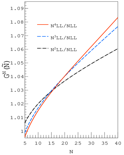
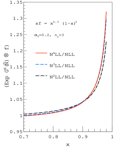
Figure 1: Left: The resummation exponent $G^{N}$, normalized to the NLL results, for DIS in eq. (2.7) plotted successively up to N${}^{4}$LL for $\alpha_{\rm s}=0.2$ and ${n_{\!f}}=3$. Right: The resummed series is convoluted with a typical shape for a quark distribution up to N${}^{4}$LL.

In the left panel of Fig. 1, we present the resummation exponent up to N${}^{4}$LL, normalized to the NLL results for a better visibility of the small higher-order effects. Recall that the resummation accuracy is defined by truncating the resummation exponent in eq. (2.7) to a particular order; i.e., the first term $\ln\widetilde{N}g^{(1)}$ defines the LL approximation, the first two terms $\ln\widetilde{N}g^{(1)}+g^{(2)}$ define the NLL accuracy and so on. Using the order-independent value $\alpha_{\rm s}=0.2$ for the strong coupling, we observe a good perturbative convergence up to N${}^{4}$LL level. At the largest $N$-value shown, $N=40$, the exponent increases from LL to NLL by around $66.7\%$, from NLL to NNLL by around $6.0\%$, from NNLL to N${}^{3}$LL by around $1.5\%$ and from N${}^{3}$LL to N${}^{4}$LL by around $0.6\%$. The resummed series thus shows a good stabilization at this order. The uncertainty in $B_{4}^{\rm DIS}$ quoted in eq. (3.53) as a result of changing the respective large-${n_{c}}$ terms by $\pm 10\%$ does not affect the cross section much. It amounts at most to $0.1\%$, which is small compared to the size of the N${}^{4}$LL correction.

In the right panel of Fig. 1 we plot $\exp(G^{N})\otimes f$, the resummation exponential convoluted with a schematic but sufficiently typical shape for a quark distribution given by $xf=x^{0.5}(1-x)^{3}$. For the Mellin inversion we have used the minimal prescription Catani:1996yz with the standard contour choice as in QCD-Pegasus Vogt:2004ns. Also here we find a good perturbative convergence up to N${}^{4}$LL. At $x=0.9$ the cross section changes from LL to NLL by $67.1\%$, from NLL to NNLL by $4.2\%$, from NNLL to N${}^{3}$LL by $0.09\%$ and from N${}^{3}$LL to N${}^{4}$LL by $-0.17\%$. At $x=0.95$ the corresponding changes are much larger, yet the N${}^{4}$LL effect stays well within $0.5\%$.

For ${n_{\!f}}=4$ light quark flavours on the other hand, we see an even faster perturbative convergence for the resummation exponent as well as for the convolution of exponential with the same input shape. For example, at $N=40$ we observe a $61.4\%$ increase from LL to NLL, another increase of $1.8\%$ from NLL to NNLL, and changes of $-1.1\%$ from NNLL to N${}^{3}$LL and of $-0.9\%$ from N${}^{3}$LL to N${}^{4}$LL accuracy. For the case of the convolution of the exponential with the above input shape, the corresponding values read $61\%,0.3\%,-1.7\%$ and $-0.8\%$, respectively, at $x=0.9$.

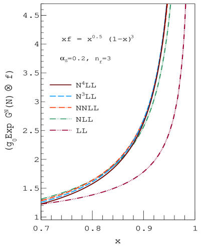
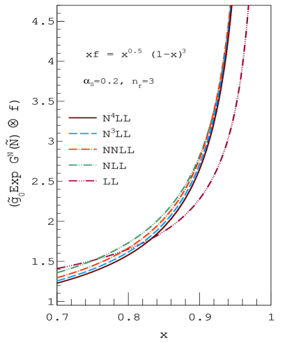
Figure 2: Comparison between the $N$-exponentiation (left) and $\widetilde{N}$-exponentiation (right) as discussed in the text.

The threshold limit in the Mellin-$N$ space is based on the large-$N$ limit, which we have discussed so far in terms of the variable $\widetilde{N}=N\exp(\gamma_{E})$, including the exponentiation of all $\ln\widetilde{N}$ terms. One can, in principle, define the large Mellin variable as $N$ only and collect only those terms in the resummed exponent which are enhanced as $N\to\infty$. As far as the threshold limit is concerned, both, $\widetilde{N}\to\infty$ and $N\to\infty$ are physically equivalent. However, numerically the two options differ since in the former case all $\gamma_{E}$ terms associated with $N$ are also exponentiated to all orders. Due to this feature the results for both cases are different starting already at LL accuracy. The resummed exponent shows a faster convergence for the $N$ exponentiation. However, note that now also the function $g_{0}$ in eq. (2.1) differs between the two cases. Whereas in the $\widetilde{N}$ exponentiation, the $\gamma_{E}$ terms are collected by definition in $\widetilde{N}$ as the large-$N$ variable, for the $N$-exponentiation they are appear in the finite function $g_{0}$ and in the resummed exponent $G$. As mentioned already, we collect the explicit results for the perturbative expansion of $g_{0}$ in the Appendix B.

A useful comparison for these two approaches is therefore to check the convergence at the cross-section level itself. We provide this comparison in Fig. 2. For the $N$-exponentiation satisfactory convergence occurs in the threshold region only beyond NLL accuracy whereas the $\widetilde{N}$-exponentiation shows a systematic behaviour for perturbative convergence for the successive orders of the resummation and good convergence in the threshold region is achieved already at NLL accuracy. At sufficiently high logarithmic order both approaches converge. However they start to differ away from the threshold. At $x=0.7$, the LL result in $\widetilde{N}$-exponentiation differs by as large as $15\%$ compared to the $N$-exponentiation, whereas at the N${}^{4}$LL level this difference decreases to $0.1\%$ showing that at higher logarithmic accuracy they tend to converge. We see similar observation in the higher $x$ region as well. In the rest of the article, we apply the standard $\widetilde{N}$ exponentiation throughout.

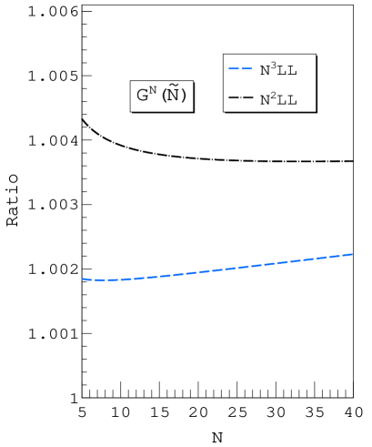
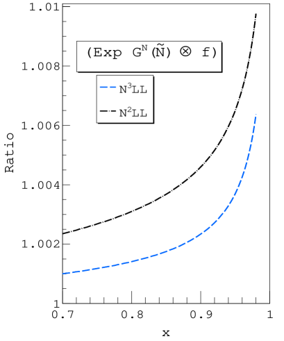
Figure 3: The ratio of large-${n_{c}}$ approximation and the exact results at NNLL and N${}^{3}$LL for $\alpha_{S}=0.2$ and ${n_{\!f}}=3$ light flavours. Left: The ratio for DIS resummed exponent $G^{N}$ as a function of Mellin-$N$. Right: The ratio for the resummed series convoluted with the typical input shape used in Fig. 1 plotted against $x$.

It is instructive to study the quality of the specific large-${n_{c}}$ approximation used to derive the approximate value for $B_{4}^{\rm DIS}$ in eq. (3.53) at each lower order. To that end, we have compared the large-${n_{c}}$ behaviour of results at lower loops with the exact full-colour expressions available up to three loops. Note that in order to have a meaningful estimate of the resummed coefficient function, we take the large-${n_{c}}$ approximation only for the process-dependent pieces appearing at that order, whereas all the lower order terms are kept exact. For example, at the third order, we take the large-${n_{c}}$ approximation only for the combination $-(f_{3}^{\rm q}+B_{3}^{\rm q})$ appearing in eq. (3.46) whereas all the other terms proportional to coefficients of the QCD beta function are kept exact. The LL result is always exact since it only depends on the universal cusp anomalous dimension $A_{1}$ while the first process-dependent coefficients enter as $-(f_{1}^{\rm q}+B_{1}^{\rm q})$ at NLL order. Note that up to the third order the large-$n_{c}$ limit for the terms proportional to ${n^{\,1}_{\!f}}$ and ${n^{\,0}_{\!f}}$ in $f_{i}^{\rm q}$ and $B_{i}^{\rm q}$ coincides with the exact large-$n_{c}$ expressions of these coefficients when restoring the overall factor ${C_{F}}$. However this is not true anymore at the N${}^{4}$LO level.

In Fig. 3, we compare the large-${n_{c}}$ and the exact results for the resummation exponent (left) and the resummed series convoluted with the same quark distribution $xf$ used above (right). In particular we have taken the ratio between the large-${n_{c}}$ and exact results at lower orders. We have taken ${n_{\!f}}=3$ light quark flavours also for this study. Up to NLL the large-${n_{c}}$ result is exact. The difference in the cross section starts from NNLL and is about $0.4\%$ in the large-$N$ region ($N=40$), whereas at N${}^{3}$LL it is about $0.2\%$; the large-${n_{c}}$ approximation always overestimates the exact result in the region of interest. These differences are to be compared with the absolute size of the exact corrections. These are much larger with about $6.0\%$ at $N=40$, when increasing the logarithmic accuracy from NLL to NNLL, and $1.5\%$ for NNLL to N${}^{3}$LL. Similar observations also hold at lower $N$ values.

Using the approximate value for $B_{4}^{\rm DIS}$ in eq. (3.53) with the specific large-${n_{c}}$ limit, the step from N${}^{3}$LL to N${}^{4}$LL accuracy amounts to a correction of about $0.6\%$ at $N=40$. Based on the lower order studies, we thus expect that the exact result at fourth order for the complete N${}^{4}$LL calculation should not differ by more that $\pm 0.2\%$ from our prediction for the resummed exponent at large-${n_{c}}$. In summary, the above procedure of taking the specific large-${n_{c}}$ approximation provides robust estimates for the cross sections of interest.

4.2 Soft-virtual cross section at the fourth order

The convergence of the threshold expansion in Bjorken-$x$ or Mellin-$N$ space can be illustrated by means of the successive addition of the plus-distributions ${\cal D}_{k}$, $k=2n-1,\dots,0$ in the SV cross section in $x$-space compared to the successive addition of the logarithms $\ln^{i}N$, $i=2n,\dots,1$ in $N$-space. The former procedure shows poor convergence, a fact that has been already observed in Catani:1996yz for two ($n=2$) and in Moch:2005ba for three ($n=3$) loops. In Fig. 4 we compare the convergence of the DIS Wilson coefficient at four loops $c^{(4)}_{2,{\rm q}}$ constructed in this manner either in $x$- or in $N$-space and convoluted with the above input shape $xf$. As expected we see a very similar behaviour compared to the known lower orders. The $x$-space result converges poorly and only stabilizes after the addition of the six highest plus-distributions ${\cal D}_{k}$ at this order. On the other hand in $N$-space, the same convergence is achieved much faster after adding only the four highest logarithms $\ln^{i}N$ in the series. This confirms that $N$-space is better suited for studies of the threshold limit also at the fourth order.

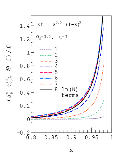
Figure 4: Left: The DIS Wilson coefficient $c^{(4)}_{2,{\rm q}}$ in eq. (3.42) convoluted with the input shape $xf$ of Fig. 1 with the successive addition of the plus-distributions ${\cal D}_{k}$ starting from the highest term. Right: The same with the successive addition of the $N$-space logarithms.

The exact expression of ${\cal D}_{0}$ at fourth order still contains the poorly constrained coefficients $f_{4,\,d^{\,(4)}_{F\!A}}^{\rm q}$, $f_{4,\,{{n_{\!f}}\*{C^{\,3}_{F}}}}^{\rm q}$ and $f_{4,\,{{n_{\!f}}\*{C^{\,2}_{F}}\*{C_{\!A}}}}^{\rm q}$ in eq. (3.2) which drop out in the large-${n_{c}}$ limit. We have improved the ${\cal D}_{0}$ coefficient in eq. (3.43) through the best estimate for $B_{4}^{\rm DIS}$ in eq. (3.53). Using instead the central value for the above $f_{4}$ coefficients (see eq. (3.2)) the ${\cal D}_{0}$ coefficient changes by around $6.5\%$ compared to the value in eq. (3.43). This is a rather small change considering the errors in these coefficients in eq. (3.2). On the other hand setting the $f_{4}$ coefficients in eq. (3.2) to zero, which is within the uncertainty range quoted, yields a value for the ${\cal D}_{0}$ coefficient which differs only by $0.5\%$ from its best prediction in eq. (3.43). These are small effects given that the best estimate for ${\cal D}_{0}$ in eq. (3.43) changes the whole N${}^{4}$LO SV cross-section (up to the contribution proportional to $\delta(1-x)$ in eq. (A)) by only $0.9\%$ even at $x=0.95$. Altogether, this demonstrates a small dependence of the total cross section on those, as of yet, still poorly known coefficients. At the same time, it corroborates the assumptions made in the derivation of the best estimate for ${\cal D}_{0}$ in eq. (3.43).

4.3 Tower expansion vs exponentiation

The resummed cross section in Mellin $N$-space can also be reorganized in a different manner Vogt:1999xa; Moch:2005ba by re-expanding the exponential in eq. (2.1) as follows:

$$C_{a,q}^{\,N}(Q^{2})=1+\sum_{k=1}^{\infty}a_{s}^{k}\sum_{l=1}^{2k}c_{kl}\ln^{2k-l+1}N\,,$$ (4.55)

where the coefficients $c_{kl}$ for DIS are given in Tab. 2 for all known terms. By successive addition of terms in this expansion, one can also predict the resummed cross section up to a certain accuracy. The truncation of this series at any particular order will, of course, recover the fixed-order SV result in $N$-space. The coefficients $c_{kl}$ of the logarithms in the above series vanish factorially at sufficiently higher orders in $\alpha_{\rm s}$ for a fixed logarithmic structure (i.e., fixed by $l$). The coefficients $c_{kl}$ are determined up to $l=1,2,3$ by the complete one loop calculation with NLL resummation. The complete two-loop calculation along with the NNLL resummation fixes the next two towers ($l=4,5$), whereas the complete three-loop calculation along with the N${}^{3}$LL resummation determines again the next two towers, i.e., up to $l=7$. The N${}^{4}$LL resummation derived here allows to completely fix the eighth tower, which corresponds to $l=8$. Note that the quartic colour factors, i.e., $d^{\,(4)}_{F\!A}$ and $d^{\,(4)}_{F\!F}$ in eq. (3.12), appear in this tower for the first time. To obtain all terms up to the ninth tower ($l=9$), the complete four-loop calculation is needed, which is currently not available. However from the knowledge of higher moments for DIS, we can estimate approximate values for the unknown $\delta(1-x)$ coefficient (see Appendix A) at the four loops which in turn can be used to extract the coefficient $g_{04}^{\rm DIS}$. For the standard $\widetilde{N}$ exponentiation, then one can have at the fourth order,

$$g_{04}^{\rm DIS} = (-22.51\pm 3.)\cdot 10^{4}\,,$$ (4.56)

$$(-13.75\pm 3.)\cdot 10^{4}\,,$$

$$(-\phantom{0}6.88\pm 3.)\cdot 10^{4}\,\qquad\text{ for $n_{f}=3,4,5$, respectively.}$$

With the lower orders coefficient the series for $g_{0}$ looks as follows

$$g_{0}(n_{f}=3) =1-16.3865~{}a_{s}-147.955~{}a_{s}^{2}-4528.85~{}a_{s}^{3}-(22.51\pm 3)\cdot 10^{4}~{}a_{s}^{4}$$

$$g_{0}(n_{f}=4) =1-16.3865~{}a_{s}-109.603~{}a_{s}^{2}-2918.08~{}a_{s}^{3}-(13.75\pm 3)\cdot 10^{4}~{}a_{s}^{4}$$

$$g_{0}(n_{f}=5) =1-16.3865~{}a_{s}-71.2505~{}a_{s}^{2}-1477.81~{}a_{s}^{3}-(6.88\pm 3)\cdot 10^{4}~{}a_{s}^{4}\,.$$ (4.57)

The error in the $g_{04}^{\rm DIS}$ coefficient introduces an uncertainty of around $6\%$ in the $\ln^{2}N$ term of the $a_{s}^{5}$ coefficient. The uncertainty in column $c_{k8}$ is due to only the uncertainty coming from the estimate for $B_{4}^{\rm DIS}$. On the other hand the uncertainty due to both $B_{4}^{\rm DIS}$ and $g_{04}^{\rm DIS}$ are added in quadrature to get the final uncertainty in column $c_{k9}$. Although we note that this uncertainty is mostly dominated by the uncertainty in $g_{04}^{\rm DIS}$ estimate. [table]font=tiny

$k$	$c_{k1}$	$c_{k2}$	$c_{k3}$	$c_{k4}$	$c_{k5}$	$c_{k6}$	$c_{k7}$	$c_{k8}$ $(\times 10^{-3})$	$c_{k9}$ $(\times 10^{-4})$
1	2.66667	7.0785	-	-	-	-	-	-	-
2	3.55556	26.8760	46.082	-52.31	-	-	-	-	-
3	3.16049	46.5013	262.409	606.02	-379.3	-1607	-	-	-
4	2.10700	50.8159	526.224	2901.29	7563.9	3839	-30240	-50.45 $\pm$ 1.1	-
5	1.12373	40.1983	643.688	5931.23	32776.2	102186	111002	-223.83 $\pm$ 2.8	-135.79 $\pm$ 8.5
6	0.49944	24.8103	562.907	7611.78	66550.1	380864	1341323	2326.76 $\pm$ 3.8	-136.09 $\pm$ 13.4
7	0.19026	12.5251	381.022	7043.11	87178.2	749259	4455641	17525.89 $\pm$ 3.4	3930.14 $\pm$ 15.2
8	0.06342	5.3423	209.584	5057.26	83343.1	983401	8443647	52347.85 $\pm$ 2.2	22576.03 $\pm$ 13.2
9	0.01879	1.9710	96.844	2951.41	62206.6	956176	10993901	95211.30 $\pm$ 1.2	61509.98 $\pm$ 9.0
10	0.00501	0.6404	38.511	1445.50	37852.3	731699	10762856	122209.70 $\pm$ 0.5	107329.05 $\pm$ 5.0
11	0.00121	0.1858	13.424	608.30	19356.2	458590	8364106	119639.50 $\pm$ 0.2	135303.85 $\pm$ 2.4
12	0.00027	0.0487	4.161	223.97	8508.0	242196	5352115	93780.42 $\pm$ 0.1	131835.19 $\pm$ 1.0
13	0.00006	0.0116	1.161	73.19	3271.3	110118	2895802	60869.59 $\pm$ 0	103720.30 $\pm$ 0.3
14	0.00001	0.0026	0.294	21.48	1115.7	43830	1351835	33532.90 $\pm$ 0	67950.87 $\pm$ 0.1
15	0.00000	0.0005	0.068	5.72	341.4	15479	553238	15980.28 $\pm$ 0	37933.17 $\pm$ 0

Table 2: The coefficients of the tower expansion for $C^{\,N}(Q^{2})$ in eq. (4.55) for ${n_{\!f}}=3$ light quark flavours, where they are the same for $F_{1}$, $F_{2}$ and $F_{3}$ since $fl_{11}=0$. The first seven columns are exact up to the numerical truncation. The eighth column uses the estimates for $B_{4}^{\rm DIS}$ and corresponding errors and the ninth column in addition requires the estimate for $g_{04}^{\rm DIS}$ in eq. (4.56).

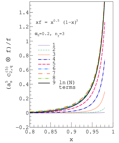
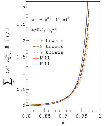
Figure 5: Left: The successive approximations of the five-loop coefficient function $c^{(5)}_{2,{\rm q}}$ by the large-$N$ terms specified in Tab. 2, illustrated by the convolution with the input shape $xf$ of Fig. 1. Right: The corresponding results for the effect of higher terms beyond $\alpha_{\rm s}^{4}$ as obtained from the tower expansion up to nine towers and from the exponentiation up to N${}^{4}$LL accuracy on the Wilson coefficient.

In Fig. 5 on the left we illustrate the expansion in decreasing powers of $\ln\,N$ for the five-loop coefficient function $c^{(5)}_{2,{\rm q}}$ in the same manner as for the four-loop coefficient function $c^{(4)}_{2,{\rm q}}$ in the right part of Fig. 4 above. We confirm the general pattern, that the first $l$ logarithms provide a good estimate up to the $l$-th order in $\alpha_{\rm s}$, i.e., $l=5$ for the case at hand. In the right panel of Fig. 5 we compare the resummed result (exponentiated) for the Wilson coefficient with the tower expansion given in Tab. 2. Although they both converge in the region of $x\simeq 0.5$, they start to diverge at large $x$ where exponentiation shows a better stability compared to the tower expansion. In fact the expansion with a fixed number of towers severely underestimates the effect of the coefficient functions of much higher orders, which become more important at the region of very large-$x$ around $x\simeq 0.9$.

So far we have considered $fl_{11}=0$ for the flavour structure, which holds for ${n_{\!f}}=3$, due to the vanishing combination of the quark charges. Starting from three loops, the neutral-current DIS coefficient functions differ due to $fl_{11}\neq 0$, which captures the effect of incoming and outgoing photons coupling to quark lines of different flavour, see e.g., Vermaseren:2005qc. The effect of this contribution is numerically insignificant as already pointed out in Moch:2005ba. To estimate its numerical impact on the SV cross section as well as in the tower expansion, we use ${n_{\!f}}=4$ and keep the exact value $fl_{11}=1/10$. Note that a non-zero $fl_{11}$ will change the tower expansion starting from seventh tower, i.e., the coefficients $c_{k7}$, and from the lowest order for this towers ($k=3$). In the seventh tower, the contribution proportional to $fl_{11}$ changes the finite piece of third order SV result, whereas at the fourth order in addition it also changes the eight tower. Keeping exact value for $fl_{11}$ we get a difference of $0.1\%$ in the coefficient of the constant term at third order and a change of $0.09\%$ in the last logarithmic term at fourth order.

The additional new term in the charged-current DIS coefficient function $C_{3,q}$ proportional to the group invariant $(d^{\,abc}d_{\,abc})/{n_{c}}$ in eq. (3.10) which corresponds to incoming and outgoing $W^{\pm}$-bosons coupling to a closed internal quark loop Moch:2008fj. This term is power suppressed for $x~{}\to~{}1$, hence does not contribute to the threshold approximation considered here.

5 Summary

We have applied recent progress in the calculation of the cusp anomalous dimension, the quark (non-singlet) splitting functions and the quark form factor to obtain predictions for the DIS cross sections with charged- and neutral-current interactions at four loops in perturbation theory. We have performed the threshold resummation in the large-${n_{c}}$ limit up to N${}^{4}$LL collecting the terms $\alpha_{\rm s}^{\,3}(\alpha_{\rm s}\ln N)^{k}$ to all orders in $\alpha_{\rm s}$ in the threshold resummation exponent $G^{N}$ in Mellin-$N$ space. To that end, the relevant quantity $B^{\rm DIS}$ controlling the resummation of the quark jet function has been extracted at four-loop order.

We have also derived the full colour dependence of the DIS Wilson coefficients at four loops down to the term proportional to the plus-distribution $[1/(1-x)]_{+}$ using a conjecture about the colour structure of the anomalous dimension of the eikonal form factor, namely that it exhibits the same generalized maximal non-Abelian property regarding quadratic and quartic Casimir coefficients as the cusp anomalous dimension. As a by-product, also the single pole of QCD form factor in the parameter of dimensional regularization $\varepsilon$ has been determined numerically to good accuracy.

Using the analytical expressions for the resummed DIS Wilson coefficient at the N${}^{4}$LL level, we have shown that the lower order corrections are sizable and that the threshold logarithms at N${}^{4}$LL resummed order amount to corrections well within $1\%$ and improve the perturbative convergence. We have compared the effect of successive plus-distributions in $x$-space as well as the logarithms in $N$-space for the cross section up to the fourth order and we confirm known observations that the convergence of the logarithmic series in $N$-space is much smoother compared to the one in $x$-space. We have also reorganized the resummed series as a tower of logarithms up to the ninth tower. While the tower expansion is useful to study the effect of higher logarithms, it lacks contributions at very large $x$ compared to the exponentiated result. The latter exhibits an even better stability even in the very large-$x$ region. Near threshold the difference between DIS Wilson coefficients for charged- and neutral-current exchange, which manifests itself in the flavour structure $fl_{11}$ at three loops and beyond, has only a minor numerical effect (for ${n_{\!f}}=4$) on the respective cross sections.

The current accuracy can be significantly improved with the knowledge of the complete QCD form factor at four loops or an exact computation of the corresponding eikonal anomalous dimension at this order. In particular analytic results for all ${n_{\!f}}$ dependent terms in those quantities would greatly reduce the present residual numerical uncertainties. At the accuracy reached with N${}^{4}$LL resummation also power corrections proportional to $1/N$ in Mellin-$N$ space or logarithmic enhancement $\ln^{k}(1-x)$ in $x$-space become numerically relevant, see Moch:2009hr; Bonocore:2015esa. Finally, the effects from the massive quarks are important in the threshold region (see for example Kawamura:2012cr; Hoang:2015iva) and a proper treatment of heavy quark mass effects becomes essential for phenomenological applications.

——————————————————————–

Acknowledgments

G.D. thanks V. Ravindran for useful discussions. The algebraic computations have been done with the latest version of the symbolic manipulation system Form Vermaseren:2000nd; Ruijl:2017dtg. This work has been supported by the Deutsche Forschungsgemeinschaft (DFG) under grant number MO 1801/2-1, and by the COST Action CA16201 PARTICLEFACE supported by European Cooperation in Science and Technology (COST). The research of G.D. is supported by the DFG within the Collaborative Research Center TRR 257 (“Particle Physics Phenomenology after the Higgs Discovery”).

Note added in proof

During review of the present paper, the complete analytic four-loop anomalous dimensions in massless QCD from form factors have been obtained in vonManteuffel:2020vjv. This provides information on the missing four-loop contributions $f_{4,\,{{n_{\!f}}\*{C^{\,3}_{F}}}}^{\rm q}$ and $f_{4,\,{{n_{\!f}}\*{C^{\,2}_{F}}\*{C_{\!A}}}}^{\rm q}$ in eq. (3.2), which we can determine as

$$f_{4,\,{{n_{\!f}}\*{C^{\,3}_{F}}}}^{\rm q} = \frac{27949}{108}+322\*\zeta_{2}-\frac{1120}{9}\*\zeta_{3}-334\*\zeta_{4}-\frac{512}{3}\*\zeta_{2}\*\zeta_{3}+\frac{3872}{3}\*\zeta_{5}+368\*\zeta_{3}^{2}$$

$$-\frac{14668}{9}\*\zeta_{6}-2\*b_{4,\,{{n_{\!f}}\*{C^{\,3}_{F}}}}^{\rm q}$$

$$= -9.626\pm 0.010\,,$$

$$f_{4,\,{{n_{\!f}}\*{C^{\,2}_{F}}\*{C_{\!A}}}}^{\rm q} = -\frac{1092511}{972}+\frac{673}{27}\*\zeta_{2}-\frac{23518}{81}\*\zeta_{3}+\frac{52744}{27}\*\zeta_{4}+\frac{3904}{9}\*\zeta_{2}\*\zeta_{3}-\frac{4472}{3}\*\zeta_{5}$$ (5.58)

$$-\frac{3400}{3}\*\zeta_{3}^{2}+718\*\zeta 6-2\*b_{4,\,{{n_{\!f}}\*{C^{\,2}_{F}}\*{C_{\!A}}}}^{\rm q}$$

$$= -2.351\pm 0.010\,.$$

Their numerical values are in agreement with those quoted in eq. (3.2). The remaining uncertainties in eq. (5) are due to the numerical values in Tab. 1. We have verfied that the large-${n_{c}}$ results for ${n_{\!f}}=3$, $4$ or $5$ at four loops in eq. (3.2) reproduce full QCD within ${\cal O}(1\%)$.

This new information in eq. (5) leads to the following numerical result for the coefficient proportional to ${\cal D}_{0}$ in the DIS Wilson coefficients $c^{(4)}_{a,{\rm q}}$ in eq. (3.43),

$$c^{(4)}_{2,{\rm q}}\biggr{|}_{{\cal D}_{0}} = (3.874\pm 0.010)\cdot 10^{4}+(-3.4965\pm 0.0287)\cdot 10^{4}\,\*{n_{\!f}}+2062.715\,\*{n^{\,2}_{\!f}}$$ (5.59)

$$\mbox{}-12.08488\,\*{n^{\,3}_{\!f}}+47.55183\,\*{n_{\!f}}\*fl_{11}\>\>,$$

where all exact values have been rounded to seven digits. The remaining errors come either from the uncertainty for $f_{4,\,d^{\,(4)}_{F\!A}}^{\rm q}$ in eq. (3.2) (term proportional to ${n^{\,0}_{\!f}}$) or from the numerical values in Tab. 1 (term proportional to ${n^{\,1}_{\!f}}$). The new numerical value in eq. (5.59) agrees very well with the best estimate in eq. (3.43). This also corroborates the arguments based on the large-${n_{c}}$ limit.

With the full colour dependence in eq. (5.59) at hand, the resummation coefficient $B_{4}^{\rm DIS}$ in eq. (3.52) then becomes

$$B_{4}^{\rm DIS} = (10.68\pm 0.01)\cdot 10^{4}+(-2.0275549\pm 0.0000029)\cdot 10^{4}\,\*{n_{\!f}}+798.0698\,\*{n^{\,2}_{\!f}}$$ (5.60)

$$\qquad-12.08488\,\*{n^{\,3}_{\!f}}\,,$$

where the uncertainty in the term proportional to ${n^{\,1}_{\!f}}$ stems from the numerical values in Tab. 1. Again, this agrees very well with the previous best estimate in eq. (3.53) based on the large-${n_{c}}$ limit. The perturbative expansion of $B^{\rm DIS}$ through four loops (replacing eq. (3.4)) reads then

$$B^{\rm DIS}({n_{\!f}}\!=\!3) = -0.31831\,\alpha_{\rm s}\>(1-1.1004\,\alpha_{\rm s}-3.623\,\alpha_{\rm s}^{2}-(6.659\pm 0.013)\,\alpha_{\rm s}^{3}+\,\ldots)\;,$$

$$B^{\rm DIS}({n_{\!f}}\!=\!4) = -0.31831\,\alpha_{\rm s}\>(1-1.2267\,\alpha_{\rm s}-3.405\,\alpha_{\rm s}^{2}-(4.753\pm 0.013)\,\alpha_{\rm s}^{3}+\,\ldots)\;,$$

$$B^{\rm DIS}({n_{\!f}}\!=\!5) = -0.31831\,\alpha_{\rm s}\>(1-1.3530\,\alpha_{\rm s}-3.190\,\alpha_{\rm s}^{2}-(3.010\pm 0.013)\,\alpha_{\rm s}^{3}+\,\ldots)\,,$$

(5.61)

which eliminates any residual uncertainty in the resummation at N${}^{4}$LL accuracy.

Appendix A DIS Wilson coefficients

For convenience of the reader we have collected all available information on the soft-virtual expressions for the DIS coefficient functions $c^{(n)}_{2,{\rm q}}$ through four loops $(n\leq 4)$. The leading order is $c^{(0)}_{2,{\rm q}}=\delta(1-x)$ and the one-loop result $c^{(1)}_{2,{\rm q}}$ in eq. (A.1) has been obtained in Bardeen:1978yd. The two- and three-loop expressions $c^{(2)}_{2,{\rm q}}$ and $c^{(3)}_{2,{\rm q}}$ in eqs. (A.2), (A.3) are due to vanNeerven:1991nn; Moch:1999eb and Vermaseren:2005qc, respectively. At four loops all plus-distributions ${\cal D}_{\,k}$ with $k\geq 2$ in $c^{(4)}_{2,{\rm q}}$ have been given in Moch:2005ba. The terms ${\cal D}_{\,1}$ with the complete colour dependence of $A_{4}$ inserted and ${\cal D}_{\,0}$ in $c^{(4)}_{2,{\rm q}}$ are new results. Analytical results for the coefficients $f_{4,\,{{n_{\!f}}\*{C^{\,3}_{F}}}}^{\rm q}$, $f_{4,\,{{n_{\!f}}\*{C^{\,2}_{F}}\*{C_{\!A}}}}^{\rm q}$ and $f_{4,\,d^{\,(4)}_{F\!A}}^{\rm q}$ can be expected from the computation of the form factor at four loops soon. The remaining coefficients $b_{4,\,{{C^{\,4}_{F}}}}^{\rm q}$, $b_{4,\,{{C^{\,3}_{F}}\*{C_{\!A}}}}^{\rm q}$, $b_{4,\,{{C^{\,2}_{F}}\*{C^{\,2}_{\!A}}}}^{\rm q}$, $b_{4,\,{{n_{\!f}}\*{C^{\,3}_{F}}}}^{\rm q}$, $b_{4,\,{{n_{\!f}}\*{C^{\,2}_{F}}\*{C_{\!A}}}}^{\rm q}$, $b_{4,\,d^{\,(4)}_{F\!A}}^{\rm q}$, and $b_{4,\,d^{\,(4)}_{F\!F}}^{\rm q}$ of the virtual anomalous dimension $B_{4}^{\rm q}$ require an analytical result for the four-loop splitting function, which is not easily available. The factors $fl_{11}$ in eqs. (A.3), (A.4) do not appear in charged-current DIS.

$$c^{(1)}_{2,{\rm q}} = 4\*{C_{F}}\*{\cal D}_{1}-3\*{C_{F}}\*{\cal D}_{0}-{C_{F}}\*(9+4\*\zeta_{2})\*\delta(1-x)\,,$$ (A.1)

$$c^{(2)}_{2,{\rm q}} = 8\*{C^{\,2}_{F}}\*{\cal D}_{3}-{\cal D}_{2}\*\biggl{\{}18\*{C^{\,2}_{F}}+\frac{22}{3}\*{C_{F}}\*{C_{\!A}}-\frac{4}{3}\*{C_{F}}\*{n_{\!f}}\biggr{\}}+{\cal D}_{1}\*\biggl{\{}-{C^{\,2}_{F}}\*(27+32\*\zeta_{2})$$ (A.2)

$$+{C_{F}}\*{C_{\!A}}\*\biggl{(}\frac{367}{9}-8\*\zeta_{2}\biggr{)}-\frac{58}{9}\*{C_{F}}\*{n_{\!f}}\biggr{\}}+{\cal D}_{0}\*\biggl{\{}{C^{\,2}_{F}}\*\biggl{(}\frac{51}{2}+36\*\zeta_{2}-8\*\zeta_{3}\biggr{)}$$

$$-{C_{F}}\*{C_{\!A}}\*\biggl{(}\frac{3155}{54}-\frac{44}{3}\*\zeta_{2}-40\*\zeta_{3}\biggr{)}+{C_{F}}\*{n_{\!f}}\*\biggl{(}\frac{247}{27}-\frac{8}{3}\*\zeta_{2}\biggr{)}\biggr{\}}+\delta(1-x)\*\biggl{\{}{C^{\,2}_{F}}\*\biggl{(}\frac{331}{8}$$

$$+69\*\zeta_{2}-78\*\zeta_{3}+6\*\zeta_{2}^{\,2}\biggr{)}-{C_{F}}\*{C_{\!A}}\*\biggl{(}\frac{5465}{72}+\frac{251}{3}\*\zeta_{2}-\frac{140}{3}\*\zeta_{3}-\frac{71}{5}\*\zeta_{2}^{\,2}\biggr{)}$$

$$+{C_{F}}\*{n_{\!f}}\*\biggl{(}\frac{457}{36}+\frac{38}{3}\*\zeta_{2}+\frac{4}{3}\*\zeta_{3}\biggr{)}\biggr{\}}\,,$$

$$c^{(3)}_{2,{\rm q}} = 8\*{C^{\,3}_{F}}\*{\cal D}_{5}+{\cal D}_{4}\*\biggl{\{}-30\*{C^{\,3}_{F}}-\frac{220}{9}\*{C^{\,2}_{F}}\*{C_{\!A}}+\frac{40}{9}\*{C^{\,2}_{F}}\*{n_{\!f}}\ \biggr{\}}+{\cal D}_{3}\*\biggl{\{}-{C^{\,3}_{F}}\*(36+96\*\zeta_{2})$$ (A.3)

$$+{C^{\,2}_{F}}\*{C_{\!A}}\*\biggl{(}\frac{1732}{9}-32\*\zeta_{2}\biggr{)}+\frac{484}{27}\*{C_{F}}\*{C^{\,2}_{\!A}}-\frac{280}{9}\*{C^{\,2}_{F}}\*{n_{\!f}}-\frac{176}{27}\*{C_{F}}\*{C_{\!A}}\*{n_{\!f}}+\frac{16}{27}\*{C_{F}}\*{n^{\,2}_{\!f}}\biggr{\}}$$

$$+{\cal D}_{2}\*\biggl{\{}{C^{\,3}_{F}}\*\biggl{(}\frac{279}{2}+288\*\zeta_{2}+16\*\zeta_{3}\biggr{)}-{C^{\,2}_{F}}\*{C_{\!A}}\*\biggl{(}\frac{8425}{18}-\frac{724}{3}\*\zeta_{2}-240\*\zeta_{3}\biggr{)}$$

$$-{C_{F}}\*{C^{\,2}_{\!A}}\*\biggl{(}\frac{4649}{27}-\frac{88}{3}\*\zeta_{2}\biggr{)}+{C^{\,2}_{F}}\*{n_{\!f}}\*\biggl{(}\frac{683}{9}-\frac{112}{3}\*\zeta_{2}\biggr{)}+{C_{F}}\*{C_{\!A}}\*{n_{\!f}}\*\biggl{(}\frac{1552}{27}-\frac{16}{3}\*\zeta_{2}\biggr{)}$$

$$-\frac{116}{27}\*{C_{F}}\*{n^{\,2}_{\!f}}\biggr{\}}+{\cal D}_{1}\*\biggl{\{}{C^{\,3}_{F}}\*\biggl{(}\frac{187}{2}+240\*\zeta_{2}-360\*\zeta_{3}+\frac{376}{5}\*\zeta_{2}^{\,2}\biggr{)}-{C^{\,2}_{F}}\*{C_{\!A}}\*\biggl{(}\frac{5563}{18}$$

$$+972\*\zeta_{2}+\frac{160}{3}\*\zeta_{3}-\frac{764}{5}\*\zeta_{2}^{\,2}\biggr{)}+{C_{F}}\*{C^{\,2}_{\!A}}\*\biggl{(}\frac{50689}{81}-\frac{680}{3}\*\zeta_{2}-264\*\zeta_{3}+\frac{176}{5}\*\zeta_{2}^{\,2}\biggr{)}$$

$$+{C^{\,2}_{F}}\*{n_{\!f}}\*\biggl{(}\frac{83}{9}+168\*\zeta_{2}+\frac{112}{3}\*\zeta_{3}\biggr{)}-{C_{F}}\*{C_{\!A}}\*{n_{\!f}}\*\biggl{(}\frac{15062}{81}-\frac{512}{9}\*\zeta_{2}-16\*\zeta_{3}\biggr{)}$$

$$+{C_{F}}\*{n^{\,2}_{\!f}}\*\biggl{(}\frac{940}{81}-\frac{32}{9}\*\zeta_{2}\biggr{)}\biggr{\}}+{\cal D}_{0}\*\biggl{\{}-{C^{\,3}_{F}}\*\biggl{(}\frac{1001}{8}+429\*\zeta_{2}-274\*\zeta_{3}+210\*\zeta_{2}^{\,2}-32\*\zeta_{2}\*\zeta_{3}$$

$$-432\*\zeta_{5}\biggr{)}+{C^{\,2}_{F}}\*{C_{\!A}}\*\biggl{(}\frac{16981}{24}+\frac{26885}{27}\*\zeta_{2}-\frac{3304}{9}\*\zeta_{3}-209\*\zeta_{2}^{\,2}-400\*\zeta_{2}\*\zeta_{3}-120\*\zeta_{5}\biggr{)}$$

$$-{C_{F}}\*{C^{\,2}_{\!A}}\*\biggl{(}\frac{599375}{729}-\frac{32126}{81}\*\zeta_{2}-\frac{21032}{27}\*\zeta_{3}+\frac{652}{15}\*\zeta_{2}^{\,2}+\frac{176}{3}\*\zeta_{2}\*\zeta_{3}+232\*\zeta_{5}\biggr{)}$$

$$-{C^{\,2}_{F}}\*{n_{\!f}}\*\biggl{(}\frac{2003}{108}+\frac{4226}{27}\*\zeta_{2}+60\*\zeta_{3}-16\*\zeta_{2}^{\,2}\biggr{)}+{C_{F}}\*{C_{\!A}}\*{n_{\!f}}\*\biggl{(}\frac{160906}{729}-\frac{776}{9}\*\zeta_{3}-\frac{9920}{81}\*\zeta_{2}$$

$$+\frac{208}{15}\*\zeta_{2}^{\,2}\biggr{)}-{C_{F}}\*{n^{\,2}_{\!f}}\*\biggl{(}\frac{8714}{729}-\frac{232}{27}\*\zeta_{2}+\frac{32}{27}\*\zeta_{3}\biggr{)}\biggr{\}}+\delta(1-x)\*\biggl{\{}-{C^{\,3}_{F}}\*\biggl{(}\frac{7255}{24}+\frac{3379}{6}\*\zeta_{2}$$

$$+318\*\zeta_{3}+\frac{2148}{5}\*\zeta_{2}^{\,2}-808\*\zeta_{2}\*\zeta_{3}-1240\*\zeta_{5}+\frac{304}{3}\*{\zeta_{3}^{\,2}}-\frac{4184}{315}\*{\zeta_{2}^{\,3}}\biggr{)}+{C^{\,2}_{F}}\*{C_{\!A}}\*\biggl{(}\frac{9161}{12}$$

$$+\frac{104117}{54}\*\zeta_{2}-\frac{6419}{3}\*\zeta_{3}+\frac{87632}{135}\*\zeta_{2}^{\,2}-\frac{6644}{9}\*\zeta_{2}\*\zeta_{3}-\frac{4952}{9}\*\zeta_{5}+\frac{1016}{3}\*{\zeta_{3}^{\,2}}-\frac{33556}{315}\*{\zeta_{2}^{\,3}}\biggr{)}$$

$$-{C_{F}}\*{C^{\,2}_{\!A}}\*\biggl{(}\frac{1909753}{1944}+\frac{143255}{81}\*\zeta_{2}-\frac{105712}{81}\*\zeta_{3}-\frac{25184}{135}\*\zeta_{2}^{\,2}-540\*\zeta_{2}\*\zeta_{3}+\frac{416}{3}\*\zeta_{5}$$

$$+\frac{248}{3}\*{\zeta_{3}^{\,2}}+\frac{3512}{63}\*{\zeta_{2}^{\,3}}\biggr{)}-{C^{\,2}_{F}}\*{n_{\!f}}\*\biggl{(}\frac{341}{36}+\frac{5491}{27}\*\zeta_{2}-\frac{1348}{3}\*\zeta_{3}+\frac{16472}{135}\*\zeta_{2}^{\,2}+\frac{352}{9}\*\zeta_{2}\*\zeta_{3}$$

$$+\frac{592}{9}\*\zeta_{5}\biggr{)}+{C_{F}}\*{C_{\!A}}\*{n_{\!f}}\*\biggl{(}\frac{142883}{486}+\frac{40862}{81}\*\zeta_{2}-\frac{18314}{81}\*\zeta_{3}-\frac{2488}{135}\*\zeta_{2}^{\,2}-\frac{56}{3}\*\zeta_{2}\*\zeta_{3}+\frac{8}{3}\*\zeta_{5}\biggr{)}$$

$$-{C_{F}}\*{n^{\,2}_{\!f}}\*\biggl{(}\frac{9517}{486}+\frac{860}{27}\*\zeta_{2}+\frac{152}{81}\*\zeta_{3}+\frac{32}{27}\*\zeta_{2}^{\,2}\biggr{)}+fl_{11}\*{n_{\!f}}\*{{d^{abc}d_{abc}}\over{n_{c}}}\*\biggl{(}64+160\*\zeta_{2}+\frac{224}{3}\*\zeta_{3}$$

$$-\frac{32}{5}\*\zeta_{2}^{\,2}-\frac{1280}{3}\*\zeta_{5}\biggr{)}\biggr{\}}\,,$$

$$c^{(4)}_{2,{\rm q}} = \frac{16}{3}\*{C^{\,4}_{F}}\*{\cal D}_{7}+{\cal D}_{6}\*\biggl{\{}-28\*{C^{\,4}_{F}}-\frac{308}{9}\*{C^{\,3}_{F}}\*{C_{\!A}}+\frac{56}{9}\*{C^{\,3}_{F}}\*{n_{\!f}}\biggr{\}}+{\cal D}_{5}\*\biggl{\{}-{C^{\,4}_{F}}\*(18+128\*\zeta_{2})$$ (A.4)

$$+{C^{\,3}_{F}}\*{C_{\!A}}\*\biggl{(}\frac{998}{3}-48\*\zeta_{2}\biggr{)}+\frac{1936}{27}\*{C^{\,2}_{F}}\*{C^{\,2}_{\!A}}-\frac{164}{3}\*{C^{\,3}_{F}}\*{n_{\!f}}-\frac{704}{27}\*{C^{\,2}_{F}}\*{C_{\!A}}\*{n_{\!f}}+\frac{64}{27}\*{C^{\,2}_{F}}\*{n^{\,2}_{\!f}}\biggr{\}}$$

$$+{\cal D}_{4}\*\biggl{\{}{C^{\,4}_{F}}\*\biggl{(}210+600\*\zeta_{2}+\frac{400}{3}\*\zeta_{3}\biggr{)}-{C^{\,3}_{F}}\*{C_{\!A}}\*\biggl{(}\frac{27835}{27}-\frac{6800}{9}\*\zeta_{2}-400\*\zeta_{3}\biggr{)}$$

$$-{C^{\,2}_{F}}\*{C^{\,2}_{\!A}}\*\biggl{(}\frac{24040}{27}-\frac{440}{3}\*\zeta_{2}\biggr{)}-\frac{1331}{27}\*{C_{F}}\*{C^{\,3}_{\!A}}+{C^{\,3}_{F}}\*{n_{\!f}}\*\biggl{(}\frac{4630}{27}-\frac{1040}{9}\*\zeta_{2}\biggr{)}$$

$$+{C^{\,2}_{F}}\*{C_{\!A}}\*{n_{\!f}}\*\biggl{(}\frac{8120}{27}-\frac{80}{3}\*\zeta_{2}\biggr{)}+\frac{242}{9}\*{C_{F}}\*{C^{\,2}_{\!A}}\*{n_{\!f}}-\frac{640}{27}\*{C^{\,2}_{F}}\*{n^{\,2}_{\!f}}-\frac{44}{9}\*{C_{F}}\*{C_{\!A}}\*{n^{\,2}_{\!f}}+\frac{8}{27}\*{C_{F}}\*{n^{\,3}_{\!f}}\biggr{\}}$$

$$+{\cal D}_{3}\*\biggl{\{}{C^{\,4}_{F}}\*\biggl{(}\frac{113}{2}+264\*\zeta_{2}-1072\*\zeta_{3}+\frac{1392}{5}\*\zeta_{2}^{\,2}\biggr{)}-{C^{\,3}_{F}}\*{C_{\!A}}\*\biggl{(}\frac{1534}{3}+\frac{41824}{9}\*\zeta_{2}$$

$$+\frac{8800}{9}\*\zeta_{3}-\frac{3128}{5}\*\zeta_{2}^{\,2}\biggr{)}+{C^{\,2}_{F}}\*{C^{\,2}_{\!A}}\*\biggl{(}\frac{2154563}{486}-\frac{52912}{27}\*\zeta_{2}-\frac{13024}{9}\*\zeta_{3}+\frac{864}{5}\*\zeta_{2}^{\,2}\biggr{)}$$

$$+{C_{F}}\*{C^{\,3}_{\!A}}\*\biggl{(}\frac{55627}{81}-\frac{968}{9}\*\zeta_{2}\biggr{)}-{C^{\,2}_{F}}\*{C_{\!A}}\*{n_{\!f}}\*\biggl{(}\frac{339134}{243}-\frac{14096}{27}\*\zeta_{2}-\frac{1216}{9}\*\zeta_{3}\biggr{)}$$

$$-{C^{\,3}_{F}}\*{n_{\!f}}\*\biggl{(}\frac{280}{3}-\frac{7216}{9}\*\zeta_{2}-\frac{1888}{9}\*\zeta_{3}\biggr{)}-{C_{F}}\*{C^{\,2}_{\!A}}\*{n_{\!f}}\*\biggl{(}\frac{9502}{27}-\frac{352}{9}\*\zeta_{2}\biggr{)}$$

$$+{C^{\,2}_{F}}\*{n^{\,2}_{\!f}}\*\biggl{(}\frac{24238}{243}-\frac{928}{27}\*\zeta_{2}\biggr{)}+{C_{F}}\*{C_{\!A}}\*{n^{\,2}_{\!f}}\*\biggl{(}\frac{1540}{27}-\frac{32}{9}\*\zeta_{2}\biggr{)}-\frac{232}{81}\*{C_{F}}\*{n^{\,3}_{\!f}}\biggr{\}}$$

$$+{\cal D}_{2}\*\biggl{\{}-{C^{\,4}_{F}}\*\biggl{(}\frac{1299}{2}+2808\*\zeta_{2}-1392\*\zeta_{3}+1836\*\zeta_{2}^{\,2}+640\*\zeta_{2}\*\zeta_{3}-4128\*\zeta_{5}\biggr{)}$$

$$+{C^{\,3}_{F}}\*{C_{\!A}}\*\biggl{(}\frac{13990}{3}+\frac{30704}{3}\*\zeta_{2}+\frac{2716}{3}\*\zeta_{3}-\frac{12906}{5}\*\zeta_{2}^{\,2}-3648\*\zeta_{2}\*\zeta_{3}-720\*\zeta_{5}\biggr{)}$$

$$-{C^{\,2}_{F}}\*{C^{\,2}_{\!A}}\*\biggl{(}\frac{2254339}{243}-\frac{86804}{9}\*\zeta_{2}-\frac{24544}{3}\*\zeta_{3}+\frac{4034}{3}\*\zeta_{2}^{\,2}+832\*\zeta_{2}\*\zeta_{3}+1392\*\zeta_{5}\biggr{)}$$

$$-{C_{F}}\*{C^{\,3}_{\!A}}\*\biggl{(}\frac{649589}{162}-\frac{4012}{3}\*\zeta_{2}-1452\*\zeta_{3}+\frac{968}{5}\*\zeta_{2}^{\,2}\biggr{)}-{C^{\,3}_{F}}\*{n_{\!f}}\*\biggl{(}\frac{145}{9}+\frac{5132}{3}\*\zeta_{2}+936\*\zeta_{3}$$

$$-\frac{1032}{5}\*\zeta_{2}^{\,2}\biggr{)}+{C^{\,2}_{F}}\*{C_{\!A}}\*{n_{\!f}}\*\biggl{(}\frac{713162}{243}-\frac{10600}{9}\*\zeta_{3}-\frac{82004}{27}\*\zeta_{2}+\frac{3772}{15}\*\zeta_{2}^{\,2}\biggr{)}$$

$$+{C_{F}}\*{C^{\,2}_{\!A}}\*{n_{\!f}}\*\biggl{(}\frac{17189}{9}-\frac{5096}{9}\*\zeta_{2}-352\*\zeta_{3}+\frac{176}{5}\*\zeta_{2}^{\,2}\biggr{)}-{C^{\,2}_{F}}\*{n^{\,2}_{\!f}}\*\biggl{(}\frac{52678}{243}-\frac{6104}{27}\*\zeta_{2}$$

$$-\frac{304}{9}\*\zeta_{3}\biggr{)}-{C_{F}}\*{C_{\!A}}\*{n^{\,2}_{\!f}}\*\biggl{(}\frac{7403}{27}-\frac{688}{9}\*\zeta_{2}-16\*\zeta_{3}\biggr{)}+{C_{F}}\*{n^{\,3}_{\!f}}\*\biggl{(}\frac{940}{81}-\frac{32}{9}\*\zeta_{2}\biggr{)}\biggr{\}}$$

$$+{\cal D}_{1}\*\biggl{\{}-{C^{\,4}_{F}}\*\biggl{(}\frac{19885}{24}+\frac{3101}{3}\*\zeta_{2}+1374\*\zeta_{3}+1098\*\zeta_{2}^{\,2}-5824\*\zeta_{2}\*\zeta_{3}-64\*\zeta_{5}+\frac{256}{3}\*{\zeta_{3}^{\,2}}$$

$$+\frac{64192}{315}\*{\zeta_{2}^{\,3}}\biggr{)}+{C^{\,3}_{F}}\*{C_{\!A}}\*\biggl{(}\frac{2829}{2}+\frac{202705}{27}\*\zeta_{2}-\frac{333526}{27}\*\zeta_{3}+\frac{1043747}{135}\*\zeta_{2}^{\,2}+\frac{23104}{9}\*\zeta_{2}\*\zeta_{3}$$

$$-\frac{77216}{9}\*\zeta_{5}+\frac{5984}{3}\*{\zeta_{3}^{\,2}}-\frac{55472}{63}\*{\zeta_{2}^{\,3}}\biggr{)}-{C^{\,2}_{F}}\*{C^{\,2}_{\!A}}\*\biggl{(}\frac{21987073}{5832}+\frac{713440}{27}\*\zeta_{2}+\frac{238400}{81}\*\zeta_{3}$$

$$-\frac{812819}{135}\*\zeta_{2}^{\,2}-\frac{24896}{3}\*\zeta_{2}\*\zeta_{3}-\frac{6472}{3}\*\zeta_{5}-\frac{3808}{3}\*{\zeta_{3}^{\,2}}+\frac{51848}{63}\*{\zeta_{2}^{\,3}}\biggr{)}+{C_{F}}\*{C^{\,3}_{\!A}}\*\biggl{(}\frac{16865531}{1458}$$

$$-\frac{156238}{27}\*\zeta_{2}-\frac{78296}{9}\*\zeta_{3}+\frac{17996}{15}\*\zeta_{2}^{\,2}+528\*\zeta_{2}\*\zeta_{3}+\frac{19360}{9}\*\zeta_{5}-16\*{\zeta_{3}^{\,2}}-\frac{20032}{105}\*{\zeta_{2}^{\,3}}\biggr{)}$$

$$+{\frac{d_{F}^{\,abcd}d_{A}^{\,abcd}}{n_{F}}}\*\biggl{(}-128\*\zeta_{2}+\frac{128}{3}\*\zeta_{3}+\frac{3520}{3}\*\zeta_{5}-384\*{\zeta_{3}^{\,2}}-\frac{7936}{35}\*{\zeta_{2}^{\,3}}\biggr{)}$$

$$+{C^{\,3}_{F}}\*{n_{\!f}}\*\biggl{(}\frac{1775}{18}-\frac{7912}{27}\*\zeta_{2}+\frac{78328}{27}\*\zeta_{3}-\frac{195716}{135}\*\zeta_{2}^{\,2}+\frac{6368}{9}\*\zeta_{5}-\frac{6592}{9}\*\zeta_{2}\*\zeta_{3}\biggr{)}$$

$$-{C_{F}}\*{C^{\,2}_{\!A}}\*{n_{\!f}}\*\biggl{(}\frac{2452247}{486}-\frac{68836}{27}\*\zeta_{2}-\frac{5752}{3}\*\zeta_{3}+\frac{3944}{15}\*\zeta_{2}^{\,2}-32\*\zeta_{2}\*\zeta_{3}+\frac{2080}{9}\*\zeta_{5}\biggr{)}$$

$$-{C^{\,2}_{F}}\*{C_{\!A}}\*{n_{\!f}}\*\biggl{(}\frac{326570}{729}-\frac{694654}{81}\*\zeta_{2}-\frac{158740}{81}\*\zeta_{3}+\frac{178642}{135}\*\zeta_{2}^{\,2}+\frac{2848}{3}\*\zeta_{2}\*\zeta_{3}+\frac{208}{3}\*\zeta_{5}\biggr{)}$$

$$+{n_{\!f}}\*{\frac{d_{F}^{\,abcd}d_{F}^{\,abcd}}{n_{F}}}\*\biggl{(}256\*\zeta_{2}-\frac{256}{3}\*\zeta_{3}-\frac{1280}{3}\*\zeta_{5}\biggr{)}+{C^{\,2}_{F}}\*{n^{\,2}_{\!f}}\*\biggl{(}\frac{239633}{1458}-\frac{50140}{81}\*\zeta_{2}-\frac{19304}{81}\*\zeta_{3}$$

$$+\frac{1312}{27}\*\zeta_{2}^{\,2}\biggr{)}+{C_{F}}\*{C_{\!A}}\*{n^{\,2}_{\!f}}\*\biggl{(}\frac{315755}{486}-\frac{9848}{27}\*\zeta_{2}-\frac{688}{9}\*\zeta_{3}+\frac{64}{5}\*\zeta_{2}^{\,2}\biggr{)}-{C_{F}}\*{n^{\,3}_{\!f}}\*\biggl{(}\frac{17716}{729}$$

$$-\frac{464}{27}\*\zeta_{2}\biggr{)}+fl_{11}\*{C_{F}}\*{n_{\!f}}\*{{d^{abc}d_{abc}}\over{n_{c}}}\*\biggl{(}256+640\*\zeta_{2}+\frac{896}{3}\*\zeta_{3}-\frac{128}{5}\*\zeta_{2}^{\,2}-\frac{5120}{3}\*\zeta_{5}\biggr{)}\biggr{\}}$$

$$+{\cal D}_{0}\*\biggl{\{}{C^{\,4}_{F}}\*\biggl{(}\frac{15605}{16}+2803\*\zeta_{2}+1064\*\zeta_{3}+\frac{19839}{5}\*\zeta_{2}^{\,2}-5168\*\zeta_{2}\*\zeta_{3}-6744\*\zeta_{5}+736\*{\zeta_{3}^{\,2}}$$

$$+\frac{17624}{21}\*{\zeta_{2}^{\,3}}-4992\*\zeta_{2}\*\zeta_{5}-\frac{752}{5}\*\zeta_{2}^{\,2}\*\zeta_{3}+3840\*\zeta_{7}-~{}b_{4,\,{{C^{\,4}_{F}}}}^{\rm q}~{}\biggr{)}-{C^{\,3}_{F}}\*{C_{\!A}}\*\biggl{(}\frac{137084}{27}$$

$$+16683\*\zeta_{2}-\frac{27860}{3}\*\zeta_{3}+\frac{1975109}{270}\*\zeta_{2}^{\,2}-\frac{44332}{9}\*\zeta_{2}\*\zeta_{3}-\frac{29240}{3}\*\zeta_{5}+\frac{12008}{3}\*{\zeta_{3}^{\,2}}-\frac{906268}{315}\*{\zeta_{2}^{\,3}}$$

$$+192\*\zeta_{2}\*\zeta_{5}-\frac{7992}{5}\*\zeta_{2}^{\,2}\*\zeta_{3}+~{}b_{4,\,{{C^{\,3}_{F}}\*{C_{\!A}}}}^{\rm q}~{}\biggr{)}+{C^{\,2}_{F}}\*{C^{\,2}_{\!A}}\*\biggl{(}\frac{54699043}{3888}+\frac{16063075}{729}\*\zeta_{2}$$

$$-\frac{6500}{3}\*\zeta_{3}-\frac{7771513}{810}\*\zeta_{2}^{\,2}-\frac{456400}{27}\*\zeta_{2}\*\zeta_{3}+\frac{20248}{9}\*\zeta_{5}-\frac{1136}{3}\*{\zeta_{3}^{\,2}}+\frac{17228}{63}\*{\zeta_{2}^{\,3}}$$

$$+1856\*\zeta_{2}\*\zeta_{5}+\frac{25544}{15}\*\zeta_{2}^{\,2}\*\zeta_{3}-~{}b_{4,\,{{C^{\,2}_{F}}\*{C^{\,2}_{\!A}}}}^{\rm q}~{}\biggr{)}-{C_{F}}\*{C^{\,3}_{\!A}}\*\biggl{(}\frac{1958802125}{139968}-\frac{2213182}{243}\*\zeta_{2}$$

$$-\frac{676939}{54}\*\zeta_{3}+\frac{198203}{135}\*\zeta_{2}^{\,2}+\frac{38738}{9}\*\zeta_{2}\*\zeta_{3}+\frac{40406}{9}\*\zeta_{5}+1340\*{\zeta_{3}^{\,2}}-\frac{43532}{105}\*{\zeta_{2}^{\,3}}-496\*\zeta_{2}\*\zeta_{5}$$

$$-\frac{1376}{5}\*\zeta_{2}^{\,2}\*\zeta_{3}-2260\*\zeta_{7}-\frac{1}{2}\*~{}b_{4,\,{{C^{\,2}_{F}}\*{C^{\,2}_{\!A}}}}^{\rm q}~{}-\frac{1}{4}\*~{}b_{4,\,{{C^{\,3}_{F}}\*{C_{\!A}}}}^{\rm q}~{}-\frac{1}{8}\*~{}b_{4,\,{{C^{\,4}_{F}}}}^{\rm q}~{}-\frac{1}{24}\*~{}f_{4,\,d^{\,(4)}_{F\!A}}^{\rm q}~{}$$

$$-\frac{1}{24}\*~{}b_{4,\,d^{\,(4)}_{F\!A}}^{\rm q}~{}\biggr{)}-{\frac{d_{F}^{\,abcd}d_{A}^{\,abcd}}{n_{F}}}\*\left(~{}f_{4,\,d^{\,(4)}_{F\!A}}^{\rm q}~{}+~{}b_{4,\,d^{\,(4)}_{F\!A}}^{\rm q}~{}\right)-{C^{\,3}_{F}}\*{n_{\!f}}\*\biggl{(}\frac{39775}{108}$$

$$-\frac{38278}{27}\*\zeta_{2}+1518\*\zeta_{3}-\frac{37502}{27}\*\zeta_{2}^{\,2}-\frac{9664}{9}\*\zeta_{2}\*\zeta_{3}+\frac{2816}{3}\*\zeta_{5}+\frac{64}{3}\*{\zeta_{3}^{\,2}}+\frac{93232}{315}\*{\zeta_{2}^{\,3}}$$

$$+~{}f_{4,\,{{n_{\!f}}\*{C^{\,3}_{F}}}}^{\rm q}~{}+~{}b_{4,\,{{n_{\!f}}\*{C^{\,3}_{F}}}}^{\rm q}~{}\biggr{)}-{C^{\,2}_{F}}\*{C_{\!A}}\*{n_{\!f}}\*\biggl{(}\frac{859349}{486}+\frac{5245922}{729}\*\zeta_{2}+\frac{191764}{81}\*\zeta_{3}$$

$$-\frac{1064717}{405}\*\zeta_{2}^{\,2}-2576\*\zeta_{2}\*\zeta_{3}+\frac{1000}{3}\*\zeta_{5}-\frac{752}{3}\*{\zeta_{3}^{\,2}}+\frac{2152}{45}\*{\zeta_{2}^{\,3}}+~{}f_{4,\,{{n_{\!f}}\*{C^{\,2}_{F}}\*{C_{\!A}}}}^{\rm q}~{}+~{}b_{4,\,{{n_{\!f}}\*{C^{\,2}_{F}}\*{C_{\!A}}}}^{\rm q}~{}\biggr{)}$$

$$+{C_{F}}\*{C^{\,2}_{\!A}}\*{n_{\!f}}\*\biggl{(}\frac{68301461}{11664}-\frac{1935001}{486}\*\zeta_{2}-\frac{254678}{81}\*\zeta_{3}+\frac{66211}{135}\*\zeta_{2}^{\,2}+\frac{8272}{9}\*\zeta_{2}\*\zeta_{3}-\frac{772}{27}\*\zeta_{5}$$

$$+\frac{364}{9}\*{\zeta_{3}^{\,2}}-\frac{75512}{945}\*{\zeta_{2}^{\,3}}+\frac{1}{2}\*~{}f_{4,\,{{n_{\!f}}\*{C^{\,2}_{F}}\*{C_{\!A}}}}^{\rm q}~{}+\frac{1}{2}\*~{}b_{4,\,{{n_{\!f}}\*{C^{\,2}_{F}}\*{C_{\!A}}}}^{\rm q}~{}+\frac{1}{4}\*~{}f_{4,\,{{n_{\!f}}\*{C^{\,3}_{F}}}}^{\rm q}~{}+\frac{1}{4}\*~{}b_{4,\,{{n_{\!f}}\*{C^{\,3}_{F}}}}^{\rm q}~{}$$

$$-\frac{1}{48}\*~{}b_{4,\,d^{\,(4)}_{F\!F}}^{\rm q}~{}\biggr{)}+{n_{\!f}}\*{\frac{d_{F}^{\,abcd}d_{F}^{\,abcd}}{n_{F}}}\*\biggl{(}384-\frac{4544}{3}\*\zeta_{2}+\frac{5312}{9}\*\zeta_{3}+\frac{320}{3}\*\zeta_{2}^{\,2}-128\*\zeta_{2}\*\zeta_{3}$$

$$+\frac{21760}{9}\*\zeta_{5}-\frac{9472}{315}\*{\zeta_{2}^{\,3}}-\frac{1216}{3}\*{\zeta_{3}^{\,2}}+~{}b_{4,\,d^{\,(4)}_{F\!F}}^{\rm q}~{}\biggr{)}-{C^{\,2}_{F}}\*{n^{\,2}_{\!f}}\*\biggl{(}\frac{161929}{972}-\frac{385300}{729}\*\zeta_{2}$$

$$-\frac{3812}{9}\*\zeta_{3}+\frac{19904}{135}\*\zeta_{2}^{\,2}+\frac{1376}{27}\*\zeta_{2}\*\zeta_{3}+\frac{64}{9}\*\zeta_{5}\biggr{)}-{C_{F}}\*{C_{\!A}}\*{n^{\,2}_{\!f}}\*\biggl{(}\frac{3761509}{5832}-\frac{131878}{243}\*\zeta_{2}$$

$$-\frac{6092}{81}\*\zeta_{3}+\frac{616}{9}\*\zeta_{2}^{\,2}+\frac{400}{9}\*\zeta_{2}\*\zeta_{3}-\frac{1192}{9}\*\zeta_{5}\biggr{)}+{C_{F}}\*{n^{\,3}_{\!f}}\*\biggl{(}\frac{50558}{2187}-\frac{1880}{81}\*\zeta_{2}+\frac{80}{81}\*\zeta_{3}$$

$$+\frac{16}{9}\*\zeta_{2}^{\,2}\biggr{)}-fl_{11}\*{C_{F}}\*{n_{\!f}}\*{{d^{abc}d_{abc}}\over{n_{c}}}\*\biggl{(}192+480\*\zeta_{2}+224\*\zeta_{3}-\frac{96}{5}\*\zeta_{2}^{\,2}-1280\*\zeta_{5}\biggr{)}\biggr{\}}$$

$$+\delta(1-x)\*c_{4,\delta,{\rm DIS}}\>\>.$$

The coefficient $c_{4,\delta,{\rm DIS}}$ of $\delta(1-x)$ in eq. (A.4) is currently unknown. However, we estimate the size of these coefficients for fixed values of ${n_{\!f}}$ from the knowledge of moments of the DIS structure functions Ruijl:2016pkm,

$$c_{4,\delta,{\rm DIS}}({n_{\!f}}=3) = (-13.5\pm 3)\cdot 10^{4}\,,$$

$$c_{4,\delta,{\rm DIS}}({n_{\!f}}=4) = (-\phantom{1}6.0\pm 3)\cdot 10^{4}\,,$$

$$c_{4,\delta,{\rm DIS}}({n_{\!f}}=5) = (-\phantom{1}0.5\pm 3)\cdot 10^{4}\,.$$ (A.5)

These predictions have been used to extract the $g_{04}^{\rm DIS}$ coefficients quoted in eq. (4.56).

Appendix B $g_{0}$ coefficients

Here we collect the $g_{0}$ coefficients that appear in eq. (2.1) for both $N$-exponentiation and $\widetilde{N}$-exponentiation. Note that the $g_{0}$ coefficients have the following perturbative expansion:

$$g_{0}=1+\sum_{n=1}^{\infty}a_{s}^{i}g_{0i}\,.$$ (B.1)

For $\widetilde{N}$-exponentiation the $g_{0}$ coefficients (denoted as $\tilde{g}_{0}$) read as

(B.2)

(B.3)

ForN-exponentiation,theg0coefficientsaregivenasbelow,0.0pt0.0ptautobreakbg01=CF{-2ζ2+2γE2+3γE-9},0.0pt0.0ptautobreakbg02=CACF{515ζ22-4ζ2γE2-223ζ2γE-113918ζ2-40ζ3γE+4649ζ3+229γE3+36718γE2+315554γE-546572}+CF2{45ζ22-4ζ2γE2-18ζ2γE+1112ζ2+24ζ3γE-66ζ3+2γE4+6γE3-272γE2-512γE+3318}+CFn​f{43ζ2γE+859ζ2+49ζ3-49γE3-299γE2-24727γE+45736},0.0pt0.0ptautobreakbg03=CA2CF{-12016315ζ23+885ζ22γE2+21215ζ22γE+13151135ζ22+1763ζ2ζ3γE+34969ζ2ζ3-889ζ2γE3-7789ζ2γE2-1817981ζ2γE-7860754ζ2-2483ζ32-132ζ3γE2-66889ζ3γE+11501081ζ3+232ζ5γE-4163ζ5+12127γE4+464981γE3+50689162γE2+599375729γE-19097531944}+CACF2{-23098315ζ23+1425ζ22γE2+2993ζ22γE+1141927ζ22+96ζ2ζ3γE-828ζ2ζ3-8ζ2γE4-2849ζ2γE3-5923ζ2γE2-2849554ζ2γE+191545108ζ2+5363ζ32-80ζ3γE3+6409ζ3γE2+752ζ3γE-4934627ζ3+120ζ5γE-38969ζ5+449γE5+4339γE4+842554γE3-556336γE2-1698124γE+916112}+CACFn​f{-12815ζ22γE+164135ζ22-649ζ2ζ3+169ζ2γE3+563ζ2γE2+526481ζ2γE+3333181ζ2+8ζ3γE2+197627ζ3γE-2141881ζ3+83ζ5-4427γE4-155281γE3-753181γE2-160906729γE+142883486}+CF3{8144315ζ23+85ζ22γE2+84ζ22γE-17915ζ22-80ζ2ζ3γE+556ζ2ζ3-4ζ2γE4-36ζ2γE3+66ζ2γE2+5792ζ2γE-619712ζ2-1763ζ32+48ζ3γE3-60ζ3γE2-346ζ3γE-411ζ3-240ζ5γE+1384ζ5+43γE6+6γE5-9γE4-932γE3+1874γE2+10018γE-725524}+CF2n​f{-83ζ22γE-10802135ζ22-403ζ2ζ3+329ζ2γE3+1123ζ2γE2+217727ζ2γE-1073354ζ2+89ζ3γE2-209ζ3γE+1076627ζ3-7849ζ5-89γE5-709γE4-68327γE3+8318γE2+2003108γE-34136}+CFn​f2{-292135ζ22-89ζ2γE2-11627ζ2γE-211081ζ2+6427ζ3γE+8081ζ3+427γE4+11681γE3+47081γE2+8714729γE-9517486}+n​ffl11dabcdabcnc{-325ζ22+160ζ2+2243ζ3-12803ζ5+64}.There