New black holes with hyperscaling violation for the transports of quantum critical points with magnetic impurity

Abstract

We consider the magneto-transports of quantum matters doped with magnetic impurities near the quantum critical points(QCP). For this, we first find new black hole solution with hyper-scaling violation which is dual to such system. By considering the fluctuation near this exact solution, we calculated all transport coefficients using the holographic method. We applied our result to the surface state of the topological insulator with magnetic doping and found two QCP’s, one bosonic and the other fermionic. It turns out that doped Bi₂Se₃ and Bi₂Te₃ correspond to different QCP’s. We also investigated transports of QCP’s as functions of physical parameters and found that there are phase transitions as well as crossovers from weak localization to weak anti-localization.

1 Introduction

When many particles are strongly interacting, entire system is entangled and single particle picture can not be used for system property at low energy. In such case, reducing the degrees of freedom is the key issue of condensed matter physics and one such idea is to look at the quantum critical point (QCP), where almost all informations are lost except a few critical exponents and symmetries. The information loss leads to the universality, which is parallel to the black hole (BH) physics. This parallelism between QCP and BH is the underlying principle of applying holographic method to strongly correlated condensed matterHartnoll:2016apf ; Zaanen:2015oix . If a QCP is characterized by $z,\theta$ defined by the dispersion relation $\omega\sim k^{z}$ and the entropy density $s\sim T^{(d-\theta)/z}$, there exist a metric with the same scaling symmetry.

$$ds^{2}=r^{-\theta}\bigg{(}-r^{2z}f(r)dt^{2}+\frac{dr^{2}}{r^{2}f(r)}+r^{2}(dx^{2}+dy^{2})\bigg{)},$$ (1)

under $(t,r,x)\to(\lambda^{z}t,\lambda^{-1}r,\lambda x)$ and the method developed for the exact AdS/CFT Maldacena:1997re ; Witten:1998qj ; Gubser:1998bc is assumed to hold for this case too. This class of metric is called hyper-scaling violation (HSV) metric and it has been constructed and used in various context Charmousis:2010zz ; Gouteraux:2011ce ; Huijse:2011ef ; Iizuka:2012pn ; Dong:2012se ; Narayan:2012hk ; Perlmutter:2012he ; Cadoni:2012uf ; Alishahiha:2012cm ; Dey:2012fi ; Cadoni:2012ea ; Kim:2012pd after flurry of activity on Lifshitz metricsKachru:2008yh ; Sin:2009wi ; Hartnoll:2009kk ; Goldstein:2009cv ; Goldstein:2010aw ; Keranen:2012mx ; Zhao:2013pva ; Lu:2013tza ; Bu:2012zzb ; Brynjolfsson:2009ct ; Harrison:2012vy .

The picture above suggests that the holographic principle works only at or near a QCP, while the most well charted regime in holographic research is the calculatiion of DC transport coefficients for a given gravity Zaanen:2015oix ; Hartnoll:2016apf ; Donos:2014uba ; Blake:2015ina . Then the most urgent question in holography would be how a QCP can be characterized by the transports? Or can we distinguish the QCP by looking its transport data? Therefore, much efforts have been given to the transport calculation in the context of the HSV geometriesDavison:2014lua ; Gouteraux:2014hca ; Giataganas:2014hma ; Fonda:2014ula ; Papadimitriou:2014lia ; Dehghani:2015gza ; Liu:2016njg ; Ge:2016sel ; Ge:2017fix ; Chen:2017gsl ; Cremonini:2018jrx ; Mukhopadhyay:2019dxn ; Ahn:2019lrh which seem to be in 1-1 correspondence with the QCP’s. However the magneto-thermal conductivity had not been calculated even after a few years of the discovery of exact solution that allows the presence of magnetic field in the context of HSVGe:2017fix . The first result on the magneto-heat conductivity was obtained in very recent paper Mukhopadhyay:2019dxn but the result in the zero magnetic field limit does not seem to be reduced to the known result by a parameter dependent factor. It is also important to extract out the characters of QCP’s, that is to examine the differences in behaviors of the transports for different QCP’s, which is deeply hidden in the complexity of the transport formula.

In this paper we will re-calculate the magneto-transports with different methods in a generalized context, motivated from the earlier work Seo:2017yux of some of us Seo:2017oyh ; Seo:2017yux where the surface state of Topological insulator (TI) with magnetic doping liu2012crossover ; zhang2012interplay ; bao2013quantum was studied. In Seo:2017oyh ; Seo:2017yux , we treated the surface of TI as a Dirac material pkim ; Lucas:2015sya ; Seo:2016vks ; Seo:2017oyh ; Seo:2017yux ; kkss , a system with $z=1,\theta=0$, because the topological insulator’s surface has a Dirac cone as a part of its definition. However, when the surface is doped with the magnetic impurities, the surface gap is open. The system is strongly interacting when the surface band touches the Fermi level so that the Fermi sea is small. See the red curve in the Figure 1(a).

(a) surface gap of TI

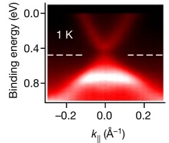
(b) Mn doped Bi₂Se₃

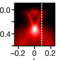
(c) Mn doped Bi₂Te₃

Figure 1: (a) Evolution of density of state as the doping changes. As we increase the doping the surface gap increases, and the fermi surface gets smaller. At some point, the surface band touches FS and the system become strongly interacting. The green colored region represent the the bulk bands and the lines are for surface bands. The figure is from Seo:2017yux . (b,c) The actual ARPES data for for Mn-doped Bi₂Se₃ and Bi₂Te₃. Notice that for the latter, it is hard to see the surface gap. The figure is from the ref.rienks2019large , https://rdcu.be/b3App

Then one may immediately ask whether we can still treat the system as a Dirac material, because strictly speaking, there is no more a Dirac cone. Therefore we have a pressing reason to re-examine the system with the hyper-scaling violating geometry. We will see that comparing our theoretical result to the data, the relevant QCP for this system should be identified as $(z,\theta)=(1.5,1)$ for Mn doped Bi₂Se₃ and $(z,\theta)=(1,0)$ for the Cr doped Bi₂Te₃.

Our analysis will also be useful for multilayer graphene system where the excitations are known to have dispersion relation $\omega=k^{n}$ PhysRevB.78.121401 .

We will see that the behavior of the transports can be qualitatively different, depending on the dynamical exponent of QCP. However, such difference can be recognized only by plotting the transports for various $(z,\theta)$, therefore we will put much efforts for explicitly plotting the result. We checked that our result in the limits of zero magnetic field and in the absence of the new coupling agrees with known result.

The rest of the paper consists of as follows. In section 2, we introduce the hyperscaling violation gravity model with a magnetic coupling and present its solution. In section 3, we calculate various transport coefficients. In section 4, we apply our result to the surface state of topological insulator with its charge carrier’s fermionic nature. In section 5, we conclude with summary. In appendices A and B, we give detailed study of the long and complicated formula by plotting the magneto transports and density dependence of the various QCP’s in order to explicitly show the presence of phase transitions across the four regions of critical exponents and the appearance of cross over from the weak localization to weak anti-localization. We also compared the magneto-transports without and with magnetic impurity. These are by themselves important since they are predictions that can be compared with future experimental data, but to avoid the too many figures in the main text, we put it at the appendices. At the end, we explain the null energy condition for our theory.

2 The model and its black hole solution

To get the solution with the dynamical exponent $z$ and the hyperscaling violating factor $\theta$, we consider a 4 dimensional action.

$$S_{tot} = \int_{\mathcal{M}}d^{4}x\left(\mathcal{L}_{0}+\mathcal{L}_{int}\right)$$

$$\mathcal{L}_{0} = \sqrt{-g}\left(R+\sum_{i=1}^{2}V_{i}e^{\gamma_{i}\phi}-\frac{1}{2}(\partial\phi)^{2}-\frac{1}{4}\sum_{i=1}^{2}Z_{i}(\phi)F_{(i)}^{2}-\frac{1}{2}Y(\phi)\sum\limits_{i,I}^{2}(\partial\chi_{I}^{i})^{2}\right)$$

$$\mathcal{L}_{int} = -\frac{q_{\chi}}{16}\sum_{I=1,2}(\partial\chi^{(2)}_{I})^{2}\epsilon^{\mu\nu\rho\sigma}F^{(2)}_{\mu\nu}F^{(2)}_{\rho\sigma},$$ (2)

where we will use the convention $2\kappa^{2}=16\pi G=1$. We use ansatz

$$Z_{i}=e^{\lambda_{i}\phi},\quad Y(\phi)=e^{-\lambda_{2}\phi},\quad\chi_{i}^{I}=\beta^{I}\delta_{Ii}x^{i},$$ (3)

where $\chi_{i}$’s are $d$-massless linear axions introduced to break the translational symmetry and $(\beta^{1},\beta^{2})=(\alpha,\lambda)$ denote the strength of momentum relaxation. The action consists of Einstein gravity, axion fields, and $U(1)$ gauge fields and a dilaton field. For simplicity, we only consider two $U(1)$ gauge $F^{(1)}_{rt}$ and $F^{(2)}_{rt}$ in which the first gauge field plays the role of an auxiliary field, making the geometry asymptotic Lifshitz, and the second gauge field is the exact Maxwell field making the black hole charged.

The equations of motion are given by

$$\partial_{\mu}(\sqrt{-g}g^{\mu\nu}Y(\phi)\sum_{a}\partial_{\nu}\chi^{(i)}_{I})+\frac{q_{\chi}}{8}\partial_{\mu}(\delta^{i2}\epsilon^{\rho\sigma\lambda\gamma}F^{(2)}_{\rho\sigma}F^{(2)}_{\lambda\gamma}g^{\mu\nu}\partial_{\nu}\chi^{(2)}_{I})=0,$$ (4)

$$\partial_{\mu}(\sqrt{-g}Z_{i}(\phi)F^{\mu\nu}_{(i)}+\frac{q_{\chi}}{4}\delta^{i2}g^{\rho\sigma}\sum_{I}\partial_{\rho}\chi^{(2)}_{I}\partial_{\sigma}\chi^{(2)}_{I}\epsilon^{\alpha\beta\mu\nu}F^{(2)}_{\alpha\beta})=0,$$ (5)

$$R_{\mu\nu}=\frac{1}{2\sqrt{-g}}g_{\mu\nu}\mathcal{L}_{0}+\frac{1}{2}\partial_{\mu}\phi\partial_{\nu}\phi+\frac{Y}{2}\sum_{i}\partial_{\mu}\chi^{(i)}_{I}\partial_{\nu}\chi^{(i)}_{I}+\frac{1}{2}\sum_{i}Z_{i}F_{(i)\mu}^{\rho}F_{\mu\rho}^{(i)}$$

$$+\frac{q_{\chi}}{16}\sum_{I}\frac{1}{\sqrt{-g}}(\partial_{\mu}\chi^{(2)}_{I})(\partial_{\nu}\chi^{(2)}_{I})\epsilon^{\rho\sigma\lambda\gamma}F^{(2)}_{\rho\sigma}F^{(2)}_{\lambda\gamma}.$$ (6)

$$\Box\phi+\sum_{i}V_{i}\gamma_{i}e^{\gamma_{i}\phi}-\frac{1}{4}\sum_{i}Z^{\prime}_{i}(\phi)F^{2}_{(i)}-\frac{1}{2}Y^{\prime}(\phi)\sum\limits_{i,I}^{2}(\partial\chi_{I}^{i})^{2}=0.$$ (7)

The solution for the dilaton field is given as

$$\phi(r)=\nu\ln r,\quad\hbox{with }\nu=\sqrt{(2-\theta)(2z-2-\theta)}.$$ (8)

The gauge couplings $Z_{1}$ and $Z_{2}$ can be solved to give

$$Z_{1}(\phi)=e^{\lambda_{1}\phi}=r^{\theta-4},\quad Z_{2}(\phi)=e^{\lambda_{2}\phi}=r^{2z-\theta-2},\quad Y(\phi)=1/Z_{2},$$ (9)

where $\lambda_{1}=(\theta-4)/\nu$ and $\lambda_{2}=\nu/(2-\theta)$. Other exponentials and potentials are

$$\gamma_{1}=\frac{\theta}{\nu},~{}~{}~{}\gamma_{2}=\frac{\theta+2z-6}{\nu},\quad V_{1}=\frac{z-\theta+1}{2(z-1)}(q_{1})^{2},~{}~{}~{}V_{2}=\frac{H^{2}(2z-\theta-2)}{4(z-2)},$$ (10)

where $H$ is a constant magnetic field. Finally, the solution is given by

$$A_{1}=a_{1}(r)dt,A_{2}=a_{2}(r)dt+\frac{1}{2}H(xdy-ydx),$$ (11)

$$\quad\chi^{(1)}_{I}=(\alpha x,\alpha y),\quad\chi^{(2)}_{I}=(\lambda x,\lambda y),$$ (12)

$$ds^{2}=r^{-\theta}\bigg{(}-r^{2z}f(r)dt^{2}+\frac{dr^{2}}{r^{2}f(r)}+r^{2}(dx^{2}+dy^{2})\bigg{)},$$ (13)

$$f(r)=1-mr^{\theta-z-2}-\frac{\beta^{2}}{(\theta-2)(z-2)}r^{\theta-2z}+\frac{q_{2}^{2}(\theta-z)r^{2\theta-2z-2}}{2(\theta-2)}$$

$$\qquad\qquad+\frac{H^{2}r^{2z-6}}{4(z-2)(3z-\theta-4)}+\frac{\lambda^{4}H^{2}q^{2}_{\chi}c_{3}}{r^{6+2z-4\theta}}-\frac{\lambda^{2}Hq_{2}q_{\chi}c_{2}}{r^{4+2z-3\theta}},$$ (14)

$$a_{1}(r)=\frac{-q_{1}}{2+z-\theta}(r_{\textrm{\tiny H}}^{2+z-\theta}-r^{2+z-\theta}),\;\;a_{2}(r)=\big{(}\mu-q_{2}r^{\theta-z}\big{)}-\frac{\lambda^{2}Hq_{\chi}c_{4}}{r^{z-2\theta+2}},$$ (15)

where $\beta^{2}=\alpha^{2}+\lambda^{2}$ and $c_{2}$, $c_{3}$, $c_{4}$ can be expressed in terms of $\theta$ and $z$

$$c_{2}=\frac{(z-\theta)}{(\theta-2)(2\theta-z-2)},\quad c_{3}=\frac{1}{2}\frac{1}{(2-\theta)(4+z-3\theta)},\quad c_{4}=\frac{1}{2\theta-z-2}.$$ (16)

The charge density is determined by the condition $a_{i}(r_{\textrm{\tiny H}})=0$ at the event horizon:

$$q_{1}=\sqrt{(2z-2)(2+z-\theta)},\quad q_{2}=\mu r_{\textrm{\tiny H}}^{z-\theta}-c_{4}\Theta H,$$ (17)

where $\Theta={\lambda^{2}q_{\chi}}/{r_{\textrm{\tiny H}}^{2-\theta}}.$ The entropy density and the Hawking temperature read

$$s= 4\pi r^{2-\theta}_{H},$$ (18)

$${4\pi}T= (z+2-\theta)r_{\textrm{\tiny H}}^{z}-\frac{\beta^{2}r_{\textrm{\tiny H}}^{\theta-z}}{2-\theta}-\frac{1}{2}\frac{r_{\textrm{\tiny H}}^{2\theta-2-z}}{(2-\theta)}\Big{(}\Theta H-(z-\theta)q_{2}\Big{)}^{2}-\frac{H^{2}r_{\textrm{\tiny H}}^{3z-6}}{4(2-z)}.$$ (19)

Notice that all three terms in eq. (19) contribute negatively and if both $z,\theta<2$ and at zero temperature, the solution near the horizon becomes $AdS_{2}\times R^{2}$:

$$ds^{2}=\frac{-d\tau^{2}+du^{2}}{l^{2}_{eff}u^{2}}+r_{\textrm{\tiny H}}^{2-\theta}(dx^{2}+dy^{2}).$$ (20)

We classify the plane of $(z,\theta)$ into several classes $O,I,II,III,IV$ depending on the behavior of the temperature as a function of $r_{H}$, the radius of the black hole which again is a complicated function of parameters of the theory. See Figure 2. I is the region which allows negative $T$. The region of $\theta>2$ has non-negative temperature, which can be further classified to three types II, III, IV. For III, temperature is monotonic function of $r_{H}$ and cover the entire positive temperature. For IV, there is a minimum temperature regardless of the chemical potential $\mu$. For II, depending on $\mu$, temperature has minimum like IV (real red curve in (b)) or monotonic like III (dotted red curve in (b)). we have two subclasses which are represented by solid (dashed) red curve for the case with the finite (vanishing) $\mu$. We do not have positive $T$ in region O.

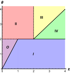
(a) Classification of $(z,\theta)$ space

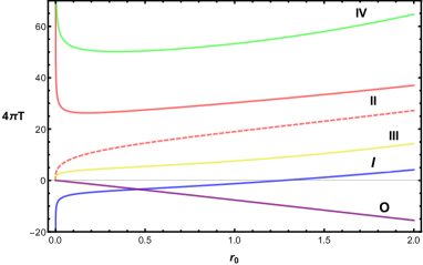
(b) $r_{0}$ $vs$ $T$

Figure 2: Classification of $(z,\theta)$ space by $T$-range: Each curves in (b) represent a typical curve of each region with the corresponding color of (a).

3 Calculation of magneto-transport coefficients

We calculate the transport following the idea of linear response theory. We consider the following perturbations

$$\delta g_{tx}=h_{tx}(r)+tf_{3x}(r),~{}~{}\delta g_{ty}=h_{ty}(r)+tf_{3y}(r),~{}~{}\delta g_{rx}=h_{rx}(r),~{}~{}\delta g_{ry}=h_{ry}(r),$$ (21)

$$\delta A_{ax}=b_{ax}-tf_{ax},~{}~{}\delta A_{ay}=b_{ay}-tf_{ay},\delta\chi_{1}=\varphi_{x}(r),\delta\chi_{2}=\varphi_{y}(r).$$ (22)

Requiring the linearised Einstein equations to be time-independent, we can get the explicit form of $f_{1i}$, $f_{2i}$, and $f_{3i}$ as

$$f_{1i}=-E_{1i}+\zeta_{i}a_{1}(r),$$

$$f_{2i}=-E_{2i}+\zeta_{i}a_{2}(r),$$

$$f_{3i}=-\zeta_{i}U(r)$$ (23)

The thermo-electric transport can be calculated at the event horizon. One can take the Eddington-Finkelstein coordinates $(v,r)$ such that the background metric is manifestly regular at the horizon,

$$ds^{2}=-Udv^{2}-2\sqrt{UV}dvdr+Wdx^{2}+Wdy^{2},$$ (24)

where $v=t+\int dr\sqrt{V/U}$. In this coordinate, the perturbed metric becomes

$$\delta g_{\mu\nu}dx^{\mu}dx^{\nu}=h_{tx}dvdx+h_{ty}dvdy+\bigg{(}h_{rx}-\sqrt{\frac{V}{U}}h_{tx}\bigg{)}drdx+\bigg{(}h_{ry}-\sqrt{\frac{V}{U}}h_{ty}\bigg{)}drdy.$$ (25)

In order to ensure the regularity of the perturbed metric at the horizon, we ask the vanishing of last two terms at the horizon so that

$$h_{ri}\sim\sqrt{\frac{V}{U}}h_{ti},\hbox{ with }i=x,y.$$ (26)

Similarly, we can expand the gauge fields in the Eddington-Finkelstein coordinates to get regularity condition at the horizon:

$$\delta A_{ai} \sim b_{ai}+E_{ai}v-E_{ai}\int dr\sqrt{\frac{V}{U}},$$ (27)

where $E_{ai}$ is constant probe electric fields with $a=1,2$ and $i=x,y$. The full gauge-field perturbation will have the regular expansion $\delta A_{ai}$ $\sim$ $E_{ai}v$ $+\cdots$ in the Eddington-Finkelstein coordinates, provided we demand

$$b^{\prime}_{ai}\sim\sqrt{\frac{V}{U}}E_{ai}.$$ (28)

To fix the perturbations, we need the linearized Einstein equations. The $(r,x)$ and $(r,y)$-components of the Einstein equation are given by

$$-\left(\frac{YV\beta^{2}}{W}+\frac{Z_{2}VH^{2}}{W^{2}}+\frac{q_{\chi}\lambda^{2}H\sqrt{UV}a_{2}^{\prime}}{UW^{2}}\right)h_{rx}+\frac{V}{U}\left(\sum_{i=1,2}\left(Z_{i}a_{i}^{\prime}f_{ix}\right)+f^{\prime}_{3x}\right)$$

$$\frac{Z_{2}VHa_{2}^{\prime}}{UW}h_{ty}-\frac{VW^{\prime}}{UW}f_{3x}+\frac{Z_{2}VH}{W}b_{2y}^{\prime}=0$$ (29)

$$-\left(\frac{YV\beta^{2}}{W}+\frac{Z_{2}VH^{2}}{W^{2}}+\frac{q_{\chi}\lambda^{2}H\sqrt{UV}a_{2}^{\prime}}{UW^{2}}\right)h_{ry}+\frac{V}{U}\left(\sum_{i=1,2}\left(Z_{i}a_{i}^{\prime}f_{iy}\right)+f^{\prime}_{3y}\right)$$

$$\frac{Z_{2}VHa_{2}^{\prime}}{UW}h_{tx}-\frac{VW^{\prime}}{UW}f_{3y}+\frac{Z_{2}VH}{W}b_{2x}^{\prime}=0$$ (30)

For simplification, it is fruitful to define following functions:

$$\mathcal{F} =WY\beta^{2}+Z_{2}H^{2}-q_{2}Y\Theta H+Y\Theta^{2}H^{2}$$

$$\mathcal{G} =q_{2}-\Theta H$$ (31)

where all the quantities are computed at $r=r_{H}$. For example, $W=W(r_{H})=r_{H}^{2-\theta}$. Regularity at the event horizon yields

$$h_{tx}|_{r_{H}}=-W\bigg{(}q_{1}(\mathcal{F}E_{1x}+\mathcal{G}E_{1y})+(\mathcal{F}-Z_{2}H^{2})\mathcal{G}E_{2x}+H(Z_{2}\mathcal{F}+\mathcal{G}^{2})E_{2y}$$

$$\qquad\quad+sT(\mathcal{F}\zeta_{x}+\mathcal{G}H\zeta_{y})\bigg{)}\bigg{/}(\mathcal{F}^{2}+H^{2}\mathcal{G}^{2})$$ (32)

$$h_{ty}|_{r_{H}}=-W\bigg{(}q_{1}(\mathcal{F}E_{1y}-\mathcal{G}E_{1x})+(\mathcal{F}-Z_{2}H^{2})\mathcal{G}E_{2y}-H(Z_{2}\mathcal{F}+\mathcal{G}^{2})E_{2x}$$

$$\qquad\quad+sT(\mathcal{F}\zeta_{y}-\mathcal{G}H\zeta_{x})\bigg{)}\bigg{/}(\mathcal{F}^{2}+H^{2}\mathcal{G}^{2})$$ (33)

The radially conserved electric current ${J}^{\mu}=(J^{t},J^{x},J^{y})$ can be defined by

$${J}_{a}^{\mu}=\sqrt{-g}Z_{(a)}F^{\mu r}_{(a)}+\frac{q_{\chi}}{4}\delta^{2a}g^{\rho\sigma}\sum_{I}\partial_{\rho}\chi^{(2)}_{I}\partial_{\sigma}\chi^{(2)}_{I}\varepsilon^{\alpha\beta\mu r}F^{(2)}_{\alpha\beta},$$ (34)

where the index $a=1,2$ denotes the two currents which are dual to the two gauge fields. One can define the ’conserved’ electric current ${\mathcal{J}}^{i}$ satisfying $\partial_{r}{\mathcal{J}}^{i}=0$ using the magnetization electric current ${\mathcal{M}}_{a}^{i}=\sqrt{-g}\partial_{j}(Z_{a}F_{(a)}^{ij}+\frac{q_{\chi}}{4}\delta^{2a}g^{\rho\sigma}\sum_{I}\partial_{\rho}\chi^{(2)}_{I}\partial_{\sigma}\chi^{(2)}_{I}\varepsilon^{\alpha\beta ij}F^{(2)}_{\alpha\beta})$ as follows,

$${\mathcal{J}}_{a}^{i}(r)=J_{a}^{i}(r)-\int_{r_{H}}^{r}dr{\mathcal{M}_{a}}^{i}(r).$$ (35)

Notice that ${\mathcal{J}}$ coincides with the local boundary current and it can be evaluated at the horizon. Then we get

$${\mathcal{J}}_{1i}=Z_{1}E_{1i}-\frac{q_{1}}{W}h_{ti}\bigg{|}_{r=r_{\textrm{\tiny H}}},$$ (36)

$${\mathcal{J}}_{2i}=Z_{2}E_{2i}-\frac{Z_{2}a^{\prime}_{2}}{UV}h_{ti}-\epsilon_{ij}\left(\frac{Z_{2}H}{W}h_{tj}-\frac{q_{\chi}\lambda^{2}E_{2j}}{\sqrt{UV}W^{2}}\right)\bigg{|}_{r=r_{\textrm{\tiny H}}},$$ (37)

For the transport coefficients, we will take only $J_{2i}$ and $E_{2i}$ as physical, because $A_{1i}$ is introduced just for constructing HSV geometry.

For the heat current, following Donos:2014cya , we introduce the total heat current $Q^{i}$ by

$$Q^{i}=2\sqrt{-g}G^{ri}$$ (38)

where the two form $G^{\mu\nu}$ is associated with the Killing vector $k=\partial_{t}$ by

$$G^{\mu\nu}=\nabla^{\mu}k^{\nu}+\frac{1}{2}\sum_{I=1,2}Z_{I}k^{[\mu}F_{I}^{\nu]\sigma}A_{I\sigma}+\frac{1}{4}\sum_{I=1,2}(Ex+2a_{I})Z_{I}F_{I}^{\mu\nu}.$$ (39)

It satisfies

$$\nabla_{\nu}G^{\mu\nu}=-Vk^{\mu}/2.$$ (40)

Then the heat current is given by Donos:2014cya ,

$${Q}^{i}=2\sqrt{-g}\nabla^{r}k^{i}-\sum_{I=1,2}a_{I}J_{I}^{i}=\frac{U^{2}}{\sqrt{UV}}(\frac{h_{ti}}{U})^{\prime}-\sum_{I=1,2}a_{I}J_{I}^{i}.$$ (41)

In the presence of the magnetic field, $\partial_{r}Q^{i}\neq 0$. In fact by taking $i$-th component of eq(40),

$$\partial_{r}Q^{i}=\partial_{j}G^{ij}:={\mathcal{M}}_{Q}^{i}.$$ (42)

Then the ’conserved’ heat current $\mathcal{Q}^{i}$ is defined by

$$\mathcal{Q}^{i}(r)=Q^{i}(r)-\int_{r_{H}}^{r}dr{\mathcal{M}}_{Q}^{i}(r),$$ (43)

It turns out that near the boundary, $\mathcal{Q}^{i}(r)\sim T^{ti}-\mu J^{i}$ which is the expected boundary heat current and ${\mathcal{M}}_{Q}^{i}$ gives the magnetization heat current for the charge and energy. Since $\mathcal{Q}^{i}$ is radially conserved, $\partial_{r}\mathcal{Q}^{i}=0$, it is enough to compute $\mathcal{Q}^{i}$ at the horizon.

$$\mathcal{Q}_{i}=-\frac{U^{\prime}h_{ti}}{\sqrt{UV}}({r_{H}}).$$ (44)

Finally we can read off the transport coefficients from the following matrix:

$$\left(\begin{array}[]{c}{\mathcal{J}}^{i}\\ {\mathcal{Q}}^{i}\end{array}\right)=\left(\begin{array}[]{cc}\sigma_{ij}&\alpha_{ij}T\\ \bar{\alpha}_{ij}T&\bar{\kappa}_{ij}T\end{array}\right)\left(\begin{array}[]{c}E_{j}\\ \zeta_{j}\end{array}\right),$$ (51)

where $\zeta_{j}=-(\nabla_{j}T)/T$ is the temperature gradient that drive thermal motion. The transport coefficients are given by

$$\sigma_{ii}=\frac{Z_{2}\left(\mathcal{F}+Y\mathcal{G}^{2}\right)\left(\mathcal{F}-Z_{2}H^{2}\right)}{\left(\mathcal{F}^{2}+H^{2}\mathcal{G}^{2}\right)},$$ (52)

$$\sigma_{ij}=\epsilon_{ij}\left(\Theta+\frac{Z_{2}H\mathcal{G}\left(2\mathcal{F}+Y\mathcal{G}^{2}-Z_{2}H^{2}\right)}{\left(\mathcal{F}^{2}+H^{2}\mathcal{G}^{2}\right)}\right),$$ (53)

$$\alpha_{ii}=\bar{\alpha}_{ii}=\frac{s\mathcal{G}\left(\mathcal{F}-Z_{2}H^{2}\right)}{\left(\mathcal{F}^{2}+H^{2}\mathcal{G}^{2}\right)},$$ (54)

$$\alpha_{ij}=\bar{\alpha}_{ij}=\epsilon_{ij}\frac{sH\left(Z_{2}\mathcal{F}+\mathcal{G}^{2}\right)}{\left(\mathcal{F}^{2}+H^{2}\mathcal{G}^{2}\right)},$$ (55)

$$\bar{\kappa}_{ii}=\frac{s^{2}T\mathcal{F}}{\left(\mathcal{F}^{2}+H^{2}\mathcal{G}^{2}\right)},$$ (56)

$$\bar{\kappa}_{ij}=\epsilon_{ij}\frac{s^{2}T\mathcal{G}}{\left(\mathcal{F}^{2}+H^{2}\mathcal{G}^{2}\right)},$$ (57)

The resitivity is defined as the inversion of the conductivity matrix:

$$\rho_{xx} = \frac{\sigma_{xx}}{\sigma_{xx}^{2}+\sigma_{xy}^{2}}=\mathcal{R}_{xx}/\mathcal{D},$$

$$\rho_{yx} = \frac{\sigma_{xy}}{\sigma_{xx}^{2}+\sigma_{xy}^{2}}=\mathcal{R}_{yx}/\mathcal{D},$$ (58)

where

$$\mathcal{R}_{xx} = Z_{2}(\mathcal{F}+Y\mathcal{G}^{2})(\mathcal{F}-Z_{2}H^{2}),$$

$$\mathcal{R}_{yx} = (\mathcal{F}^{2}+\mathcal{G}^{2}H^{2})\Theta+Z_{2}H\mathcal{G}(2\mathcal{F}+Y\mathcal{G}^{2}-Z_{2}H^{2}),$$

$$\mathcal{D} = (Z_{2}\mathcal{F}+\mathcal{G}^{2})^{2}+(\mathcal{F}^{2}+\mathcal{G}^{2}H^{2})\Theta^{2}+H(Z_{2}^{2}H-2\mathcal{G}\Theta)(Z_{2}^{2}H^{2}-2Z_{2}\mathcal{F}-\mathcal{G}^{2}).$$ (59)

The thermal conductivity when electric currents are turned off is given by

$$\kappa_{ij} = \bar{\kappa}_{ij}-T(\bar{\alpha}\cdot\sigma^{-1}\alpha)_{ij},$$ (60)

$$\kappa_{xx} = \mathcal{K}_{xx}/\mathcal{D},\qquad\kappa_{yx}=\mathcal{K}_{yx}/\mathcal{D},$$ (61)

where

$$\mathcal{K}_{xx} = s^{2}T(Z_{2}^{2}\mathcal{F}+Z_{2}\mathcal{G}^{2}-Z_{2}^{3}H+\mathcal{F}\Theta^{2}+2Z_{2}H\mathcal{G}\Theta),$$

$$\mathcal{K}_{yx} = s^{2}T(Z_{2}\mathcal{F}+\mathcal{G}^{2})(\mathcal{G}+H\Theta).$$ (62)

From these quantities, the Seebeck coefficient, $S$, and the Nernst signal, $N$, are given by

$$S =(\sigma^{-1}\cdot\alpha)_{xx}=\mathcal{S}/\mathcal{D},$$ (63)

$$N =(\sigma^{-1}\cdot\alpha)_{yx}=\mathcal{N}/\mathcal{D},$$ (64)

where

$$\mathcal{S} = s(Z_{2}\mathcal{F}+\mathcal{G}^{2})(\mathcal{G}+H\Theta),$$ (65)

$$\mathcal{N} = s(\mathcal{F}-Z_{2}H^{2})(\mathcal{G}\Theta-Z_{2}^{2}H).$$ (66)

The Hall angle is given by

$$\cot\theta_{H}=\frac{\sigma_{xx}}{\sigma_{xy}}=\frac{\mathcal{R}_{xx}}{\mathcal{R}_{yx}}=\frac{Z_{2}(\mathcal{F}+Y\mathcal{G}^{2})(\mathcal{F}-Z_{2}H^{2})}{(\mathcal{F}^{2}+\mathcal{G}^{2}H^{2})\Theta+Z_{2}H\mathcal{G}(2\mathcal{F}+Y\mathcal{G}^{2}-Z_{2}H^{2})}.$$ (67)

Our result resembles the result of Dirac material because we could find $\mathcal{F}$ and $\mathcal{G}$ given by eq(3). However, transport behavior is expected to depend on the class of exponent. In fact, for $z=1$, the system becomes strongly interacting due to the small fermi surface, while higher exponents cases are strongly interacting because the band is flat. Since the mechanisms for the strong correlation are different, we do have reason to expect the difference between the Dirac and non-Dirac materials in transport coefficients as well as the band structure.

Before exploring such aspect of transports, it will be convenient to divide regions of $(\theta,z)$ as Figure 3. One can see from eq 11 that there’s singularities at $z=2$ and $\theta=2$ . Therefore, there must be a rapid change in the transport behavior along this boundaries. We also have some restrictions on the $(z,\theta)$ which is determined by the following conditions:

• The reality condition of $q_{1}$ (17): $(2z-2)(2+z-\theta)\geq 0$

• Null energy condition (NEC): ${(2-\theta)(2z-2-\theta)}\geq 0.$ See appendix (104).

• The condition that the background solution has hyperscaling violating geometry at the asymptotic boundary.

The regime which satisfies above three conditions is described in Figure 3 (b).

(a) Phases of transports

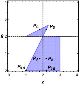
(b) Validity regime

Figure 3: (a) 4-phases A,B,C,D due to the sign changes at $z=2$ and $\theta=2$. (b) Valid region satisfying all three conditions: (i) $q_{1}$ charge reality condition, (ii) Null energy condition, (iii) Asymptotic HSV condition. Black dots indicate specific $(z,\theta)$ where we will discuss the typical behavior of transports from next section

In the appendices, we will examine the behaviors of transports in detail by plotting and analytic analysis and we will see that there are phase transitions at the phase boundaries of A,B,C,D due to the singularities sitting there. Also there are crossovers from weak localization to anti-localizations whose boundaries are rather complicated. Although we list these plotting at the appendix to avoid too many figures in the main text, they are important by themselves because the plots are predictions that can be easily compared with experiments. We will provide one such comparison in the next section.

4 Application: magnetically doped surface state of topological insulator

We now apply the result to the surface state of topological insulator with gap opened by the magnetic dopingzhang2012interplay , which was one of our main motivation. After extensive search, it turns out that the best fit comes from $(z,\theta)=(3/2,1)$, which we call QCP $Q_{2}$. As we move away from $(3/2,1)$, the fitting becomes bad very rapidly as one can see in the figure 4(b,c,d). Therefore there is no ambiguity in associating the surface state of Mn doped Bi₃Se₃ with a QCP with $(z,\theta)=(3/2,1)$.

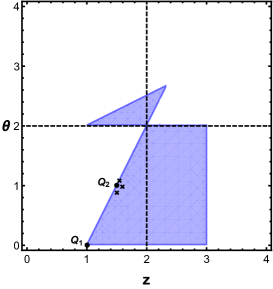
(a) $Q_{2}$ and its 3 nearby QCP’s

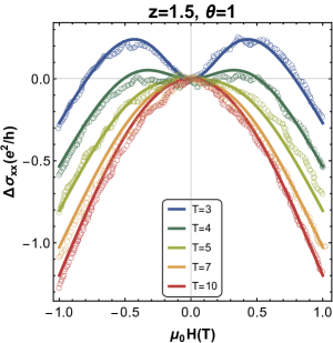
(b) At $Q_{2}$

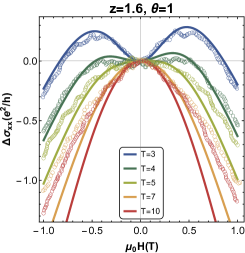
(c) right of $Q_{2}$

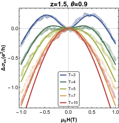
(d) below $Q_{2}$

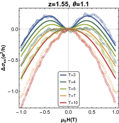
(e) above $Q_{2}$

Figure 4: (a) Two quantum critical point $Q_{1},Q_{2}$: $Q_{1}$ is for Cr doped Bi₂Te₃ discussed in Seo:2017oyh and $Q_{2}$ is for Mn doped for Bi₂Se₃ which is the topic here. (b,c,d,e) The uniqueness of $Q_{2}$, the QCP with $(z,\theta)=(3/2,1)$. The data is for Mn_0.04(Bi₂Se₃)_0.96 taken from ref. zhang2012interplay . Solid line and circles are for theory curve and experimental data respectively. The fitting is good at $Q_{2}$ as one can see in (b). But as we deviate from it, the fitting becomes bad rapidly for high temperature data. See (c,d,e).

In each figure of 4(b,c,d,e) we first fix the parameters such that the theory best fit the $T=3$K data (blue line), then we use them for data at other temperatures. The parameters used in figure 4 are listed in table 1.

Table 1: Used parameters in figure 4

	$(z,\theta)$	$\beta^{2}(\mu m)^{2}$	$v/(10^{4}m/s)$	$q_{\chi}\gamma$
(a)	(1.5,1)	2704	5	3.1
(b)	(1.6,1)	2591	4.3	2.6
(c)	(1.5,0.9)	3136	5	2.15
(d)	(1.5,1.1)	3136	5	3.3

Here should comments on the material dependence of the QCP. Previously we could fit the data of Cr doped Bi₂Te₃ with $z=1,\theta=0$ Seo:2017oyh . There, we also claimed that the data of Mn doped Bi₂Se₃ can also be fit with $(z,\theta)=(1,0)$. However, it turns out that when we fix the parameters of the theory such that we can fit the data at low temperature (T=3K), higher temperature data of Bi₂Te₃ could be fit only if we allow the temperature dependence of the coupling $q_{\chi}$, while the theory can fit the data without such tweaking if we use $(z,\theta)=(3/2,1)$.

What is the origin of the difference between the two surface state? First the surface gap of doped Bi₂Se₃ is much bigger than that of doped Bi₂Te₃. The former has stronger Coulomb interaction between the electrons rienks2019large so that the system behaves as a strongly interacting system even at low doping. On the other hand, doped Bi₂Te₃ is a weakly interacting system at low doping. The surface Dirac point of Bi₂Te₃ is hidden in the valley of bulk band. It is hard to see the presence of the surface gap out of ARPES data while the surface gap is manifest for the doped Bi₂Te₃. See the figure 1(b and c). Therefore the two surface states are very different as QCP’s although they apparently look similar as surface states of TI.

Finally we remark that quantum critical point appears only at special dopings depending on the base material. We demonstrate this by showing that among three doping inverse ratio Bi/Mn=23.6, 12.5, 10.6 only the first data could be fit by our theory. See figure 5. In all three cases, we fix the theory parameter to fit the lowest temperature T=3K. We tabulated the parameters we used in table 2. If there were a scaling behavior, the same parameter set should able to fit the all data. Only Bi/Mn=23.6 data has such scaling property. That is only this case is at or near a QCP.

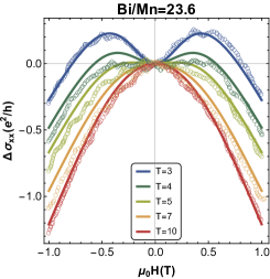
(a) At or near QCP

(b) Far from the QCP

(c) Farther from the QCP

Figure 5: QCP appears only at special dopings depending on the base material, where the data can be described by our theory.

Table 2: Used parameters in figure 5

	Bi/Mn	$\beta^{2}(\mu m)^{2}$	$v/(10^{4}m/s)$	$q_{\chi}\gamma$
(a)	23.6	2704	5	3.1
(b)	12.5	4096	6.67	2.7
(c)	10.3	4502	6.67	0.7

5 Conclusion and discussions

In this paper we reported a new black hole solution with hyperscaling violation which is relevant to an impurity doped quantum materials. We calculated all transport coefficients including electrical, thermo-electric and heat conductivities. We investigated their properties in detail by plotting the analytic results as a function of physical parameters. We also investigated the phase transitions from weak localization to weak anti-localization as the critical exponent changes.

In the introduction we mentioned the physics of the surface state of topological insulator with magnetic doping. It turns out that there are many subtle issues in discussing the physics of QCP related to the data of topological surfaces: for example, the Dirac cone at the surface of the TI is due to the zero-mode soliton, which should be distinguished from a local fermions. It is the consequence of collective motion of many electrons and it is not clear whether we can consider them as fermions satisfying the Pauli principle. We hope we can treat this issue in future work.

One interesting question is whether we can find a strange metal properties where resistivity $\sim T$ and Hall angle $\Theta\sim 1/T^{2}$ for some exponent. It turns out that the relevant point is $(z,\theta)=(1,1)$. However it is out of the stability condition requested by the null energy condition, explained in appendix C. It is too early to abandon such regime, since we did not in-cooperate the presence of the neutralizing ionic charges into gravitational context.

Finally the most interesting project would be the matching the gravity solutions with real systems, which would request collecting all available data. We wish to come back to this issue soon.

Appendix A Magneto-transports vs Quantum critical points

In this section, we discuss the typical behaviors of magneto-transport by taking a point from each sector A,B,C,D of the Figure 3(a). We take two more points along the $\theta=0$ line. Notice that the transverse quantities $\sigma_{xy}$, $\kappa_{xy}$, and $S$ vanish when $q_{\chi}=\mu=0$. We used $\alpha=0$ and $\beta=\lambda=1.3$.

A.1 Classifying the magneto-conductivity in $(z,\theta)$ plane

Figure 6 shows the temperature evolution of magneto-conductivity.

(a) $P_{0A}$ at $q_{\chi}=0$

(b) $P_{0A}$ at $q_{\chi}=0.7$

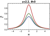
(c) $P_{0B}$ at $q_{\chi}=0$

(d) $P_{0B}$

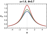
(e) $P_{A}$ at $q_{\chi}=0$

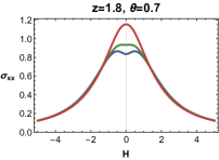
(f) $P_{A}$

(g) $P_{B}$ at $q_{\chi}=0$

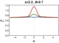
(h) $P_{B}$

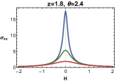
(i) $P_{C}$ at $q_{\chi}=0$

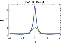
(j) $P_{C}$

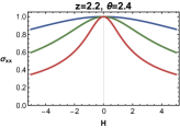
(k) $P_{D}$ at $q_{\chi}=0$

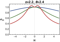
(l) $P_{D}$

Figure 6: Temperature evolution for $\sigma_{xx}(H)$ for different $(z,\theta)$. Each curves corresponds to $T=0.04,0.1,0.24$ for blue, green, and red respectively. We used $q_{\chi}=0.7$ for all non-zero $q_{\chi}$ case.

There are several interesting features for longitudinal electric conductivity, which we will understand by analytic calculations later :

• For the regions A and B, $\sigma^{0}_{xx}$, the longitudinal conductivity at $H=0$, increases as a function of temperature while it decreases in phase C and D. Such opposite behaviors are characters for other transport coefficients also. See figure 6.

• For the regions B, C, the longitudinal electric conductivity has finite values at $H\rightarrow\infty$. It happens only when magnetic impurity $q_{\chi}\neq 0)$.

• At the NEC boundary in the region $A$, weak localizations appear at low temperature, while it appears at high temperature at the NEC boundary in $D$.

Although the longitudinal electric conductivity is very complicated, we can understand a few important aspects in the limit of small and large $H$. For $H=q_{2}=0$,

$$\sigma_{xx}|_{H=0}\equiv\sigma_{xx}^{0}=r_{0}^{2z-\theta-2}.$$ (68)

where $r_{0}$ is $r_{H}$ at $H=q=0$. The temperature behavior of $\sigma_{xx}^{0}$ is different for each region in $z$-$\theta$ plane. At $H=0$,

$$4\pi T|_{H=0}=r_{0}^{z}(2+z-\theta)+\frac{r_{0}^{\theta-z}\beta^{2}}{\theta-2}.$$ (69)

The first term in (69) is dominant for high temperature if $\theta<2z$, while the second term is dominant if $\theta>2z$. In the region $A$ and $B$ satisfying NEC $(\theta<2z-2)$, $\theta$ is always smaller than $2z$ so that $T\sim r_{H}^{z}$, then

$$\sigma_{xx}^{0}\sim T^{\frac{2z-\theta-2}{z}},$$ (70)

which is an increasing function of temperature. This explains the temperature dependence of $\sigma_{xx}^{0}$ in Figure 6 (c) - (h).

The eq. (69) suggests that the regions $C$ and $D$ might be divided into two parts. When $\theta<2z$, the first term in (69) is dominant and hence $\sigma_{xx}^{0}$ follows the form of (70) but the exponent is negative by NEC. For $\theta>2z$, we have

$$\sigma_{xx}^{0}\sim T^{\frac{2z-2-\theta}{\theta-z}},$$ (71)

whose exponent is again negative when $\theta>2z$. Therefore, in the region $C$, $D$, $\sigma_{xx}^{0}$ decreases with temperature regardless of sign of $\theta-2z$. This explains the temperature dependence of $\sigma_{xx}^{0}$ in Figure 6 (i) and (j). There is the special case when $(z,~{}\theta)$ lies on the boundary of NEC, $2z-2-\theta=0$, where $\sigma^{0}_{xx}=1$ is independent of $T$ by (68), explaining Figure 6 (a), (b), (k) and (l).

So far, we discussed the behavior of the longitudinal conductivity in the absence of the external magnetic field. When the magnetic field is finite, the relation between temperature and $r_{H}$ is rather complicated as one can see in (19) and the analytic expression of $r_{H}$ in terms of other parameters is not available. But in the small $H$ limit, $H$ dependence of $r_{H}$ for fixed parameters $(T,\beta,~{}\lambda,~{}\theta,~{}z)$ can be obtained using

$$\frac{\delta r_{H}}{\delta H} =-\frac{(\theta-2)\left[r_{0}^{4z}(2+z-2\theta)^{2}+2q_{\chi}^{2}\lambda^{4}r_{0}^{4\theta}(z-2)(\theta-2)\right]H}{2r_{0}^{5}(z-2)(2+z-2\theta)^{2}\left[r_{0}^{2}z(2z-\theta)(\theta-2)+\beta^{2}r_{0}^{\theta}(\theta-z)\right]}+{\cal O}(H^{3})$$ (72)

$$\equiv{\cal A}_{1}H+{\cal O}(H^{3}),$$ (73)

where $r_{0}$ is $r_{H}(H=q=0)$.

Now, we have small $H$ expansion of $\sigma_{xx}$ as

$$\sigma_{xx}=\sigma_{xx}^{0}-\frac{r_{0}^{2z-2\theta-8}}{2}\left[\frac{2r_{0}^{4z}}{\beta^{2}}-{\cal A}_{1}(2z-\theta-2)r_{0}^{\theta+5}-\frac{2q_{\chi}^{2}\lambda^{4}r_{0}^{4\theta}(1+z-2\theta)^{2}}{\beta^{2}(2+z-2\theta)^{2}}\right]H^{2}+\cdots.$$ (74)

Depending on the sign of the coefficient of $H^{2}$, the system has weak anti-localization (WAL) for $-$ sign or weak localization (WL) for + sigin. When $(z,~{}\theta)$ parameters are off the NEC boundary, the coefficient of $H^{2}$ in (74) is complicated function of $z$, $\theta$ and other parameters, but there still exists competition between the two terms which lead to the transition from WL to WAL. Figure 7 is the phase diagram where yellow region denotes WL (positive sign) and gray region corresponds to WAL (negative sign). Dotted line is the boundary of the validity regime in Figure 3 (b). In the absence of $q_{\chi}$ most part of validity regime starts with WAL pahse. Small region near $z=2$ in $A$ and $D$ has WAL. As $q_{\chi}$ increases, the region of WL expands in the regions A, B and D while region C still remains in WAL. As temperature increases, yellow regions in $A$, $B$ shrink and finally disappear, which means that the longitudinal conductivity shows weak anti-localization(WAL) behavior at high temperature. On the other hand, the yellow regions in $C$, $D$ expand and fill the whole region of $C$, $D$ at high temperature.

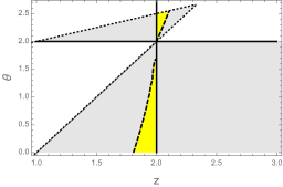
(a) $q_{\chi}=0$

(b) $q_{\chi}=0.7$

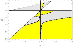
(c) $q_{\chi}=1.4$

Figure 7: WL (yellow) vs WAL(gray) in the validity regime. Other parameters are same as in Figure 6 and $T=0.04$.

For special case where $(z,~{}\theta)$ at the boundary of NEC ($\theta=2z-2$), the (74) has simpler form:

$$\sigma_{xx} =\sigma_{xx}^{0}-\frac{r_{0}^{2z-4}}{\beta^{2}}\left[1-\frac{q_{\chi}^{2}\lambda^{4}(3z-5)^{2}}{(3z-6)^{2}}r_{0}^{4z-8}\right]H^{2}+\cdots.$$ (75)

In the absence of $q_{\chi}$ (75) shows weak anti-localization behavior, while it changes to weak localization behavior when $q_{\chi}\lambda^{2}$ is large. For the given value of $q_{\chi}\lambda^{2}$, temperature behavior depends on $z$ and $\theta$. At the NEC boundary, the first term in (69) is dominant and hence $r_{H}\sim T^{1/z}$. Then coefficient of $H^{2}$ in (75) behaves

$$\Delta\sigma_{xx} \sim-(1-c_{*}T^{4-\frac{8}{z}}),$$ (76)

with a positive constant $c_{*}$, which means that weak anti-localization appears at low temperature at the NEC boundary in A region $z<2$ but appears at high temperature at the NEC boundary in D $(z>2)$. See Figure 6 (b) and (l).

Another interesting phenomena in the region B and C is that $\sigma_{xx}$ goes to constant for large magnetic field $H$ as one can see in Figure 6 (d), (h) and (j). To understand this, we first notice that large $H$ behavior of the conductivity is entirely determined by that of $r_{H}$, because eq. (52) says that both numerator and denominator have explicit $H^{4}$ behavior so that in this limit the conductivity is determined only by the $H$ dependence of $r_{H}$. From the expression of eq.(19),

$$r_{H}=r_{\infty}+\frac{C}{H^{2}}+\cdots,\hbox{ for }H\to\infty$$ (77)

in the relevant regions. Namely, if $r_{\infty}$ is well defined, the noted behavior is explained. Starting with the $H$ expansion of eq.(19),

$$4\pi T=-\left(\frac{r_{H}^{2\theta-2-z}\Theta^{2}}{2(2-\theta)}+\frac{r_{H}^{3z-6}}{4(z-2)}\right)H^{2}+\cdots,$$ (78)

In order for the left hand side to be finite, the coefficients of $H^{2}$ should vanish. Therefore

$$r_{H}^{4z-2\theta-4}=2\left(\frac{z-2}{2-\theta}\right)\Theta^{2}>0$$ (79)

requesting

$$(z-2)(\theta-2)<0,$$ (80)

which is precisely the equation defining the region $B$ and $C$.

Now we consider transverse magneto-conductivity. Figure 8 shows external magnetic field dependence of $\sigma_{xy}(H)$. Because we are considering only zero chemical potential case, the transverse conductivity vanishes in the absence of $q_{\chi}$, which means that the transverse conductivity is generated by the $q_{\chi}$ interaction term. This can be understood by the fact that $q_{\chi}$ term generates finite magnetization as well as the effective charge carrier by (17) and therefore transverse movement of charge carriers is also generated.

We can also expand $\sigma_{xy}$ in small magnetic field limit as previous discussion,

$$\sigma_{xy}=\sigma_{xy}^{0}-\frac{q_{\chi}\lambda^{2}}{2r_{0}^{8}}\left[\frac{4r_{0}^{4z}(1+z-2\theta)}{\beta^{2}(2+z-2\theta)}-(\theta-2){\cal A}_{1}r_{0}^{\theta+5}\right]H^{2}+\cdots,$$ (81)

where ${\cal A}_{1}$ is defined in (72).

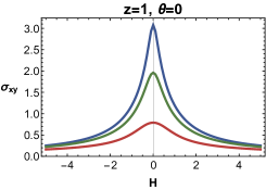
(a) $P_{0A}$

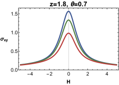
(b) $P_{A}$

(c) $P_{C}$

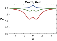
(d) $P_{0B}$

(e) $P_{B}$

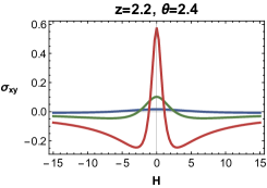
(f) $P_{D}$

Figure 8: Temperature evolution for $\sigma_{xy}(H)$ for different $(z,\theta)$. Curves correspond to $T=0.04,0.1,0.24$ for blue, green, and red respectively. We used $q_{\chi}=0.7$.

$\sigma_{xy}^{0}$ is called ‘anomalous Hall conductivity’ which is the transverse conductivity in the absence of the external magnetic field. It is given by

$$\sigma_{xy}^{0}=q_{\chi}\lambda^{2}r_{0}^{\theta-2}.$$ (82)

Using the similar analysis as before, we found that that $\sigma_{xy}^{0}$ is a decreasing function of temperature in the region $A$, $B$ but increasing function in the region $C$ and $D$.

The second term in (81) determines curvature of the transverse conductivity near $H=0$ which is not easy to analyze. We checked numerically that the sign of the second term is always negative in all region. The result is given by the Figure 9. We find that the region of WAL and WL is insensitive of the value of $q_{\chi}$.

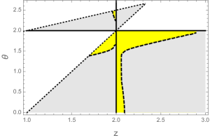
Figure 9: Sign of the coefficient of $H^{2}$ of the transverse conductivity near $H=0$. Yellow region denotes positive sign and gray region is for negative sign. Dotted line indicates validity regime. Here we use the parameters of Figure 8 and $T=0.1$.

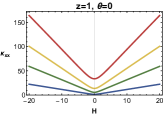
(a) $P_{0A}$ at $q_{\chi}=0$

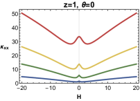
(b) $P_{0A}$

(c) $P_{0B}$ at $q_{\chi}=0$

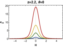
(d) $P_{0B}$

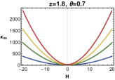
(e) $P_{A}$ at $q_{\chi}=0$

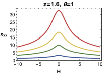
(f) $P_{A}$

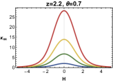
(g) $P_{B}$ at $q_{\chi}=0$

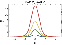
(h) $P_{B}$

(i) $P_{C}$ at $q_{\chi}=0$

(j) $P_{C}$

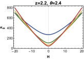
(k) $P_{D}$ at $q_{\chi}=0$

(l) $P_{D}$

Figure 10: Temperature evolution for $\kappa_{xx}(H)$ for different $(z,\theta)$. Each curve corresponds to $T=0.04,0.1,0.16,0.24$ for blue, green, yellow and red respectively. We used $q_{\chi}=0.7$ for all non-zero $q_{\chi}$ case.

A.2 Classifying the magneto-thermal conductivity in $(z,\theta)$ plane

In this section, we will discuss magneto-thermal conductivities. Figure 10 shows the external magnetic field dependence of the thermal conductivity given in (60). In the small $H$ limit, the longitudinal thermal conductivity can be expanded as

$$\kappa_{xx}=\kappa_{xx}^{0}-\frac{16\pi^{2}r_{0}^{2z-2\theta-6}T}{\beta^{4}}\left[r_{0}^{5}\beta^{2}(\theta-z){\cal A}_{1}+{\cal B}_{1}\right]H^{2}\cdots,$$ (83)

where ${\cal A}_{1}$ is defined in (72) and

$$\kappa_{xx}^{0} =\frac{16\pi^{2}r_{0}^{2(z-\theta)}}{\beta^{2}}T$$ (84)

$${\cal B}_{1} =\frac{q_{\chi}^{2}\lambda^{4}r_{0}^{3\theta}}{(2+z-2\theta)^{2}}\left[(1+z-2\theta)(2+z-2\theta)+\frac{1}{1+q_{\chi}^{2}\lambda^{4}r_{0}^{-4z+4\theta}}\right].$$ (85)

The temperature dependence of $\kappa_{xx}^{0}$ can be understood using the same analysis we used for the electric conductivity. In the region $A$ and $B$, horizon radius $\sim T^{1/z}$ and $z>\theta$. Therefore, $\kappa_{xx}^{0}$ increases at high temperature. One can easily check that the exponent becomes negative in the region $C$ and $D$ and hence $\kappa_{xx}^{0}$ is suppressed at high temperature.

The coefficient of $H^{2}$ in (83) determines a shape of the thermal conductivity near $H=0$. However, the coefficient is too complicated function for analytic approaches. The numerical result for the sign of the coefficient of $H^{2}$ is drawn in Figure 11, where yellow region denotes the positive sign corresponding to the weak localization. Gray region corresponds to the negative sign and weak anti-localization. In region $B$ and $C$, the coefficient is always negative but in region $A$ and $D$, there are domains of positive sign. In the absence of $q_{\chi}$. the region $A$ and $D$ are filled with WL as shown in the Figure 10. As we increase $q_{\chi}$, the region of WAL start to appear and increases. But the shape is complicated. The sign of the coefficient is positive near $z=2$ and turns to negative at other region. See Figure 11. Figure 12 demonstrates the phase transition from WL to WAL due to the sign flip of $H^{2}$ coefficient.

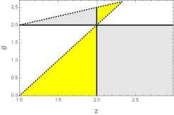
(a) $q_{\chi}=0$

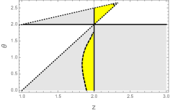
(b) $q_{\chi}=0.7$

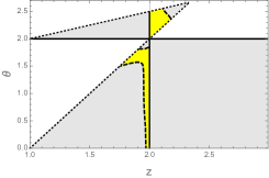
(c) $q_{\chi}=1.4$

Figure 11: Sign of the coefficient of $H^{2}$ of the thermal conductivity near $H=0$. Yellow region denotes positive sign(WL) and gray region is for negative sign(WAL). Dotted line is for NEC. Here we use the same parameter of Figure 10 and $T=0.16$.

(a) WL

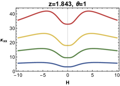
(b) Near phase boundary

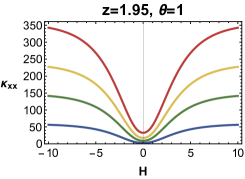
(c) WAL

Figure 12: Phase transition from WL to WAL behavior of $\kappa_{xx}(H)$ as $z$ increases along $\theta=1$ line. The transition occur near $z=1.843$. Curves corresponds to $T=0.04,0.1,0.16,0.24$ for blue, green, yellow, and red respectively. We used $q_{\chi}=0.7$.

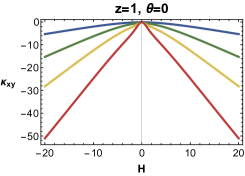
(a) $P_{0A}$

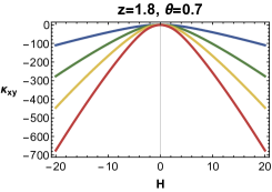
(b) $P_{A}$

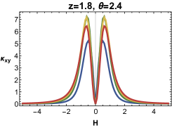
(c) $P_{C}$

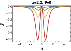
(d) $P_{0B}$

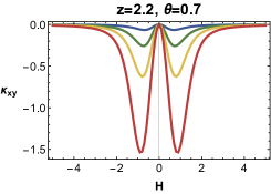
(e) $P_{B}$

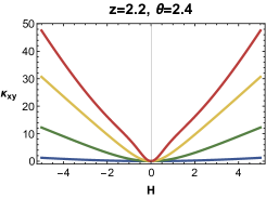
(f) $P_{D}$

Figure 13: Temperature evolution for $\kappa_{xy}(H)$ for different $(z,\theta)$. Each curves corresponds to $T=0.04,0.1,0.16,0.24$ for blue, green, yellow, and red respectively. We used $q_{\chi}=0.7$.

The transverse thermal conductivity can be expanded for small $H$ as

$$\kappa_{xy}=-\frac{16\pi^{2}q_{\chi}\lambda^{2}r_{0}^{4z-\theta-6}}{\beta^{4}}\,\left[\frac{(2+z-2\theta)r_{0}^{4z}+q_{\chi}^{2}\lambda^{4}(1+z-2\theta)r_{0}^{4\theta}}{(2+z-2\theta)^{2}(r_{0}^{4z}+q_{\chi}^{2}\lambda^{4}r_{0}^{4\theta})}\right]H^{2}+\cdots.$$ (86)

When $q_{\chi}=0$, the sign of coefficient is only depends on the sign of $-(2+z-2\theta)$ because all other terms are positive definite. This sign is negative in region $A$, $B$ and positive in $C$, $D$. The full magnetic field dependence of the transverse thermal conductivity is drawn in Figure 13. When we turn on $q_{\chi}$, the second term can change the value of $(z,~{}\theta)$ where the sign of the coefficient flipped. Numerical calculation indicates that the sign of $H^{2}$ changes near $(z,~{}\theta)=(2,2)$ in the region $A$, $B$. This region increase as $q_{\chi}$ increases, see Figure 14 (a).

(a) $\kappa_{xy}(q_{\chi}=0.7)$

(b) $\kappa_{xy}(q_{\chi}=1.4)$

(c) $N(q_{\chi}=0.7)$

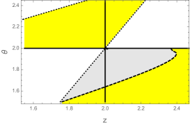
(d) $N(q_{\chi}=1.4)$

Figure 14: (a,b) WL vs WAL in thermal conductivity. (c,d) WL vs WAL in Nernst signal. They are determined by sign of the coefficient of $H^{2}$ in case of $\kappa_{xy}$ or $H$ in case of N. Yellow region denotes positive sign(WL) and gray region is for negative sign(WAL). Dotted line is for NEC. Here we use the same parameter of figures and $T=0.24$.

Figure 15 and Figure 16 show the external magnetic field dependence of the Seebeck coefficient and Nernst signal which are related to the thermoelectric conductivity $\alpha_{ij}$. These quantities have different behavior from the other transport coefficients. They are odd function of the magnetic field. The small field expansion of the Seebeck coefficient and Nernst signal become

$$N \sim\frac{4\pi r_{0}^{2z-\theta-2}}{\beta^{2}}\left[\frac{(2+z-2\theta)r_{0}^{4z}+q_{\chi}^{2}\lambda^{4}(1+z-2\theta)r_{0}^{4\theta}}{(2+z-2\theta)(r_{0}^{4z}+q_{\chi}^{2}\lambda^{4}r_{0}^{4\theta})}\right]H+\cdots,$$ (87)

$$S \sim\frac{4\pi}{\beta^{2}}\,\frac{q_{\chi}\lambda^{2}r_{0}^{4z+\theta-2}}{(2+z-2\theta)(r_{0}^{4z}+q_{\chi}^{2}\lambda^{4}r_{0}^{4\theta})}H+\cdots,$$ (88)

which are enough to explain the linearity of $N$ and $S$ near $H=0$ in the figures 15 and 16. In the absence of $q_{\chi}$, the slop of Nernst signal is alway positive, but it can be negative depending on the value of $q_{\chi}$. The coefficient of $H$ is same as the coefficient of $H^{2}$ of the transverse thermal conductivity (86) with opposite sign. Therefore, the region where the sign changes should be the same as $\kappa_{xy}$. See Figure 14 (b).

The sign of the slope of Seebeck coefficient only depends on $(2+z-2\theta)$ in the denominator. Together with NEC, the sign is positive in the region $A$, $B$ and negative in $C$, $D$.

(a) $P_{0A}$ at $q_{\chi}=0$

(b) $P_{0A}$

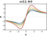
(c) $P_{0B}$ at $q_{\chi}=0$

(d) $P_{0B}$

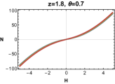
(e) $P_{A}$ at $q_{\chi}=0$

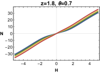
(f) $P_{A}$

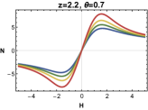
(g) $P_{B}$ at $q_{\chi}=0$

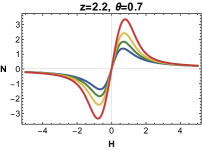
(h) $P_{B}$

(i) $P_{C}$ at $q_{\chi}=0$

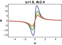
(j) $P_{C}$

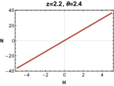
(k) $P_{D}$ at $q_{\chi}=0$

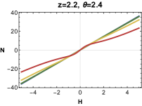
(l) $P_{D}$

Figure 15: Temperature evolution for $N(H)$ for for each region of $(z,\theta)$. Curves corresponds to $T=0.04,0.1,0.16,0.24$ for blue, green, yellow, and red respectively. We used $q_{\chi}=0.7$ for all non-zero $q_{\chi}$ case.

In the figure 15, we draw the temperature evolution for $N(H)$ for different $(z,\theta)$ which are denoted as big dots in the figure 3(b). In the figure 16, we draw the temperature evolution for $S(H)$ for different $(z,\theta)$ which are denoted as big dots in the figure 3(b).

(a) $P_{0A}$

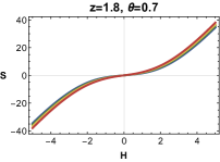
(b) $P_{A}$

(c) $P_{C}$

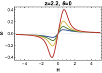
(d) $P_{0B}$

(e) $P_{B}$

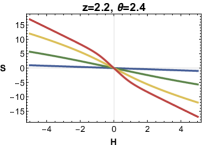
(f) $P_{D}$

Figure 16: Temperature evolution for $S(H)$ for each region of $(z,\theta)$. Each curves corresponds to $T=0.04,0.1,0.16,0.24$ for blue, green, yellow, and red respectively. In all figure we used $q_{\chi}=0.7$.

Appendix B Density dependence of Transports

In this section, we discuss the $q_{2}$, density, dependence of transport coefficients. For the ease of the analysis we consider only only zero external magnetic field cases. Notice that $\rho_{yx}$, $\kappa_{xy}$, and $N$ vanish when $q_{\chi}=0$ and $H=0$.

In the regions A and B, the longitudinal electric conductivity has a scaling behavior for large density, namely, $\gamma=\partial(\log\sigma_{xx})/\partial(\log q_{2})$ is a constant at $q_{2}\rightarrow\infty$. To see this, we consider the temperature at $H=0$:

$$4\pi T=r_{H}^{z}(2+z-\theta)+\frac{q_{2}^{2}r_{H}^{-z-2+2\theta}(z-\theta)^{2}}{2(\theta-2)}+\frac{r_{H}^{\theta-z}\beta^{2}}{\theta-2}.$$ (89)

In regions A and B satisfying NEC, $\theta<2z$ so that we can neglect the third term for large $q_{2}$. For the regions A and B where $\theta<2$, we have $r_{H}\sim q_{2}^{\frac{1}{z-\theta+1}}$. Rewriting the longitudinal conductivity from eq (52) with this horizon behavior for large density,

$$\sigma_{xx}=r_{H}^{2z-4}\left(r_{H}^{2-\theta}+\frac{q_{2}^{2}}{\beta^{2}}\right)\sim q_{2}^{\gamma}\qquad\text{with}\qquad\gamma=\frac{2(2z-\theta-1)}{z-\theta+1}.$$ (90)

Notice that the first term in (90) is subleading so the behavior is governed by the explicit $q^{2}$ dependent term. Fig. 17 demonstrate the scaling behavior of $\sigma_{xx}(q_{2})$. Notice that when $z=\theta$, $r_{0}$ has no dependence on $q_{2}$ which means $\gamma$ is fixed as $2$.

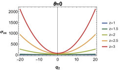
(a)

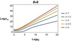
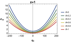
(b)

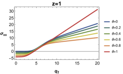
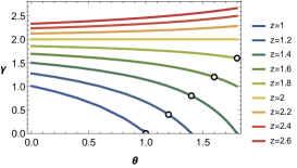
(c)

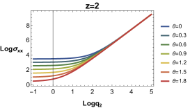
Figure 17: Scaling behavior of $\sigma_{xx}(q_{2})$ at large $q_{2}$ and $T=10$. (a) $z$-evolution of $\sigma_{xx}(q_{2})$ at $\theta=0$. (b) log-log plot of (a), (c) $\theta$-evolution of $\sigma_{xx}(q_{2})$ at $z=1$. (d) log-log plot of (c), (e) The exponent $\gamma$ of $\sigma_{xx}(q_{2})|_{q_{2}\rightarrow\infty}\sim q_{2}^{\gamma}$ for various $(z,\theta)$. Whenever $z=\theta$, the value of $\gamma$ is discontinuous, which is indicated by empty circles in the figure. At all the empty circle points, $\gamma=2$ which is discontinuous value from its neighboring point. Here, we analyzed this only in Phase A and B. (f) When $z=2$, $\gamma=2$ independent of $\theta$, which is indicated by yellow line in (e)

(a) $P_{0A}$ at $q_{\chi}=0$

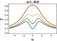
(b) $P_{0A}$ at $q_{\chi}=5$

(c) $P_{0B}$ at $q_{\chi}=0$

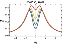
(d) $P_{0B}$

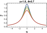
(e) $P_{A}$ at $q_{\chi}=0$

(f) $P_{A}$

(g) $P_{B}$ at $q_{\chi}=0$

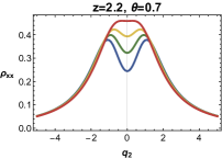
(h) $P_{B}$

(i) $P_{C}$ at $q_{\chi}=0$

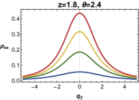
(j) $P_{C}$

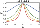
(k) $P_{D}$ at $q_{\chi}=0$

(l) $P_{D}$

Figure 18: Temperature evolution for $\rho_{xx}(q_{2})$ for various $(z,\theta)$. Curves correspond to $T=0.04,0.1,0.16,0.24$ for blue, green, yellow, and red respectively. In all figure, $q_{\chi}=5$ unless it is specified.

(a) $q_{\chi}=0$

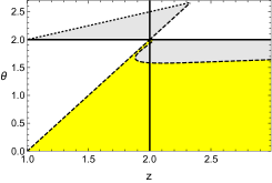
(b) $q_{\chi}=0.7$

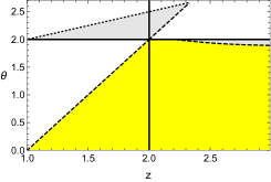
(c) $q_{\chi}=1.4$

Figure 19: WL vs WAL in the longitudinal resistivity. They are determined by the sign of the coefficient of $q_{2}^{2}$ near $q_{2}=0$. Yellow region denotes positive sign(WL) and gray region is for negative sign(WAL). Dotted line is NEC. Here we use the same parameters as Figure 18 and $T=0.04$.

Now we consider the density dependence of the longitudinal resistivity. Figure 18 shows the density dependence of $\rho_{xx}(q_{2})$. When $q_{2}=0$, the longitudinal resistivity is given by

$$\rho_{xx}|_{q_{2}=0}\equiv\rho_{xx}^{0}=\frac{r_{0}^{2z+\theta+2}}{r_{0}^{4z}+q_{\chi}^{2}\lambda^{4}r_{0}^{4\theta}}$$ (91)

where $r_{0}$ is $r_{H}(q_{2}=0)$. Different from electric conductivity, the resistivity does not have the scaling behavior in $T$, due to the $q_{\chi}^{2}$ term in denomenators.

For the finite density case, the relation between $r_{H}$ and $T$ is still complicated so we will take similar way to previous section. In the small $q_{2}$ limits, $q_{2}$ dependece of $r_{H}$ for fixed parameters $(T,\beta,\lambda,\theta,z)$ can be obtained from

$$\frac{\delta r_{H}}{\delta q_{2}}\bigg{|}_{q_{2}\ll 1} \sim-\frac{(z-\theta)^{2}r_{0}^{2\theta-1}}{z(z-\theta+2)(\theta-2)r_{0}^{2z}+(\theta-z)\beta^{2}r_{0}^{\theta}}q_{2}+\mathcal{O}(q_{2}^{4})$$

$$\equiv\mathcal{A}_{2}q_{2}+\mathcal{O}(q_{2}^{4})$$ (92)

Now, we have small $q_{2}$ expansion of $\rho_{xx}$ as

$$\rho_{xx}|_{q_{2}\ll 1} =\rho_{xx}^{0}-\frac{1}{\mathcal{D}^{2}}\bigg{(}\frac{2r_{0}^{2(3z+\theta)}-2q_{\chi}^{2}\lambda^{4}r_{0}^{2(z+3\theta)}}{\beta^{2}}$$

$$-\frac{\mathcal{A}_{2}}{2}r_{0}^{2z+\theta+1}\left(r_{0}^{4z}(2-2z+\theta)+q_{\chi}^{2}\lambda^{4}r_{0}^{4\theta}(2+2z-3\theta)\right)\bigg{)}q_{2}^{2}+\cdots$$ (93)

where $\mathcal{D}=r_{0}^{4z}+q_{\chi}^{2}\lambda^{4}r_{0}^{4\theta}$. The coefficient of $q_{2}^{2}$ in (B) determines a shape of the resistivity near $q_{2}=0$. Roughly speaking, $q_{\chi}$ can flip the sign of curvature flipped in $(z,\theta)$ dependent way, which is difficult to analyze. We calculated the the sign of the second term numerically and the result is in Figure 19. When $q_{\chi}=0$, the sign of coefficients of $q_{2}^{2}$ is always negative. In regions A,B, $q_{\chi}$ interaction suppress the resitivity near $q_{2}=0$, but the effect of $q_{\chi}$ diminishes as $\theta$ increases. In region C,D, the effect of $q_{\chi}$ terms become negligible due to the large $\theta$.

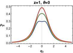
(a) $P_{0A}$

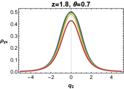
(b) $P_{A}$

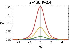
(c) $P_{C}$

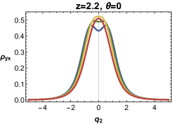
(d) $P_{0B}$

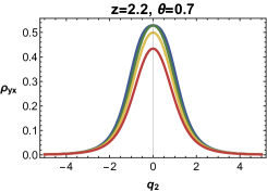
(e) $P_{B}$

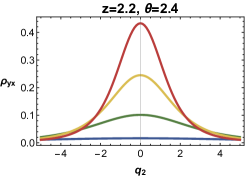
(f) $P_{D}$

Figure 20: Temperature evolution for $\rho_{yx}(q_{2})$ for different $(z,\theta)$. Each curves corresponds to $T=0.04,0.1,0.16,0.24$ for blue, green, yellow, and red respectively. In all figure, $q_{\chi}=5$.

Next, we consider the density dependence of the Hall conductivity. Figure 20 shows the density dependence of $\rho_{yx}(q_{2})$. When $q_{2}=0$, the longitudinal resistivity is given by

$$\rho_{yx}^{0}\equiv\rho_{yx}|_{q_{2}=0}=\frac{q_{\chi}\lambda^{4}r_{0}^{2+3\theta}}{r_{0}^{4z}+q_{\chi}^{2}\lambda^{4}r_{0}^{4\theta}},$$ (94)

where $r_{0}$ is $r_{H}(q_{2}=0)$. Also, we can expand $\rho_{yx}$ in small density limit as previous discussion,

$$\rho_{yx}(q_{2}) =\rho_{yx}^{0}-\frac{1}{2\mathcal{D}^{2}}\bigg{(}\frac{4q_{\chi}\lambda^{2}r_{0}^{4(z+\theta)}}{\beta^{2}}$$

$$+q_{\chi}\lambda^{2}r_{0}^{3\theta+1}\mathcal{A}_{2}\left(r_{0}^{4z}(4z-3\theta-2)+q_{\chi}^{2}\lambda^{4}r_{0}^{4\theta}(\theta-2)\right)\bigg{)}q_{2}^{2}+\cdots,$$ (95)

where $\mathcal{D}=(r_{0}^{4z}+q_{\chi}^{2}\lambda^{4}r_{0}^{4\theta})$.

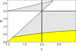
(a) $q_{\chi}=0.7$

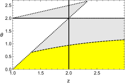
(b) $q_{\chi}=1.4$

Figure 21: Sign of the coefficient of $q_{2}^{2}$ of the transverse resistivity near $q_{2}=0$. Yellow region denotes positive sign(WL) and gray region is for negative sign(WAL). Dotted line is NEC. Here we use the same parameters as Figure 18 and $T=0.04$.

Roughly speaking, $q_{\chi}$ can flip the sign of curvature $(z,\theta)$ dependent way, which is difficult to analyze analytically. We investigated it numerically and the result is in Figure 21. In regions A, B, $q_{\chi}$-term suppress the resistivity near $q_{2}=0$, but the effect of $q_{\chi}$ is reduced as $\theta$ increases. In region C,D, the effect of $q_{\chi}$ terms becomes negligible due to the large $\theta$.

Now let’s turn to the density dependence of the thermal conductivity. We can perform the same analysis as the resistivity:

$$\kappa_{xx}(q_{2})=\kappa_{xx}^{0}-\frac{16\pi^{2}Tr_{0}^{2z-2\theta-1}}{\beta^{2}\mathcal{D}}\left(\frac{r_{0}^{4z+\theta+1}}{\beta^{2}}-(z-\theta)\mathcal{A}_{2}\mathcal{D}\right)q_{2}^{2}+\cdots,$$ (96)

$\mathcal{A}_{2}$ terms in (96) determines the curvature of the $\kappa_{xx}$ near the $q_{2}=0$. The sign of the coefficients is shown as Figure 23.

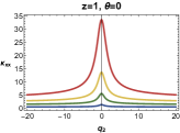
(a) $P_{0A}$ at $q_{\chi}=0$

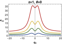
(b) $P_{0A}$

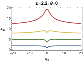
(c) $P_{0B}$ at $q_{\chi}=0$

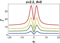
(d) $P_{0B}$

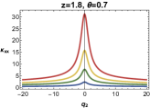
(e) $P_{A}$ at $q_{\chi}=0$

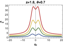
(f) $P_{A}$

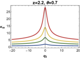
(g) $P_{B}$ at $q_{\chi}=0$

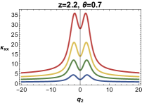
(h) $P_{B}$

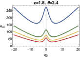
(i) $P_{C}$ at $q_{\chi}=0$

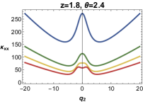
(j) $P_{C}$

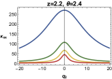
(k) $P_{D}$ at $q_{\chi}=0$

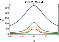
(l) $P_{D}$

Figure 22: Temperature evolution for $\kappa_{xx}(q_{2})$ for different $(z,\theta)$. Each curves corresponds to $T=0.04,0.1,0.160.24$ for blue, green, yellow, and red respectively. In all figure, $q_{\chi}=5$.

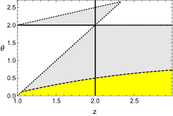
(a) $q_{\chi}=0.7$

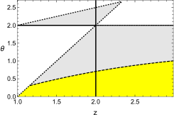
(b) $q_{\chi}=1.4$

Figure 23: Sign of the coefficient of $q_{2}^{2}$ of the $\kappa_{xx}$ near $q_{2}=0$. Yellow region denotes positive sign(WL) and gray region is for negative sign(WAL). Dotted line is NEC. Here we use the same parameters as Figure 22 and $T=0.04$.

Similarly, transverse thermal conductivity in small density limit is expressed as

$$\kappa_{xy}(q_{2})=\frac{16\pi^{2}Tq_{\chi}\lambda^{2}r_{0}^{\theta-2}}{\beta^{4}(1+q_{\chi}^{2}\lambda^{4}r_{0}^{-4(z-\theta)})}q_{2}^{2}+\cdots,$$ (97)

Notice that $\kappa_{xy}(q_{2}=0)=0$. The coefficient of $q_{2}^{2}$ in (97) is positive definite for every $(z,\theta)$. See Figure 24.

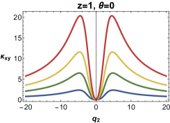
(a) $P_{0A}$

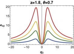
(b) $P_{A}$

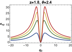
(c) $P_{C}$

(d) $P_{0B}$

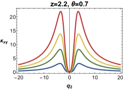
(e) $P_{B}$

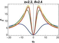
(f) $P_{D}$

Figure 24: Temperature evolution for $\kappa_{xy}(q_{2})$ for different $(z,\theta)$. Each curves corresponds to $T=0.04,0.1,0.16,0.24$ for blue, green, yellow, and red respectively. We used $q_{\chi}=5.$

Figure 25 and Figure 26 show the density dependence of Nernst signal and Seebeck coefficient respectively, which are related to the thermoelectric conductivity $\alpha$. We can expand $S(q_{2})$ and $N(q_{2})$ in the small density limit:

$$N \sim-\frac{4\pi q_{\chi}\lambda^{2}r_{0}^{2(z+\theta)}}{\beta^{2}\mathcal{D}}q_{2}+\cdots,$$

$$S \sim\frac{4\pi r_{0}^{4z}}{\beta^{2}\mathcal{D}}q_{2}+\cdots,$$ (98)

where $\mathcal{D}=r_{0}^{4z}+q_{\chi}^{2}\lambda^{4}r_{0}^{4\theta}$. The stepping feature near the zero $q_{2}$ in the figures 26 for nonzero $q_{\chi}$ case is due to the suppression of the linear term by the presence of $\cal D$ that contains $q_{\chi}^{2}$ which is chosen to be 5, which is rather large.

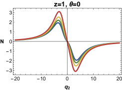
(a) $P_{0A}$

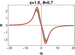
(b) $P_{A}$

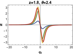
(c) $P_{C}$

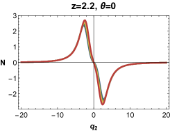
(d) $P_{0B}$

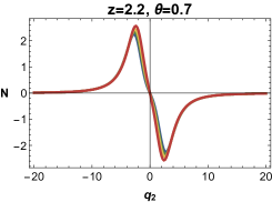
(e) $P_{B}$

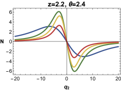
(f) $P_{D}$

Figure 25: Temperature evolution for $N(q_{2})$ for different $(z,\theta)$. Each curves corresponds to $T=0.04,0.1,0.16,0.24$ for blue, green, yellow, and red respectively. We used $q_{\chi}=5.$

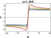
(a) $P_{0A}$ at $q_{\chi}=0$

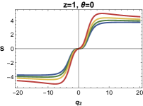
(b) $P_{0A}$

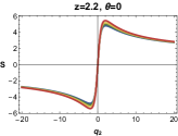
(c) $P_{0B}$ at $q_{\chi}=0$

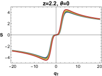
(d) $P_{0B}$

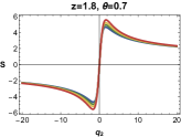
(e) $P_{A}$ at $q_{\chi}=0$

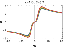
(f) $P_{A}$

(g) $P_{B}$ at $q_{\chi}=0$

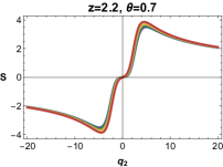
(h) $P_{B}$

(i) $P_{C}$ at $q_{\chi}=0$

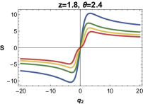
(j) $P_{C}$

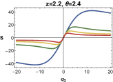
(k) $P_{D}$ at $q_{\chi}=0$

(l) $P_{D}$

Figure 26: Temperature evolution for $S(q_{2})$ for different $(z,\theta)$. Each curves corresponds to $T=0.04,0.1,0.160.24$ for blue, green, yellow, and red respectively. $q_{\chi}=5$ if $q_{\chi}\neq 0$.

Appendix C Null energy condition for Lifshitz black branes

The null energy condition (NEC) requires that, at every point in spacetime $T_{\mu\nu}v^{\mu}v^{\nu}\geq 0$, where $v^{\mu}$ is a light-like vector. $T_{\mu\nu}$ is the energy-momentum tensor of matter, suggesting that the NEC should be a property of matter. The NEC is used in deriving the second law of thermodynamics for black holes and in prohibiting the traversability of wormholes and the building of time machines. Einstein’s equations imply that the NEC can be reformulated in a form as

$$R_{\mu\nu}v^{\mu}v^{\nu}\geq 0,$$ (99)

However, the NEC can be violated by quantum fields. There are several examples of effective theories that violate NEC, but without manifest confliction with the principles of quantum field theory. At the quantum level, the NEC is violated by the Hawking effect. In this case, the quantum null energy condition is proposed as Bousso:2015wca

$$\langle T_{\nu\nu}\rangle\geq\frac{h}{2\pi}S^{\prime\prime},$$ (100)

where $S^{\prime\prime}$ is the local piece of the second null derivative of the entropy, evaluated on either side of the null surface.

The null energy condition for Lifshitz black branes with hyperscaling violating factors are $(z-1)(d+z-\theta)\geq 0$ and $(d-\theta)[d(z-1)-\theta]\geq 0$, where $d$ is the number of the spatial dimension.

The combination of the $tt$ and $rr$ components of Einstein equation is given by

$$R^{t}_{t}-R^{r}_{r}=\frac{1}{2}g^{rr}(\partial_{r}\phi)^{2}.$$ (101)

On the other hand, after evaluating the Ricci tensor for our ansatz, we obtain

$$R^{t}_{t}-R^{r}_{r}=-(2-\theta)(z-1-\frac{\theta}{2})r^{-\theta}f(r).$$ (102)

From (101) and (102), we obtain the solution for the dilaton field

$$e^{\phi}=r^{\sqrt{(2-\theta)(2z-2-\theta)}}.$$ (103)

To guarantee our black brane solution satisfies the Null energy condition, we require

$$\sqrt{(2-\theta)(2z-2-\theta)}\geq 0.$$ (104)

References

- (1) S. A. Hartnoll, A. Lucas and S. Sachdev, Holographic quantum matter, 1612.07324.
- (2) J. Zaanen, Y.-W. Sun, Y. Liu and K. Schalm, Holographic Duality in Condensed Matter Physics. Cambridge Univ. Press, 2015.
- (3) J. M. Maldacena, The Large N limit of superconformal field theories and supergravity, Int.J.Theor.Phys. 38 (1999) 1113–1133, [hep-th/9711200].
- (4) E. Witten, Anti-de Sitter space and holography, Adv. Theor. Math. Phys. 2 (1998) 253–291, [hep-th/9802150].
- (5) S. S. Gubser, I. R. Klebanov and A. M. Polyakov, Gauge theory correlators from noncritical string theory, Phys. Lett. B428 (1998) 105–114, [hep-th/9802109].
- (6) C. Charmousis, B. Gouteraux, B. S. Kim, E. Kiritsis and R. Meyer, Effective Holographic Theories for low-temperature condensed matter systems, JHEP 11 (2010) 151, [1005.4690].
- (7) B. Gouteraux and E. Kiritsis, Generalized Holographic Quantum Criticality at Finite Density, JHEP 12 (2011) 036, [1107.2116].
- (8) L. Huijse, S. Sachdev and B. Swingle, Hidden Fermi surfaces in compressible states of gauge-gravity duality, Phys. Rev. B85 (2012) 035121, [1112.0573].
- (9) N. Iizuka, S. Kachru, N. Kundu, P. Narayan, N. Sircar, S. P. Trivedi et al., Extremal Horizons with Reduced Symmetry: Hyperscaling Violation, Stripes, and a Classification for the Homogeneous Case, JHEP 03 (2013) 126, [1212.1948].
- (10) X. Dong, S. Harrison, S. Kachru, G. Torroba and H. Wang, Aspects of holography for theories with hyperscaling violation, JHEP 06 (2012) 041, [1201.1905].
- (11) K. Narayan, On Lifshitz scaling and hyperscaling violation in string theory, Phys. Rev. D85 (2012) 106006, [1202.5935].
- (12) E. Perlmutter, Hyperscaling violation from supergravity, JHEP 06 (2012) 165, [1205.0242].
- (13) M. Cadoni and S. Mignemi, Phase transition and hyperscaling violation for scalar Black Branes, JHEP 06 (2012) 056, [1205.0412].
- (14) M. Alishahiha and H. Yavartanoo, On Holography with Hyperscaling Violation, JHEP 11 (2012) 034, [1208.6197].
- (15) P. Dey and S. Roy, Lifshitz metric with hyperscaling violation from NS5-Dp states in string theory, Phys. Lett. B720 (2013) 419–423, [1209.1049].
- (16) M. Cadoni and M. Serra, Hyperscaling violation for scalar black branes in arbitrary dimensions, JHEP 11 (2012) 136, [1209.4484].
- (17) B. S. Kim, Hyperscaling violation : a unified frame for effective holographic theories, JHEP 11 (2012) 061, [1210.0540].
- (18) S. Kachru, X. Liu and M. Mulligan, Gravity duals of Lifshitz-like fixed points, Phys. Rev. D78 (2008) 106005, [0808.1725].
- (19) S.-J. Sin, S.-S. Xu and Y. Zhou, Holographic Superconductor for a Lifshitz fixed point, Int. J. Mod. Phys. A26 (2011) 4617–4631, [0909.4857].
- (20) S. A. Hartnoll and D. M. Hofman, Generalized Lifshitz-Kosevich scaling at quantum criticality from the holographic correspondence, Phys. Rev. B81 (2010) 155125, [0912.0008].
- (21) K. Goldstein, S. Kachru, S. Prakash and S. P. Trivedi, Holography of Charged Dilaton Black Holes, JHEP 08 (2010) 078, [0911.3586].
- (22) K. Goldstein, N. Iizuka, S. Kachru, S. Prakash, S. P. Trivedi and A. Westphal, Holography of Dyonic Dilaton Black Branes, JHEP 10 (2010) 027, [1007.2490].
- (23) V. Keranen and L. Thorlacius, Thermal Correlators in Holographic Models with Lifshitz scaling, Class. Quant. Grav. 29 (2012) 194009, [1204.0360].
- (24) Z. Zhao, Q. Pan and J. Jing, Notes on analytical study of holographic superconductors with Lifshitz scaling in external magnetic field, Phys. Lett. B735 (2014) 438–444, [1311.6260].
- (25) J.-W. Lu, Y.-B. Wu, P. Qian, Y.-Y. Zhao and X. Zhang, Lifshitz Scaling Effects on Holographic Superconductors, Nucl. Phys. B887 (2014) 112–135, [1311.2699].
- (26) Y. Bu, Holographic superconductors with Lifshitz scaling, Phys. Rev. D86 (2012) 046007, [1211.0037].
- (27) E. J. Brynjolfsson, U. H. Danielsson, L. Thorlacius and T. Zingg, Holographic Superconductors with Lifshitz Scaling, J. Phys. A43 (2010) 065401, [0908.2611].
- (28) S. Harrison, S. Kachru and H. Wang, Resolving Lifshitz Horizons, JHEP 02 (2014) 085, [1202.6635].
- (29) A. Donos and J. P. Gauntlett, Novel metals and insulators from holography, JHEP 06 (2014) 007, [1401.5077].
- (30) M. Blake, A. Donos and N. Lohitsiri, Magnetothermoelectric Response from Holography, JHEP 08 (2015) 124, [1502.03789].
- (31) R. A. Davison and B. Goutéraux, Momentum dissipation and effective theories of coherent and incoherent transport, JHEP 01 (2015) 039, [1411.1062].
- (32) B. Goutéraux, Charge transport in holography with momentum dissipation, JHEP 04 (2014) 181, [1401.5436].
- (33) D. Giataganas and K. Sfetsos, Non-integrability in non-relativistic theories, JHEP 06 (2014) 018, [1403.2703].
- (34) P. Fonda, L. Franti, V. Keränen, E. Keski-Vakkuri, L. Thorlacius and E. Tonni, Holographic thermalization with Lifshitz scaling and hyperscaling violation, JHEP 08 (2014) 051, [1401.6088].
- (35) I. Papadimitriou, Hyperscaling violating Lifshitz holography, Nucl. Part. Phys. Proc. 273-275 (2016) 1487–1493, [1411.0312].
- (36) M. H. Dehghani, A. Sheykhi and S. E. Sadati, Thermodynamics of nonlinear charged Lifshitz black branes with hyperscaling violation, Phys. Rev. D91 (2015) 124073, [1505.01134].
- (37) H.-S. Liu, H. Lu and C. N. Pope, Magnetically-Charged Black Branes and Viscosity/Entropy Ratios, JHEP 12 (2016) 097, [1602.07712].
- (38) X.-H. Ge, Y. Tian, S.-Y. Wu and S.-F. Wu, Hyperscaling violating black hole solutions and Magneto-thermoelectric DC conductivities in holography, Phys. Rev. D96 (2017) 046015, [1606.05959].
- (39) X.-H. Ge, S.-J. Sin, Y. Tian, S.-F. Wu and S.-Y. Wu, Charged BTZ-like black hole solutions and the diffusivity-butterfly velocity relation, JHEP 01 (2018) 068, [1712.00705].
- (40) Z.-N. Chen, X.-H. Ge, S.-Y. Wu, G.-H. Yang and H.-S. Zhang, Magnetothermoelectric DC conductivities from holography models with hyperscaling factor in Lifshitz spacetime, Nucl. Phys. B924 (2017) 387–405, [1709.08428].
- (41) S. Cremonini, M. Cvetic and I. Papadimitriou, Thermoelectric DC conductivities in hyperscaling violating Lifshitz theories, JHEP 04 (2018) 099, [1801.04284].
- (42) S. Mukhopadhyay and C. Paul, Hyperscaling violating geometry with magnetic field and DC conductivity, Nucl. Phys. B938 (2019) 571–593, [1906.02348].
- (43) Y. Ahn, H.-S. Jeong, D. Ahn and K.-Y. Kim, Linear- Resistivity from Low to High Temperature: holographic Q-lattice model, 1907.12168.
- (44) Y. Seo, G. Song, C. Park and S.-J. Sin, Small Fermi Surfaces and Strong Correlation Effects in Dirac Materials with Holography, JHEP 10 (2017) 204, [1708.02257].
- (45) Y. Seo, G. Song and S.-J. Sin, Strong Correlation Effects on Surfaces of Topological Insulators via Holography, Phys. Rev. B96 (2017) 041104, [1703.07361].
- (46) M. Liu, J. Zhang, C.-Z. Chang, Z. Zhang, X. Feng, K. Li et al., Crossover between weak antilocalization and weak localization in a magnetically doped topological insulator, Phys. Rev. Lett. 108 (2012) 036805.
- (47) D. Zhang et al., Interplay between ferromagnetism, surface states, and quantum corrections in a magnetically doped topological insulator, Physical Review B 86 (2012) 205127.
- (48) L. Bao, W. Wang, N. Meyer, Y. Liu, C. Zhang, K. Wang et al., Quantum corrections crossover and ferromagnetism in magnetic topological insulators, Scientific reports 3 (2013) .
- (49) J. Crossno, J. K. Shi, K. Wang, X. Liu, A. Harzheim, A. Lucas et al., Observation of the Dirac fluid and the breakdown of the Wiedemann-Franz law in graphene, Science 351 (Mar., 2016) 1058–1061, [1509.04713].
- (50) A. Lucas, J. Crossno, K. C. Fong, P. Kim and S. Sachdev, Transport in inhomogeneous quantum critical fluids and in the Dirac fluid in graphene, Phys. Rev. B93 (2016) 075426, [1510.01738].
- (51) Y. Seo, G. Song, P. Kim, S. Sachdev and S.-J. Sin, Holography of the Dirac Fluid in Graphene with two currents, Phys. Rev. Lett. 118 (2017) 036601, [1609.03582].
- (52) Y. Seo, K.-Y. Kim, K. K. Kim and S.-J. Sin, Character of matter in holography: Spin–orbit interaction, Phys. Lett. B759 (2016) 104–109, [1512.08916].
- (53) E. D. L. Rienks, S. Wimmer, J. Sánchez-Barriga, O. Caha, P. S. Mandal, J. Růžička et al., Large magnetic gap at the Dirac point in Bi2Te3/MnBi2Te4 heterostructures, Nature 576 (2019) 423–428.
- (54) H. Min, R. Bistritzer, J.-J. Su and A. H. MacDonald, Room-temperature superfluidity in graphene bilayers, Phys. Rev. B 78 (Sep, 2008) 121401.
- (55) A. Donos and J. P. Gauntlett, Thermoelectric DC conductivities from black hole horizons, JHEP 1411 (2014) 081, [1406.4742].
- (56) R. Bousso, Z. Fisher, J. Koeller, S. Leichenauer and A. C. Wall, Proof of the Quantum Null Energy Condition, Phys. Rev. D93 (2016) 024017, [1509.02542].