Focused Bayesian Prediction

Abstract

We propose a new method for conducting Bayesian prediction that delivers accurate predictions without correctly specifying the unknown true data generating process. A prior is defined over a class of plausible predictive models. After observing data, we update the prior to a posterior over these models, via a criterion that captures a user-specified measure of predictive accuracy. Under regularity, this update yields posterior concentration onto the element of the predictive class that maximizes the expectation of the accuracy measure. In a series of simulation experiments and empirical examples we find notable gains in predictive accuracy relative to conventional likelihood-based prediction.

Keywords: Loss-based Bayesian forecasting; proper scoring rules; stochastic volatility; expected shortfall; Murphy diagram; M4 forecasting competition

MSC2010 Subject Classification: 62F15, 60G25, 62M20

JEL Classifications: C11, C53, C58.

1 Introduction

Bayesian prediction quantifies uncertainty about the future value of a random variable using the rules and language of probability. A probability distribution for a future value is produced, conditioned only on past observations; all uncertainty about the parameters of the prediction model, plus any uncertainty about the model itself, having been integrated, or averaged out via these simple rules. Inherent to this natural and coherent approach to prediction, however, is the assumption that the process that has generated the observed data is either equivalent to the particular model on which we condition, or contained in the set of models over which we average. Such a heroic assumption is clearly at odds with reality; in particular in the realm of the social and economic sciences where statistical data arises through complex processes that we can only ever intend to approximate.

In response to this limitation of the conventional paradigm, we propose an alternative approach to Bayesian prediction. A prior is placed over a class of plausible predictive models. The prior is then updated to a posterior over these models, via a criterion function that represents a user-specified measure of predictive accuracy. This criterion replaces the likelihood function in the conventional Bayesian update and, hence, obviates the explicit need for correct model specification. Summarization of the posterior so produced - via its mean, for example - yields a single, representative predictive distribution that is expressly designed to yield accurate forecasts according to the given measure. Alternatively, the full extent of the posterior variation that obtains can be quantified and visualized. Given this deliberate focus on a particular aspect of predictive performance in the building of predictions, we refer to the principle as focused Bayesian prediction, or simply FBP.

To quantify predictive accuracy we use the concept of a scoring rule. (See Gneiting et al.,, 2007, and Gneiting and Raftery,, 2007, for early expositions.) In short, a scoring rule rewards a probabilistic forecast for assigning a high density ordinate (or high probability mass) to the observed value (‘calibration’), subject to some criterion of ‘sharpness’, or some reward for accuracy in a particular part of the predictive support (e.g. the tails; Diks et al.,, 2011, Opschoor et al.,, 2017). Under appropriate regularity, we establish that this approach ensures, asymptotically, accurate performance according to the specified measure of predictive accuracy, and without dependence on correct model choice. Extensive numerical results support the theoretical results: focus on predictive accuracy, rather than correct model specification per se, leads to improved predictive performance.

This approach to Bayesian prediction has elements in common with the ‘probably approximately correct’ (PAC)-Bayes approach to prediction adopted in the machine learning literature; see Guedj, (2019) for a recent review and extensive referencing. The use of Bayesian updating per se without reference to a likelihood function also echoes the generalized inferential methods proposed by, for example, Bissiri et al., (2016), Giummolè et al., (2017), Knoblauch et al., (2019) and Syring and Martin, (2019), in which uncertainty about unknown parameters (in a given model) is updated via a general loss, or score, function. A major challenge in these generalizations of the standard Bayesian paradigm is the calibration of the scale of the loss (or score), which has a direct impact on the resultant variance of posterior of the parameters. Several methods for specifying this scale have been proposed (Bissiri et al.,; Giummolè et al.,; Holmes and Walker,, 2017; Lyddon et al.,, 2019; Syring and Martin,). Whilst we draw some insights from this literature, we propose new approaches that are informed specifically by the prediction context in which we are working, and which ensure posterior concentration around the predictive that is optimal under the given accuracy measure.

The predictive distributions within the plausible class may characterize a single dynamic structure depending on a single vector of unknown parameters. However, they may also be weighted combinations of predictives from distinct models. As such, our approach represents a coherent Bayesian method for estimating weighted combinations of predictives via forecast accuracy criteria, and without the need to assume that the true model lies within the set of constituent predictives. Whilst an established literature on estimating mixtures of predictives exists (see Aastveit et al.,, 2019, for an extensive review) - including work that invokes Bayesian principles - our paper provides an alternative way of updating predictive combinations via non-likelihood-based Bayesian principles. We comment further on the connection of our work with the literature on predictive combinations, plus provide detailed referencing to this literature, in Section 4.2.

After establishing the theoretical validity of the new method, its efficacy and usefulness is demonstrated through a set of simulation exercises, based on alternative predictive classes for a stochastic volatility model for financial returns. These classes are deliberately chosen to represent, at one end, a very misspecified representation of the (known) true data generating process (DGP) and, at the other end, a less misspecified version. The comparator in all cases is the standard, and misspecified, likelihood-based Bayesian update of the given parametric class. The results are clear: within-sample updating based on a specific measure of predictive accuracy almost always leads to the best out-of-sample performance according to that measure. The degree of superiority depends on the interplay between the model class, including the manner in which the model is misspecified, and the desired measure of accuracy - with animated graphics used to illustrate this point. The differential impact of update choice on posterior variation is also highlighted, via an animated display of posterior distributions for the expected shortfall (ES) of both ‘long’ and ‘short’ portfolios in the financial asset.

Two empirical illustrations complete the analysis. In the first, we predict two different series of daily financial returns using predictive classes based on the Gaussian (generalized) autoregressive conditional heteroscedastic ((G)ARCH) class of volatility model, known to be misspecified for the more complex process driving returns. The series considered are returns on: the U.S. dollar currency index, and the S&P500 stock index. The empirical results mimic those produced by simulation, with predictive accuracy improved by using the focused update - rather than the conventional (likelihood-based) update - in virtually all cases. The increase in predictive accuracy translates into more accurate value at risk (VaR) forecasts: use of an update that focuses on tail accuracy leads to a better match of empirical to nominal VaR coverage (than does the likelihood update) in all cases, and more frequent support of the joint null of correct coverage and independent violations. Improved forecasts of ES also result in many cases.

In the second empirical example we pit FBP against the best performers in the Makridakis 4 (M4) forecasting competition. We perform the exercise using the 23,000 annual time series from the set of 100,000 series (of varying frequencies) used in the competition. We select as the predictive class, the exponential smoothing model of Hyndman et al., (2002) (referred to as ETS hereafter), which had ranked highly amongst all twenty-five competitors. Adopting the same preliminary model selection procedure as the authors to specify the components of the ETS class for each of the 23,000 series, we update the chosen class using the mean scaled interval score (MSIS). This measure of predictive accuracy penalizes a prediction interval if the observed value falls outside the interval (appropriately weighted by its nominal coverage), and rewards a narrow interval, and was one of the measures used to rank methods in the competition. As measured by MSIS, FBP not only almost always outperforms maximum likelihood-based implementation of ETS, but it outperforms all four predictive methods that were previously ranked best in the competition, in a large number of cases.

The rest of the article is organized as follows. In Section 2 we propose our new Bayesian predictive paradigm, and briefly illustrate its ability to produce more accurate predictions using a toy example. In Section 3 asymptotic validation of the method is provided, under the required regularity. More extensive illustration of the new approach via simulation, and visualization of the results, is the content of Section 4, whilst Section 5 illustrates the power of the method in empirical settings. In Section 6 we discuss the implications of our results and future lines of research. The proofs of all theoretical results, and certain computational details, are provided in appendices to the paper.

2 Focused Bayesian Prediction

2.1 Preliminaries and notation

Consider a stochastic process $\{y_{t}:\Omega\rightarrow\mathbb{R},t\in\mathbb{N}\}$ defined on the complete probability space $(\Omega,\mathcal{F},G)$. Let $\mathcal{F}_{t}:=\sigma(y_{1},\dots,y_{t})$ denote the natural sigma-field, and let $G$ denote the infinite-dimensional distribution of the sequence $y_{1},y_{2},\dots$.

Throughout, we focus on one-step-ahead predictions and let $\mathcal{P}^{t}:=\left\{P_{\bm{\theta}}^{t}:\bm{\theta}\in\Theta\right\}$ denote a generic class of one-step-ahead predictive models for $y_{t+1}$, which are conditioned on time $t$ information $\mathcal{F}_{t}$, and where the generic elements of $\mathcal{P}^{t}$ are represented by $P_{\bm{\theta}}^{t}(\cdot):=P(\cdot|\bm{\theta},\mathcal{F}_{t}).$ The  parameter $\bm{\theta}$ indexes values in the predictive class, with $\bm{\theta}$ defined on $(\Theta,\mathcal{T},\Pi)$, and where $\Pi$ measures our beliefs about $\bm{\theta}$. Our beliefs $\Pi$ over $\Theta$ - both prior and posterior - generate corresponding beliefs over the elements in the predictive class $\mathcal{P}^{t}$, in the usual manner and, therefore, throughout the remainder we abuse notation and refer to $\Pi$ as indexing beliefs over the class $\mathcal{P}^{t}$.

Our goal is to construct a sequence of probability measures over $\mathcal{P}^{t}$, starting from our prior beliefs $\Pi$, such that hypotheses in $\mathcal{P}^{t}$ that have ‘higher predictive accuracy’, are given higher posterior probability, after observing realizations from $\{y_{t}:t\geq 1\}$. Given a user-defined measure of accuracy, we demonstrate that such a probability measure can be constructed using a Bayesian updating framework.

Importantly however, we deviate from the standard approach to the production of Bayesian predictives in that the class $\mathcal{P}^{t}$ only represents plausible predictive models for $y_{t+1}$. At no point in what follows do we make the unrealistic assumption that the true one-step-ahead predictive is contained in $\mathcal{P}^{t}$.

2.2 Bayesian updating based on scoring rules

Using generic notation for the moment, for $\mathcal{P}$ a convex class of predictive distributions on $(\Omega,\mathcal{F})$, we measure the predictive accuracy of $P\in\mathcal{P}$ using the scoring rule $S:\mathcal{P}\times\Omega\rightarrow\mathbb{R}$, whereby if the predictive distribution $P$ is quoted and the value $y$ eventuates, then the reward, or positively-oriented ‘score’, is $S(P,y).$ The expected score under the true predictive $G$ is defined as

$$\mathbb{S}(\cdot,G):=\int_{y\in\Omega}S(\cdot,y)dG(y).$$ (1)

We say that a scoring rule is proper relative to $\mathcal{P}$ if, for all $P,G\in\mathcal{P}$, $\mathbb{S}(G,G)\geq\mathbb{S}(P,G),$ and is strictly proper, relative to $\mathcal{P}$, if $\mathbb{S}(G,G)=\mathbb{S}(P,G)\iff P=G.$ That is, a proper scoring rule is one whereby if the forecaster’s best judgment is indeed the true measure $G$ there is no incentive to quote anything other than $P=G$ (Gneiting and Raftery,, 2007).

Under the assumption that a given predictive class contains the truth, i.e. that $G\in\mathcal{P}$, the expectation of any proper score $S(\cdot,y)$, with respect to the truth $(G)$, will be maximized at the truth, $G$. Hence, maximization over $\mathcal{P}$ of the expected scoring rule $\mathbb{S}(\cdot,G)$, will reveal the true predictive mechanism when it is contained in $\mathcal{P}$. In practice of course, the expected score $\mathbb{S}(\cdot,G)$ is unattainable, and a sample estimate based on observed data is used to define a sample score-based criterion. Maximization of the sample criterion, which implicitly depends on the true predictive process through the observed data, will yield the member of the predictive class that maximizes the relevant sample criterion. However, asymptotically the true predictive distribution will be recovered via any proper score criterion (again, on the assumption that the true predictive lies in the class $\mathcal{P}$).

The very premise of this paper is that, in reality, any choice of predictive class is such that the truth is not contained therein, at which point there is no reason to presume that the expectation of any particular scoring rule will be maximized at the truth or, indeed, maximized by the same predictive distribution that maximizes a different (expected) score. This does not, however, preclude the meaningfulness of a score as a measure of predictive accuracy, or invalidate the goal of seeking accuracy according to this particular measure. Indeed, it renders the distinctiveness of different scoring rules, and what form of forecast accuracy they do and do not reward, even more critical, and provides strong justification for driving predictive decisions by the very score that matters for the problem at hand.

With these insights in mind, we proceed as follows, reverting now to the specific notation that characterizes our problem, as defined in Section 2.1. Given observed data $\mathbf{y}_{n}=(y_{1},y_{2},...,y_{n})^{\prime}$, our object of interest is $P_{\bm{\theta}}^{n}$, that is, the predictive distribution for $y_{n+1}$, conditional on information known at time $n$, $\mathcal{F}_{n}$. Given our prior beliefs $\Pi(\cdot)$, over $\mathcal{P}^{n}$, we update these beliefs using the following coherent posterior measure: for $A\subset\mathcal{P}^{n}$,

$$\Pi_{w}(A|\mathbf{y}_{n})=\frac{\int_{A}\exp\left[w_{n}S_{n}\left(P_{\bm{\theta}}^{n}\right)\right]\text{d}\Pi\left(P_{\bm{\theta}}^{n}\right)}{\int_{\Theta}\exp\left[w_{n}S_{n}\left(P_{\bm{\theta}}^{n}\right)\right]\text{d}\Pi\left(P_{\bm{\theta}}^{n}\right)},$$ (2)

where

$$S_{n}(P_{\bm{\theta}}^{n})=\sum\limits_{t=0}^{n-1}S(P_{\bm{\theta}}^{t},y_{t+1}),$$ (3)

and where the scale factor $w_{n}$ (indexed by $n$), used to define and index the posterior (via the notation $\Pi_{w}(\cdot|\mathbf{y}_{n})$), is to be discussed in detail below. Two more comments regarding notation are useful at this point. First, consistent with our earlier comment, we abuse notation by defining a prior directly over a predictive, $P_{\bm{\theta}}^{n}$ here. In fact, the prior is placed over $\bm{\theta}$, and the prior over $P_{\bm{\theta}}^{n}$ merely implied. Hence, the incongruous appearance of conditioning data in the prior (through the definition of $P_{\bm{\theta}}^{n}$) is of no concern. It is simply used to define the particular function of $\bm{\theta}$ ($P_{\bm{\theta}}^{n}$) that is our ultimate object of interest, and that function conditions on (past) observed data, as it is a predictive distribution. Second, the criterion function that defines the update in (2) is, of course, comprised of the sequential one-step-ahead predictives, $P_{\bm{\theta}}^{t},$ for $t=0,1,...,n-1.$

The use of the non-likelihood-based update in (2) mimics various generalizations of the standard Bayesian inferential paradigm that have been proposed. Such generalizations replace the likelihood with the exponential of a problem-specific loss function; the goal being to produce useful inference in the realistic setting in which the true DGP is unknown, and the correct likelihood function thus unavailable. This literature has its roots in the ‘Gibbs posteriors’ of Zhang, 2006a , Zhang, 2006b and Jiang and Tanner, (2008), in which the exponential of a general loss function replaces the likelihood function in the Bayesian update. However, it is arguably Bissiri et al., (2016), and the subsequent related work in (inter alia) Holmes and Walker, (2017), Lyddon et al., (2019) and Syring and Martin, (2019), that have given the method its recent prominence in the statistics and econometrics literature.

The PAC-Bayes algorithms used in machine learning are also characterized, in part, by exponential functions of general losses. The focus therein is on loss defined with respect to predictors, rather than parameters; hence the particular connection with our approach. Our work is, however, quite distinct from PAC-Bayes. Most notably, the updating mechanism in (2) is expressed in terms of a class of plausible conditional predictive distributions, rather than point predictors, and the ‘loss function’ defined explicitly in terms of a proper scoring rule. We also entertain predictive models that feature in the statistics and/or econometrics literature, and provide asymptotic validation of the method in this context.

The update in (2) is coherent in the sense that the posterior that results from updating the prior using two sets of observations in one step, is the same as that produced by two sequential updates. Proof of this property follows that of Bissiri et al., (2016) and exploits the exponential form of the first term on the right-hand-side of (2), in addition to certain conditions on $w_{n}$ to be made explicit below. Indeed, the appearance of $w_{n}$ serves to distinguish (2) from what would be an extension (to the predictive setting) of the loss-based inference approach adopted by Chernozhukov and Hong, (2003).

In the case where $w_{n}=1$ and $S(P_{\bm{\theta}}^{t},y_{t+1})=\ln p\left(y_{t+1}|\mathcal{F}_{t},\bm{\theta}\right),$ with $p\left(y_{t+1}|\mathcal{F}_{t},\bm{\theta}\right)$ denoting the predictive density (or mass) function associated with the class $\mathcal{P}^{t}$, the update in (2) obviously defaults to the conventional likelihood-based update of the prior defined over $\bm{\theta}$. We refer hereafter to this special case as ‘exact Bayes’, and acknowledge that, given the presumption of misspecification, there is no sense in which exact Bayes remains the ‘gold standard’. This case remains, however, a critical benchmark in the numerical work,  in which the degree of misspecification of $\mathcal{P}^{t}$ will be seen to influence the relative out-of-sample performance of the conventional Bayesian update.

We can summarize the posterior in (2) by producing a simulation-based estimate of the mean predictive:

$$\mathbb{E}_{w}\left[P_{\bm{\theta}}^{n}|\mathbf{y}_{n}\right]=\int P_{\bm{\theta}}^{n}\text{d}\Pi_{w}(P_{\bm{\theta}}^{n}|\mathbf{y}_{n}).$$ (4)

However, it is equally feasible to construct measures that capture the variability of the posterior, such as quantiles or the posterior variance. Moreover, we can use various graphical techniques to visualize the variation of the predictives themselves and understand the way in which posterior variation over the class $\mathcal{P}^{t}$ impacts on predictive accuracy per se.

Before moving on, we quickly demonstrate the usefulness of this new approach to Bayesian prediction, and the predictive gains that it can reap, using a simple toy example.

2.3 A toy example: ARCH(1)

We produce predictive distributions for a financial return generated from a latent stochastic volatility model with a skewed marginal distribution, with precise details of this true DGP to be given in Section 4. The predictive class, $\mathcal{P}^{t}$, is defined by an ARCH model of order 1 (ARCH(1)) with Gaussian errors, $y_{t}=\theta_{1}+\sigma_{t}{\epsilon_{t},}$ ${\epsilon_{t}\sim i.i.d.N\left(0,1\right),}$ ${\sigma_{t}^{2}}{=\theta_{2}+\theta_{3}\left(y_{t-1}-\theta_{1}\right)^{2},}$ with $\bm{\theta}=\left(\theta_{1},\theta_{2},\theta_{3}\right)^{\prime}$, and $\pi\left(\bm{\theta}\right)\propto\frac{1}{\theta_{2}}\times I\left[\theta_{2}>0,\theta_{3}\in[{0,1)}\right]]$ (with $I$ the indicator function) defining a prior density over $\bm{\theta}$.

For $p\left(y_{t+1}|\mathcal{F}_{t},\bm{\theta}\right)$ denoting the predictive density function associated with the Gaussian ARCH(1) class, we implement FBP using the following two scoring rules:

$$S_{\text{LS}}(P_{\bm{\theta}}^{t},y_{t+1}) =\ln p\left(y_{t+1}|\mathcal{F}_{t},\bm{\theta}\right)$$ (5)

$$S_{\text{CS}}(P_{\bm{\theta}}^{t},y_{t+1}) =\ln p\left(y_{t+1}|\mathcal{F}_{t},\bm{\theta}\right)I\left(y_{t+1}\in A\right)+\left[\ln\int_{A^{c}}p\left(y|\mathcal{F}_{t},\bm{\theta}\right)dy\right]I\left(y_{t+1}\in A^{c}\right).$$ (6)

As noted already, use of the log score (LS), (5), in (2) (with $w_{n}=1$) yields the conventional likelihood-based Bayesian update, and we label the results based on this score as exact Bayes as a consequence. The score in (6) is the censored likelihood score (CS) introduced by Diks et al., (2011), and applied by Opschoor et al., (2017) to the prediction of financial returns. This score rewards predictive accuracy over the region of interest $A$ (with $A^{c}$ indicating the complement of this region). Here we report results solely for $A$ defining the lower and upper tail of the predictive distribution, as determined respectively by the 10% and 90% quantile of the empirical distribution of $y_{t}$. We label the results based on the use of (6) in (2) (also using $w_{n}=1$) as FBP-CS_<10% and FBP-CS${}_{>90\%}.$

Postponing discussion of the full design details until Section 4, we record in Table 1 out-of-sample results based on repeated computation of (4) using expanding windows to produce (via Markov chain Monte Carlo) draws from (2). Using a total of 2,000 out-of-sample values, the average LS (computed across the 2,000 mean predictives) and the average CS for the lower and upper 10% tail (denoted by CS_<10% and CS_>90% respectively) are computed for each of the three different updating methods. Recalling that we use positively-oriented scores, the largest average score, according to each out-of-sample evaluation method, is highlighted in bold.

		Out-of-sample score
		LS	CS<10%	CS>90%
Updating method
Exact Bayes		-1.3605	-0.4089	-0.2745
FBP-CS<10%		-1.4420	-0.3943	-0.3833
FBP-CS>90%		-3.0067	-1.4157	-0.2397

Table 1: Predictive accuracy of FBP, using the ARCH(1) predictive class. The rows in each panel refer to the update method used. The columns refer to the out-of-sample measure used to compute the average scores. The figures in bold are the largest average scores according to a given out-of-sample measure.

We see that use of the CS rule in the posterior update yields better out-of-sample performance, as measured by that score, in both the upper and lower tails. In absolute terms, the gain of ‘focusing’ is more substantial in the upper tail than the lower tail, and in Section 4 we shall see why this is so. The average LS produced by the exact Bayes (LS-based) update is also larger than the average LS produced by both FBP-CS_<10% and FBP-CS_>90%.

In summary, focusing works, and the following theoretical results give some insight into why.

3 Bayesian and Frequentist Agreement

Whilst the elements of $\mathcal{P}^{t}$ may, in principle, be either parametric or nonparametric conditional distributions, in the remainder we focus on the parametric case to simplify the analysis, leaving rigorous analysis of nonparametric conditionals for later study. However, we remind the reader that this reduction to parametric conditionals covers both the canonical case where the elements of $\mathcal{P}^{t}$ are indexed by a finite-dimensional parameter, in which case $\Theta$ is a Euclidean space, as well as the case where the elements in $\mathcal{P}^{t}$ are (a finite collection of) mixtures of predictives, in which case $\Theta$ denotes either the weights of the mixture, or the combination of the weights and the unknown parameters of the constituent predictives.

3.1 Choosing $w_{n}$

With reference to the conventional Bayesian approach to inference on the unknown parameters, $\bm{\theta}$, which characterize an assumed DGP, the posterior density,

$$\pi(\bm{\theta}|\mathbf{y}_{n})\propto\ell(\mathbf{y}_{n}|\bm{\theta})\pi(\bm{\theta}),$$ (7)

where $\ell(\mathbf{y}_{n}|\bm{\theta})$ denotes the likelihood function, arises via a decomposition of the joint probability distribution for $\bm{\theta}$ and the random vector $\mathbf{y}_{n}.$ As such, the representation of $\pi(\bm{\theta}|\mathbf{y}_{n})$ as proportional to the product of a density (or mass) function for $\mathbf{y}_{n}$, and the prior for $\bm{\theta}$, reflects the usual calculus of probability distributions, and provides a natural ‘weighting’ between the likelihood and the prior.

Once one moves away from this conventional framework, and replaces the likelihood with an alternative mechanism through which the data provides information about $\bm{\theta}$, this natural weighting is lost. Instead, a subjective choice must be made regarding the relative weight given to prior and data-based information in the production of the posterior, with the scale factor $w_{n}$ in (2) denoting this subjective choice of weighting. Bissiri et al., (2016) propose several methods for choosing $w_{n}$, including annealing methods, hyper-parametrization of $w_{n}$, and setting $w_{n}$ to ensure the equivalence of the expected ‘loss’ of the prior and data-based components of (2). The authors also suggest choosing $w_{n}$ to ensure correct frequentist coverage of posterior credible intervals, plus the use of priors that are conjugate to the weighted data-based criterion.

In contrast, our interest is not in inference on $\bm{\theta}$ per se, but in forecast accuracy. Given this goal, from a theoretical standpoint, our only concern is that, for $\{w_{n}:n\geq 1\}$ a chosen scaling sequence, the FBP posterior measure concentrates onto the element of $\mathcal{P}^{n}$ that is most accurate in the chosen scoring rule, which is defined by the following value in $\Theta$:

$$\bm{\theta}_{\ast}=\operatorname*{arg\,max}_{\bm{\theta}\in\Theta}\lim_{n\rightarrow\infty}\mathbb{E}\left[{S}_{n}(P_{\bm{\theta}}^{n})/n\right].$$ (8)

As the following result demonstrates, this concentration occurs for any reasonable choice of $w_{n}$.

Lemma 1.

Assume Assumptions 1-3 in Appendix A are satisfied, and denote the FBP posterior density function by $\pi_{w}\left(\bm{\theta}|\mathbf{y}_{n}\right)$. If the sequence $\{w_{n}\}$ satisfies $\lim_{n}w_{n}=C$, $0<C<\infty$, the posterior density $\pi_{w}(\cdot|\mathbf{y}_{n})$ converges to $P_{\bm{\theta}_{\ast}}:=\lim_{n\rightarrow\infty}P_{\bm{\theta}_{\ast}}^{n},$ the limit of the predictive defined by $\bm{\theta}_{\ast}$, at rate $1/\sqrt{n}$.

Remark 1.

The above result demonstrates that, if we restrict our analysis to a class of parametric predictives, FBP asymptotically concentrates, at rate $1/\sqrt{n}$, onto the predictive that is most accurate according to the scoring rule $P_{\bm{\theta}}^{t}\mapsto\lim_{n}\mathbb{E}\left[S(P_{\bm{\theta}}^{t},\cdot)/n\right]$.

Remark 2.

The conditions for the above result are discussed in Appendix A and are similar to the standard regularity conditions for parametric $M$-estimators, along with some uniform control on the tail of the prior $\Pi$. These conditions are similar to those used elsewhere in the literature, e.g., Chernozhukov and Hong, (2003). Interestingly, Lemma 1 is valid for a wide variety of $\{w_{n}\}$. In Sections 4 and 5, we detail the particular values of $w_{n}$ that we use to produce our numerical predictions.

3.2 Merging

In the previous section, we have seen that, for a reasonable choice of $w_{n}$, the FBP posterior concentrates on the element of $\mathcal{P}^{n}$ that is most accurate for prediction under the chosen scoring rule. In this section, we compare the behavior of predictions obtained from the FBP posterior with those that would be obtained using direct optimization of an expected score criterion to produce a frequentist point estimate of $\bm{\theta}$, and the associated predictive that conditions on this point estimate.

Define the following predictive measures

$$P_{w}^{n}(\cdot) =\int_{\Theta}P_{\bm{\theta}}^{n}(\cdot)\text{d}\Pi_{w}(P_{\bm{\theta}}^{n}|\mathbf{y}_{n}),$$ (9)

$$P_{\ast}^{n}(\cdot) =\int_{\Theta}P_{\bm{\theta}}^{n}(\cdot)\text{d}\delta_{\bm{\theta}_{\ast}},$$ (10)

where $\delta_{\bm{\theta}_{\ast}}$ denotes the Dirac measure at the point $\bm{\theta}=\bm{\theta}_{\ast}$, for $\bm{\theta}_{\ast}$ defined in (8). The mean predictive $P_{w}^{n}(\cdot)$ defines a distribution for the random variable $y_{n+1}$, conditional on observed data $\mathbf{y}_{n}$, and where our uncertainty about the members of the predictive class, $\mathcal{P}^{n}$, is integrated out using the posterior $\Pi_{w}(\cdot|\mathbf{y}_{n})$, for some choice of tuning sequence $w_{n}$. In contrast, the predictive $P_{\ast}^{n}(\cdot)$ in (10) denotes the optimal predictive obtained by maximizing the expected score. Clearly, obtaining $P_{\ast}^{n}$ is infeasible in practice. Instead, the following estimated value of $\bm{\theta}_{\ast}$, $\widehat{\bm{\theta}}:=\arg\min_{P_{\bm{\theta}}^{n}\in\mathcal{P}^{n}}{S}_{n}(P_{\bm{\theta}}^{n})/n,$ is generally used in place of $\bm{\theta}_{\ast}$. Under the same regularity conditions as in Lemma 1, we can derive the asymptotic behavior of $\widehat{\bm{\theta}}$.

Lemma 2.

Under Assumptions 1-3 in Appendix A, if $\widehat{\bm{\theta}}$ is consistent for $\bm{\theta}_{\ast}$, and if $S_{n}(P_{\widehat{\bm{\theta}}_{n}}^{n})\geq S_{n}(P_{{\bm{\theta}}_{\ast}}^{n})+o_{p}(1/\sqrt{n})$, then $\sqrt{n}(\widehat{\bm{\theta}}-{{\bm{\theta}_{\ast}}})\Rightarrow\mathcal{N}(0,W),$ where $W=H^{-1}VH^{-1}$ and

$$V:=\lim_{n\rightarrow\infty}\text{Var}\left[\sqrt{n}\left\{\frac{\partial}{\partial\bm{\theta}}{S}_{n}(P_{\bm{\theta}_{\ast}}^{n})-\mathbb{E}\left[\frac{\partial}{\partial\bm{\theta}}{S}_{n}(P_{\bm{\theta}_{\ast}}^{n})\right]\right\}\right];\text{ }H:=\operatorname*{plim}_{n\rightarrow\infty}\mathbb{E}\left[\frac{\partial}{\partial\bm{\theta}\partial\bm{\theta}^{\prime}}{S}_{n}(P_{\bm{\theta}}^{n})|_{\bm{\theta}={{\bm{\theta}_{\ast}}}}\right].$$

Using the estimator $\widehat{\bm{\theta}}$, we can define the following frequentist equivalent to the FBP predictive:

$$P_{\widehat{\bm{\theta}}}^{n}(\cdot)=\int_{\Theta}P_{\bm{\ \theta}}^{n}(\cdot)\text{d}\mathcal{N}(\widehat{\bm{\theta}},W/n),$$ (11)

where $\mathcal{N}(\widehat{\bm{\theta}},W/n)$ denotes the normal distribution function with mean $\widehat{\bm{\theta}}$ and variance-covariance matrix $W/n$. Using Lemmas 1 and 2, we can deduce the following relationship between the frequentist predictive in equation (11) and the FBP predictive in (9).

Theorem 1.

Under Assumptions 1-3 in Appendix A, for $\lim_{n}w_{n}=C>0$, the predictive distributions $P_{w}^{n}(\cdot)$ and $P{{}_{\widehat{\bm{\theta}}}^{n}}(\cdot)$ satisfy:

$$\sup_{B\in\mathcal{F}}|P_{w}^{n}(B)-P_{\widehat{\bm{\theta}}}^{n}(B)|=o_{p}(1).$$

Remark 3.

Theorem 1 states that, for any sequence $\lim_{n}w_{n}=C$, the FBP predictive $P_{w}^{n}(\cdot)$ and the (feasible) optimal frequentist predictive $P_{\widehat{\bm{\theta}}}^{n}(\cdot)$ will agree asymptotically. The above result is colloquially referred to as ‘merging’ (Blackwell and Dubins,, 1962). This result states that, in terms of the total variation distance, the predictions obtained by FBP and those obtained by a frequentist making predictions according to an optimal score estimator $\widehat{\bm{\theta}}$ will asymptotically agree.

4 Simulation Study: Financial Returns

4.1 Overview of the simulation design

We first illustrate our approach with a simulation exercise that nests the toy example in Section 2.3. Adopting a simulation approach allows us to choose predictive classes that misspecify the (known) DGP to varying degrees, and to thereby measure the relative performance of FBP in different misspecification settings. We use both numerical summaries and animated graphics to illustrate the predictive accuracy of FBP, using a range of scores to define the update. With a slight abuse of terminology, in what follows we refer to FBP-LS solely as ‘exact Bayes’, reserving the abbreviation FBP for all other instances of the focused method.

We address three questions. First, what sample size is required in practice for the asymptotic results to be on display? That is, how large does $n$ have to be for FBP based on a particular scoring rule to provide the best out-of-sample performance according to that same rule? Second, does the degree of misspecification affect the dominance of FBP over exact Bayes? Third, does misspecification have a differential impact on FBP implemented via different scoring rules?

With the aim of replicating the stylized features of financial returns data, we generate a logarithmic return, $y_{t}$, from

$$h_{t} =\bar{h}+a(h_{t-1}-\bar{h})+\sigma_{h}\eta_{t}$$ (12)

$$z_{t} =e^{0.5h_{t}}\varepsilon_{t}$$ (13)

$$y_{t} =D^{-1}\left(F_{z}\left(z_{t}\right)\right),$$ (14)

where $\eta_{t}\sim i.i.d.N\left(0,1\right)$ and $\varepsilon_{t}\sim i.i.d.N\left(0,1\right)$ are independent processes, $\{z_{t}\}_{t=1}^{n}$ is a latent process with stochastic (logarithmic) variance, $h_{t}$, and $F_{z}$ is the implied marginal distribution of $z_{t}$ (evaluated via simulation). The ‘observed’ return, $y_{t}$, is then generated as in (14), via the (inverse) distribution function associated with a standardized skewed-normal distribution, $D$. This process of inversion imposes on $\{y_{t}\}_{t=1}^{n}$ the dynamics of the stochastic volatility model represented by Equations (12) and (13) (via $F_{z}$) in addition to the negative skewness that is characteristic of the empirical distribution of a financial return.

We adopt three alternative parametric predictive classes, $\mathcal{P}^{t}:$ i) Gaussian ARCH(1) (reproduced here for convenience and numbered for future reference):  

$$y_{t}=\theta_{1}+\sigma_{t}{\epsilon_{t};}\text{ }{\epsilon_{t}\sim i.i.d.N\left(0,1\right);}\text{ }{\sigma_{t}^{2}}{=\theta_{2}+\theta_{3}\left(y_{t-1}-\theta_{1}\right)^{2};}$$ (15)

ii) Gaussian GARCH(1,1):

$$y_{t}=\theta_{1}+\sigma_{t}{\epsilon_{t};}\text{ }{\epsilon_{t}\sim i.i.d.N\left(0,1\right);}\text{ }{\sigma_{t}^{2}}{=\theta_{2}+\theta_{3}\left(y_{t-1}-\theta_{1}\right)^{2}}+\theta_{4}\sigma_{t-1}^{2};$$ (16)

and iii) a mixture of the predictives of two models: an ARCH(1) model with a skewed-normal innovation, and a GARCH(1,1) model with a Gaussian innovation. We represent the elements of class iii) as:

$$p\left(y_{t+1}|\mathcal{F}_{t},\theta_{1}\right)=\theta_{1}p_{1}\left(y_{t+1}|\mathcal{F}_{t},{\bm{\psi}_{1}}\right)+\left(1-\theta_{1}\right)p_{2}\left(y_{t+1}|\mathcal{F}_{t},{\bm{\psi}_{2}}\right).$$ (17)

In (15) and (16) the respective parameter vectors, $\bm{\theta}=\left(\theta_{1},\theta_{2},\theta_{3}\right)^{\prime}$ and $\bm{\theta}=\left(\theta_{1},\theta_{2},\theta_{3},\theta_{4}\right)^{\prime}$, characterize the specific predictive model, with the GARCH(1,1) model being a more flexible (and, in this sense, ‘less misspecified’) representation of the true DGP than is the ARCH(1) model. In (17) the parameter vectors $\bm{\psi}_{1}$ and $\bm{\psi}_{2}$ that characterize the constituent predictives in the mixture are taken as known, and the scalar weight parameter $\theta_{1}$ is the only unknown. The component $p_{2}\left(y_{t+1}|\mathcal{F}_{t},{\bm{\psi}_{2}}\right)$ is specified according to the model in (16), whilst $p_{1}\left(y_{t+1}|\mathcal{F}_{t},{\bm{\psi}_{1}}\right)$ represents the predictive associated with the model in (15), but with $\epsilon_{t}$ distributed as a standardized skewed-normal variable with asymmetry parameter $\gamma$. With the proviso made that the parameters of the constituent models are taken as given, the linear pool is arguably the most flexible form of predictive considered here, and defines the least misspecified predictive class in this sense. The prior over each of the three predictive classes is determined by the prior over the relevant parameter (vector) $\bm{\theta}$, respectively: i) $\pi\left(\bm{\theta}\right)\propto\frac{1}{\theta_{2}}\times I\left[\theta_{2}>0,\theta_{3}\in[{0,1)}\right]]$ (as defined earlier), ii) $\pi\left(\bm{\theta}\right)\propto\frac{1}{\theta_{2}}\times I\left[\theta_{2}>0,\theta_{3}\in[0,1),\theta_{4}\in[{0,1)}\right]]\times I({\theta_{3}+}\theta_{4}<1)$, and iii) $\pi$$\left(\theta_{1}\right)\propto u$ (with $u$ uniform on $(0,1)$).

We now implement FBP using the two scoring rules in (5) and (6), plus the continuously ranked probability score (CRPS),

$$S_{\text{CRPS}}(P_{\bm{\theta}}^{t},y_{t+1})=-\int_{-\infty}^{\infty}\left[P\left(y|\mathcal{F}_{t},\bm{\theta}\right)-I(y\geq y_{t+1})\right]^{2}dy,$$ (18)

where $P\left(y|\mathcal{F}_{t},\bm{\theta}\right)$ denotes the predictive cumulative distribution function (cdf) associated with $p\left(y|\mathcal{F}_{t},\bm{\theta}\right)$. Proposed by Gneiting and Raftery, (2007), CRPS is sensitive to distance, rewarding the assignment of high predictive mass near to the realized value of $y_{t+1}$. It can be evaluated in closed form for the (conditionally) Gaussian predictive classes i) and ii), using the third equation provided in Gneiting and Raftery, (2007, p. 367). For predictive class iii), evaluation is performed numerically using expression (17) in Gneiting and Ranjan, (2011, p. 367). In the case of the CS in (6), all components, including the integral $\int_{A^{c}}p\left(y|\mathcal{F}_{t},\bm{\ \theta}\right)dy$, have closed-form representations for predictive classes i) and ii). For the third predictive class, CS is computed as

$$S_{\text{CS}}(P_{\bm{\theta}}^{t},y_{t+1})=S_{\text{CS}}\left(P_{\bm{\psi_{1}}}^{t},y_{t+1}\right)+\log\left\{\theta_{1}+\left(1-\theta_{1}\right)\exp\left[S_{\text{CS}}\left(P_{\bm{\psi_{2}}}^{t},y_{t+1}\right)-S_{\text{CS}}\left(P_{\bm{\psi_{1}}}^{t},y_{t+1}\right)\right]\right\},$$

where $S_{\text{CS}}\left(P_{\bm{\psi_{1}}}^{t},y_{t+1}\right)$ and $S_{\text{CS}}\left(P_{\bm{\psi_{2}}}^{t},y_{t+1}\right)$ correspond to the censored scores for the two constituent models, both having closed-form solutions.

As noted in Section 2.3, when either (5) or (6) is used in (2) a scale of $w_{n}=1$ is adopted. This is a natural choice, given that use of (5) defines the (misspecified) likelihood function induced by the predictive class, and that use of (6) is comparable to the specification of the likelihood function for a censored random variable (Diks et al.,, 2011). When (18) is used to define the posterior update however, the interpretation of $\exp\left[w_{n}S_{n}\left(P_{\bm{\theta}}^{n}\right)\right]$ as the (unnormalized) probability distribution of a random variable is lost, and $w_{n}$ must be chosen with reference to some criterion for weighting $\exp\left[w_{n}S_{n}\left(P_{\bm{\theta}}^{n}\right)\right]$ and $\Pi\left(P_{\bm{\theta}}^{n}\right)$. We choose to target a value for $w_{n}$ that ensures a rate of posterior update - when using CRPS - that is similar to that of the update based on LS, by defining

$$w_{n}=\frac{\mathbb{E}_{\pi\left(\bm{\theta}|\mathbf{y}_{n}\right)}\left[\sum_{t=0}^{n-1}S_{\text{LS}}(P_{\bm{\theta}}^{t},y_{t+1})\right]}{\mathbb{E}_{\pi\left(\bm{\theta}|\mathbf{y}_{n}\right)}\left[\sum_{t=0}^{n-1}S_{\text{CRPS}}(P_{\bm{\theta}}^{t},y_{t+1})\right]}.$$ (19)

The subscript $\pi\left(\bm{\theta}|\mathbf{y}_{n}\right)$ indicates that the expectation is with respect to the exact posterior distribution for $\bm{\theta}$. In practice, $w_{n}$ is estimated as

$$\widehat{w}_{n}=\frac{\sum_{j=1}^{J}\left[\sum_{t=0}^{n-1}S_{\text{LS}}(P_{\bm{\theta}^{(j)}}^{t},y_{t+1})\right]}{\sum_{j=1}^{J}\left[\sum_{t=0}^{n-1}S_{\text{CRPS}}(P_{\bm{\theta}^{(j)}}^{t},y_{t+1})\right]},$$ (20)

using $J$ draws of $\bm{\theta}$ from the $\pi\left(\bm{\theta}|\mathbf{y}_{n}\right)$, $\bm{\theta}^{(j)}$, $j=1,2,...,J.$ The link between specifying $w_{n}$ as in (19) and achieving a rate of posterior update that approximates that of exact Bayes, is detailed in Appendix B.1. All details of the Markov chain Monte Carlo (MCMC) scheme used to perform the posterior sampling are provided in Appendix B.2.

4.2 A comment on the role of predictive combinations

Before we proceed to document and discuss the simulation results in the following section, we comment briefly on the role played by predictive combinations in the simulation exercise and, subsequently, in certain of our empirical illustrations.

As noted in the Introduction, there is a well-established literature - invoking both frequentist and Bayesian principles - in which the weights in weighted combinations of predictives are either optimized (in the first case) or up-dated (in the second) according to predictive criteria. The frequentist literature includes work on linear combinations (or linear pools), in which various measures of predictive accuracy, including scoring rules, are used to define the criterion that is optimized to estimate the weights. Relevant references here include Hall and Mitchell, (2007), Kascha and Ravazzolo, (2010), Geweke and Amisano, (2011), Ganics, (2017), Opschoor et al., (2017) and Pauwels et al. (2019). Non-linear weighting schemes (or non-linear transformations of linear schemes) - again estimated via optimization of prediction-based criteria - are explored in Ranjan and Gneiting, (2010), Clements and Harvey, (2011), Gneiting and Ranjan, (2013) and Kapetanios et al., (2015). The Bayesian literature, having access as it does to posterior simulation schemes, has entertained more sophisticated (including time-varying) weighting schemes, in which predictive performance influences the posterior up-dates of the weights in one way or another. Key work here includes Billio et al., (2013), Casarin et al., 2015a , Casarin et al., 2015b , Casarin et al., (2016), Pettenuzzo and Ravazzolo, (2016), Bassetti et al., (2018), Baştürk et al., (2019) and Casarin et al., (2019).

In principle, any of the above combination schemes could be used to construct the predictive class $\mathcal{P}^{t}$, with the chosen measure of predictive accuracy used to define the update in (2). It is certainly the case that more sophisticated combination schemes for the constituent weights would require an alternative, and more computationally intensive, posterior sampling scheme than the straightforward MCMC algorithm we have adopted for the simple linear pool; nevertheless, beyond this issue, the principles that underpin our methodology would remain the same.

However, the key point is that the goal of yielding a more accurate representation of the true DGP by employing more sophisticated weighting schemes is ancillary to the predictive philosophy underpinning our approach: we are not concerned with trying to find a model that more accurately represents the true DGP, but with ensuring that our chosen predictive delivers accuracy in terms of our chosen loss measure. Hence, we include predictive combinations in certain numerical illustrations not for the purpose of building a better representation of the DGP per se, but: first, to highlight the fact that such forms of distribution can be accommodated within our procedure; and second, as a way of illustrating the effect on the relative performance of FBP and exact Bayes of using a predictive class that more accurately captures the features of the true DGP than does any single model.

4.3 Simulation results

4.3.1 Summary results based on mean predictives

We generate $2,500$ observations of $y_{t}$ from the DGP in (12)-(14), using parameter values: $a=0.9$, $\bar{h}=-0.4581$ and $\sigma_{h}=0.4173$, while $D$ defines the standardized skewed-normal distribution with shape parameter $\gamma=-5$, which produces an empirically plausible degree of negative skewness. For each predictive class, and for each score update, the exercise begins by using the relevant computational scheme, as described in Appendix B.2, to produce (after thinning) $M=4,000$ posterior draws of $\bm{\theta},$ $\bm{\theta}^{(j)}$, $j=1,2,..,M$, and, hence, $M$ posterior draws of $p\left(\cdot|\mathcal{F}_{n},\bm{\theta}\right)$ (at any point in the support of $y_{n+1})$, which we denote simply by $p^{(j)}$, as indexed by the $j^{th}$ draw of $\bm{\theta}.$ This first set of posterior draws is produced using the first $n=500$ values of $y_{t}$ in the update in (2). For each predictive class, six score updates are employed, corresponding to (5) and (18), plus (6) with the region A defining (approximately) four tails of the predictive distribution: lower 10%, lower 20%, upper 10% and upper 20%. Hence, for each predictive class, draws from six different $\Pi_{w}(P_{\bm{\theta}}^{n}|\mathbf{y}_{n})$ are produced.

Referencing the draws, $p^{(j)}$, $j=1,2,..,M$, from any one of the six distinct posteriors, we first estimate the mean predictive in (4) as: $\widehat{\mathbb{E}}_{w}\left[P_{\bm{\theta}}^{n}|\mathbf{y}_{n}\right]=1/M\sum\nolimits_{j=1}^{M}p^{(j)},$ and compute the out-of-sample score of this single predictive, based on the observed value of $y_{n+1}$, for period $n+1=501.$ The same six scores used in the in-sample updates are used to produce these out-of-sample scores. The sample is then extended to $n=501$, and the same exercise is repeated, with the out-of-sample scores computed using the observed value of $y_{n+1}$, for time period $n+1=502.$ This exercise is repeated 2,000 times, with the final set of out-of-sample scores computed using the observed value of $y_{n+1}$ for time period $n+1=2,500.$ The average of the 2,000 scores is recorded in Table 2: for each update method, each out-of-sample evaluation method, and each predictive class.

Expanding on the results reported in Section 2.3, Panels A, B and C in Table 2 correspond respectively to the three predictive classes: ARCH(1), GARCH(1,1) and the mixture. The rows in each panel refer to the six distinct update methods, denoted in turn by: exact Bayes ( $\equiv$ FBP-LS), FBP-CRPS, FBP-CS_<10%, FBP-CS_<20%, FBP-CS_>80% and FBP-CS_>90%. The columns refer to the out-of-sample measure used to compute the average scores: LS, CRPS, CS_<10%, CS_<20%, CS_>80% and CS${}_{>90\%}.$ Numerical validation of the asymptotic results occurs if the largest average scores (bolded) appear in the diagonal positions in the table; that is, if using FBP with a particular focus yields the best out-of-sample performance according to that same measure of predictive accuracy.

	Panel A: ARCH(1) predictive class
	Out-of-sample score
	Center Focused			Left Focused			Right Focused
	LS	CRPS		CS<10%	CS<20%		CS>80%	CS>90%
Updating method
Exact Bayes	-1.3605	-0.5299		-0.4089	-0.6687		-0.4716	-0.2745
FBP-CRPS	-1.3663	-0.5290		-0.4206	-0.6774		-0.4723	-0.2775
FBP-CS<10%	-1.4442	-0.5558		-0.3943	-0.6506		-0.5755	-0.3833
FBP-CS<20%	-1.4660	-0.5652		-0.3933	-0.6484		-0.6002	-0.4072
FBP-CS>80%	-2.0422	-0.5902		-0.9655	-1.3470		-0.4365	-0.2430
FBP-CS>90%	-3.0067	-0.6747		-1.4157	-2.0858		-0.4592	-0.2397
	Panel B: GARCH(1,1) predictive class
	Out-of-sample score
	Center Focused			Left Focused			Right Focused
	LS	CRPS		CS<10%	CS<20%		CS>80%	CS>90%
Updating method
Exact Bayes	-1.3355	-0.5259		-0.3941	-0.6500		-0.4710	-0.2747
FBP-CRPS	-1.3381	-0.5258		-0.3992	-0.6532		-0.4734	-0.2788
FBP-CS<10%	-1.3801	-0.5341		-0.3838	-0.6387		-0.5282	-0.3317
FBP-CS<20%	-1.4126	-0.5480		-0.3840	-0.6375		-0.5650	-0.3710
FBP-CS>80%	-2.0535	-0.5918		-0.9612	-1.3530		-0.4318	-0.2387
FBP-CS>90%	-3.1207	-0.6818		-1.4544	-2.1502		-0.4572	-0.2347
	Panel C: Mixture predictive class
	Out-of-sample score
	Center Focused			Left Focused			Right Focused
	LS	CRPS		CS<10%	CS<20%		CS>80%	CS>90%
Updating method
Exact Bayes	-1.2901	-0.5241		-0.3898	-0.6448		-0.4363	-0.2447
FBP-CRPS	-1.2975	-0.5234		-0.3868	-0.6418		-0.4476	-0.2557
FBP-CS<10%	-1.3048	-0.5236		-0.3871	-0.6422		-0.4536	-0.2610
FBP-CS<20%	-1.3029	-0.5235		-0.3871	-0.6421		-0.4523	-0.2599
FBP-CS>80%	-1.2902	-0.5250		-0.3921	-0.6472		-0.4325	-0.2407
FBP-CS>90%	-1.2902	-0.5250		-0.3922	-0.6472		-0.4324	-0.2406

Table 2: Predictive accuracy based on the six different mean predictives. Panels A to C report the average out-of-sample scores for the ARCH(1), GARCH(1,1) and mixture predictive class, respectively. The rows in each panel refer to the update method used. The columns refer to the out-of-sample measure used to compute the average scores. The figures in bold are the largest average scores according to a given out-of-sample measure.

The results in Table 2 broadly validate the asymptotic theory. With minor deviations, the expected appearance of bold figures on the main diagonal of each panel is in evidence - most notably in Panels A and B. Hence, with reference to the first question outlined at the beginning of Section 4.1: an initial sample size exceeding $n=500$, expanded to $n=2,499$ in the production of 2,000 one-step-ahead predictions, is sufficient for the use of in-sample focusing to reap benefits out-of-sample. When there is a deviation from the strict diagonal pattern, such as in the CS_<10% column of Panel A and in the CS_<10%, CS_<20% and CS_>80% columns of Panel C, the difference between the relevant (non-diagonal) bold value and the value on the diagonal is negligible.

With reference to the second question, the out-of-sample dominance of FBP over exact Bayes declines as the predictive class becomes less misspecified. In particular, the results in Panel C - for the mixture predictive class - reveal that the average scores computed using a given out-of-sample measure are very similar for all six updating methods. The extent of the misspecification of the true DGP clearly does matter.

With respect to the third question: there are two notable results regarding the differential impact of the degree of misspecification on the different versions of FBP. First, when the degree of misspecification is most severe (as with the ARCH(1) and GARCH(1,1) predictive classes) use of the update that focuses on the upper tail (FBP-CS_>80% or FBP-CS_>90%) produces poor out-of-sample accuracy according to the LS and lower tail measures (CS_<10% and CS_<20%). We provide some graphical insight into this specific phenomenon in Section 4.3.2; however, the point is that focusing incorrectly can hurt, in particular when the predictive class is a poor match for the true DGP. Once misspecification of the predictive class is reduced, the performance of both FBP-CS_>80% and FBP-CS_>90% - according to all out-of-sample measures - broadly matches that of the other updating methods, as can be seen in Panel C.

The second differential impact of misspecification pertains to the exact (misspecified) Bayesian update, relative to all four tail-focused methods (FBP-CS_<10%, FBP-CS_<20%, FBP-CS_>80% and FBP-CS_>90%). For example, the values of CS_>90% for FBP-CS_>90% (the three bolded figures in the very last column of Table 2) change very little over the three panels, as the degree of misspecification lessens. A similar comment applies to the three values of CS_<10% for FBP-CS${}_{<10\%}.$ In contrast, the improvement in performance in the tails (so the values of CS_>90% and CS_<10%) for exact Bayes, as one moves from the most to the least misspecified predictive class, is more marked; which makes sense. The focused methods do not aim to get the model correct; instead, they are deliberately tailored to a particular predictive task (accurate prediction of extreme values in this case). Hence, misspecification of the model per se matters less. The predictive performance of exact Bayes, on the other hand, depends entirely on the match between the model that underpins the method and the truth; there is nothing else that exact Bayes brings to the table; if the model is wrong, prediction (however measured) will be adversely affected by that error.

To gauge the sensitivity of the findings to the size of the out-of-sample evaluation period, we plot the average one-step-ahead score as a function of the latter. In the quest for brevity, we perform this task for two out-of-sample measures only:  CS_<10% and CS${}_{>90\%}.$ In Panel A of Figure 1 the cumulative average of CS_<10% (for 400 to 2,000 out-of-sample periods) is plotted for two forms of in-sample updates only: exact Bayes (the dashed green line) and FBP-CS_<10%, (the blue full line). Each of the three figures (A.1, A.2, A.3) corresponds respectively to results for each of the three predictive classes (ARCH(1), GARCH(1,1) and the mixture). In Panel B (B.1, B.2 and B.3) the corresponding results for the cumulative average of CS_>90% are presented, based on exact Bayes (the dashed green line) and FBP-CS_>90%, (the blue full line). In all figures, the final numerical values plotted correspond to the relevant values reported in Table 2.

Beginning with Figure A.1, we see that a sufficiently large of out-of-sample evaluation period (exceeding approximately 600) is needed for the dominant performance of FBP over exact Bayes to be in evidence visually; with in-sample estimation periods exceeding $n=1,100$ contributing to these average score results. However, beyond this point, the amount by which the full line exceeds the dashed one stabilizes, reflecting the extent to which FBP-CS_<10% produces more accurate predictions of extreme (lower tail) returns than does exact Bayes, asymptotically. Tallying with the interpretation of the numerical results in Table 2, the extent to which FBP-CS_<10% is superior to exact Bayes is successively less in Figures A.2 and A.3, with the dashed line ‘moving up’ to match the full line, as the misspecification of the predictive class is reduced. The size of the evaluation period required to produce a visual distinction between the out-of-sample performance of exact Bayes and FBP-CS_<10% is larger, the less misspecified is the class.

Panel A:	Panel B:
Lower tail accuracy	Upper tail accuracy

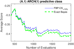
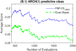
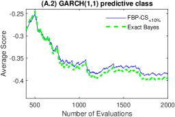
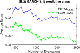
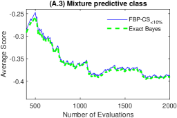
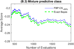
Figure 1: Out-of-sample performance of exact Bayes and CS-based FBP: relative predictive accuracy in the lower tail (Panel A) and the upper tail (Panel B). The three plots in Panel A depict the cumulative average (over an expanding evaluation period) of CS_<10% for the exact Bayes (dashed green line) and FBP-CS_<10% (full blue line) updates, using the ARCH(1), GARCH (1,1) and mixture predictive classes respectively. The three plots in Panel B display the cumulative average of CS_>90% for the exact Bayes (dashed green line) and FBP-CS_>90% (full blue line) updates, using the three different predictive classes.

In Panel B, the superiority of FBP-CS_>90% over exact Bayes, in terms of accurately predicting extremely large returns is in stark evidence. In this case, the relative performance of the two updating methods is less affected by the move from the ARCH(1) to the GARCH(1,1) predictive class. However, once again, use of the more flexible mixture of predictives to underpin the exact Bayes update brings its performance much closer to that of the focused update, with the accuracy of the latter being reasonably robust to the choice of predictive class.

In the following section we provide some insight into why the focused update in the upper tail reaps more benefit out-of-sample than does the lower-tail update, relative to exact Bayes, and the role that misspecification plays here.

4.3.2 Animation of the mean predictives

In Figures 2 and 3 we display animated plots of the one-step-ahead mean predictives produced using expanding windows of $n=500$ to $n=2,499$, and based solely on the (most misspecified) Gaussian ARCH(1) predictive class. The mean predictives produced by both updating methods (FBP and exact Bayes) are superimposed upon the true predictive, produced using simulation from (12)-(14). Figure 2 presents the results for lower tail focus (FBP-CS_<10% versus exact Bayes) and Figure 3 the results for upper tail focus (FBP-CS_>90% versus exact Bayes). The vertical lines in each plot indicate the return that defines the quantile $A$ in (6).

[controls,loop,scale =0.75]3Animate_out_low

Figure 2: Animation over time of mean predictives based on the exact Bayes (dashed green curve) and FBP-CS_<10% (full blue curve) updates. The red curve is the true predictive, produced using simulation from (12)-(14). The predictive class used is Gaussian ARCH(1). The black vertical line denotes the threshold used in the FBP-CS_<10% update, in the production of the mean predictive for time period $n+1.$

[controls,loop,scale =0.75]3Animate_out_up

Figure 3: Animation over time of mean predictives based on the exact Bayes (dashed green curve) and FBP-CS_>90% (full blue curve) updates. The red curve is the true predictive, produced using simulation from (12)-(14). The predictive class used is Gaussian ARCH(1). The black vertical line denotes the threshold used in the FBP-CS_>90% update, in the production of the mean predictive for time period $n+1.$

Two things are clear from Figure 2: one, the lower tails of both the FBP-CS_<10% and exact Bayes predictives are quite similar; two, both tails are - for some time points - quite good at picking up the shape of the true predictive tail, but with the FBP-CS_<10% predictive tail being a better match most of the time. These plots thus provide some explanation of the summary results in Panel A (column 3) of Table 2 and Panel A.1 of Figure 1, in which FBP-CS_<10% dominates exact Bayes, but with the improvement in forecast accuracy being reasonably small, despite the misspecification of the predictive class.

In Figure 3 however, the animated display is very different. The upper tail of the exact Bayes predictive consistently fails to pick up the shape of the true: the misspecified nature of the Gaussian ARCH(1) model has a marked impact on predictive accuracy in this region of the support of $y_{n+1}.$ In contrast, FBP-CS_>90% has the flexibility to focus only what matters - upper tail predictive accuracy - and, as such, produces predictives with upper tails that are much closer in shape to the true, and which are often visually indistinguishable from the true. These plots thus explain the clear numerical dominance of FBP-CS_>90% over exact Bayes in Panel A (column 6) of Table 2 and Panel B.1 of Figure 1.

We finish by noting that focus on upper tail accuracy does - as highlighted by the relevant figures in the middle columns of Panel A in Table 2 - impact quite severely on the ability of FBP- CS_>90% to pick up the lower tail of the true predictive. This outcome highlights the fact that the ex-ante decision as to what form of accuracy to focus on is critical, and most notably so in the very misspecified case.

4.3.3 The differential effect of posterior variation

When adopting the conventional Bayesian paradigm for prediction, a single question needs to be addressed: which model (or set of models) is to be used to produce the predictive distribution? Once that model (or set of models) has been chosen, computational methods are used to integrate out the posterior uncertainty associated with that choice, and a single (marginal) predictive distribution thereby produced. Posterior parameter (and model) uncertainty affects the location, shape, and degree of dispersion of the marginal predictive, and any predictive conclusions drawn from it; however, it is not the convention to explicitly quantify the impact of posterior variation on prediction.

Our new proposal introduces an additional choice into the mix: which measure of predictive accuracy is to drive the production of a predictive distribution? Each different form of in-sample update serves as a different ‘window’ through which a choice of predictive model (or mixture of predictive models) - and all posterior uncertainty associated with that choice - impinges on predictive outcomes. For example, one choice of update may yield a posterior distribution over a given predictive class that is very diffuse; another choice may lead to a very concentrated posterior. Hence, finite sample posterior variation itself has import, since it is not unique, even given a particular choice of predictive class.

We illustrate this point using $M=4,000$ posterior draws from (2) for both FBP-CS_<10% and FBP-CS_>90%, using the Gaussian ARCH(1) predictive class, and for selected values of $n+1$ between $501$ and $2,500$. From the draws from (2) based on the FBP-CS_<10% update, we produce the corresponding $4,000$ values of the ES for period $n+1$ for a portfolio that is ‘long’ in the asset,

$$\text{ES}_{0.1}\left(P_{\bm{\theta}}^{n}\right)=\bm{-}\int_{y<A_{0.1}}yp\left(y|\mathcal{F}_{n},\bm{\theta}\right)dy\text{.}$$ (21)

The integral bound $A_{0.1}$ in (21) denotes the $10\%$ quantile, and ES${}_{0.1}\left(P_{\bm{\theta}}^{n}\right)$ denotes the (negative of the) mean of the random variable $y_{n+1}$ conditional on the future return falling into the lower 10% tail of $p\left(\cdot|\mathcal{F}_{n},\bm{\theta}\right)$; that is, the (negative) expected return in a worst case scenario. For a ‘short’ portfolio, in which extremely large returns are harmful, the relevant function is:

$$\text{ES}_{0.9}\left(P_{\bm{\theta}}^{n}\right)=\int_{y>A_{0.9}}yp\left(y|\mathcal{F}_{n},\bm{\theta}\right)dy,$$ (22)

where $A_{0.9}$ in (22) denotes the $90\%$ quantile, and ES${}_{0.9}\left(P_{\bm{\theta}}^{n}\right)$ denotes the mean of $y_{n+1}$ conditional on the future return falling into the upper 10% tail of $p\left(\cdot|\mathcal{F}_{n},\bm{\theta}\right).$ In this case we produce $4,000$ values of ES${}_{0.9}\left(P_{\bm{\theta}}^{n}\right)$ using the draws from (2) based on the FBP-CS_>90% update. For the Gaussian ARCH(1) predictive class, ES${}_{0.1}\left(P_{\bm{\theta}}^{n}\right)$ and ES${}_{0.9}\left(P_{\bm{\theta}}^{n}\right)$ have closed-form solutions, for any given value of $\bm{\theta}.$

In each case we use kernel density estimation to produce an estimate of the marginal posterior of the scalar ES, based on the $4,000$ draws from (2). As a comparator in each case, we perform the same exercise but using the exact (likelihood-based) Bayes update to define (2). The ‘true’ values of ES_0.1 and ES_0.9, computed using simulation from (12)-(14), are reproduced on the respective plots as red vertical lines. All computations are performed for the selected values of $n+1$, and animated graphics are used to illustrate how all quantities change over time.

[controls,loop,scale =0.75]1Animate_out_long [controls,loop,scale =0.75]1Animate_out_short

Figure 4: Animation over time of the posterior densities for: ES${}_{0.1}\left(\bm{\theta}\right)$ (Panel A), and ES${}_{0.9}\left(\bm{\theta}\right)$ (Panel B). In Panel A, the posterior densities are based on the exact Bayes (dashed green curve) and FBP-CS_<10% (full blue curve) updates. In Panel B, the posterior densities are based on the exact Bayes (dashed green curve) and FBP-CS_>90% (full blue curve) updates. The red vertical line in each panel is the true expected shortfall (ES${}_{0.1}\bm{\ }$in Panel A and ES${}_{0.9}\bm{\ }$in Panel B), produced using simulation from (12)-(14). Note: both on the horizontal axis and in the label for each panel we use the superscript ‘n+1’ to remind the reader that the quantities plotted relate to prediction of ES for time point n+1. In the animation, n+1 in the panel label changes to reflect the actual time point.

From Panel A in Figure 4 we see results that broadly confirm the lack of dominance of the FBP-CS_<10% update over exact Bayes, in terms of accurately reproducing the lower tail of the true predictive. Neither the FBP-based posterior of ES${}_{0.1}\left(P_{\bm{\theta}}^{n}\right)$ (the full blue curve), nor the exact Bayes posterior (the dashed green curve) is located uniformly closer to the true vertical (red) value than the other, across time. That said, the posterior variation in the exact Bayes posterior is always less than that of the FBP posterior, for the selected time points considered.

In contrast, in Panel B in Figure 4 there is a much more marked tendency for the FBP posterior of ES${}_{0.9}\left(P_{\bm{\theta}}^{n}\right)$ to be located closer to the true value of ES_0.9 than is the exact Bayes posterior, in addition to being much more concentrated. Hence, there are several instances over time in which the FBP posterior is extremely concentrated around - or very near to - the true ES: providing a further illustration of the benefits reaped by focusing on upper tail accuracy in the update.

5 Empirical Illustrations

We now illustrate the potential of the focused approach in empirical settings. In Section 5.1 we produce predictive results for two empirical return series, using the same predictive classes adopted in the simulation experiments above. We document the accuracy of the FBP posterior mean predictive in a similar manner to the documentation of the results in Table 2. Furthermore, we illustrate the practical benefits of FBP using two empirically relevant loss measures: one, empirical exceedances for predictive VaRs; two, out-of-sample accuracy for ES, as measured by a consistent class of scoring functions (Ziegel et al.,, 2020). In Section 5.2 we provide a quite different - and ambitious - empirical illustration, by using FBP to predict the 23,000 annual time series from the 2018 ‘M4’ forecasting competition. In all illustrations we estimate the mean predictive in (4) (for the relevant predictive class and updating rule) using (after thinning) 4,000 MCMC posterior draws of $\bm{\theta}$, and base all out-of-sample assessments on this mean predictive. The MCMC scheme remains as described in Appendix B.2, apart from certain minor modifications required for the ‘M4’ example, as detailed in Section 5.2.

5.1 Financial returns

5.1.1 Preliminary diagnostics

The two series used in the first empirical illustration are: i) $4,000$ observations of daily returns on the U.S. dollar currency index (DXY), from 3 Jan 2000 to 3 Nov 2015; and ii) $4,000$ observations of daily returns on the S&P500 index, from 3 Jan 1996 to 3 Feb 2012. Both series are supplied by the Securities Industries Research Centre of Asia Pacific (SIRCA) on behalf of Reuters. All returns are continuously compounded. To match the simulation exercise, the last 2,000 observations in each series are used to perform all out-of-sample assessments, with the one-step-ahead mean predictives produced in the same manner as described in Section 4.3.1 (using expanding estimation samples), apart from the fact that the first estimation sample for both empirical series is of length $n=2,000$ (rather than $n=500$). We also adopt the same three predictive classes, defined by the Gaussian ARCH(1), Gaussian GARCH(1,1) and mixture models.

As tallies with the typical features exhibited by financial returns, the descriptive statistics reported in Table 3 provide evidence of time-varying volatility (significant serial correlation in squared returns) and marginal non-Gaussianity (significant non-normality in the level of returns) in both series. Hence, we can conclude that the simple Gaussian ARCH(1) and GARCH(1,1) predictive classes are likely to be misspecified, and more so than the more flexible mixture class. As such, we would anticipate accuracy gains - by using FBP rather than exact Bayes - to be most in evidence for the ARCH(1) predictive class, with decreasing relative gains expected as the predictive class becomes less misspecified.

	Min	Max	Mean	Median	St.Dev	Range	Skewness	Kurtosis	JB stat	LB stat
DXY	-2.913	1.645	-0.010	-0.007	0.316	4.558	-0.303	4.517	3461	271
S&P500	-21.070	19.510	0.035	0.164	2.590	40.581	-0.260	5.762	5579	2783

Table 3: Summary statistics. ‘JB stat’ is the test statistic for the Jarque-Bera test of normality, with a critical value of 5.99. ‘LB stat’ is the test statistic for the Ljung-Box test of serial correlation in the squared returns; the critical value based on a lag length of 3 is 7.82. ‘Skewness’ is the Pearson measure of sample skewness, and ‘Kurtosis’ a sample measure of excess kurtosis. The labels ‘Min’ and ‘Max’ refer to the smallest and largest value, respectively, while ‘Range’ is the difference between these two. The remaining statistics have the obvious interpretations.

	Panel A: ARCH(1) predictive class
	Out-of-sample score
	Center Focused			Left Focused			Right Focused
	LS	CRPS		FSR10%	FSR20%		FSR80%	FSR90%
Updating method
DXY
Exact Bayes	-0.2528	-0.1701		-0.2810	-0.4113		-0.3953	-0.2729
FBP	-0.2528	-0.1689		-0.2676	-0.3921		-0.3901	-0.2692
S&P500
Exact Bayes	-2.2984	-1.3002		-0.4975	-0.8182		-0.7209	-0.4191
FBP	-2.2984	-1.2922		-0.4661	-0.7859		-0.7100	-0.4090
	Panel B: GARCH(1,1) predictive class
	Out-of-sample score
	Center Focused			Left Focused			Right Focused
	LS	CRPS		FSR10%	FSR20%		FSR80%	FSR90%
Updating method
DXY
Exact Bayes	-0.1798	-0.1664		-0.2484	-0.3712		-0.3832	-0.2660
FBP	-0.1798	-0.1659		-0.2445	-0.3656		-0.3771	-0.2582
S&P500
Exact Bayes	-2.1257	-1.2433		-0.4251	-0.7410		-0.6531	-0.3573
FBP	-2.1257	-1.2422		-0.4213	-0.7350		-0.6510	-0.3569
	Panel C: Mixture predictive class
	Out-of-sample score
	Center Focused			Left Focused			Right Focused
	LS	CRPS		FSR10%	FSR20%		FSR80%	FSR90%
Updating method
DXY
Exact Bayes	-0.1859	-0.1664		-0.2559	-0.3796		-0.3795	-0.2616
FBP	-0.1859	-0.1664		-0.2566	-0.3801		-0.3791	-0.2606
S&P500
Exact Bayes	-2.1261	-1.2437		-0.4239	-0.7397		-0.6543	-0.3586
FBP	-2.1261	-1.2428		-0.4246	-0.7401		-0.6528	-0.3575

Table 4: Predictive accuracy based on FBP and exact Bayes mean predictives. Panels A to C report the average out-of-sample scores for the ARCH(1), GARCH(1,1) and mixture predictive class, respectively. The rows in each panel refer to the update method used. The columns refer to the out-of-sample measure used to compute the average scores. Each FBP figure is based on an update that matches the given out-of-sample accuracy measure. The bold figures are the largest average scores according to a given out-of-sample measure. The two time series are labelled as DXY and S&P500.

	Panel A: Simulated dataset					Panel B: DXY					Panel C: S&P500
	Out-of-sample exceedances					Out-of-sample exceedances					Out-of-sample exceedances
	VaR0.1	VaR0.2	VaR0.8	VaR0.9		VaR0.1	VaR0.2	VaR0.8	VaR0.9		VaR0.1	VaR0.2	VaR0.8	VaR0.9
Updating
method
Exact Bayes	0.117	0.196	0.217	0.062*		0.073*	0.142*	0.157*	0.085		0.081*	0.152*	0.131*	0.060*
FBP-CS<10%	0.102	0.198	0.05*	0.002*		0.084	0.237*	0.027*	0.011*		0.096	0.225*	0.023*	0.008*
FBP-CS<20%	0.103	0.203	0.023*	0.000*		0.077*	0.180	0.059*	0.022*		0.083	0.192	0.039*	0.017*
FBP-CS>80%	0.338*	0.413*	0.197	0.104		0.031*	0.060*	0.204	0.094		0.050*	0.102*	0.164*	0.072*
FBP-CS>90%	0.471*	0.551*	0.148*	0.085		0.015*	0.037*	0.247*	0.100		0.042*	0.074*	0.182*	0.078*

Table 5: Predictive Value at Risk assessment. The figures recorded are the proportion of times that the observed out-of-sample values ‘exceed’ the predictive VaR_α indicated by the column heading. Panels A to C, respectively, record results for the data simulated from (12)-(14), the DXY empirical data, and the S&P500 empirical data. The bold value in each column indicates the empirical coverage that is closest to the nominal tail probability, whilst an asterisk indicates rejection of the null hypothesis of independence and correct coverage at the 1% level of significance, using the Christoffersen test.

In the following sections we assess the relative performance of FBP and exact Bayes for these two series in terms of, respectively: average out-of-sample scores, VaR exceedances, and the average scoring function for ES proposed in Ziegel et al., (2020). For the third exercise, we assess the dominance of FBP over exact Bayes - in terms of predicting ES - by visually comparing the results using the Murphy diagrams proposed in Ehm et al., (2016).

5.1.2 Results: Average out-of-sample scores

In Table 4, we reproduce results for both the likelihood-based update (exact Bayes) and the FBP update that matches the out-of-sample accuracy measure used (as captured by the relevant scoring rule). That is, for each of the two empirical series, and for each predictive class, there is a single row of accuracy results labelled ‘FBP’, with the update underlying the FBP figure in any particular column matching the accuracy measure in the column label.

The results confirm our expectations. In Panel A, the figures based on the ARCH(1) predictive class tell a clear story: using an update that focuses on the measure that is assessed out-of-sample reaps accuracy gains. In all cases, and for both series, the exact (misspecified) Bayesian predictives are out-performed by FBP. In Panel B, FBP based on the GARCH(1,1) class continues to dominate exact Bayes uniformly; however the degree of dominance is less marked than in Panel A. The dominance of FBP over exact Bayes is no longer uniform in Panel C, for the case of the (least misspecified) mixture predictive class. Nevertheless, in all four instances, FBP still out-performs exact Bayes in the upper tail.

Hence, the empirical results mimic the patterns observed in the simulation setting, and continue to send the clear signal: when model misspecification is marked, FBP is beneficial, and particularly in terms of upper tail accuracy in the case of negatively skewed data. In the following sections we assess the practical significance of that benefit by conducting an out-of-sample assessment of the $\alpha\times 100\%$ predictive VaR for period $n+1$ - or predictive quantile (denoted by VaR_α) - and the $\alpha\times 100\%$ ES (denoted by ES_α), both computed from the relevant mean predictive, and for the most misspecified class only: Gaussian ARCH(1). For comparative purposes, we also perform the exercise for the simulated data analyzed in Section 4.3. Note that, for ease of notation we do not make explicit the dependence of both VaR_α and ES_α on a particular predictive distribution, unless this is necessary.

5.1.3 Results: VaR exceedances

To assess predictive accuracy of the VaR, for all updating methods and all return series (both empirical and simulated), we first compute the probability of ‘exceedance’, $\hat{\alpha}$, as the proportion of realized out-of-sample values that are less than the predictive VaR_α for $\alpha=0.1$ and $\alpha=0.2$, as is relevant for a long portfolio. We then compute $1-\hat{\alpha}$, as the proportion of realized values that are greater than the predictive VaR_α for $\alpha=0.8$ and $\alpha=0.9$, as pertains to a short portfolio. Table 5 reports the values of $\hat{\alpha}$ (or $1-\hat{\alpha}$), for the exact Bayes update and four different versions of FBP that focus explicitly on tail accuracy: FBP-CS_<10%, FBP-CS_<20%, FBP-CS_>80% and FBP-CS${}_{>90\%}.$ The bold figure in each column indicates the empirical exceedance that is closest to the nominal tail probability. The asterisk then indicates whether the null hypothesis of $\hat{\alpha}=\alpha$ (or $1-\hat{\alpha}=1-\alpha$) and independence in the exceedances is rejected at the $1\%$ significance level by the Christoffersen, (1998) test. In this particular illustration there is, of course, no exact match between update and out-of-sample measure; however we would anticipate that the FBP methods that focus on accuracy in the lower tail would yield better predictions of VaR_0.1 and VaR_0.2 (and, hence, better associated performance statistics) than would both exact Bayes (with no lower tail focus) and the FBP methods that focus on accuracy in the upper tail; with the corresponding conclusions expected for upper tail focus, and accurate prediction of VaR_0.8 and VaR_0.9. Hence the usefulness of reproducing all five sets of results for each scenario.

Looking first at the bold figures in Table 5, a simple conclusion can be drawn: for all three series, an ‘appropriate’ form of FBP (i.e. with an update that rewards accuracy in the relevant tail) produces empirical exceedances that are closer to the nominal values than do both exact Bayes and the ‘inappropriate’ FBP (i.e. with an update that rewards accuracy in the opposite tail). By this measure, focussing correctly reaps VaR accuracy benefits for all three series. For the DXY series (Panel B) we can hone this conclusion further: the updates that focus on accuracy in a particular marginal tail (remembering that the threshold used in the CS score is based on an estimate of a marginal quantile) also yield the best empirical exceedances for the conditional VaR_α with an equivalent probability. All four bold diagonal exceedances in Panel B are also insignificantly different from the nominal value, and are not associated with rejection of the null of independent violations. Indeed, with the exception of the FBP-CS_>80% exceedance for FBP-CS_>90%, these four diagonal figures are the only ones associated with a failure to reject the joint null of correct coverage and independent violations.

For the data simulated from (12)-(14) (Panel A), with one exception, all FBP methods that focus on the tail that is relevant for VaR_α prediction - so the lower tail for VaR_0.1 and VaR_0.2, and the upper tail for VaR_0.8 and VaR_0.9 - yield statistics that fail to reject the joint null. Moreover, as is somewhat consistent with the particular dominance of FBP over exact Bayes in the upper tail illustrated in Section 4.3.1, there is a slight tendency for FBP to also be more superior to exact Bayes in terms of prediction of the upper tail VaR_α’s. For the S&P500 data, the FBP methods that focus on lower tail accuracy (FBP-CS_<10% and FBP-CS_<20%) are the only ones that do not formally reject the joint null - when used to predict VaR_0.1 and VaR${}_{0.2}.$ However, again, in terms of raw exceedances for VaR_α’s in a particular tail, the FBP methods that reward accuracy in that same tail outperform everything else.

5.1.4 Results: Murphy diagrams for ES predictions

Lastly, we compare the performance of FBP and exact Bayes in terms of the accuracy with which we predict ES. Reiterating that these results are based on the mean predictives (for both FBP and exact Bayes), for the Gaussian ARCH(1) class, this means that in the definition $\text{ES}_{\alpha}(P_{\bm{\theta}}^{n})$ in equations (21)-(22), we replace $P_{\bm{\theta}}^{n}$ with the mean predictive defined in (4), and for both FBP and exact Bayes updating. We then follow Ziegel et al., (2020) and measure the out-of-sample accuracy of both forms of ES predictions using a class of scoring functions that are indexed by some known parameter $\eta\in\mathbb{R}$, and which are consistent for the joint functional of VaR and ES. The specific details of the scoring function, as well as the definition of consistency are delayed until Appendix C.

With reference to a positively-oriented class of consistent scoring functions, Ziegel et al., (2020) say that predictive Method A, e.g. the mean predictive obtained under FBP, dominates predictive method B, e.g. the mean predictive obtained under exact Bayes, if on average predictions of ES obtained under Method A yield a score that is greater than or equal to the score that is obtained under Method B, uniformly over all scoring functions in the class (i.e., all $\eta\in\mathbb{R}$). Sampling variability aside, dominance can then be visualized using the Murphy diagram proposed in Ehm et al., (2016), which plots the average difference between the scores under Methods A and B, over the out-of-sample-evaluation period and across a range of values for $\eta$. For the class of consistent scoring functions defined in Appendix C, and across a grid of values for $\eta$, it is then feasible to evaluate if predictions made using FBP dominate those made under exact Bayes (when both approaches are based on the same predictive class) in terms of their accuracy in predicting ES.

To this end, we produce and discuss Murphy diagrams for both the DXY and S&P500 return series. Panels A.1 and A.2 of Figure 5 present the Murphy diagrams for ES_0.1 and ES_0.2, respectively, for the DXY series. In each panel, predictions based on the ‘appropriate’ form of FBP are compared to exact Bayes. The black solid line displays the average difference (over the out-of-sample period) between the scores calculated under FBP and exact Bayes, across a grid of values for $\eta$. The evaluation period used to calculate the average difference is the same as that used to compute the VaR exceedances in Section 5.1.3. The shaded region corresponds to a 95% bootstrap confidence interval for the average difference, calculated at each $\eta$, based on a block bootstrap (Kunsch,, 1989) with block length of size $b=10$ and $1000$ replications, while the red dashed line is the horizontal line at $y=0$. From these two plots the black line indicates that, for virtually all values of $\eta$, FBP outperforms exact Bayes, since the average score difference is generally positive and the confidence intervals usually do not encompass zero. This result supports the claim that FBP helps improve predictive performance in the lower tail of DXY returns. On the other hand, Panels B.1 and B.2 indicate that no such dominance is observed in terms of the upper-tail ES predictions, although in Panel B.1 the bulk of the confidence intervals do cover positive values, and the FBP forecasts are not dominated by exact Bayes in either panel.

Figure 6 presents the corresponding results for the S&P500 returns. Panels A.1 and B.1 show that there is no dominance of FBP over exact Bayes for ES_0.1 and ES_0.9. On the other hand, Panels A.2 and B.2 show more evidence of FBP having better predictive performance than exact Bayes. In particular, in Panel B.2, for most values of $\eta$ FBP outperforms exact Bayes, with the average score difference being generally positive and most of the confidence intervals not encompassing zero. For completeness we also include the results for the data simulated from (12)-(14). In this case we have illustrated, in Section 4.3.3, the particular accuracy of the FBP-based ES results in the upper 10% tail (relative to exact Bayes). This finding is supported by the stark result in Panel B.1, in which virtually complete dominance of FBP over exact Bayes is on display.

Panel A:	Panel B:
Lower tail expected shortfall	Upper tail expected shortfall

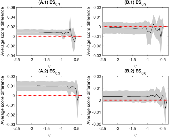
Figure 5: ES predictive performance for the DXY series, measured by the average difference between the FBP and exact Bayes out-of-sample scores. The scoring rule is as defined in (35). Panels (A.1) and (A.2) correspond to ES_0.1 and ES_0.2, respectively; Panels (B.1) and (B.2) correspond to ES_0.9 and ES_0.8, respectively. The solid black line indicates the average difference; the shaded area denotes the 95% bootstrap confidence interval for each $\eta$; and the red dashed line is a horizontal line at zero. Panels (A.1), (A.2), (B.1) and (B.2) are constructed using the FBP-CS${}_{\text{$<$10\%}}$, FBP-CS${}_{\text{$<$20\%}}$, FBP-CS${}_{\text{$>$90\%}}$ and FBP-CS${}_{\text{$>$80\%}}$ methods, respectively, as the relevant FBP method.

Panel A:	Panel B:
Lower tail expected shortfall	Upper tail expected shortfall

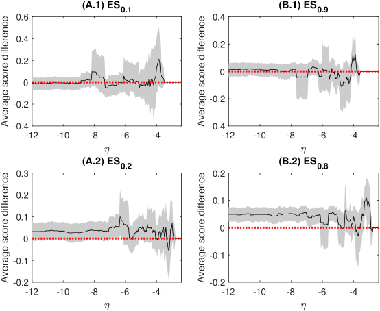
Figure 6: ES predictive performance for the S&P500 series, measured by the average difference between the FBP and exact Bayes out-of-sample scores. The scoring rule is as defined in (35). Panels (A.1) and (A.2) correspond to ES_0.1 and ES_0.2, respectively; Panels (B.1) and (B.2) correspond to ES_0.9 and ES_0.8, respectively. The solid black line indicates the average difference; the shaded area denotes the 95% bootstrap confidence interval for each $\eta$; and the red dashed line is a horizontal line at zero. Panels (A.1), (A.2), (B.1) and (B.2) are constructed using the FBP-CS${}_{\text{$<$10\%}}$, FBP-CS${}_{\text{$<$20\%}}$, FBP-CS${}_{\text{$>$90\%}}$ and FBP-CS${}_{\text{$>$80\%}}$ methods, respectively, as the relevant FBP method.

Panel A:	Panel B:
Lower tail expected shortfall	Upper tail expected shortfall

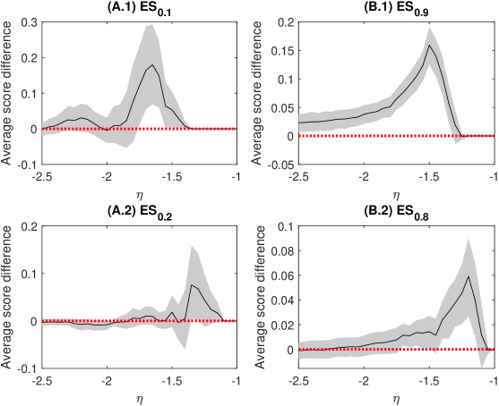
Figure 7: ES predictive performance for the data simulated from (12)-(14), measured by the average difference between the FBP and exact Bayes out-of-sample scores. The scoring rule is as defined in (35). Panels (A.1) and (A.2) correspond to ES_0.1 and ES_0.2, respectively; Panels (B.1) and (B.2) correspond to ES_0.9 and ES_0.8, respectively. The solid black line indicates the average difference; the shaded area denotes the 95% bootstrap confidence interval for each $\eta$; and the red dashed line is a horizontal line at zero. Panels (A.1), (A.2), (B.1) and (B.2) are constructed using the FBP-CS${}_{\text{$<$10\%}}$, FBP-CS${}_{\text{$<$20\%}}$, FBP-CS${}_{\text{$>$90\%}}$ and FBP-CS${}_{\text{$>$80\%}}$ methods, respectively, as the relevant FBP method.

5.2 M4 forecasting competition

The M4 competition was an exploration of forecast performance organized by the University of Nicosia and the New York University Tandon School of Engineering in 2018. A total of 100,000 time series - of differing frequencies and lengths - were made available to the public. Each forecasting expert (or expert team) was then to submit a vector of $h$-step ahead forecasts, $h=1,2,...,H,$ for each of the series. The winner of the competition in a particular category was the expert (team) who achieved the best average out-of-sample predictive accuracy according to the measure of accuracy that defined that category, over all horizons and all series.

One category was concerned with predictive interval accuracy, as measured by the mean scaled interval score (MSIS) proposed in Gneiting and Raftery, (2007). The MSIS formula used in the competition, defined over the $100\left(1-\alpha\right)$% prediction interval, is given by

$$\text{MSIS}=\frac{1}{H}\frac{\sum_{h=1}^{H}\left(u_{t+h}-l_{t+h}+\frac{2}{\alpha}\left(l_{t+h}-y_{t+h}\right)\bm{1}\{y_{t+h}<l_{t+h}\}+\frac{2}{\alpha}\left(y_{t+h}-u_{t+h}\right)\bm{1}\{y_{t+h}>u_{t+h}\}\right)}{\frac{1}{n-m}\sum_{t=m+1}^{n}|y_{t}-y_{t-m}|},$$

where $H$ denotes the longest predictive horizon considered, $l_{t+h}$ and $u_{t+h}$ denote the $100\left(\frac{\alpha}{2}\right)$% and $100\left(1-\frac{\alpha}{2}\right)$% predictive quantile, respectively, $y_{t+h}$ is the realized value at time $t+h$, $h=1,2,...,H$, and $m$ denotes the frequency of the data. The overall predictive accuracy according to this score was measured by the mean MSIS over the 100,000 series.

The fourth best performance in this particular forecasting category was achieved by the ‘M4 team’, who produced prediction intervals using a model with an exponential smoothing structure for the level, trend and seasonal components, and a Gaussian distributional assumption, referred to as the ETS model hereafter (Hyndman et al.,, 2002). All three smoothing components of this model can be either additive or multiplicative in structure, while the trend component can also be specified to be damped; that is, the trend component can be forced to taper off over longer predictive horizons. A variety of ETS specifications were fit to each series using maximum likelihood estimation (MLE), and the best specification then selected via Akaike’s Information Criterion (AIC). The ETS model used to define the predictive interval was then characterized by at most four parameters: $\theta_{1}$, the smoothing parameter in the level; $\theta_{2}$, the smoothing parameter in the trend; $\theta_{3}$, the smoothing parameter in the seasonality; and $\theta$₄ the damping parameter in the trend; with $\bm{z}$ denoting the vector of initial states. The MLEs of the parameters and $\bm{z}$, for the selected model, were then ‘plugged into’ the assumed Gaussian predictive.

We now use the ETS model as the predictive class to which FBP is applied, with the MSIS score used to define the update. To keep the exercise computationally feasible we adopt the same (MLE/AIC-based) strategy as the M4 team for choosing the specification of the ETS model for each series. We also perform the exercise only for the 23,000 annual time series, and for $H=6.$ For each of the $i$ annual series, $i=1,2,...,23,000$, we define: the full sample vector of observations of length $n_{i}$ as $\mathbf{y}_{n_{i}}$; the vector of observations up to time $t$ as $\mathbf{y}_{i,t}$; the observed value at any particular time point $t+h$ as $y_{i,t+h}$; the h-step-ahead $i^{th}$ ETS predictive distribution as $P_{\bm{\theta}_{i}}^{t}$ (with $\bm{\theta}_{i}$ denoting the unknown parameters for the selected model for the $i^{th}$ series); and the $100\left(\frac{\alpha}{2}\right)$% and $100\left(1-\frac{\alpha}{2}\right)$% quantiles of the $i^{th}$ ETS predictive density as $l_{i,t+h}$ and $u_{i,t+h}$ respectively. Using this notation (and acknowledging a slight abuse of the notation used earlier for the one-step-ahead predictives and associated scores), we define the (positively-oriented) MSIS-based sample criterion as $S_{n_{i}}(P_{\bm{\theta}_{i}}^{n_{i}})=\sum\nolimits_{t=0}^{n_{i}-1}S_{MSIS}(P_{\bm{\theta}_{i}}^{t},\bm{y}_{i,t,H}),$ where

$$S_{MSIS}(P_{\bm{\theta}_{i}}^{t},\bm{y}_{i,t,H})=-\frac{1}{{\scriptsize\text{min$\left(H,n_{i}-t\right)$}}}\sum_{h=1}^{\text{min}\left(H,n_{i}-t\right)}\left({}\right. \left.u_{i,t+h}-l_{i,t+h}+\frac{2}{\alpha}\left(l_{i,t+h}-y_{i,t+h}\right)\bm{1}\{y_{i,t+h}<l_{i,t+h}\}\right.$$ (23)

$$+ \left.\frac{2}{\alpha}\left(y_{i,t+h}-u_{i,t+h}\right)\bm{1}\{y_{i,t+h}>u_{i,t+h}\}\right)$$

and $\bm{y}_{i,t,H}=\left(y_{i,t+1},\dots,y_{i,t+\text{min}\left(H,n_{i}-t\right)}\right)^{\prime}$. Because there are 23,000 time series, and associated posteriors of the form of (2), the scale factor for each series $i$, call it $w_{i,n_{i}}$, needs to be selected via a computationally efficient and automated method. We set each $w_{i,n_{i}}$ as $w_{i,n_{i}}=n_{i}d_{\theta_{i}}/2S_{n_{i}}(P_{\hat{\bm{\theta}_{i}}}^{n_{i}}),$ where $\widehat{\bm{\theta}}_{i}$ denotes the MLE of $\bm{\theta}_{i}$, and $d_{\theta_{i}}$ is the dimension of $\bm{\theta}_{i}$. This choice of $w_{i,n_{i}}$ ensures that the scale and convergence of the FBP posterior variance are anchored to those of a well understood benchmark posterior. More details are provided in Appendix B.3. Posterior draws of the ETS predictives for the $i^{th}$ series are defined by the draws of the underlying $\bm{\theta}_{i}$, which are, in turn, produced using the same MCMC scheme described in Appendix B.2 for the GARCH(1,1) model, with appropriate adjustments made for the bounds on the ETS parameters.

Table 6 documents the accuracy with which five alternative methods forecast the 23,000 annual series, with accuracy measured exclusively by the (positively-oriented) MSIS rule. The methods are the top four performers in the full M4 competition (in which all 100,000 series are forecast, and accuracy is measured by MSIS) - denoted by M4-1${}^{\text{st}}$, M4-2${}^{\text{nd}}$, M4-3${}^{\text{rd}}$ and M4-4${}^{\text{th}}$ respectively - and the focused Bayesian method with update based on the MSIS rule, denoted simply by FBP. The four first place-getters are, in brief, the hybrid method of exponential smoothing and recurrent neural networks in Smyl, (2020) (M4-1${}^{\text{st}}$), the feature-based forecast combination method by Montero-Manso et al., (2020) (M4-2${}^{\text{nd}}$), the Card forecasting method in Doornik et al., (2020) (M4-3${}^{\text{rd}}$), with M4-4${}^{\text{th}}$, as noted earlier, being the ETS/MLE-based method of the M4 team. We use the forecasts provided by the competitors (available in the M4 package in R) to assess the predictive accuracy of M4-1${}^{\text{st}}$, M4-2${}^{\text{nd}}$, M4-3${}^{\text{rd}}$ and M4-4${}^{\text{th}}$ for the 23,000 annual series.

	Panel A: Out-of-sample MSIS summaries
	Predictive method
	M4-1${}^{\text{st}}$	M4-2${}^{\text{nd}}$	M4-3${}^{\text{rd}}$	M4-4${}^{\text{th}}$	FBP
Summary
Mean	-23.90	-27.48	-30.20	-34.90	-34.04
Median	-16.18	-16.09	-18.47	-15.49	-14.70
SD	48.17	65.37	65.30	76.84	75.90
Quant 1%	-183.17	-297.98	-214.84	-348.52	-340.00
Quant 10%	-32.23	-28.12	-52.33	-66.71	-65.12
Quant 20%	-24.14	-19.52	-35.07	-34.50	-33.14
Quant 30%	-20.45	-17.72	-27.19	-24.43	-23.28
Quant 40%	-18.02	-16.77	-22.20	-19.02	-17.95
Quant 50%	-16.18	-16.09	-18.47	-15.49	-14.70
Quant 60%	-14.62	-15.54	-15.35	-12.71	-12.21
Quant 70%	-13.29	-15.02	-12.65	-10.45	-10.36
Quant 80%	-12.01	-14.41	-10.43	-8.95	-8.96
Quant 90%	-10.28	-13.41	-8.35	-7.16	-7.03
Quant 99%	-5.29	-7.25	-4.17	-3.30	-3.47
	Panel B: Grouped predictive performance
	Predictive method
	M4-1${}^{\text{st}}$	M4-2${}^{\text{nd}}$	M4-3${}^{\text{rd}}$	M4-4${}^{\text{th}}$	FBP
Time series
group
Group 1	1359	1732	766	304	439
Group 2	814	2136	405	555	690
Group 3	989	558	557	1118	1378
Group 4	522	58	813	1534	1673
Group 5	338	48	1006	1565	1643
Total	4022	4532	3547	5076	5823

Table 6: Predictive accuracy of five competing methods for the 23,000 annual time series from the M4 competition. The labels M4-1${}^{\text{st}}$, M4-2${}^{\text{nd}}$, M4-3${}^{\text{rd}}$ and M4-4${}^{\text{th}}$ denote the first, second, third and fourth best methods (overall) in the MSIS category of M4. The label FBP refers to the focused Bayesian prediction method applied to the ETS predictive class and using the MSIS rule as the update. Panel A records various summaries of the 23,000 (positively-oriented) MSIS values; Panel B reports the number of series for which a particular method performs best in each of the five groups described in the text. The bold font is used to indicate the best performing method according to a given performance measure.

Columns 1 to 4 of Panel A in Table 6 report various summaries of the 23,000 MSIS values - mean, median, standard deviation, and multiple quantiles - for each of the four competition methods. Based on the mean results, the ranking of the four methods for the 23,000 annual series is seen to equal their ranking in the full competition (as indicated by the column labels). Column 5 presents the summary statistics for FBP. First, we observe that both the mean and the median of the MSIS values for FBP are larger than those for M4-4${}^{\text{th}}$ (ETS/MLE), which indicates that focusing does enhance predictive performance over and above simple use of the maximizer of the likelihood function of the (inevitably misspecified) ETS model. Second, we observe that in terms of median MSIS, FBP produces the best results out of all five methods considered. By looking at the quantiles of the distribution of the 23,000 scores for all methods we can glean why this is so. In particular, the values of MSIS at the 1^st quantile for M4-4${}^{\text{th}}$ and FBP are -348.52 and -340.00 respectively, whilst for M4-1${}^{\text{st}}$, M4-2${}^{\text{nd}}$ and M4-3${}^{\text{rd}}$ the corresponding values are -183.17, -297.98 and -214.84, respectively. In other words both ETS-based methods forecast 1% of the series quite poorly, which impacts on their mean MSIS. In contrast, the ETS-based methods - and particularly FBP - forecast quite accurately those series that produce MSIS values that are in the middle of the distribution, or in the upper tail.

To provide further insight here, we divide the 23,000 series into five different groups of 4,600 series. Group 1 has the 4,600 series with the smallest average MSIS, computed across the five methods (i.e. the series with the worst average results according to this measure), while Group 5 comprises the 4,600 series with the largest average MSIS values. The remaining groups span the middle. For each of these groups we count how many series are best predicted by each of the five methods. The results are presented in Panel B of Table 6. First, we observe that for all groups FBP has a larger number of favourable results than does the likelihood-based ETS method (M4-4${}^{\text{th}}$). Second, for the last three groups FBP outperforms all four other methods. Last, observe that the method that is best at predicting the highest number of series overall is FBP, with a total of 5,823 series (out of 23,000) for which it is the best performer. Focusing on predictive interval accuracy in the update has clearly yielded benefits out-of-sample.

6 Discussion

We have proposed a new paradigm for Bayesian prediction that can deliver accurate predictions in whatever metric is most meaningful for the problem at hand. By replacing the conventional likelihood function in the Bayesian update with an appropriate function of a proper scoring rule, the resultant posterior - by construction - gives high probability mass to predictive distributions that yield high scores. Under regularity, the posterior asymptotically concentrates onto the predictive that maximizes the expected scoring rule and, in this sense, yields the most accurate predictions in the given class. Movement away from the conventional Bayesian approach does involve the choice of a scale factor, which determines the relative weight of the prior and data-based components of the posterior. However, this factor can be chosen via common sense criteria in finite samples.

The choice of predictive class used is not pre-determined, and can be any plausible class of predictives, or combination of predictives, that captures the features of the data that matter for prediction. In particular, the class can be deliberately selected to be computationally simple; the aim of the approach not being to perfectly capture all aspects of the true DGP, but to achieve a particular type of predictive accuracy via a suitable Bayesian update. Whilst the emphasis in the paper has been on classes of parametric predictives, or finite combinations of predictives, the paradigm, in principle, applies to nonparametric predictive settings also. Similarly, the focus on time series data, and ‘forecasting’ future values of random variables indexed by time, has also been a choice on our part, and not something that is intrinsic to the methodology.

The scope and value of our new approach to prediction are demonstrated using illustrations with simulated and empirical data. The benefits reaped by ‘focusing’ on the type of predictive accuracy that matters are stark, with virtually all numerical results showing gains over and above conventional (misspecified) likelihood-based prediction. Whilst a reduction in the degree of misspecification of the predictive class does lead to more homogeneous predictions across methods, for a large enough sample the superiority of FBP is still almost always in evidence, even when the predictive class is a reasonable representation of the true DGP.

Some obvious avenues of future research remain open. First, the ability to generate accurate predictions via a simplistic representation of the truth means that models with, for example, intractable likelihood functions, can now be treated using exact simulation methods like MCMC, rather than via approximate methods like approximate Bayesian computation (Sisson et al.,, 2018) or Bayesian synthetic likelihood (Price et al.,, 2018). Comparison between the results yielded by FBP and those yielded by predictives based on such approximate methods of inference (e.g. Frazier et al.,, 2019) would be of interest. Second, in cases where the set of unknowns is very large, and an MCMC simulation method is likely to be inefficient, variational methods could be explored. In particular - and in the spirit of the generalized variational inference proposed by Knoblauch et al., (2019) - the choice of variational family, and/or the distance measure to be minimized, could be driven by the specific prediction focus of any problem. Finally, all results in this paper have been based on proper scoring rules only. This is by no means essential, but has simply been a decision made to render the scope of the paper manageable. In practice, any loss function in which predictive accuracy plays a role (e.g. financial loss functions associated with optimal portfolios of predicted returns; asymmetric loss functions associated with predicted energy demand) can drive the Bayesian update, and thereby give high weight to predictive distributions that yield small loss.

Appendix A Assumptions and Proofs of Main Results

Consider a stochastic process $\{y_{t}:\Omega\rightarrow\mathbb{R},t\in\mathbb{N}\}$ defined on the complete probability space $(\Omega,\mathcal{F},P)$. Let $\mathcal{F}_{t}:=\sigma(y_{1},\dots,y_{t})$ denote the natural sigma-field. The model predictive class is given by $\mathcal{P}^{t}:=\left\{P_{\bm{\theta}}^{t}:\bm{\theta}\in\Theta\right\}$, where the parameter space is a (possibly non-compact) subset of the Euclidean space $\Theta\subseteq\mathbb{R}^{d_{\theta}}$, with $d_{\theta}$ the dimension of $\bm{\theta}$, and where for any $A\subset\mathcal{F}$, $P_{\bm{\theta}}^{t}(A):=P(A|\mathcal{F}_{t},\bm{\theta})$.

Define the $\delta$-neighborhood of $\Theta$, around the point $\bm{\theta}_{\ast}$, as $\mathcal{N}_{\delta}(\bm{\theta}_{\ast}):=\{\bm{\ \theta}:\|\bm{\theta}-\bm{\theta}_{\ast}\|\leq\delta\},$ where $\|\cdot\|$ denotes the Euclidean norm. We say two sequences $x_{n}$ and $z_{n}$ satisfy $x_{n}\lesssim z_{n}$ if there is a constant $C>0$ and an $n^{\prime}$ such that for all $n>n^{\prime}$, $x_{n}\leq Cz_{n}$. Throughout the remainder, we let $C$ denote a generic constant that can change from line to line.

With a slight change in notation, recall the empirical scoring rule calculated from $\mathbf{y}_{n}$:

$$S_{n}(\bm{\theta}):=\sum_{t=0}^{n-1}S(P_{\bm{\theta}}^{t},y_{t+1}),$$

and recall the limit optimizer,

$$\bm{\theta}_{\ast}:=\arg\max_{P_{\bm{\theta}}^{t}\in\mathcal{P}}\left[\operatorname*{plim}_{n\rightarrow\infty}\sum_{t=0}^{n-1}S(P_{\bm{\theta}}^{t},y_{t+1})/v_{n}^{2}\right],$$

for $v_{n}$ a positive sequence diverging to $\infty$ as $n\rightarrow\infty$. The value $\bm{\theta}_{\ast}$ corresponds to the predictive $P_{\bm{\theta}}^{t}\in\mathcal{P}^{t}$ such that, in the limit, we minimize the expected (i.e., asymptotic) loss, in terms of $S(\cdot,y)$, between the assumed predictive class, $\mathcal{P}$, and the true DGP that underlies the observed values of $y_{t+1}.$

We consider the following regularity conditions on the function $S_{n}$ and the prior $\pi(\cdot)$.

Assumption 1.

The prior density $\pi(\bm{\theta})$ is continuous on $\|\bm{\theta}-\bm{\theta}_{*}\|\leq\delta$, for some $\delta>0$, and positive for all $\bm{\theta}\in\Theta$. In addition, for any $t>0$, and any $\kappa$, $0<\kappa<\infty$, there exists some $C>0$, and $p>\kappa$ such that

$$\Pi\left(\|\bm{\theta}-\bm{\theta}_{*}\|>t\right)\leq Ct^{-p}.$$

Assumption 2.

There exists a sequence $v_{n}$ diverging to $\infty$ such that, for any $\delta>0$ there exists some $\epsilon>0$,

$$\lim\inf_{n\rightarrow\infty}\text{\emph{Pr}}\left\{\sup_{\bm{\ \theta}\in\mathcal{N}^{c}_{\delta}(\bm{\theta}_{*})}\frac{1}{v_{n}^{2}}\left[S_{n}(\bm{\theta})-S_{n}(\bm{\theta}_{*})\right]\leq-\epsilon\right\}=1.$$

Assumption 3.

For some $\delta>0$, the following are satisfied uniformly for $\bm{\theta}\in\mathcal{N}_{\delta}(\bm{\theta}_{*})$: There exists a sequence $v_{n}$ diverging to $\infty$, a vector function $\bm{\Delta}_{n}(\bm{\theta})$, matrices $H_{n}$ and $V_{n}$, such that

1. $S_{n}(\bm{\theta})-S_{n}(\bm{\theta}_{*})=v_{n}\left(\bm{\theta}-\bm{\theta}_{*}\right)^{\prime}\bm{\Delta}_{n}\left(\bm{\theta}_{*}\right)/v_{n}-\frac{1}{2}v_{n}\left(\bm{\theta}-\bm{\theta}_{*}\right)^{\prime}H_{n}v_{n}\left(\bm{\theta}-\bm{\theta}_{*}\right)+R_{n}(\bm{\theta})$

2. $V_{n}^{-1/2}\bm{\Delta}_{n}\left(\bm{\theta}_{*}\right)/v_{n}\Rightarrow N(\bm{0},I)$ under $P$.

3. For $n$ large enough, $H_{n}$ is positive-definite and, for some matrix $H$, $H_{n}\rightarrow_{p}H$.

4. For any $\epsilon>0$, there exists $M\rightarrow\infty$ and $\delta=o(1)$ such that

   $$\lim\sup_{n\rightarrow\infty} \text{\emph{Pr}}\left[\sup_{\frac{M}{v_{n}}\leq\|\bm{\theta}-\bm{\theta}_{*}\|\leq\delta}\frac{|R_{n}(\bm{\theta})|}{v_{n}^{2}\|\bm{\theta}-\bm{\theta}_{*}\|^{2}}>\epsilon\right]<\epsilon\text{ and }\lim\sup_{n\rightarrow\infty} \text{\emph{Pr}}\left[\sup_{\|\bm{\theta}-\bm{\theta}_{*}\|\leq\frac{M}{v_{n}}}\frac{|R_{n}(\bm{\theta})|}{v_{n}^{2}\|\bm{\ \theta}-\bm{\theta}_{*}\|^{2}}>\epsilon\right]=0$$

Remark 4.

The use of $v_{n}$ in the assumptions allows us to capture cases where the scoring rules may converge at rates other than the canonical $\sqrt{n}$. Such instances include situations where the data are trended or otherwise non-stationary.

Remark 5.

Assumption 1 places regularity conditions on the prior used within the analysis and is standard in the literature on Bayesian inference. Assumptions 2 and 3 are sufficient conditions that can be used to deduce $v_{n}$-consistency and asymptotic normality of the M-estimator based on minimizing $S_{n}(\bm{\theta})$, with these assumptions being similar to those used in Chernozhukov and Hong, (2003). These assumptions are reasonable in any setting where the resulting M-estimator is expected to display regular asymptotic behavior. In the case of log-score, these assumptions are akin to the usual sufficient conditions used to demonstrate consistency and asymptotic normality of the quasi-maximum likelihood estimator. Indeed, in the context of the log-score, Assumptions 2 and 3 can be directly verified, for example, for the ARCH(1) and GARCH(1,1) models used in Sections 4 and 5.1 using the results of Lee and Hansen, (1994). However, we remark that the validation of Assumptions 2 and 3 in the context of other models, and other scoring rules, such as the censored score, CRPS or MSIS, entails substantive technical challenges that are best analyzed in future work.

A.1 Posterior concentration

Consider the FBP posterior pdf

$$\pi_{w}\left(\bm{\theta}|\mathbf{y}_{n}\right)=\frac{\exp\left[w_{n}S_{n}({\bm{\theta}})\right]\pi(\bm{\theta})}{\int_{\Theta}\exp\left[w_{n}S_{n}({\bm{\theta}})\right]\pi(\bm{\theta})\text{d}\bm{\theta}}.$$ (24)

Under Assumptions 1-3, we prove a generalization of the result in Lemma 2, which demonstrates that the scaled posterior ${\tilde{\pi}}_{w}\left({\bm{\eta}}|\mathbf{y}_{n}\right):=\pi_{w}(\bm{\theta}|\mathbf{y}_{n})/v_{n}$, where $\pi_{w}(\bm{\theta}|\mathbf{y}_{n})$ is defined in (24), converges to a Gaussian version in the total variation of moments norm. The result of Lemma 1 then follows by taking $v_{n}=\sqrt{n}$ and considering the standard definition of $S_{n}(\bm{\theta})$.

Proposition 1.

For

$$\bm{\eta}:=v_{n}\left(\bm{\theta}-\bm{\theta}_{*}\right)-H_{n}^{-1}\bm{\Delta}_{n}\left(\bm{\theta}_{*}\right)/v_{n},$$

and

$$\phi\left(\bm{\eta}|H_{n}\right):=Q_{n}\exp\left[-\frac{C}{2}\bm{\eta}^{\prime}H_{n}\bm{\eta}\right]$$

with $Q_{n}:=\sqrt{C\text{det}\left[H_{n}\right](2\pi)^{-d_{\theta}}}$, if Assumptions 1-3 are satisfied and $\lim_{n}w_{n}=C$, $0<C<\infty$, then

$$\int\left[1+\|\bm{\eta}\|^{\kappa}\right]\left|\left.\tilde{\pi}_{w}(\bm{\eta}|\mathbf{y}_{n})-\phi\left(\bm{\eta}|H_{n}\right)\right.\right|\text{d}\bm{\eta}=o_{p}(1).$$

Proof.

Define

$$\bm{L}_{n}:=\bm{\theta}_{*}+H_{n}^{-1}\bm{\Delta}_{n}(\bm{\theta}^{*})/v_{n}^{2}$$

and note that by a change of variables $\bm{\theta}\mapsto\bm{\eta}$, we obtain the posterior

$$\tilde{\pi}[\bm{\eta}|\mathbf{y}_{n}]:=\frac{\pi\left(\bm{\eta}/v_{n}+\bm{L}_{n}\right)\exp\left[w_{n}S_{n}(\bm{\eta}/v_{n}+\bm{L}_{n})\right]}{\int\pi\left(\bm{u}/v_{n}+\bm{L}_{n}\right)\exp\left[w_{n}S_{n}(\bm{u}/v_{n}+\bm{L}_{n})\right]\text{d}\bm{u}}.$$

Define

$$\gamma(\bm{\eta}):=S_{n}\left(\bm{\eta}/v_{n}+\bm{L}_{n}\right)-S_{n}(\bm{\theta}_{*})-\frac{1}{2v_{n}^{2}}\Delta_{n}(\bm{\theta}_{*})^{\prime}H^{-1}_{n}\Delta_{n}(\bm{\theta}_{*})$$

and note that

$$\tilde{\pi}[\bm{\eta}|\mathbf{y}_{n}]:=\frac{\pi\left(\bm{\eta}/v_{n}+\bm{L}_{n}\right)\exp\left(w_{n}\gamma(\bm{\eta})\right)}{C_{n}},$$

for

$$C_{n}=\int\pi\left(\bm{u}/v_{n}+\bm{L}_{n}\right)\exp(w_{n}\cdot\gamma(\bm{u}))\text{d}\bm{u}.$$

Note that we can write

$$\int\|\bm{\eta}\|^{\kappa}\left|\tilde{\pi}\right(\bm{\eta}|\mathbf{\ y}_{n}\left)-\phi\left(\bm{\eta}|H_{n}\right)\right|\text{d}\bm{\eta} =\frac{1}{C_{n}}\int\|\bm{\eta}\|^{\kappa}{|}e^{w_{n}\gamma(\bm{\eta})}\pi\left(\bm{\eta}/v_{n}+\bm{L}_{n}\right)-\phi\left(\bm{\eta}|H_{n}\right)C_{n}{|}\text{d}\bm{\eta}$$

$$={J_{n}}/{C_{n}},$$

where

$$J_{n}: =\int\|\bm{\eta}\|^{\kappa}\left|e^{w_{n}\gamma(\bm{\eta})}\pi\left(\bm{\eta}/v_{n}+\bm{L}_{n}\right)-\phi\left(\bm{\eta}|H_{n}\right)C_{n}\right|\text{d}\bm{\eta}.$$ (25)

Now, bound $J_{n}$ as follows

$$J_{n} \leq\int\|\bm{\eta}\|^{\kappa}\left\{\left|e^{w_{n}\gamma(\bm{\eta})}\pi\left(\bm{\eta}/v_{n}+\bm{L}_{n}\right)-\pi\left(\bm{\theta}_{*}\right)\phi\left(\bm{\eta}|H_{n}\right){\color[rgb]{0,0,0}\text{$Q_{n}^{-1}$}}\right|+\left|\left[\pi\left(\bm{\theta}_{*}\right){\color[rgb]{0,0,0}\text{$Q_{n}^{-1}$}}-{C}_{n}\right]\phi\left(\bm{\eta}|H_{n}\right)\right|\right\}\text{d}\bm{\eta},$$

$$\leq J_{1n}+J_{2n},$$

where

$$J_{1n} :=\int\|\bm{\eta}\|^{\kappa}\left|e^{w_{n}\gamma(\bm{\eta})}\pi\left(\bm{\eta}/v_{n}+\bm{L}_{n}\right)-\pi\left(\bm{\theta}_{*}\right)\phi\left(\bm{\eta}|H_{n}\right){\color[rgb]{0,0,0}\text{$Q_{n}^{-1}$}}\right|\text{d}\bm{\eta}$$ (26)

$$J_{2n} :=\left|\pi(\bm{\theta}_{*}){\color[rgb]{0,0,0}\text{$Q_{n}^{-1}$}}-C_{n}\right|\int\|\bm{\eta}\|^{\kappa}\phi\left(\bm{\eta}|H_{n}\right)\text{d}\bm{\eta}$$ (27)

The result follows if we can prove that $J_{1n}=o_{p}(1)$ since, taking $\kappa=0$, $J_{1n}=o_{p}(1)$ implies that

$$\left|C_{n}-\pi(\bm{\theta}_{*}){\color[rgb]{0,0,0}\text{$Q_{n}^{-1}$}}\right| =\left|\int e^{w_{n}\gamma(\bm{\eta})}\pi\left(\bm{\eta}/v_{n}+\bm{L}_{n}\right)\text{d}\bm{\eta}-\pi(\bm{\theta}_{*}){\color[rgb]{0,0,0}\text{$Q_{n}^{-1}$}}\int\phi\left(\bm{\eta}|H_{n}\right)\text{d}\bm{\eta}\right|$$

$$=o_{p}(1),$$

which implies that $J_{2n}=o_{p}(1)$ and therefore $J_{n}=o_{p}(1)$.

Using Assumption 3.1, the fact that $(\bm{\theta}-\bm{\theta}_{*})=\left(\bm{\eta}-\bm{\eta}_{n}^{*}\right)/v_{n}$ with $\bm{\eta}_{n}^{*}:=-H_{n}^{-1}\bm{\Delta}_{n}/v_{n}$, and the definitions of $\bm{L}_{n}$ and $\gamma(\bm{\eta})$, we re-express $\gamma(\bm{\eta})$ as

$$\gamma(\bm{\eta}) =S_{n}\left(\bm{\theta}\right)-S_{n}(\bm{\theta}_{*})-\frac{1}{2v_{n}^{2}}\bm{\Delta}_{n}(\bm{\ \theta}_{*})^{\prime}{\color[rgb]{0,0,0}\text{$H_{n}^{-1}$}}\bm{\Delta}_{n}(\bm{\theta}_{*})$$

$$=\frac{\left(\bm{\eta}-\bm{\eta}_{n}^{*}\right)}{v_{n}}^{\prime}\bm{\Delta}_{n}(\bm{\theta}_{*})-\frac{v^{2}_{n}}{2}\frac{\left(\bm{\eta}-\bm{\eta}_{n}^{*}\right)}{v_{n}}^{\prime}H_{n}\frac{\left(\bm{\eta}-\bm{\eta}_{n}^{*}\right)}{v_{n}}-\frac{1}{2v_{n}^{2}}\bm{\Delta}_{n}(\bm{\theta}_{*})^{\prime}{\color[rgb]{0,0,0}\text{$H_{n}^{-1}$}}\bm{\ \Delta}_{n}(\bm{\theta}_{*})+R_{n}\left(\bm{\eta}/v_{n}+\bm{L}_{n}\right)$$

$$=-\frac{1}{2}{\bm{\eta}^{\prime}}H_{n}{\bm{\eta}}+R_{n}\left(\bm{\eta}/v_{n}+\bm{L}_{n}\right).$$

To demonstrate that $J_{1n}=o_{p}(1)$, we split the integral for $J_{1n}$ into three regions: for $0<M<\infty$, and some $\delta>0$,

1. $\|\bm{\eta}\|\leq M$

2. $M<\|\bm{\eta}\|\leq\delta v_{n}$

3. $\|\bm{\eta}\|\geq\delta v_{n}$.

Area 1: Over $\|\bm{\eta}\|\leq M$,

$$\sup_{\|\bm{\eta}\|\leq M} \left|\pi\left(\bm{\eta}/v_{n}+\bm{L}_{n}\right)-\pi(\bm{\theta}_{*})\right|=o_{p}(1),$$

$$\sup_{\|\bm{\eta}\|\leq M} \left|R_{n}\left(\bm{\eta}/v_{n}+\bm{L}_{n}\right)\right|=o_{p}(1).$$

The first result follows from continuity of $\pi(\cdot)$ in Assumption 1, the convergence of $\bm{\Delta}_{n}(\bm{\theta}_{*})$ in Assumption 3.2, and the definition of $\bm{L}_{n}$. The second result follows from the second part of Assumption 3.4. The dominated convergence theorem then allows us to deduce that $J_{1n}=o_{p}(1)$ over $\|\bm{\eta}\|\leq M$.

Area 2: Over $M\leq\|\bm{\eta}\|\leq\delta v_{n}$, the second term in the integral can be made arbitrarily small by taking $M$ large enough and $\delta=o(1)$. It therefore suffices to show that, for $M$ large enough and $\delta$ small enough,

$$\tilde{J}_{1n}:=\int_{M\leq\|\bm{\eta}\|\leq\delta v_{n}}\|\bm{\eta}\|^{\kappa}\exp\left[w_{n}\gamma(\bm{\eta})\right]\pi\left(\bm{\eta}/v_{n}+\bm{L}_{n}\right)\text{d}\bm{\eta}=o_{p}(1).$$

From the definition of $\gamma(\bm{\eta})$, it follows that

$$\exp\left[w_{n}\gamma(\bm{\eta})\right]\leq\exp\left[-\frac{w_{n}}{2}\bm{\eta}^{\prime}H_{n}\bm{\eta}+w_{n}\left|R_{n}\left(\bm{\eta}/v_{n}+\bm{L}_{n}\right)\right|\right].$$

By the first part of Assumption 3.4, on the set $\{\bm{\eta}:M\leq\|\bm{\eta}\|\leq\delta v_{n}\}$,

$$\left|R_{n}\left(\bm{\eta}/v_{n}+\bm{L}_{n}\right)\right| =o_{p}\left(v_{n}^{2}\|v_{n}^{-1}\left[\bm{\eta}-\bm{\eta}_{n}^{*}\right]\|^{2}\right)=o_{p}\left(\|\bm{\eta}+\frac{1}{v_{n}}H_{n}^{-1}\bm{\Delta}_{n}\|^{2}\right).$$

Since $\|\bm{\eta}_{n}^{*}\|^{2}=O_{p}(1)$, we conclude that, for some $C>0$, on the set $A_{M,\delta}=\{\bm{\eta}:M\leq\|\bm{\eta}\|\leq\delta v_{n}\}$,

$$\exp\left[w_{n}\gamma(\bm{\eta})\right]\leq C\exp\left[-\frac{w_{n}}{2}\bm{\eta}^{\prime}H_{n}\bm{\eta}+o_{p}\left(w_{n}\|\bm{\ \eta}\|^{2}\right)\right].$$

We then have that, for some $M\rightarrow\infty$, $\tilde{J}_{1n}\leq K_{1n}+K_{2n}+K_{3n}$, where

$$K_{1n}:= \int_{A_{M,\delta}}\|\bm{\eta}\|^{\kappa}\exp\left(-\frac{w_{n}}{2}\bm{\eta}^{\prime}H_{n}\bm{\eta}\right)\sup_{\|\bm{\ \eta}\|\leq M}\left|\exp\left[o_{p}\left(w_{n}\|\bm{\eta}\|^{2}\right)\right]\pi\left(\bm{\eta}/v_{n}+\bm{L}_{n}\right)-\pi\left(\bm{\theta}_{*}\right)\right|\text{d}\bm{\eta}$$

$$K_{2n}:= \int_{A_{M,\delta}}\|\bm{\eta}\|^{\kappa}\exp\left[-\frac{w_{n}}{2}\bm{\eta}^{\prime}H_{n}\bm{\eta}+o_{p}\left(w_{n}\|\bm{\ \eta}\|^{2}\right)\right]\pi\left(\bm{\eta}/v_{n}+\bm{L}_{n}\right)\text{d}\bm{\eta}$$

$$K_{3n}:= \pi\left(\bm{\theta}_{*}\right)\int_{A_{M,\delta}}\|\bm{\eta}\|^{\kappa}\exp\left[-\frac{w_{n}}{2}\bm{\eta}^{\prime}H_{n}\bm{\eta}+o_{p}\left(w_{n}\|\bm{\eta}\|^{2}\right)\right]\text{d}\bm{\eta}$$

For any fixed $M$, $K_{1n}=o_{p}(1)$, hence, for some sequence $M\rightarrow\infty$, by the dominated convergence theorem, it follows that $K_{1n}=o_{p}(1)$. For the second and third terms, we note the following:

(i) For any $0<\kappa<\infty$, on the set $\{\bm{\eta}:\|\bm{\eta}\|\geq M\}$, there exists some $M^{\prime}$ large enough such that for all $M>M^{\prime}$:

$$\|\bm{\eta}\|^{\kappa}\exp\left(-\bm{\eta}^{\intercal}H_{n}\bm{\eta}\right)=O(1/M).$$

(ii) From the definition of $\bm{L}_{n}$, $\bm{L}_{n}\rightarrow_{p}\bm{\theta}_{*}$ and by continuity of $\pi(\cdot)$, on the set $\{\bm{\eta}:M\leq\|\bm{\eta}\|\leq\delta v_{n}\}$, for $\delta=o(1)$, we conclude that

$$\pi(\bm{L}_{n}+\bm{\eta}/v_{n})=\pi(\bm{\theta}_{*})+o_{p}(1).$$

Applying (i) yields $K_{3n}=o_{p}(1)$. Applying (i) and (ii) together yields $K_{2n}=o_{p}(1)$.

Area 3: Over $\|\bm{\eta}\|\geq\delta v_{n}$. For $\delta v_{n}$ large

$$Q_{n}^{-1}\int_{\|\bm{\eta}\|\geq\delta v_{n}}\|\bm{\eta}\|^{\kappa}\phi(\bm{\eta}|H_{n})\pi(\bm{\theta}_{*})\text{d}\bm{\eta}=o(1).$$

Now, focus on

$$\tilde{J}_{1n}:=\int_{\|\bm{\eta}\|\geq\delta v_{n}}\|\bm{\eta}\|^{\kappa}e^{w_{n}\gamma(\bm{\eta})}\pi\left(\bm{\ \eta}/v_{n}+L_{n}\right)\text{d}\bm{\eta}.$$

The change of variables $\bm{\theta}=\bm{\eta}/v_{n}+\bm{L}_{n}$, then yields

$$\tilde{J}_{1n}=v_{n}^{d_{\theta}+\kappa}\int_{\|\bm{\theta}-\bm{L}_{n}\|\geq\delta}\|\bm{\theta}-\bm{L}_{n}\|^{\kappa}e^{w_{n}\left[S_{n}(\bm{\theta})-S_{n}(\bm{\theta}_{*})-\frac{1}{2v_{n}^{2}}\bm{\ \Delta}_{n}(\bm{\theta}_{*})^{\prime}H_{n}^{-1}\bm{\Delta}_{n}(\bm{\theta}_{*})\right]}\pi\left(\bm{\theta}\right)\text{d}\bm{\theta}.$$

Use the fact that $\bm{L}_{n}=\bm{\theta}_{*}+o_{p}(1)$, and bound $\tilde{J}_{1n}$ by

$$Ce^{-\frac{w_{n}}{2v_{n}^{2}}\bm{\Delta}_{n}(\bm{\theta}_{*})^{\prime}H_{n}^{-1}\bm{\Delta}_{n}(\bm{\theta}_{*})}v_{n}^{d_{\theta}+\kappa}\int_{\|\bm{\theta}-\bm{\theta}_{*}\|\geq\delta}\|\bm{\theta}-\bm{\theta}_{*}\|^{\kappa}e^{w_{n}\left[S_{n}(\bm{\theta})-S_{n}(\bm{\theta}_{*})\right]}\pi\left(\bm{\theta}\right)\text{d}\bm{\theta},$$

From Assumption 3.2, $\frac{1}{2v_{n}^{2}}\bm{\Delta}_{n}(\bm{\theta}_{*})^{\prime}H_{n}^{-1}\bm{\Delta}_{n}(\bm{\theta}_{*})=O_{p}(1)$ so that $e^{-\frac{w_{n}}{2v_{n}^{2}}\bm{\Delta}_{n}(\bm{\theta}_{*})^{\prime}H_{n}^{-1}(\bm{\theta}_{*})\bm{\Delta}_{n}(\bm{\theta}_{*})}=O_{p}(1)$. By Assumption 2, for any $\delta>0$, there exists some $\epsilon>0$ such that

$$\lim_{n\rightarrow\infty}\text{Pr}\left\{\sup_{\|\bm{\theta}-\bm{\theta}_{*}\|\geq\delta}\left[S_{n}(\bm{\theta})-S_{n}(\bm{\theta}_{*})\right]\leq-v_{n}^{2}\epsilon\right\}=1.$$

Applying the above conclusion to $\tilde{J}_{1n}$ then yields, for $w_{n}$ a positive convergence sequence, for $n$ large enough,

$$\tilde{J}_{1n}\lesssim e^{-\epsilon w_{n}v_{n}^{2}}v_{n}^{d_{\theta}+\kappa}\int_{\|\bm{\theta}-\bm{\theta}_{*}\|\geq\delta}\|\bm{\theta}-\bm{\theta}_{*}\|^{\kappa}\pi\left(\bm{\theta}\right)\text{d}\bm{\theta}.$$

Apply the above bound, Assumption 1, and the dominated convergence theorem to deduce

$$\tilde{J}_{1n}\lesssim e^{-\epsilon w_{n}v_{n}^{2}}v_{n}^{d_{\theta}+\kappa}\int_{\|\bm{\theta}-\bm{\theta}_{*}\|\geq\delta}\|\bm{\theta}-\bm{\theta}_{*}\|^{\kappa}\pi\left(\bm{\theta}\right)\text{d}\bm{\theta} \lesssim e^{-\epsilon w_{n}v_{n}^{2}}v_{n}^{d_{\theta}+\kappa}\int_{\|\bm{\theta}-\bm{\ \theta}_{*}\|\geq\delta}\|\bm{\theta}-\bm{\theta}_{*}\|^{\kappa}\pi\left(\bm{\theta}\right)\text{d}\bm{\theta}+o_{p}(1)$$

$$\leq e^{-\epsilon w_{n}v_{n}^{2}}v_{n}^{d_{\theta}+\kappa}\int\|\bm{\ \theta}-\bm{\theta}_{*}\|^{\kappa}\pi\left(\bm{\theta}\right)\text{d}\bm{\theta}+o_{p}(1)$$

$$\lesssim e^{-\epsilon w_{n}v_{n}^{2}}v_{n}^{d_{\theta}+\kappa}+o_{p}(1).$$

∎

A.2 Bayesian and frequentist agreement

We now prove the result of Lemma 2 and, subsequently, Theorem 1.

Proof of Lemma 2.

We first prove that the sequence $\|\widehat{\bm{\theta}}-\bm{\theta}_{*}\|=O_{p}(v_{n}^{-1})$. By assumption,

$$o_{p}(v_{n}^{-1})\leq S_{n}(\hat{\bm{\theta}})-S_{n}(\bm{\theta}_{*}).$$

Applying 3.1 to the above we obtain

$$o_{p}(v_{n}^{-1})\leq v_{n}\left(\widehat{\bm{\theta}}-\bm{\theta}_{\cdot}\right)^{\prime}\bm{\Delta}_{n}\left(\bm{\theta}_{*}\right)/v_{n}-\frac{1}{2}v_{n}\left(\widehat{\bm{\theta}}-\bm{\theta}_{*}\right)^{\prime}H_{n}v_{n}\left(\widehat{\bm{\theta}}-\bm{\theta}_{*}\right)+R_{n}(\widehat{\bm{\theta}}).$$ (28)

From the consistency of $\widehat{\bm{\theta}}$, for any $\epsilon>0$, the following holds with probability at least $1-\epsilon$: there exists some sequence $\delta_{\epsilon,n}\rightarrow 0$, such that $\|\widehat{\bm{\theta}}-\bm{\theta}_{*}\|<\delta_{\epsilon,n}$; by Assumption 3.2, there exists some $K_{\epsilon,n}$ such that $\|\bm{\Delta}_{n}(\bm{\theta}_{*})/v_{n}\|<K_{\epsilon,n}$; for $\delta_{\epsilon,n}$ as before and for $H$ as in the statement of the theorem, $\|H_{n}-H\|<\delta_{\epsilon,n}$. Define $\bm{h}_{n}:=v_{n}(\widehat{\bm{\theta}}-\bm{\theta}_{*})$. There then exists a sequence $K_{\epsilon,n}^{*}$ such that if we apply the above inequalities to equation (28) we obtain

$$o_{p}(v_{n}^{-1}) \leq-\|H^{1/2}\bm{h}_{n}\|^{2}/2+K^{*}_{\epsilon,n}\left(\|\bm{h}_{n}\|+o_{p}(\|\bm{h}_{n}\|^{2})\right),$$

where the last term follows by applying the second part of Assumption 3.4 and the consistency of $\widehat{\bm{\theta}}$. We can rearrange this equation to obtain

$$o_{p}(v_{n}^{-1})+\|H^{1/2}\bm{h}_{n}\|^{2}/2-K^{*}_{\epsilon,n}\left(\|\bm{h}_{n}\|+o_{p}(\|\bm{h}_{n}\|^{2})\right)\leq 0.$$

The above implies that, for some $K^{**}_{n\epsilon}=O_{p}(1)$, $\|\bm{h}_{n}\|<K^{**}_{n\epsilon}$, which yields the result.

The result now follows along lines similar to Theorem 5.23 in Van der Vaart, (1998). For $\bm{h}_{n}:=v_{n}(\hat{\bm{\theta}}-\bm{\theta}_{*})$, apply Assumption 3.3 to obtain

$$S(\bm{\theta}_{*}+\bm{h}_{n}/v_{n})-S_{n}(\bm{\theta}_{*}) =\bm{h}_{n}^{\prime}\bm{\Delta}_{n}\left(\bm{\theta}_{*}\right)/v_{n}+\bm{h}_{n}^{\prime}\left[-H_{n}\right]\bm{h}_{n}/2+o_{p}(1),$$

$$S(\bm{\theta}_{*}+H^{-1}\bm{\Delta}_{n}/v_{n}^{2})-S_{n}(\bm{\theta}_{*}) =-\frac{1}{2}\frac{1}{v_{n}^{2}}\bm{\Delta}_{n}^{\prime}\left[-H_{n}^{-1}\right]\bm{\Delta}_{n}\left(\bm{\theta}_{*}\right)+o_{p}(1),$$

where the last term in the first equation follows from the $v_{n}$-consistency of $\widehat{\bm{\theta}}$ and in the second instance by Assumption 3.2. By the definition of $\widehat{\bm{\theta}}$ the LHS of the first equation is greater than, up to an $o_{p}(1)$ term, the LHS of the second equation. Therefore, subtracting the second equation from the first, and completing the square we have

$$\left(\bm{h}_{n}+H^{-1}\bm{\Delta}_{n}/v_{n}\right)^{\prime}\left[-H_{n}\right]\left(\bm{h}_{n}+H^{-1}\bm{\Delta}_{n}/v_{n}\right)+o_{p}(1)\geq 0.$$

Because $\left[-H_{n}\right]$ converges in probability to a negative definite matrix, it must follow that $\|\bm{h}_{n}-H^{-1}\bm{\Delta}_{n}/v_{n}\|=o_{p}(1)$. The result then follows from the asymptotic normality in Assumption 3.2.

∎

Proof of Theorem 1.

Let $\rho_{H}$ denote the Hellinger metric: for absolutely continuous probability measures $P$ and $G$,

$$\rho_{H}\{P,G\}=\left\{\frac{1}{2}\int\left[\sqrt{{\text{d}P}}-\sqrt{{\text{d}G}}\right]^{2}\text{d}\mu\right\}^{1/2},\quad 0\leq\rho_{H}\{P,G\}\leq 1,$$

for $\mu$ the Lebesgue measure, and define $\rho_{TV}$ to be the total variation metric,

$$\rho_{TV}\{P,G\}=\sup_{B\in\mathcal{F}}|P(B)-G(B)|,\quad 0\leq\rho_{TV}\{P,G\}\leq 2.$$

Recall that, according to the definition of merging in Blackwell and Dubins, (1962), two predictive measures $P$ and $G$ are said to merge if

$$\rho_{TV}\{P,G\}=o_{p}(1).$$

Recall the definitions of $P^{n}_{w}$, $P^{n}_{*}$ in equations (9) and (10) in the main text. Likewise, consider the following frequentist version of the FBP predictive: Let $\Pi[\cdot|\mathbf{y}_{n}]:=\mathcal{N}(\hat{\bm{\theta}},H^{-1}VH^{-1}/v_{n}^{2})$ denote a normal measure with mean $\hat{\bm{\theta}}$ and variance $H^{-1}VH^{-1}/v_{n}^{2}$ and consider the frequentist equivalent of the FBP predictive:

$$P^{n}_{\hat{\bm{\theta}}}=\int_{\Theta}P^{n}_{\bm{\theta}}\text{d}\Pi[\bm{\theta}|\mathbf{y}_{n}].$$ (29)

The result follows similar arguments to those given in the proof of Theorem 1 in Frazier et al., (2019). Fix $\epsilon>0$ and define the set $V_{\epsilon}:=\{\bm{\theta}\in\Theta:\rho^{2}_{H}\{P^{n}_{*},P^{n}_{\bm{\theta}}\}>\epsilon/4\}$. By convexity of $\rho^{2}_{H}\{P^{n}_{*},\cdot\}$, and Jensen’s inequality,

$$\rho^{2}_{H}\{P^{n}_{*},P^{n}_{w}\} \leq\int_{\Theta}\rho^{2}_{H}\{P^{n}_{*},P^{n}_{\bm{\theta}}\}\text{d}\Pi_{w}[\bm{\theta}|\mathbf{y}_{n}]$$

$$=\int_{V_{\epsilon}}\rho^{2}_{H}\{P^{n}_{*},P^{n}_{\bm{\theta}}\}\text{d}\Pi_{w}[\bm{\theta}|\mathbf{y}_{n}]+\int_{V_{\epsilon}^{c}}\rho^{2}_{H}\{P^{n}_{*},P^{n}_{\bm{\theta}}\}\text{d}\Pi_{w}[\bm{\theta}|\mathbf{y}_{n}]$$

$$=\Pi_{w}[V_{\epsilon}|\mathbf{y}_{n}]+\frac{\epsilon}{4}\Pi_{w}[V_{\epsilon}^{c}|\mathbf{y}_{n}].$$

By definition, $\bm{\theta}_{*}\notin V_{\epsilon}$ and therefore, by the posterior concentration of $\Pi_{w}[\cdot|\mathbf{y}_{n}]$ in Lemma 2, $\Pi_{w}[V_{\epsilon}|\mathbf{y}_{n}]=o_{p}(1)$. Hence, we can conclude:

$$\rho^{2}_{H}\{P^{n}_{*},P^{n}_{w}\}\leq o_{p}(1)+\frac{\epsilon}{4}.$$ (30)

Likewise, for $\Pi[\cdot|\mathbf{y}_{n}]$ defined in equation (29), a similar argument yields

$$\rho^{2}_{H}\{P^{n}_{*},P^{n}_{\hat{\bm{\theta}}}\} \leq\int_{\Theta}\rho^{2}_{H}\{P^{n}_{*},P^{n}_{\bm{\theta}}\}\text{d}\Pi[\bm{\theta}|\mathbf{y}_{n}]$$

$$=\int_{V_{\epsilon}}\rho^{2}_{H}\{P^{n}_{*},P^{n}_{\bm{\theta}}\}\text{d}\Pi[\bm{\theta}|\mathbf{y}_{n}]+\int_{V_{\epsilon}^{c}}\rho^{2}_{H}\{P^{n}_{*},P^{n}_{\bm{\theta}}\}\text{d}\Pi[\bm{\theta}|\mathbf{y}_{n}]$$

$$=\Pi[V_{\epsilon}|\mathbf{y}_{n}]+\frac{\epsilon}{4}\Pi[V_{\epsilon}^{c}|\mathbf{y}_{n}]$$

$$=o_{p}(1)+\frac{\epsilon}{4},$$ (31)

where the concentration in (31) follows as a result of Lemma 2 and the definition of $\Pi[\cdot|\mathbf{y}_{n}]$. Now, note that

$$\frac{1}{2}\left[\rho^{2}_{H}\{P^{n}_{*},P^{n}_{w}\}+\rho^{2}_{H}\{P^{n}_{*},P^{n}_{\hat{{\bm{\theta}}}}\}\right] \geq\frac{1}{4}\left[\rho_{H}\{P^{n}_{*},P^{n}_{w}\}+\rho_{H}\{P^{n}_{*},P^{n}_{\hat{{\bm{\theta}}}}\}\right]^{2}$$

$$\geq\frac{1}{4}\left[\rho_{H}\{P^{n}_{w},P^{n}_{\hat{{\bm{\theta}}}}\}\right]^{2},$$

where the first line follows from the Cauchy-Schwartz inequality and the second line from the triangle inequality. Applying equations (30) and (31), we then obtain

$$\rho^{2}_{H}\{P^{n}_{w},P^{n}_{\hat{{\bm{\theta}}}}\} \leq{\epsilon}+o_{p}(1).$$

Recall that, for probability distributions $P,G$,

$$0\leq\rho^{2}_{TV}\{P,G\}\leq 4\cdot\rho^{2}_{H}\{P,G\}.$$

Applying this relationship between $\rho^{2}_{H}$ and $\rho^{2}_{TV}$, yields the stated result.

∎

Appendix B Computational Details

B.1 Setting $w_{n}$ for the CRPS rule

Let $\Sigma_{w,n}$ denote the posterior covariance matrix of $\bm{\theta}$ calculated under the FBP posterior density $\pi_{w}\left(\bm{\theta}|\mathbf{y}_{n}\right)$, and which is associated with an arbitrary choice of $w_{n}$. As discussed in the main text, the role of the tuning sequence $w_{n}$ is to control the relative weight given to the sample score criterion and the prior within the update. The choice of $w_{n}$ is subjective in nature, in particular when the score criterion cannot be interpreted as a likelihood function, as is the case for the CRPS scoring rule. In this case then, we set $w_{n}$ so that the rate of posterior update of CRPS-based FBP is comparable to that of exact (likelihood-based) Bayes.

To this end, let $\psi(n)$ denote the trace of the covariance matrix of $\bm{\theta}$ calculated under the exact Bayesian posterior in (7). We then propose finding a sequence $w_{n}^{\ast}$ such that the trace of $\Sigma_{w,n}$, when calculated under this sequence, satisfies tr$\left[\Sigma_{w^{\ast},n}\right]=\psi\left(n\right).$ However, directly computing such a $w_{n}^{\ast}$ would entail solving the computationally intensive optimization problem,

$$w_{n}^{\ast}=\underset{w_{n}\in W}{\text{argmin}}\left(\left\{\text{tr}\left[\Sigma_{w,n}\right]-\psi\left(n\right)\right\}\right)^{2}.$$

Hence, rather than pursuing $w_{n}^{\ast}$ directly, we seek a computationally efficient approximation $\widetilde{w}_{n}^{\ast}$, defined as

$$\widetilde{w}_{n}^{\ast}=\frac{\mathbb{E}_{\pi\left(\bm{\theta}|\mathbf{y}_{n}\right)}\left[\log p\left(\mathbf{y}_{n}|\bm{\theta}\right)\right]}{\mathbb{E}_{\pi\left(\bm{\theta}|\mathbf{y}_{n}\right)}\left[S_{n}(P_{\bm{\ \theta}}^{n})\right]},$$ (32)

where $\mathbb{E}_{\pi\left(\bm{\theta}|\mathbf{y}_{n}\right)}$ indicates an expectation computed under (7), $\log p\left(\mathbf{y}_{n}|\bm{\theta}\right)=\sum_{t=0}^{n-1}S_{\text{LS}}(P_{\bm{\theta}}^{t},y_{t+1})$ and $S_{n}(P_{\bm{\ \theta}}^{n})=\sum_{t=0}^{n-1}S_{\text{CRPS}}(P_{\bm{\theta}}^{t},y_{t+1})$. To see how this sub-optimal choice of $w_{n}$ resembles $w_{n}^{\ast}$, consider the optimally-scaled scoring function $S_{n}^{\ast}(P_{\bm{\theta}}^{n})=$ $w_{n}^{\ast}$$S_{n}(P_{\bm{\theta}}^{n})$. Substituting $S_{n}(P_{\bm{\theta}}^{n})=\frac{S_{n}^{\ast}(P_{\bm{\theta}}^{n})}{{\normalsize w_{n}^{\ast}}}$ into (32) yields

$$\widetilde{w}_{n}^{\ast}=w_{n}^{\ast}\frac{\mathbb{E}_{\pi\left(\bm{\theta}|\mathbf{y}_{n}\right)}\left[\log p\left(\mathbf{y}_{n}|\bm{\theta}\right)\right]}{\mathbb{E}_{\pi\left(\bm{\theta}|\mathbf{y}_{n}\right)}\left[S_{n}^{\ast}(P_{\bm{\theta}}^{n})\right]}.$$ (33)

From (33) we see that as long as the posterior means of the optimally-scaled score $S_{n}^{\ast}(P_{\bm{\theta}}^{n})$ and $\log p\left(\mathbf{y}_{n}|\bm{\theta}\right)$ are reasonably similar then, $\widetilde{w}_{n}^{\ast}\approx$ $w_{n}^{\ast}$, and $\text{tr}\left[\Sigma_{\widetilde{w}_{n}^{\ast},n}\right]\approx\text{tr}\left[\Sigma_{w^{\ast},n}\right]=\psi\left(n\right)$ as a consequence. This assumption is not unrealistic, since  - by construction - $S_{n}^{\ast}(P_{\bm{\theta}}^{n})$ and $\log p\left(\mathbf{y}_{n}|\bm{\theta}\right)$ are score functions for which the respective sums of posterior variances are equal. Additionally, this sequence $\widetilde{w}_{n}^{\ast}$ converges, as $n\rightarrow\infty$, to a constant $C,$ and Theorem 1 thus still applies. Of course, in practice, $\widetilde{w}_{n}^{\ast}$ itself needs to be estimated via draws from (7). However, as this computation needs to be performed only once, a sufficiently accurate estimate of $\widetilde{w}_{n}^{\ast}$ can be produced via a large enough number of posterior draws. To keep the notation streamlined in the main text, in Section 4.1 we simply record the formula in (32) as the setting for $w_{n}$, and refer to the simulation-based estimate used in the computations as $\widehat{{\normalsize w}}$${}_{n}.$

B.2 Computational scheme

For the predictive classes i) and ii) all posterior updates are performed numerically, using a Metropolis-Hasting (MH) scheme to select draws of the underlying $\bm{\theta}$. The MH acceptance ratio, at iteration $j$, is of the form

$$\alpha=\text{min}\left\{0,\frac{\exp\left[\widehat{w}_{n}S_{n}(P_{\bm{\theta}^{(c)}}^{n})\right]\pi\left(\bm{\theta}^{(c)}\right)}{\exp\left[\widehat{w}_{n}S_{n}(P_{\bm{\theta}^{(j-1)}}^{n})\right]\pi\left(\bm{\theta}^{(j-1)}\right)}\times\frac{q\left(\bm{\theta}^{(j-1)}|\bm{\theta}^{(c)}\right)}{q\left(\bm{\theta}^{(c)}|\bm{\theta}^{(j-1)}\right)}\right\},$$ (34)

where $q(.)$ denotes the candidate density function, $\bm{\theta}^{(c)}$ the draw from $q(.)$, $\bm{\theta}^{(j-1)}$ the previous draw in the chain, and $\widehat{w}_{n}$ the scale factor defined in (20).

For the Gaussian ARCH(1) predictive class, the candidate density is a truncated normal, $q\left(\bm{\theta}^{(c)}|\bm{\theta}^{(j-1)}\right)\propto\phi\left(\bm{\theta}^{(c)};\bm{\ \theta}^{(j-1)},\sigma_{q}^{2}I_{3}\right)I\left\{\theta_{3}^{(c)}\in[0,1),\theta_{2}^{(c)}>0\right\},$ where $\phi$ denotes the normal density function, $I_{3}$ is the three-dimensional identity matrix, and $\sigma_{q}$ controls the step size of the proposal, initiated at $\sigma_{q}=0.05$ and then set adaptively to target acceptance rates between $30\%$ and $70\%$.

For the Gaussian GARCH(1,1) predictive class, the four elements of $\bm{\theta}$ are not sampled in one block; instead, they are randomly assigned to two pairs at the beginning of each iteration. The pairs are then sampled, one pair conditional on the other, with the two-dimensional candidate density in each case equal to the product of two independent scalar normals, truncated where appropriate to reflect the parameter restrictions for the GARCH(1,1) model: $\theta_{2}>0$, $\theta_{3}\in[0,1)$, $\theta_{3}+\theta_{4}<1,$ and $\theta_{4}\in[0,1)$. The random assignment into pairs, plus the use of independent normal candidates for each individual parameter, means that the step size - and hence, targeted acceptance rates  - for each parameter can be controlled separately. The same form of adaptive scheme as described above is used for each parameter. Because the sampling is conducted via two MH steps, the formula for the acceptance ratio in (34) is modified accordingly.

Finally, for predictive class iii) the posterior update for the scalar parameter $\theta_{1}$ is approximated numerically over a fine grid for the scalar parameter $\theta_{1}$, on the unit interval. Draws of $\theta_{1}$ from the numerically evaluated posterior then define draws of predictives from the posterior defined over the mixture predictive class.

B.3 Setting $w_{n_{i}}$ for the MSIS rule

For the M4 competition example in Section 5.2, we require the setting of $w_{n_{i}}$ for $S_{n_{i}}(P_{\bm{\theta}_{i}}^{n_{i}})$ defined in terms of the MSIS scoring rule in (23), for all $i=1,2,...,23,000.$ In principle, the same approach could be adopted as described in Section 4.1 for the case of the CRPS scoring rule. However, that would entail 23,000 preliminary runs of MCMC to estimate each $\widehat{{\normalsize w}}$${}_{n_{i}}$. Hence, we propose a more computationally efficient way of setting each $w_{n_{i}}$ for this example. The basic idea is to control for the scale of $S_{n_{i}}(P_{\bm{\theta}_{i}}^{n_{i}})$ directly by imposing $w_{n_{i}}S_{n_{i}}\left(P_{\bm{\theta^{+}}}^{n_{i}}\right)=\gamma\left(n_{i}\right)$, where $\gamma\left(n_{i}\right)$ is a user-defined deterministic function that serves as a benchmark scale for the term entering the exponential function in the expression for the FBP posterior, and $\bm{\theta}_{i}^{+}$ is a representative parameter value, taken as the MLE of $\bm{\theta}_{i}$ in the empirical example. Via a series of arguments that amount to adopting an approximating Gaussian model, we set $\gamma\left(n_{i}\right)=-\frac{1}{2}n_{i}d_{\theta_{i}}$, where $d_{\theta_{i}}$ is the dimension of $\bm{\theta}_{i}$. With this choice of $\gamma(n_{i})$, the scaling constant $w_{n_{i}}$ is thus set to $w_{n_{i}}=-n_{i}d_{\theta_{i}}/2S_{n_{i}}\left(P_{\bm{\theta_{i}^{+}}}^{n_{i}}\right)$. This choice of $w_{n_{i}}$ converges asymptotically to a constant $C$ and, as such, Theorem 1 still applies.

Appendix C Predictive assessment of expected shortfall

Using generic notation for the time being, let $y_{n+1}$ be a random variable with support $\mathcal{Y}$ and with true predictive distribution $F$, conditional on time $n$ information. Let $\mathcal{P}^{n}$ denote a class of predictive distributions for $y_{n+1}$, with arbitrary element $P^{n}\in\mathcal{P}^{n}$, and let $T_{\alpha}(P^{n})=\left(\text{VaR}_{\alpha}(P^{n}),\text{ES}_{\alpha}(P^{n})\right)^{\prime}$, denote a functional of VaR and ES constructed from $P^{n}$, where:

$$\text{VaR}_{\alpha}(P^{n}):=\inf\{y\in\mathcal{Y}:P^{n}(y)\geq\alpha\}$$

and

$$\text{ES}_{\alpha}(P^{n}):=\frac{1}{\alpha}\int_{0}^{\alpha}\text{Var}_{a}(P^{n})\text{d}a.$$

Note that this definition of ES_α is equivalent to our earlier definition of ES_α in Section 4.3.3 as a conditional expectation of $y_{n+1}$ with respect to a given $P^{n}.$

Ziegel et al., (2020) propose to measure the accuracy with which ES can be predicted, across any $P^{n}\in\mathcal{P}^{n}$, using the following (positively-oriented) scoring function: for $y\in\mathcal{Y}$,

$$f_{\eta}\left[T_{\alpha}(P^{n}),{y}\right] = -I\left[\eta\leq\text{ES}_{\alpha}\left(P^{n}\right)\right]\left\{(1/\alpha)I\left[{y}\leq\text{VaR}_{\alpha}\left(P^{n}\right)\right]\left[\text{VaR}_{\alpha}\left(P^{n}\right)-{y}\right]\right.$$ (35)

$$\left.-\left[\text{VaR}_{\alpha}\left(P^{n}\right)-\eta\right]\right\}-I\left(\eta\leq{y}\right)\left({y}-\eta\right),$$

where $\eta$ is a known scalar. It is shown in Fissler and Ziegel, (2016) that the scoring function in (35) is consistent for $T_{\alpha}(P^{n})$, for any $\eta\in\mathbb{R}$, and, hence, is consistent for ES. The consistency of $f_{\eta}$ guarantees that, for all $P^{n}\in\mathcal{P}^{n}$,

$$\int_{\mathcal{Y}}f_{\eta}\left[T_{\alpha}(F),y\right]\text{d}F(y)\geq\int_{\mathcal{Y}}f_{\eta}\left[T_{\alpha}(P^{n}),y\right]\text{d}F(y),$$ (36)

where it is assumed that $\int_{\mathcal{Y}}f_{\eta}\left[T_{\alpha}(P^{n}),y\right]$d$F(y)$ exists. Consistency then implies that if we measure predictive accuracy according to $f_{\eta}\left[T_{\alpha}(P^{n}),y\right]$, the forecaster’s most sensible course of action (to obtain accurate predictions for ES) is to quote the element $P^{n}$ such that the functional $T_{\alpha}(P^{n})$ is ‘closest’ to the true but unknown predictive functional, $T_{\alpha}(F).$

Each value of $\eta\in\mathbb{R}$ within (35) yields a scoring function that is consistent for ES. Collectively, this set of functionals, one for each value of $\eta\in\mathbb{R}$, can be employed to assess the ES predictive dominance of one predictive over another. To this end, denote the FBP mean predictive distribution as $P_{w}^{n}$, and the exact Bayes mean predictive distribution as $P_{\text{EB}}^{n}$. Following Krüger and Ziegel, (2020), the predictive dominance of FBP over exact Bayes will be in evidence if, for all $\eta\in\mathbb{R}$,

$$\int_{\mathcal{Y}}f_{\eta}\left[T_{\alpha}(P_{w}^{n}),y\right]\text{d}F(y)\geq\int_{\mathcal{Y}}f_{\eta}\left[T_{\alpha}(P_{\text{EB}}^{n}),y\right]\text{d}F(y).$$ (37)

Ehm et al., (2016) propose the use of Murphy diagrams as a visualization tool for revealing predictive dominance in empirical applications. The idea is to create a plot whose $x$-axis indicates the value $\eta$ that defines $f_{\eta}$, while the $y$-axis indicates a sample estimate of the corresponding difference between the predictions made under the two methods:

$$\Delta_{\eta}(P_{{w}}^{n},P_{\text{EB}}^{n})=\int_{\mathcal{Y}}\left\{f_{\eta}\left[T_{\alpha}(P_{w}^{n}),y\right]-f_{\eta}\left[T_{\alpha}(P_{\text{EB}}^{n}),y\right]\right\}\text{d}F(y).$$

Dominance will be visually in evidence when $\Delta_{\eta}\geq 0$ for all $\eta$.

References

- Aastveit et al., (2019) Aastveit, K. A., Mitchell, J., Ravazzolo, F., and van Dijk, H. K. (2019). The evolution of forecast density combinations in economics. Oxford Research Encyclopedias: Economics and Finance, 4:1–39.
- Azzalini, (1985) Azzalini, A. (1985). A class of distributions which includes the normal ones. Scandinavian Journal of Statistics, 12(2):171–178.
- Bassetti et al., (2018) Bassetti, F., Casarin, R., and Ravazzolo, F. (2018). Bayesian nonparametric calibration and combination of predictive distributions. Journal of the American Statistical Association, 113(522):675–685.
- Baştürk et al., (2019) Baştürk, N., Borowska, A., Grassi, S., Hoogerheide, L., and van Dijk, H. (2019). Forecast density combinations of dynamic models and data driven portfolio strategies. Journal of Econometrics, 210(1):170–186.
- Billio et al., (2013) Billio, M., Casarin, R., Ravazzolo, F., and van Dijk, H. (2013). Time-varying combinations of predictive densities using nonlinear filtering. Journal of Econometrics, 177(2):213–232.
- Bissiri et al., (2016) Bissiri, P. G., Holmes, C. C., and Walker, S. G. (2016). A general framework for updating belief distributions. Journal of the Royal Statistical Society: Series B (Statistical Methodology), 78(5):1103–1130.
- Blackwell and Dubins, (1962) Blackwell, D. and Dubins, L. (1962). Merging of opinions with increasing information. The Annals of Mathematical Statistics, 33(3):882–886.
- Casarin et al., (2019) Casarin, R., Grassi, S., Ravazzollo, F., and van Dijk, H. (2019). Forecast density combinations with dynamic learning for large data sets in economics and finance. Tinbergen Institue Discussion Paper 2019-025/III.
- (9) Casarin, R., Grassi, S., Ravazzolo, F., and van Dijk, H. (2015a). Parallel sequential Monte Carlo for efficient density combination: The deco MATLAB toolbox. Journal of Statistical Software, Articles, 68(3):1–30.
- (10) Casarin, R., Leisen, F., Molina, G., and ter Horst, E. (2015b). A Bayesian beta Markov random field calibration of the term structure of implied risk neutral densities. Bayesian Analysis, 10(4):791–819.
- Casarin et al., (2016) Casarin, R., Mantoan, G., and Ravazzolo, F. (2016). Bayesian calibration of generalized pools of predictive distributions. Econometrics, 4(1):1–24.
- Chernozhukov and Hong, (2003) Chernozhukov, V. and Hong, H. (2003). An MCMC approach to classical estimation. Journal of Econometrics, 115(2):293–346.
- Christoffersen, (1998) Christoffersen, P. F. (1998). Evaluating interval forecasts. International Economic Review, 39(4):841–862.
- Clements and Harvey, (2011) Clements, M. and Harvey, D. (2011). Combining probability forecasts. International Journal of Forecasting, 27(2):208–223.
- Diks et al., (2011) Diks, C., Panchenko, V., and Van Dijk, D. (2011). Likelihood-based scoring rules for comparing density forecasts in tails. Journal of Econometrics, 163(2):215–230.
- Doornik et al., (2020) Doornik, J. A., Castle, J. L., and Hendry, D. F. (2020). Card forecasts for M4. International Journal of Forecasting, 36(1):129–134.
- Ehm et al., (2016) Ehm, W., Gneiting, T., Jordan, A., and Krüger, F. (2016). Of quantiles and expectiles: consistent scoring functions, choquet representations and forecast rankings. Journal of the Royal Statistical Society: Series B (Statistical Methodology), 78(3):505–562.
- Elliott and Timmermann, (2008) Elliott, G. and Timmermann, A. (2008). Economic forecasting. Journal of Economic Literature, 46(1):3–56.
- Embrechts et al., (1997) Embrechts, P., Kluppelberg, C., and Mikosch, T. (1997). Modelling Extremal Events for Insurance and Finance. Springer.
- Fissler and Ziegel, (2016) Fissler, T. and Ziegel, J. F. (2016). Higher order elicitability and Osband’s principle. The Annals of Statistics, 44(4):1680–1707.
- Frazier et al., (2019) Frazier, D. T., Maneesoonthorn, W., Martin, G. M., and McCabe, B. P. (2019). Approximate Bayesian forecasting. International Journal of Forecasting, 35(2):521–539.
- Ganics, (2017) Ganics, G. (2017). Optimal density forecast combinations. Technical Report No. 1751, Bank of Spain.
- Geweke, (2005) Geweke, J. (2005). Contemporary Bayesian econometrics and statistics. John Wiley & Sons.
- Geweke and Amisano, (2011) Geweke, J. and Amisano, G. (2011). Optimal prediction pools. Journal of Econometrics, 164(1):130–141.
- Giummolè et al., (2017) Giummolè, F., Mameli, V., Ruli, E., and Ventura, L. (2017). Objective Bayesian inference with proper scoring rules. TEST, pages 1–28.
- Gneiting et al., (2007) Gneiting, T., Balabdaoui, F., and Raftery, A. E. (2007). Probabilistic forecasts, calibration and sharpness. Journal of the Royal Statistical Society: Series B (Statistical Methodology), 69(2):243–268.
- Gneiting and Raftery, (2007) Gneiting, T. and Raftery, A. E. (2007). Strictly proper scoring rules, prediction, and estimation. Journal of the American Statistical Association, 102(477):359–378.
- Gneiting et al., (2005) Gneiting, T., Raftery, A. E., Westveld III, A. H., and Goldman, T. (2005). Calibrated probabilistic forecasting using ensemble model output statistics and minimum CRPS estimation. Monthly Weather Review, 133(5):1098–1118.
- Gneiting and Ranjan, (2011) Gneiting, T. and Ranjan, R. (2011). Comparing density forecasts using threshold-and quantile-weighted scoring rules. Journal of Business & Economic Statistics, 29(3):411–422.
- Gneiting and Ranjan, (2013) Gneiting, T. and Ranjan, R. (2013). Combining predictive distributions. Electronic Journal of Statistics, 7:1747–1782.
- Grünwald and van Ommen, (2017) Grünwald, P. and van Ommen, T. (2017). Inconsistency of Bayesian inference for misspecified linear models, and a proposal for repairing it. Bayesian Analysis, 12(4):1069–1103.
- Guedj, (2019) Guedj, B. (2019). A primer on PAC-Bayesian learning. arXiv preprint arXiv:1901.05353.
- Hall and Mitchell, (2007) Hall, S. and Mitchell, J. (2007). Combining density forecasts. International Journal of Forecasting, 23(1):1–13.
- Holmes and Walker, (2017) Holmes, C. and Walker, S. (2017). Assigning a value to a power likelihood in a general Bayesian model. Biometrika, 104(2):497–503.
- Hyndman et al., (2002) Hyndman, R. J., Koehler, A. B., Snyder, R. D., and Grose, S. (2002). A state space framework for automatic forecasting using exponential smoothing methods. International Journal of forecasting, 18(3):439–454.
- Jiang and Tanner, (2008) Jiang, W. and Tanner, M. A. (2008). Gibbs posterior for variable selection in high-dimensional classification and data-mining. Annals of Statistics, 36(5):2207–2231.
- Johnson and West, (2018) Johnson, M. and West, M. (2018). Bayesian predictive synthesis: Forecast calibration and combination. arXiv preprint arXiv:1803.01984v2.
- Jore et al., (2010) Jore, A. S., Mitchell, J., and Vahey, S. P. (2010). Combining forecast densities from VARs with uncertain instabilities. Journal of Applied Econometrics, 25(4):621–634.
- Kapetanios et al., (2015) Kapetanios, G., Mitchell, J., Price, S., and Fawcett, N. (2015). Generalised density forecast combinations. Journal of Econometrics, 188(1):150–165.
- Kascha and Ravazzolo, (2010) Kascha, C. and Ravazzolo, F. (2010). Combining inflation density forecasts. Journal of Forecasting, 29(1‐2):231–250.
- Knoblauch et al., (2019) Knoblauch, J., Jewson, J., and Damoulas, T. (2019). Generalized variational inference: Three arguments for deriving new posteriors. arXiv preprint arXiv:1904.02063.
- Krüger and Ziegel, (2020) Krüger, F. and Ziegel, J. F. (2020). Generic conditions for forecast dominance. Journal of Business & Economic Statistics, pages 1–12.
- Kunsch, (1989) Kunsch, H. R. (1989). The jackknife and the bootstrap for general stationary observations. The Annals of Statistics, 17(3):1217–1241.
- Lee and Hansen, (1994) Lee, S.-W. and Hansen, B. E. (1994). Asymptotic theory for the GARCH(1,1) quasi-maximum likelihood estimator. Econometric Theory, 10(1):29–52.
- Lyddon et al., (2019) Lyddon, S., Holmes, C., and Walker, S. (2019). General Bayesian updating and the loss-likelihood bootstrap. Biometrika, 106(2):465–478.
- Miller and Dunson, (2019) Miller, J. W. and Dunson, D. B. (2019). Robust Bayesian inference via coarsening. Journal of the American Statistical Association, 114(527):1113–1125.
- Montero-Manso et al., (2020) Montero-Manso, P., Athanasopoulos, G., Hyndman, R. J., and Talagala, T. S. (2020). FFORMA: Feature-based forecast model averaging. International Journal of Forecasting, 36(1):86–92.
- Opschoor et al., (2017) Opschoor, A., Van Dijk, D., and van der Wel, M. (2017). Combining density forecasts using focused scoring rules. Journal of Applied Econometrics, 32(7):1298–1313.
- Patton, (2019) Patton, A. J. (2019). Comparing possibly misspecified forecasts. Journal of Business & Economic Statistics, pages 1–43.
- Pesaran and Skouras, (2004) Pesaran, M. H. and Skouras, S. (2004). Decision-based methods for forecast evaluation. A Companion to Economic Forecasting, pages 241–267.
- Pettenuzzo and Ravazzolo, (2016) Pettenuzzo, D. and Ravazzolo, F. (2016). Optimal portfolio choice under decision-based model combinations. Journal of Applied Econometrics, 31(7):1312–1332.
- Price et al., (2018) Price, L. F., Drovandi, C. C., Lee, A., and Nott, D. J. (2018). Bayesian synthetic likelihood. Journal of Computational and Graphical Statistics, 27(1):1–11.
- Ranjan and Gneiting, (2010) Ranjan, R. and Gneiting, T. (2010). Combining probability forecasts. Journal of the Royal Statistical Society: Series B (Statistical Methodology), 72(1):71–91.
- Roberts and Rosenthal, (2009) Roberts, G. O. and Rosenthal, J. S. (2009). Examples of adaptive MCMC. Journal of Computational and Graphical Statistics, 18(2):349–367.
- Sisson et al., (2018) Sisson, S., Fan, Y., and Beaumont, M. (2018). Overview of ABC. Handbook of Approximate Bayesian Computation, pages 3–54.
- Smith, (2015) Smith, M. S. (2015). Copula modelling of dependence in multivariate time series. International Journal of Forecasting, 31(3):815–833.
- Smith and Maneesoonthorn, (2018) Smith, M. S. and Maneesoonthorn, W. (2018). Inversion copulas from nonlinear state space models with an application to inflation forecasting. International Journal of Forecasting, 34(3):389–407.
- Smyl, (2020) Smyl, S. (2020). A hybrid method of exponential smoothing and recurrent neural networks for time series forecasting. International Journal of Forecasting, 36(1):75–85.
- Syring and Martin, (2019) Syring, N. and Martin, R. (2019). Calibrating general posterior credible regions. Biometrika, 106(2):479–486.
- Van der Vaart, (1998) Van der Vaart, A. W. (1998). Asymptotic Statistics. Cambridge University Press.
- (61) Zhang, T. (2006a). From eps-entropy to kl entropy: analysis of minimum information complexity density estimation. Annals of Statistics, 34:2180–2210.
- (62) Zhang, T. (2006b). Information-theoretic upper and lower bounds for statistical estimation. IEEE Transactions on Information Theory, 52(4):1307–1321.
- Ziegel et al., (2020) Ziegel, J. F., Krüger, F., Jordan, A., and Fasciati, F. (2020). Robust forecast evaluation of expected shortfall. Journal of Financial Econometrics, 18(1):95–120.