Second post-Newtonian order radiative dynamics of inspiralling compact binaries in the Effective Field Theory approach

Abstract

We use the Effective Field Theory (EFT) framework to compute the mass quadrupole moment, the equation of motion, and the power loss of inspiralling compact binaries at the second order in the Post-Newtonian (PN) approximation. We present expressions for the stress-energy pseudo-tensor components of the binary system in higher PN orders. The 2PN correction to the mass quadrupole moment as well as to the acceleration computed in the linearized harmonic gauge presented here are the ingredients needed for the calculation of the next-to-next-to leading order radiation reaction force, which will be presented elsewhere. While this paper reproduces known results, it supplies the building blocks necessary for future higher order calculations in the EFT methodology.

I Introduction

The successful detections of gravitational waves by LIGO and Virgo Abbott:2016blz ; 2016htt ; 2016pea ; PhysRevLett.118.221101 ; PhysRevLett.119.141101 ; PhysRevLett.119.161101 ; Abbott_2017 ; PhysRevX.9.031040 and the consequent advent of Multimessenger Astronomy Abbott_2017_mult ; Abbott_2017_multi ; Abbott_2019 have expedited the need for precise theoretical descriptions of the dynamics of binary inspirals. While numerical techniques are required for the late stages of inspirals, the early stage admits a perturbative treatment via the PN approximation, which is an expansion in $v^{2}/c^{2}$, and can be matched onto numerical results for later stages of the inspiral. Generating higher order PN corrections will allow for more accurate parameter estimations.

In this paper, we will utilize the EFT approach called Non-Relativistic General Relativity (NRGR), proposed in nrgr (for reviews see nrgrLH ; Rothstein:2014sra ; Foffa:2013qca ; Porto:2016pyg ; Levi:2018nxp ), as our calculation framework. To date, most of the results in the non-spinning sector of the EFT formalism have been geared towards the potential sector culminating in the present state of the art 4PN results Foffa:2019rdf ; Foffa:2019yfl , which agree with results previously derived using other methods Bini:2013zaa ; Damour:2014jta ; Bernard:2015njp ; Bernard:2016wrg . In the radiation sector, the EFT results have only been calculated to 1PN Goldberger:2009qd as compared to the 3PN results calculated using more traditional GR methods Blanchet:2001ax . Therefore, this paper is the next step in the calculation of higher order radiative effects in NRGR. In particular, in a separate paper we will use the results herein to calculate the next-to-next-to leading order radiation reaction force via the generation of an effective action.

The radiation sector of NRGR, the topic of this paper, was first studied in nrgr . The effective action that describes radiative effects is determined by the underlying symmetries - reparameterization and diffeomorphism invariances - and is applicable to arbitrary gravitational wave sources in the long wavelength approximation. The Wilson coefficients of the action, the multipole moments, cannot be determined by the symmetries and need to be fixed by a matching procedure. The expression for the effective action to all orders in the multipole expansion and the exact expressions of the multipole moments in terms of the components of the stress-energy tensor were presented in andirad2 . The NRGR framework provides a systematic way to compute the multipole moments of a binary system by integrating out the modes of the gravitational field that live in the near zone. The stress energy tensor, whose moments are our targeted goal, is determined by calculating the radiation graviton one point function in the presence of the background potentials using Feynman diagrams. The number of Feynman diagrams grows rapidly with PN order.

The goal of this paper is to determine the 2PN correction to the mass quadrupole moment, which comes from various moments of the stress-energy pseudo-tensor. Each such contribution starts at different order in the PN expansion and only a few of these contributions can be derived from known quantities. We also derive the equation of motion of the binary system at 2PN order in the appendix B. Note that this acceleration was calculated previously in the EFT approach in nrgr2pn , where the authors worked with Kaluza-Klein variables KS in conjunction with harmonic coordinates. The 2PN acceleration derived here, on the other hand, is written in the linearized (background) harmonic gauge, which leaves a gauge invariant effective action for the radiation field after the potential modes are integrated out, and can be used in combination with previous results obtained in the EFT approach where the linearized harmonic gauge was used. Our results constitute the final missing part necessary for the computation of the next-to-next-to-leading order radiation reaction force as well as for the construction of spinning templates at 2.5 PN for the phase and 3PN for the amplitude. These computations are ongoing and will be reported in a subsequent publication.

This paper is organized as follows. In section II, we provide a summary of NRGR for binary systems of compact bodies with emphasis in the radiation sector, where we explicitly show how the mass quadrupole moment depends on the components of the pseudotensor in different PN orders. The contributions to the quadrupole that come from higher PN order components of the pseudotensor are computed in section III, while the contributions coming from the lower PN order components are obtained in section IV. We use the results obtained in these sections to write down, in section V, the components of the pseudotensor that can be used to compute the multipole moments, which are shown to agree with the literature. The assembly of all contributions constitutes the 2PN correction to the mass quadrupole moment, presented in section VI, in terms of the worldlines of the compact bodies and also in the center of mass frame. In section VII we present our final remarks on the results presented in this paper. Appendix A is intended for readers interested in computing radiation effects in NRGR to higher orders. The necessary ingredients for the computation of the higher PN order components of the pseudotensor are presented therein. In the appendix B we show the result for the acceleration at 2PN order computed in the linearized harmonic gauge, which is necessary to compare the quadrupole moment obtained in this paper with there result in Blanchet:2001ax , as well as to compute the power loss at the second PN order.

We use the following definitions throughout this paper: $m=m_{1}+m_{2}$, $\nu\equiv m_{1}m_{2}/m^{2}$, and $\mu=m\nu$. The relative position is defined as $\mathbf{r}\equiv\mathbf{x}_{1}-\mathbf{x}_{2}$, while $\mathbf{v}\equiv\mathbf{v}_{1}-\mathbf{v}_{2}$ and $\mathbf{a}\equiv\mathbf{a}_{1}-\mathbf{a}_{2}$ are the relative velocity and acceleration, respectively. We adopt the mostly minus signature convention for $\eta^{\alpha\beta}$ and Latin indices are contracted with the Euclidean metric. We use $c=1$ units and the Planck mass is defined as $m_{Pl}\equiv 1/\sqrt{32\pi G}$.

II EFT setup

During the inspiral stage, the physics of a binary system of compact bodies is naturally separated into three length scales: the typical size of the bodies of order of the Schwarzchild radius $r_{s}$, the orbital distance between the two bodies given by $r$, and the wavelength $\lambda_{GW}$ of the gravitational radiation. As the relative velocity $v$ of the bodies is small, those three length scales together constitute a hierarchical structure

$$r_{s}\ll r\ll\lambda_{GW}.$$ (1)

The first step is to “integrate out” the scale associated with the bodies size. Hence, the binary system can be initially described by the action

$$S=S_{EH}+S_{GF}+S_{pp},$$ (2)

such that gravity is described by the Einstein-Hilbert (EH) action $S_{EH}=-2m_{Pl}^{2}\int d^{4}x\sqrt{-g}g_{\mu\nu}R^{\mu\nu}$ with a gauge fixing term $S_{GF}$, while the massive bodies are described by the point particle action $S_{pp}=-\sum_{a}m_{a}\int d\tau_{a}.$ The index $a=1,2$ distinguishes the two bodies.

Next, the two different modes of the gravitational field are separated in a diffeomorphism invariant way via

$$g_{\mu\nu}=\eta_{\mu\nu}+h_{\mu\nu}\left(x\right)=\eta_{\mu\nu}+\bar{h}_{\mu\nu}\left(x\right)+H_{\mu\nu}\left(x\right).$$ (3)

The off-shell potential mode $H$ obeys $\partial_{0}H_{\mu\nu}\sim\left(\frac{v}{r}\right)H_{\mu\nu}$ and $\partial_{i}H_{\mu\nu}\sim\left(\frac{1}{r}\right)H_{\mu\nu}$ whereas the on-shell radiation mode obeys $\partial_{\alpha}\bar{h}_{\mu\nu}\sim\left(\frac{v}{r}\right)\bar{h}_{\mu\nu}.$ Moreover, the radiation field $\bar{h}_{\mu\nu}\left(x\right)$ has to be Taylor expanded around a point inside the source (for instance center of mass of the binary system) at the level of the action in order to achieve a uniform power counting in the parameter $v^{2}\sim\frac{r_{s}}{r}$ benira . With these considerations, the action in (2) is then given as an expansion in the fields $\bar{h}_{\mu\nu}\left(x\right)$ and $H_{\mu\nu}\left(x\right)$, each of which scale homogeneously in $v^{2}$.

To describe the dynamics associated to gravitational waves, the potential mode of the gravitational field is integrated leaving an effective action that will depend only on the radiation field and the worldlines. This action will be diffeomorphism invariant if one chooses the linearized harmonic gauge when integrating out the potential field, via the gauge fixing action

$$S_{GF}=\int d^{4}x\sqrt{-\bar{g}}\bar{\Gamma}_{\mu}\bar{\Gamma}^{\mu},$$ (4)

where $\bar{\Gamma}_{\mu}=\bar{\nabla}_{\alpha}H_{\mu}^{\alpha}-\frac{1}{2}\bar{\nabla}_{\mu}H_{\alpha}^{\alpha},$ with $\bar{\nabla}_{\mu}$ representing the covariant derivative associated to the background metric $\bar{g}_{\mu\nu}\left(x\right)=\eta_{\mu\nu}+\frac{\bar{h}_{\mu\nu}\left(x\right)}{m_{Pl}}$.

Moreover, as a result of the “elimination” of the degrees of freedom that live in the orbital scale, the binary system is then regarded as a single point particle coupled to its gravitational field and whose internal dynamics is described by a set of multipole moments. We present a brief review of the EFT radiation sector in the next section.

II.1 Radiation sector

The radiation action, which describes arbitrary gravitational wave sources in the long wavelength approximation, can be written in a diffeomorpshim invariant way in terms of multipoles. Specifically, it is a derivative expansion where higher order terms are suppressed by powers of the ratio between the size of the binary system over the wavelength of the radiation emitted. In the center-of-mass frame, the action of the radiation sector is Goldberger:2009qd

$$S_{rad}\left[\bar{h},x_{a}\right]=-\int dt\sqrt{\bar{g}_{00}}\left[m+\frac{1}{2}L_{ij}\omega_{0}^{ij}+\sum_{l=2}^{\infty}\left(\frac{1}{l!}I^{L}\nabla_{L-2}E_{i_{l-1}i_{l}}-\frac{2l}{\left(2l+1\right)!}J^{L}\nabla_{L-2}B_{i_{l-1}i_{l}}\right)\right],$$ (5)

where a multi-index representation $L=i_{1}...i_{l}$ is used. The first two terms generate the Kerr background in which the gravitational waves propagate. The multipole moments, which constitute the source of radiation, are coupled to the electric and the magnetic components of the Weyl tensor.

To determine the moments, one performs a matching between the effective action (5) in the long wavelength limit and the action valid below the orbital scale (2), which depends on both radiation and potential modes of the gravitational field. The latter action is used in order to compute the one-graviton emission amplitude. As a result, by definition the resulting action takes the form

$$\Gamma\left[\bar{h}\right]=-\frac{1}{2m_{Pl}}\int d^{4}xT^{\mu\nu}\bar{h}_{\mu\nu},$$ (6)

where $T^{\mu\nu}$ is the stress-energy pseudotensor of the system. Relations from the Ward identity $\partial_{\mu}T^{\mu\nu}=0$ as well as the on-shell equations of motion can be used to bring both actions (5) and (6) in a comparable form. After that, a general form for the mass quadrupole moment is obtained in terms of the components of the stress-energy pseudotensor and its derivatives,

$$I^{ij} =\sum_{p=0}^{\infty}\frac{5!!}{(2p)!!(5+2p)!!}\left\{\left(1+\frac{2p(3+p)}{3}\right)\left[\int d^{3}\mathbf{x}\partial_{0}^{2p}T^{00}\mathbf{x}^{2p}\mathbf{x}^{i}\mathbf{x}^{j}\right]_{TF}\right.$$

$$+\left(1+\frac{p}{3}\right)\left[\int d^{3}\mathbf{x}\partial_{0}^{2p}T^{ll}\mathbf{x}^{2p}\mathbf{x}^{i}\mathbf{x}^{j}\right]_{TF}-\frac{4}{3}\left(1+\frac{p}{2}\right)\left[\int d^{3}\mathbf{x}\partial_{0}^{2p+1}T^{0l}\mathbf{x}^{2p}\mathbf{x}^{l}\mathbf{x}^{i}\mathbf{x}^{j}\right]_{TF}$$

$$\left.+\frac{1}{6}\left[\int d^{3}\mathbf{x}\partial_{0}^{2p+2}T^{kl}\mathbf{x}^{2p}\mathbf{x}^{k}\mathbf{x}^{l}\mathbf{x}^{i}\mathbf{x}^{j}\right]_{TF}\right\},$$ (7)

where TF stands for trace-free. For the exact expressions for the multipole moments in all orders in the PN expansion, see andirad2 . The leading-order contribution to the mass quadrupole moment comes from just one term

$$I_{0PN}^{ij} =\left[\int d^{3}\mathbf{x}T_{0PN}^{00}\mathbf{x}^{i}\mathbf{x}^{j}\right]_{TF}=\sum_{a}m_{a}\left[\mathbf{x}_{a}^{i}\mathbf{x}_{a}^{j}\right]_{TF},$$ (8)

while its 1PN correction Goldberger:2009qd is given by four different contributions of the components of the stress-energy pseudotensor:

$$I_{1PN}^{ij} =\left[\int d^{3}\mathbf{x}T_{1PN}^{00}\mathbf{x}^{i}\mathbf{x}^{j}\right]_{TF}+\left[\int d^{3}\mathbf{x}T_{0PN}^{ll}\mathbf{x}^{i}\mathbf{x}^{j}\right]_{TF}$$

$$-\frac{4}{3}\left[\int d^{3}\mathbf{x}\partial_{0}T_{0PN}^{0l}\mathbf{x}^{l}\mathbf{x}^{i}\mathbf{x}^{j}\right]_{TF}+\frac{11}{42}\left[\int d^{3}\mathbf{x}\partial_{0}^{2}T_{0PN}^{00}\mathbf{x}^{2}\mathbf{x}^{i}\mathbf{x}^{j}\right]_{TF}$$

$$=\sum_{a}m_{a}\left[\left(\frac{3}{2}\mathbf{v}_{a}^{2}-\sum_{b\neq a}\frac{Gm_{b}}{r}\right)\mathbf{x}_{a}^{i}\mathbf{x}_{a}^{j}+\frac{11}{42}\frac{d^{2}}{dt^{2}}\left(\mathbf{x}_{a}^{2}\mathbf{x}_{a}^{i}\mathbf{x}_{a}^{j}\right)-\frac{4}{3}\frac{d}{dt}\left(\mathbf{x}_{a}\cdot\mathbf{v}_{a}\mathbf{x}_{a}^{i}\mathbf{x}_{a}^{j}\right)\right]_{TF}.$$ (9)

The 2PN correction to the leading order mass quadrupole moment is given by

$$I_{2PN}^{ij} =\left[\int d^{3}\mathbf{x}T_{2PN}^{00}\mathbf{x}^{i}\mathbf{x}^{j}\right]_{TF}+\left[\int d^{3}\mathbf{x}T_{1PN}^{ll}\mathbf{x}^{i}\mathbf{x}^{j}\right]_{TF}-\frac{4}{3}\left[\int d^{3}\mathbf{x}\partial_{0}T_{1PN}^{0l}\mathbf{x}^{l}\mathbf{x}^{i}\mathbf{x}^{j}\right]_{TF}$$

$$+\frac{1}{6}\left[\int d^{3}\mathbf{x}\partial_{0}^{2}T_{0PN}^{kl}\mathbf{x}^{k}\mathbf{x}^{l}\mathbf{x}^{i}\mathbf{x}^{j}\right]_{TF}+\frac{11}{42}\left[\int d^{3}\mathbf{x}\partial_{0}^{2}T_{1PN}^{00}\mathbf{x}^{2}\mathbf{x}^{i}\mathbf{x}^{j}\right]_{TF}$$

$$+\frac{2}{21}\left[\int d^{3}\mathbf{x}\partial_{0}^{2}T_{0PN}^{ll}\mathbf{x}^{2}\mathbf{x}^{i}\mathbf{x}^{j}\right]_{TF}-\frac{1}{7}\left[\int d^{3}\mathbf{x}\partial_{0}^{3}T_{0PN}^{0l}\mathbf{x}^{2}\mathbf{x}^{l}\mathbf{x}^{i}\mathbf{x}^{j}\right]_{TF}$$

$$+\frac{23}{1512}\left[\int d^{3}\mathbf{x}\partial_{0}^{4}T_{0PN}^{00}\mathbf{x}^{4}\mathbf{x}^{i}\mathbf{x}^{j}\right]_{TF}+I_{1PN}^{ij}\left(\mathbf{a}_{1PN}\right).$$ (10)

Notice that the last term in the expression above arises from two terms in the second line of (9) after using the equations of motion. While $T_{0PN}^{00}$ and $T_{0PN}^{0l}$ are trivial, the higher PN order components $T_{2PN}^{00}$, $T_{1PN}^{0i}$, $T_{1PN}^{ll}$ have yet to be obtained in the EFT formalism.

III Higher order stress-energy tensors

Introducing the partial Fourier transform of the stress-energy pseudotensor $T^{\mu\nu}\left(t,\mathbf{k}\right)=\int d^{3}xT^{\mu\nu}\left(t,\mathbf{x}\right)e^{-i\mathbf{k}\cdot\mathbf{x}}$, we consider the long wavelength limit $\mathbf{k}\to 0$ to write

$$T^{\mu\nu}\left(t,\mathbf{k}\right)=\sum_{n=0}^{\infty}\frac{\left(-i\right)^{n}}{n!}\left(\int d^{3}\mathbf{x}T^{\mu\nu}\left(t,\mathbf{x}\right)\mathbf{x}^{i_{1}}...\mathbf{x}^{i_{n}}\right)\mathbf{k}_{i_{1}}...\mathbf{k}_{i_{n}},$$ (11)

where each term in this expansion corresponds to a sum of Feynman diagrams that scale as a definite power of the parameter $v$. This partial Fourier transform is convenient since Feynman graphs are more easily handled in momentum space and, with the pseudotensor written in this way, we can read off the contributions to the mass quadrupole moment (10), the ultimate goal of this paper.

III.1 2PN correction to $T^{00}$

The leading order and the next-to-leading order temporal components of the pseudotensor, obtained in Goldberger:2009qd using the EFT techniques summarized in the previous section, are given by

$$T_{0PN}^{00}\left(t,\mathbf{k}\right) =\sum_{a}m_{a}e^{-i\mathbf{k}\cdot\mathbf{x}_{a}},$$ (12)

$$T_{1PN}^{00}\left(t,\mathbf{k}\right) =\left[\sum_{a}\frac{1}{2}m_{a}\mathbf{v}_{a}^{2}-\sum_{a\neq b}\frac{Gm_{a}m_{b}}{2r}+O\left(\mathbf{k}\right)+...\right]e^{-i\mathbf{k}\cdot\mathbf{x}_{a}}.$$ (13)

If we take into account the zeroth order term of the exponential expanded in the radiation momentum $\mathbf{k}$, we see that the leading order pseudotensor provides the total mass whereas the next-to-leading order represents the Newtonian energy of a dynamical two-body system. These quantities scale as $mv^{0}$ and $mv^{2}$, respectively. Hence, to obtain the 2PN correction to the leading order $T^{00}$, we have to calculate all Feynman diagrams that contribute to the one-graviton $\bar{h}_{00}$ emission and enter at order $v^{4}$.

Figure 1: No graviton exchange between the two particles, one external $\bar{h}^{00}$ momentum.

The simplest contribution to the second PN correction for the temporal component of the stress-energy pseudotensor is illustrated in Fig. 1 and comes from the source action term (111). Comparing this diagram against (6), we extract the following contribution to the pseudotensor

$$T_{Fig1}^{00}\left(t,\mathbf{k}\right)=\sum_{a}\frac{3}{8}m_{a}\mathbf{v}_{a}^{4}e^{-i\mathbf{k}\cdot\mathbf{x}_{a}}.$$ (14)

By expanding the exponential up to the second order in the radiation momentum $\mathbf{k}$, we read off the contribution for the mass quadrupole moment:

$$\int d^{3}\mathbf{x}T_{Fig1}^{00}\left[\mathbf{x}^{i}\mathbf{x}^{j}\right]_{TF}=\sum_{a}\frac{3}{8}m_{a}\mathbf{v}_{a}^{4}\left[\mathbf{x}_{a}^{i}\mathbf{x}_{a}^{j}\right]_{TF}.$$ (15)

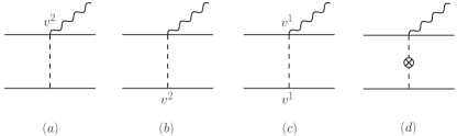
Figure 2: One-graviton exchange with external $\bar{h}^{00}$ momentum.

The diagrams that contain the exchange of one potential graviton are shown in Fig. 2 and are composed by the couplings between the source action terms (105-110) and also the propagator (119) and its correction (120). Notice that we need not separate out all of the various terms that arise in the Feynman rules into different orders in the PN expansion as is done in the appendix. We also calculated covariantly vertices, as is done when calculating in the Post-Minkowskian (PM) expansion (see e.g. Cheung:2018wkq ), and then expand in $v$, as a calculational check. However, for pedagogical purposes we have separated Feynman rules into give orders in the PN expansion. The results from Fig. 2 is given by

$$T_{Fig2a}^{00}\left(t,\mathbf{k}\right) =\sum_{a\neq b}\frac{5}{2}\frac{Gm_{a}m_{b}}{r}\mathbf{v}_{a}^{2}e^{-i\mathbf{k}\cdot\mathbf{x}_{a}},$$ (16)

$$T_{Fig2b}^{00}\left(t,\mathbf{k}\right) =\sum_{a\neq b}\frac{3}{2}\frac{Gm_{a}m_{b}}{r}\mathbf{v}_{b}^{2}e^{-i\mathbf{k}\cdot\mathbf{x}_{a}},$$ (17)

$$T_{Fig2c}^{00}\left(t,\mathbf{k}\right) =-\sum_{a\neq b}4\frac{Gm_{a}m_{b}}{r}\mathbf{v}_{a}\cdot\mathbf{v}_{b}e^{-i\mathbf{k}\cdot\mathbf{x}_{a}},$$ (18)

$$T_{Fig2d}^{00}\left(t,\mathbf{k}\right) =\sum_{a\neq b}\frac{Gm_{a}m_{b}}{2r}\left(-\mathbf{a}_{b}^{i}\mathbf{r}^{i}+\mathbf{v}_{b}^{2}-\left(\mathbf{v}_{b}\cdot\mathbf{n}\right)^{2}\right)e^{-i\mathbf{k}\cdot\mathbf{x}_{a}}.$$ (19)

Leaving

$$\int d^{3}\mathbf{x}T_{Fig2a-2d}^{00}\left[\mathbf{x}^{i}\mathbf{x}^{j}\right]_{TF} =\sum_{a\neq b}\frac{Gm_{a}m_{b}}{2r}\left[\left(5\mathbf{v}_{a}^{2}+4\mathbf{v}_{b}^{2}-8\mathbf{v}_{a}\cdot\mathbf{v}_{b}-\mathbf{a}_{b}\cdot\mathbf{r}-\left(\mathbf{v}_{b}\cdot\mathbf{n}\right)^{2}\right)\mathbf{x}_{a}^{i}\mathbf{x}_{a}^{j}\right]_{TF}.$$ (20)

Note the implicit dependence on the indices $a,b$ in the quantities $\mathbf{r}=\mathbf{x}_{a}-\mathbf{x}_{b}$, $r=\left|\mathbf{r}\right|$ and $\mathbf{n}=\frac{\mathbf{r}}{r}$ inside the sum.

Figure 3: Diagrams with two potential gravitons coupled to $\bar{h}_{00}$.

The graphs in Fig. 3 are composed by the source terms (105-107) together with the vertices (121-125) and (120). Note that we multipole expand the denominators in $\mathbf{k}/\mathbf{q}\sim v$

$$\frac{1}{\mathbf{q}^{2}\left(\mathbf{q}+\mathbf{k}\right)^{2}} =\frac{1}{\mathbf{q}^{4}}-\frac{2\left(\mathbf{q}\cdot\mathbf{k}\right)}{\mathbf{q}^{6}}+\frac{4\left(\mathbf{q}\cdot\mathbf{k}\right)^{2}}{\mathbf{q}^{8}}+...,$$ (21)

In calculating the contributions to the mass quadrupole sourced by the temporal components of the pseudotensor at 2PN, we are allowed to drop terms depending on $\mathbf{k}^{2}$ in the expansion of the denominator, since those terms contribute to the trace part of the mass quadrupole, which is removed in the definition of the STF moment. The results are organized in orders of the radiation momentum, as it is shown below:

$$T_{Fig3a}^{00}\left(t,\mathbf{k}\right) =\sum_{a\neq b}\frac{Gm_{a}m_{b}}{4r}e^{-i\mathbf{k}\cdot\mathbf{x}_{a}}\left\{2\left(\mathbf{v}^{2}+\mathbf{a}\cdot\mathbf{r}-\dot{r}^{2}\right)+5\mathbf{v}_{a}\cdot\mathbf{v}_{b}-5\mathbf{v}_{a}\cdot\mathbf{n}\mathbf{v}_{b}\cdot\mathbf{n}\right.$$

$$+i\mathbf{k}^{i}\left[\left(\mathbf{v}^{2}+\mathbf{a}\cdot\mathbf{r}-\dot{r}^{2}+\frac{5}{2}\mathbf{v}_{a}\cdot\mathbf{v}_{b}-\frac{5}{2}\mathbf{v}_{a}\cdot\mathbf{n}\mathbf{v}_{b}\cdot\mathbf{n}\right)\mathbf{r}^{i}\right.$$

$$\left.+\left(\frac{1}{2}r\dot{r}+\frac{5}{2}\mathbf{v}_{b}\cdot\mathbf{r}\right)\mathbf{v}_{b}^{i}-\left(2r\dot{r}+\frac{5}{2}\mathbf{v}_{b}\cdot\mathbf{r}\right)\mathbf{v}_{a}^{i}-r^{2}\left(\mathbf{a}_{a}^{i}+\mathbf{a}_{b}^{i}\right)\right]$$

$$+\frac{1}{6}\mathbf{k}^{i}\mathbf{k}^{j}\left[-\left(2\mathbf{v}^{2}+5\mathbf{v}_{a}\cdot\mathbf{v}_{b}-2\dot{r}^{2}-5\mathbf{v}_{a}\cdot\mathbf{n}\mathbf{v}_{b}\cdot\mathbf{n}+2\mathbf{a}\cdot\mathbf{r}\right)\mathbf{r}^{i}\mathbf{r}^{j}\right.$$

$$+\left(4\mathbf{v}_{a}\cdot\mathbf{r}+\mathbf{v}_{b}\cdot\mathbf{r}\right)\mathbf{v}_{a}^{i}\mathbf{r}^{j}-\left(2\mathbf{v}_{a}\cdot\mathbf{r}+8\mathbf{v}_{b}\cdot\mathbf{r}\right)\mathbf{v}_{b}^{i}\mathbf{r}^{j}$$

$$\left.\left.+r^{2}\left(-4\mathbf{v}^{i}\mathbf{v}^{j}-7\mathbf{v}_{a}^{i}\mathbf{v}_{b}^{j}+2\mathbf{a}_{a}^{i}\mathbf{r}^{j}+4\mathbf{a}_{b}^{i}\mathbf{r}^{j}\right)\right]\right\}+O\left(\mathbf{k}^{3}\right)+...,$$ (22)

$$T_{Fig3b}^{00}\left(t,\mathbf{k}\right) =-\sum_{a\neq b}\frac{Gm_{a}m_{b}}{r}e^{-i\mathbf{k}\cdot\mathbf{x}_{a}}\left[\frac{7}{4}\mathbf{v}_{b}^{2}+\frac{3}{4}\mathbf{v}_{a}^{2}-\frac{i}{2}\mathbf{k}^{i}\mathbf{v}_{b}^{2}\mathbf{r}^{i}\right.$$

$$\left.+\frac{1}{2}\mathbf{k}^{i}\mathbf{k}^{j}\left(\frac{1}{2}\mathbf{v}_{b}^{2}\mathbf{r}^{i}\mathbf{r}^{j}+2\mathbf{r}^{2}\mathbf{v}_{b}^{i}\mathbf{v}_{b}^{j}\right)\right]+O\left(\mathbf{k}^{3}\right)+...,$$ (23)

$$T_{Fig3c}^{00}\left(t,\mathbf{k}\right) =\sum_{a\neq b}\frac{2Gm_{a}m_{b}}{r}e^{-i\mathbf{k}\cdot\mathbf{x}_{a}}\left(2\mathbf{v}_{a}\cdot\mathbf{v}_{b}+\mathbf{k}^{i}\mathbf{k}^{j}\mathbf{r}^{2}\mathbf{v}_{a}^{i}\mathbf{v}_{b}^{j}\right)+O\left(\mathbf{k}^{3}\right)+...,$$ (24)

$$T_{Fig3d}^{00}\left(t,\mathbf{k}\right) =-\sum_{a\neq b}\frac{2Gm_{a}m_{b}}{r}e^{-i\mathbf{k}\cdot\mathbf{x}_{a}}\left\{-\frac{i}{2}\mathbf{k}^{i}\left[2\mathbf{r}^{2}\mathbf{a}_{a}^{i}+2\mathbf{v}_{a}^{i}\left(\mathbf{v}_{b}\cdot\mathbf{r}+\mathbf{v}_{a}\cdot\mathbf{r}\right)\right]\right.$$

$$\left.-\frac{1}{2}\mathbf{k}^{i}\mathbf{k}^{j}\left[\mathbf{r}^{2}\left(\mathbf{v}_{a}^{i}\mathbf{v}_{a}^{j}-\mathbf{v}_{a}^{i}\mathbf{v}_{b}^{i}-\mathbf{r}^{j}\mathbf{a}_{a}^{i}\right)-\mathbf{v}_{a}^{i}\mathbf{r}^{j}\left(\mathbf{v}_{a}\cdot\mathbf{r}+\mathbf{v}_{b}\cdot\mathbf{r}\right)\right]\right\}+O\left(\mathbf{k}^{3}\right)+...,$$ (25)

$$T_{Fig3e}^{00}\left(t,\mathbf{k}\right) =-\sum_{a\neq b}\frac{Gm_{a}m_{b}}{4r}e^{-i\mathbf{k}\cdot\mathbf{x}_{a}}\left\{6\left(-\mathbf{a}_{b}\cdot\mathbf{r}+\mathbf{v}_{b}^{2}-\left(\mathbf{v}_{b}\cdot\mathbf{n}\right)^{2}\right)\right.$$

$$-\frac{3i}{2}\mathbf{k}^{i}\left[\left(\mathbf{a}_{b}\cdot\mathbf{r}-\mathbf{v}_{b}^{2}+\left(\mathbf{v}_{b}\cdot\mathbf{n}\right)^{2}\right)\mathbf{r}^{i}-2\mathbf{v}_{b}\cdot\mathbf{r}\mathbf{v}_{b}^{i}+\mathbf{r}^{2}\mathbf{a}_{b}^{i}\right]$$

$$-\frac{1}{2}\mathbf{k}^{i}\mathbf{k}^{j}\left[\left(-\mathbf{a}_{b}\cdot\mathbf{r}+\mathbf{v}_{b}^{2}-\left(\mathbf{v}_{b}\cdot\mathbf{n}\right)^{2}\right)\mathbf{r}^{i}\mathbf{r}^{j}+4\mathbf{v}_{b}\cdot\mathbf{r}\mathbf{v}_{b}^{i}\mathbf{r}^{j}\right.$$

$$\left.\left.-2\mathbf{r}^{2}\mathbf{a}_{b}^{i}\mathbf{r}^{j}+2\mathbf{r}^{2}\mathbf{v}_{b}^{i}\mathbf{v}_{b}^{j}\right]\right\}+O\left(\mathbf{k}^{3}\right)+...\cdot$$ (26)

Together, these quantities provide us with the following contribution,

$$\int d^{3}\mathbf{x}T_{Fig3a-3e}^{00}\left[\mathbf{x}^{i}\mathbf{x}^{j}\right]_{TF} =\sum_{a\neq b}\frac{Gm_{a}m_{b}}{12r}\left[\left(-2\mathbf{v}_{a}^{2}-35\mathbf{v}_{b}^{2}+26\mathbf{v}_{a}\cdot\mathbf{v}_{b}-10\mathbf{v}_{a}\cdot\mathbf{n}\mathbf{v}_{b}\cdot\mathbf{n}\right.\right.$$

$$\left.+3\left(\mathbf{v}_{a}\cdot\mathbf{n}\right)^{2}+12\left(\mathbf{v}_{b}\cdot\mathbf{n}\right)^{2}-4\dot{r}^{2}+\mathbf{a}_{a}\cdot\mathbf{r}+8\mathbf{a}_{b}\cdot\mathbf{r}\right)\mathbf{x}_{a}^{i}\mathbf{x}_{a}^{j}$$

$$+\left(\mathbf{v}_{a}^{2}+\mathbf{v}_{a}\cdot\mathbf{v}_{b}-5\mathbf{v}_{a}\cdot\mathbf{n}\mathbf{v}_{b}\cdot\mathbf{n}+3\left(\mathbf{v}_{a}\cdot\mathbf{n}\right)^{2}-2\dot{r}^{2}+\mathbf{a}_{a}\cdot\mathbf{r}\right)\mathbf{x}_{a}^{i}\mathbf{x}_{b}^{j}$$

$$+\left(\mathbf{v}_{a}\cdot\mathbf{r}+\mathbf{v}_{b}\cdot\mathbf{r}\right)\left(-20\mathbf{v}_{a}^{i}\mathbf{x}_{a}^{j}+26\mathbf{v}_{a}^{i}\mathbf{x}_{b}^{j}\right)$$

$$\left.+\mathbf{r}^{2}\left(2\mathbf{v}_{a}^{i}\mathbf{v}_{a}^{j}-\mathbf{v}_{a}^{i}\mathbf{v}_{b}^{j}-22\mathbf{a}_{a}^{i}\mathbf{x}_{a}^{j}-23\mathbf{a}_{a}^{i}\mathbf{x}_{b}^{j}\right)\right]_{STF}.$$ (27)

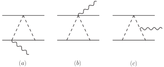
Figure 4: Two-potential-graviton exchange with external $\bar{h}^{00}$ momentum.

Contributions from Fig. 4 are composed of the source terms (105), (108), (112) and (113) and yield

$$T_{Fig4a}^{00}\left(t,\mathbf{k}\right) =\sum_{a\neq b}\frac{G^{2}m_{a}^{2}m_{b}}{r^{2}}e^{-i\mathbf{k}\cdot\mathbf{x}_{a}},$$ (28)

$$T_{Fig4b}^{00}\left(t,\mathbf{k}\right) =\sum_{a\neq b}\frac{3G^{2}m_{a}m_{b}^{2}}{2r^{2}}e^{-i\mathbf{k}\cdot\mathbf{x}_{a}},$$ (29)

$$T_{Fig4c}^{00}\left(t,\mathbf{k}\right) =-\sum_{a\neq b}\frac{3G^{2}m_{a}m_{b}m}{2r^{2}}e^{-i\mathbf{k}\cdot\mathbf{x}_{a}},$$ (30)

which gives us

$$\int d^{3}\mathbf{x}T_{Fig4a-4c}^{00}\left[\mathbf{x}^{i}\mathbf{x}^{j}\right]_{TF}=-\sum_{a\neq b}\frac{G^{2}m_{a}^{2}m_{b}}{2r^{2}}\left[\mathbf{x}_{a}^{i}\mathbf{x}_{a}^{j}\right]_{TF}.$$ (31)

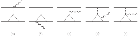
Figure 5: Three-potential-graviton exchange with external $\bar{h}^{00}$ momentum.

The diagrams illustrated in Fig. 5, are composed of the three-potential-graviton vertices (132-134) as well as the three-potential-one-radiation-graviton vertex (136-137) in composition with (105) and (108) contribute to $T_{2PN}^{00}$. These diagrams give:

$$T_{Fig5a}^{00}\left(t,\mathbf{k}\right) =-\sum_{a\neq b}\frac{G^{2}m_{a}m_{b}^{2}}{r^{2}}e^{-i\mathbf{k}\cdot\mathbf{x}_{a}},$$ (32)

$$T_{Fig5b}^{00}\left(t,\mathbf{k}\right) =-\sum_{a\neq b}\frac{2G^{2}m_{a}^{2}m_{b}}{r^{2}}e^{-i\mathbf{k}\cdot\mathbf{x}_{a}},$$ (33)

$$T_{Fig5c}^{00}\left(t,\mathbf{k}\right) =-\sum_{a\neq b}\frac{G^{2}m_{a}^{2}m_{b}}{r^{2}}e^{-i\mathbf{k}\cdot\mathbf{x}_{a}}\left(\frac{1}{2}-\frac{7}{2}i\mathbf{k}^{i}\mathbf{r}^{i}+\frac{5}{3}\mathbf{k}^{i}\mathbf{k}^{j}\mathbf{r}^{i}\mathbf{r}^{j}\right)+O\left(\mathbf{k}^{3}\right)+...,$$ (34)

$$T_{Fig5d}^{00}\left(t,\mathbf{k}\right) =\sum_{a\neq b}\frac{G^{2}m_{a}^{2}m_{b}}{r^{2}}e^{-i\mathbf{k}\cdot\mathbf{x}_{a}}\left(5-2i\mathbf{k}^{i}\mathbf{r}^{i}+\frac{2}{3}\mathbf{k}^{i}\mathbf{k}^{j}\mathbf{r}^{i}\mathbf{r}^{j}\right)+O\left(\mathbf{k}^{3}\right)+...,$$ (35)

$$T_{Fig5e}^{00}\left(t,\mathbf{k}\right) =-\sum_{a\neq b}\frac{G^{2}m_{a}m_{b}^{2}}{2r^{2}}e^{-i\mathbf{k}\cdot\mathbf{x}_{a}}.$$ (36)

Keeping terms to second order in the radiation momentum we have

$$\int d^{3}\mathbf{x}T_{Fig5a-5e}^{00}\left[\mathbf{x}^{i}\mathbf{x}^{j}\right]_{TF}=\sum_{a\neq b}\frac{G^{2}m_{a}m_{b}}{r^{2}}\left[\frac{3}{2}\left(m_{a}-m_{b}\right)\mathbf{x}_{a}^{i}\mathbf{x}_{a}^{j}-m_{a}\mathbf{x}_{a}^{i}\mathbf{x}_{b}^{j}+2m_{a}\mathbf{x}_{b}^{i}\mathbf{x}_{b}^{j}\right]_{TF}.$$ (37)

Summing the contributions (15), (20), (27), (31) and (37), the total contribution of $T_{2PN}^{00}$ to the mass quadrupole is

$$\int d^{3}\mathbf{x}T_{2PN}^{00}\left[\mathbf{x}^{i}\mathbf{x}^{j}\right]_{TF} =\sum_{a}\frac{3}{8}m_{a}\mathbf{v}_{a}^{4}\left[\mathbf{x}_{a}^{i}\mathbf{x}_{a}^{j}\right]_{TF}+\sum_{a\neq b}\frac{Gm_{a}m_{b}}{12r}\left[\left(28\mathbf{v}_{a}^{2}-11\mathbf{v}_{b}^{2}-22\mathbf{v}_{a}\cdot\mathbf{v}_{b}-10\mathbf{v}_{a}\cdot\mathbf{n}\mathbf{v}_{b}\cdot\mathbf{n}\right.\right.$$

$$\left.+3\left(\mathbf{v}_{a}\cdot\mathbf{n}\right)^{2}+6\left(\mathbf{v}_{b}\cdot\mathbf{n}\right)^{2}-4\dot{r}^{2}+\mathbf{a}_{a}\cdot\mathbf{r}+2\mathbf{a}_{b}\cdot\mathbf{r}+12\frac{Gm_{a}}{r}+6\frac{Gm_{b}}{r}\right)\mathbf{x}_{a}^{i}\mathbf{x}_{a}^{j}$$

$$+\left(\mathbf{v}_{a}^{2}+\mathbf{v}_{a}\cdot\mathbf{v}_{b}-5\mathbf{v}_{a}\cdot\mathbf{n}\mathbf{v}_{b}\cdot\mathbf{n}+3\left(\mathbf{v}_{a}\cdot\mathbf{n}\right)^{2}-2\dot{r}^{2}+\mathbf{a}_{a}\cdot\mathbf{r}-12\frac{Gm_{a}}{r}\right)\mathbf{x}_{a}^{i}\mathbf{x}_{b}^{j}$$

$$\left.+\left(\mathbf{v}_{a}\cdot\mathbf{r}+\mathbf{v}_{b}\cdot\mathbf{r}\right)\left(-20\mathbf{v}_{a}^{i}\mathbf{x}_{a}^{j}+26\mathbf{v}_{a}^{i}\mathbf{x}_{b}^{j}\right)+\mathbf{r}^{2}\left(2\mathbf{v}_{a}^{i}\mathbf{v}_{a}^{j}-\mathbf{v}_{a}^{i}\mathbf{v}_{b}^{j}-22\mathbf{a}_{a}^{i}\mathbf{x}_{a}^{j}-23\mathbf{a}_{a}^{i}\mathbf{x}_{b}^{j}\right)\right]_{STF}.$$ (38)

III.2 1PN correction to $T^{0i}$

The leading order $T^{0i}$ component was obtained in Goldberger:2009qd is

$$T_{0PN}^{0i}\left(t,\mathbf{k}\right)=\sum_{a}m_{a}\mathbf{v}_{a}^{i}e^{-i\mathbf{k}\cdot\mathbf{x}_{a}}.$$ (39)

The 1PN correction enter at $v^{3}$ and are shown in Fig. 6.

To extract the $T^{0i}$ contributions to the mass quadrupole moment, which is the third term in (10), the expansion of the denominator of vertices in Fig. 6c-6d has to be carried out to third order. In addition, $\mathbf{k}^{2}$ terms can not be dropped, since they contribute terms that cannot be included in the trace part of the quadrupole.

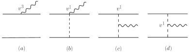
Figure 6: All diagrams that contribute to $T_{1PN}^{0i}$.

Comparing the diagrams illustrated in Fig.6, which are composed of (105,106,114,115) together with (119), (126) and (127) we find

$$T_{Fig6a}^{0l}\left(t,\mathbf{k}\right)=\sum_{a}\frac{m_{a}}{2}\mathbf{v}_{a}^{l}\mathbf{v}_{a}^{2}e^{-i\mathbf{k}\cdot\mathbf{x}_{a}},$$ (40)

$$T_{Fig6b}^{0l}\left(t,\mathbf{k}\right)=\sum_{a\neq b}\frac{Gm_{a}m_{b}}{r}\mathbf{v}_{a}^{l}e^{-i\mathbf{k}\cdot\mathbf{x}_{a}},$$ (41)

$$T_{Fig6c}^{0l}\left(t,\mathbf{k}\right) =\sum_{a\neq b}\frac{Gm_{a}m_{b}}{r}e^{-i\mathbf{k}\cdot\mathbf{x}_{a}}\left[-2\mathbf{v}_{a}^{l}+2i\mathbf{k}^{i}\left(\mathbf{v}_{a}^{i}\mathbf{r}^{l}-\mathbf{r}^{i}\mathbf{v}_{a}^{l}\right)+\mathbf{k}^{i}\mathbf{k}^{j}\left(\mathbf{r}^{i}\mathbf{r}^{j}\mathbf{v}_{a}^{l}-\mathbf{v}_{a}^{i}\mathbf{r}^{j}\mathbf{r}^{l}\right)\right.$$

$$\left.+\frac{i}{6}\mathbf{k}^{i}\mathbf{k}^{j}\mathbf{k}^{k}\left(\mathbf{r}^{2}\delta^{ij}\mathbf{v}_{a}^{k}\mathbf{r}^{l}-\mathbf{r}^{2}\delta^{il}\mathbf{v}_{a}^{j}\mathbf{r}^{k}-2\mathbf{v}_{a}^{i}\mathbf{r}^{j}\mathbf{r}^{k}\mathbf{r}^{l}+2\mathbf{r}^{i}\mathbf{r}^{j}\mathbf{r}^{k}\mathbf{v}_{a}^{l}\right)\right]+O\left(\mathbf{k}^{4}\right)+...,$$ (42)

$$T_{Fig6d}^{0l}\left(t,\mathbf{k}\right) =\sum_{a\neq b}\frac{Gm_{a}m_{b}}{4r}e^{-i\mathbf{k}\cdot\mathbf{x}_{a}}\left\{\mathbf{v}_{a}^{l}+\mathbf{v}_{b}^{l}-\frac{1}{r^{2}}\left(\mathbf{v}_{a}+\mathbf{v}_{b}\right)\cdot\mathbf{r}\mathbf{r}^{l}\right.$$

$$-\frac{i}{2}\mathbf{k}^{i}\left(3r\dot{r}\delta^{il}-\mathbf{r}^{i}\left(\mathbf{v}_{a}^{l}+\mathbf{v}_{b}^{l}\right)+\mathbf{v}^{i}\mathbf{r}^{l}+\frac{1}{r^{2}}\left(\mathbf{v}_{a}+\mathbf{v}_{b}\right)\cdot\mathbf{r}\mathbf{r}^{i}\mathbf{r}^{l}\right)$$

$$+\frac{1}{6}\mathbf{k}^{i}\mathbf{k}^{j}\left[-5\mathbf{r}^{2}\left(\mathbf{v}_{a}^{i}+\mathbf{v}_{b}^{i}\right)\delta^{jl}+\left(4\mathbf{v}_{a}\cdot\mathbf{r}-5\mathbf{v}_{b}\cdot\mathbf{r}\right)\mathbf{r}^{i}\delta^{jl}+\left(\mathbf{v}_{a}^{i}-2\mathbf{v}_{b}^{i}\right)\mathbf{r}^{j}\mathbf{r}^{l}\right.$$

$$\left.+\left(\mathbf{v}_{a}^{l}+\mathbf{v}_{b}^{l}\right)\left(\frac{1}{2}\delta^{ij}\mathbf{r}^{2}-\mathbf{r}^{i}\mathbf{r}^{j}\right)+\left(\mathbf{v}_{a}\cdot\mathbf{r}+\mathbf{v}_{b}\cdot\mathbf{r}\right)\left(\frac{1}{2}\delta^{ij}\mathbf{r}^{l}+\frac{1}{r^{2}}\mathbf{r}^{i}\mathbf{r}^{j}\mathbf{r}^{l}\right)\right]$$

$$-\frac{i}{24}\mathbf{k}^{i}\mathbf{k}^{j}\mathbf{k}^{k}\left[\delta^{kl}\left(6\mathbf{r}^{2}\mathbf{v}_{a}^{i}\mathbf{r}^{j}+14\mathbf{r}^{2}\mathbf{v}_{b}^{i}\mathbf{r}^{j}-5\mathbf{v}_{a}\cdot\mathbf{r}\mathbf{r}^{i}\mathbf{r}^{j}+7\mathbf{v}_{b}\cdot\mathbf{r}\mathbf{r}^{i}\mathbf{r}^{j}\right)\right.$$

$$+\delta^{ij}\mathbf{r}^{2}\left(3\delta^{kl}\mathbf{v}_{a}\cdot\mathbf{r}-3\delta^{kl}\mathbf{v}_{b}\cdot\mathbf{r}-\mathbf{r}^{k}\mathbf{v}_{b}^{l}-\mathbf{r}^{k}\mathbf{v}_{a}^{l}+\mathbf{v}_{a}^{k}\mathbf{r}^{l}-\mathbf{v}_{b}^{k}\mathbf{r}^{l}\right)-\delta^{ij}\left(\mathbf{v}_{a}\cdot\mathbf{r}+\mathbf{v}_{b}\cdot\mathbf{r}\right)\mathbf{r}^{k}\mathbf{r}^{l}$$

$$\left.\left.+\mathbf{r}^{i}\mathbf{r}^{j}\mathbf{r}^{k}\left(\mathbf{v}_{a}^{l}+\mathbf{v}_{b}^{l}\right)+\left(3\mathbf{v}_{b}^{i}-\mathbf{v}_{a}^{i}\right)\mathbf{r}^{j}\mathbf{r}^{k}\mathbf{r}^{l}-\frac{1}{r^{2}}\left(\mathbf{v}_{a}+\mathbf{v}_{b}\right)\cdot\mathbf{r}\mathbf{r}^{i}\mathbf{r}^{j}\mathbf{r}^{k}\mathbf{r}^{l}\right]\right\}+O\left(\mathbf{k}^{4}\right)+...\cdot$$ (43)

Expanding the exponentials up to the third order in the radiation momentum, we get

$$\int d^{3}\mathbf{x}\partial_{0}T_{1PN}^{0l}\mathbf{x}^{l}\left[\mathbf{x}^{i}\mathbf{x}^{j}\right]_{TF} =\sum_{a}\frac{d}{dt}\left[\frac{1}{2}m_{a}\mathbf{v}_{a}^{2}\mathbf{v}_{a}\cdot\mathbf{x}_{a}\mathbf{x}_{a}^{i}\mathbf{x}_{a}^{j}\right]_{TF}$$

$$+\sum_{a\neq b}\frac{d}{dt}\left\{\frac{Gm_{a}m_{b}}{12r}\left[\left(8\mathbf{r}^{2}-20\mathbf{r}\cdot\mathbf{x}_{b}\right)\mathbf{v}_{a}^{i}\mathbf{x}_{a}^{j}+\left(20\mathbf{r}^{2}-22\mathbf{r}\cdot\mathbf{x}_{b}\right)\mathbf{v}_{a}^{i}\mathbf{x}_{b}^{j}\right.\right.$$

$$+\left(22\mathbf{v}_{a}\cdot\mathbf{x}_{a}-30\mathbf{v}_{b}\cdot\mathbf{x}_{a}-8\mathbf{v}_{a}\cdot\mathbf{x}_{b}+8\mathbf{v}_{b}\cdot\mathbf{x}_{b}-\frac{2}{r^{2}}\left(\mathbf{v}_{a}+\mathbf{v}_{b}\right)\cdot\mathbf{r}\mathbf{r}\cdot\mathbf{x}_{b}\right)\mathbf{x}_{a}^{i}\mathbf{x}_{a}^{j}$$

$$\left.\left.+\left(9\mathbf{v}_{a}\cdot\mathbf{x}_{a}-7\mathbf{v}_{a}\cdot\mathbf{x}_{b}-\frac{1}{r^{2}}\left(\mathbf{v}_{a}+\mathbf{v}_{b}\right)\cdot\mathbf{r}\mathbf{r}\cdot\mathbf{x}_{b}\right)\mathbf{x}_{a}^{i}\mathbf{x}_{b}^{j}\right]\right\}_{STF}.$$ (44)

III.3 1PN correction to $T^{ii}$

The leading order $T^{ii}$ component obtained in Goldberger:2009qd has the form

$$T_{0PN}^{ii}\left(t,\mathbf{k}\right)=\left(\sum_{a}m_{a}\mathbf{v}_{a}^{2}-\sum_{a\neq b}\frac{Gm_{a}m_{b}}{2r}+O\left(\mathbf{k}\right)+...\right)e^{-i\mathbf{k}\cdot\mathbf{x}_{a}}.$$ (45)

Notice that, while $T_{0PN}^{0i}$ in (39) is down by $v^{1}$ relative to $T_{0PN}^{00}$ in (12), the leading order spatial component (45) is down by $v^{2}$ compared to $T_{0PN}^{00}$, this fixes the PN hierarchy among the components $T^{00}$, $T^{i0}$ and $T^{ij}$ of the pseudotensor.

To obtain $T_{1PN}^{ii}$ as well as its contributions to $I_{2PN}^{ij}$ we have to compute all diagrams that enter at $v^{4}$ with one $\bar{h}^{ii}$ external momentum. To compute the spatial component of the pseudotensor and to extract its contribution to the mass quadrupole moment we have to carry out the expansions up to the second order in the radiation momentum. $\mathbf{k}^{2}$ may be dropped as in section III.1.

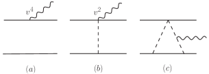
Figure 7: Diagrams with $\bar{h}^{ii}$ external momentum.

The diagrams illustrated in Fig. 7, involve (105, 112, 116, 117), (119) and (128) give

$$T_{Fig7a}^{ll}\left(t,\mathbf{k}\right) =\sum_{a}\frac{m_{a}}{2}\mathbf{v}_{a}^{4}e^{-i\mathbf{k}\cdot\mathbf{x}_{a}},$$ (46)

$$T_{Fig7b}^{ll}\left(t,\mathbf{k}\right) =\sum_{a\neq b}\frac{Gm_{a}m_{b}}{r}\mathbf{v}_{a}^{2}e^{-i\mathbf{k}\cdot\mathbf{x}_{a}},$$ (47)

$$T_{Fig7c}^{ll}\left(t,\mathbf{k}\right) =-\sum_{a\neq b}\frac{G^{2}m_{a}m_{b}m}{2r^{2}}e^{-i\mathbf{k}\cdot\mathbf{x}_{a}}.$$ (48)

It is straightforward to extract the contribution for the mass quadrupole moment by expanding the exponentials up to the second order in the radiation momentum,

$$\int d^{3}\mathbf{x}T_{Fig7a-7c}^{ll}\left[\mathbf{x}^{i}\mathbf{x}^{j}\right]_{TF}=\sum_{a}\frac{m_{a}}{2}\mathbf{v}_{a}^{4}\left[\mathbf{x}_{a}^{i}\mathbf{x}_{a}^{j}\right]_{TF}+\sum_{a\neq b}\frac{Gm_{a}m_{b}}{r}\left(\mathbf{v}_{a}^{2}-\frac{Gm}{2r}\right)\left[\mathbf{x}_{a}^{i}\mathbf{x}_{a}^{j}\right]_{TF}.$$ (49)

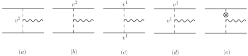
Figure 8: One potential graviton exchange with $\bar{h}^{ii}$ external momentum.

The computation of $T_{1PN}^{ii}$ follows from the diagrams shown in Fig. 8 which involve (105-107) and (119, 120, 128-131),

$$T_{Fig8a}^{ll}\left(t,\mathbf{k}\right) =\sum_{a\neq b}\frac{3Gm_{a}m_{b}}{4r}e^{-i\mathbf{k}\cdot\mathbf{x}_{a}}\left\{2\mathbf{v}^{2}+\mathbf{v}_{a}\cdot\mathbf{v}_{b}-2\dot{r}^{2}-\frac{1}{r^{2}}\mathbf{v}_{a}\cdot\mathbf{r}\mathbf{v}_{b}\cdot\mathbf{r}+2\mathbf{a}\cdot\mathbf{r}\right.$$

$$+\frac{i}{2}\mathbf{k}^{i}\left[\left(2\mathbf{v}^{2}+\mathbf{v}_{a}\cdot\mathbf{v}_{b}-2\dot{r}^{2}-\frac{1}{r^{2}}\mathbf{v}_{a}\cdot\mathbf{r}\mathbf{v}_{b}\cdot\mathbf{r}+2\mathbf{a}\cdot\mathbf{r}\right)\mathbf{r}^{i}\right.$$

$$\left.+\mathbf{v}_{b}^{i}\left(4\mathbf{v}_{b}\cdot\mathbf{r}-3\mathbf{v}_{a}\cdot\mathbf{r}\right)+\mathbf{v}_{a}^{i}\left(3\mathbf{v}_{b}\cdot\mathbf{r}-4\mathbf{v}_{a}\cdot\mathbf{r}\right)-2r^{2}\left(\mathbf{a}_{a}^{i}+\mathbf{a}_{b}^{i}\right)\right]$$

$$+\frac{1}{6}\mathbf{k}^{i}\mathbf{k}^{j}\left[\left(-2\mathbf{v}^{2}-\mathbf{v}_{a}\cdot\mathbf{v}_{b}-2\mathbf{a}\cdot\mathbf{r}+2\dot{r}^{2}+\frac{1}{r^{2}}\mathbf{v}_{a}\cdot\mathbf{r}\mathbf{v}_{b}\cdot\mathbf{r}\right)\mathbf{r}^{i}\mathbf{r}^{j}\right.$$

$$+\left(6\mathbf{v}_{a}\cdot\mathbf{r}-8\mathbf{v}_{b}\cdot\mathbf{r}\right)\mathbf{v}_{b}^{i}\mathbf{r}^{j}+\left(4\mathbf{v}_{a}\cdot\mathbf{r}-3\mathbf{v}_{b}\cdot\mathbf{r}\right)\mathbf{v}_{a}^{i}\mathbf{r}^{j}$$

$$\left.\left.+r^{2}\left(-4\mathbf{v}_{a}^{i}\mathbf{v}_{a}^{j}-3\mathbf{v}_{a}^{i}\mathbf{v}_{b}^{j}-4\mathbf{v}_{b}^{i}\mathbf{v}_{b}^{j}-4\mathbf{a}^{i}\mathbf{r}^{j}+6\mathbf{a}_{a}^{i}\mathbf{r}^{j}\right)\right]\right\}+O\left(\mathbf{k}^{3}\right)+...,$$ (50)

$$T_{Fig8b}^{ll}\left(t,\mathbf{k}\right)=\sum_{a\neq b}\frac{Gm_{a}m_{b}}{r}e^{-i\mathbf{k}\cdot\mathbf{x}_{a}}\left\{\frac{1}{4}\left(\mathbf{v}_{a}^{2}+\mathbf{v}_{b}^{2}\right)-i\mathbf{v}_{a}^{2}\mathbf{k}^{i}\mathbf{r}^{i}-\mathbf{k}^{i}\mathbf{k}^{j}\left(\mathbf{r}^{2}\mathbf{v}_{a}^{i}\mathbf{v}_{a}^{j}-\frac{1}{2}\mathbf{v}_{a}^{2}\mathbf{r}^{i}\mathbf{r}^{j}\right)\right\}+O\left(\mathbf{k}^{3}\right)+...,$$ (51)

$$T_{Fig8c}^{ll}\left(t,\mathbf{k}\right) =\sum_{a\neq b}\frac{Gm_{a}m_{b}}{2r}e^{-i\mathbf{k}\cdot\mathbf{x}_{a}}\left[-4\mathbf{v}_{a}\cdot\mathbf{v}_{b}-i\mathbf{k}^{i}\left(2\mathbf{v}_{a}\cdot\mathbf{v}_{b}\mathbf{r}^{i}+4\mathbf{v}_{a}\cdot\mathbf{r}\mathbf{v}_{b}^{i}-4\mathbf{v}_{b}\cdot\mathbf{r}\mathbf{v}_{a}^{i}\right)\right.$$

$$\left.+\mathbf{k}^{i}\mathbf{k}^{j}\left(2\mathbf{r}^{2}\mathbf{v}_{a}^{i}\mathbf{v}_{b}^{j}+\mathbf{v}_{a}\cdot\mathbf{v}_{b}\mathbf{r}^{i}\mathbf{r}^{j}-2\mathbf{v}_{b}\cdot\mathbf{r}\mathbf{v}_{a}^{i}\mathbf{r}^{j}+2\mathbf{v}_{a}\cdot\mathbf{r}\mathbf{v}_{b}^{i}\mathbf{r}^{j}\right)\right]+O\left(\mathbf{k}^{3}\right)+...,$$ (52)

$$T_{Fig8d}^{ll}\left(t,\mathbf{k}\right) =\sum_{a\neq b}\frac{Gm_{a}m_{b}}{r}e^{-i\mathbf{k}\cdot\mathbf{x_{a}}}\left\{-4\left(\mathbf{v}\cdot\mathbf{v}_{a}+\mathbf{a}_{a}\cdot\mathbf{r}-\frac{1}{r^{2}}\mathbf{v}\cdot\mathbf{r}\mathbf{v}_{a}\cdot\mathbf{r}\right)\right.$$

$$-2i\mathbf{k}^{i}\left[\mathbf{r}^{i}\left(\mathbf{v}\cdot\mathbf{v}_{a}+\mathbf{a}_{a}\cdot\mathbf{r}-\frac{\dot{r}}{r}\mathbf{v}_{a}\cdot\mathbf{r}\right)+\mathbf{v}_{a}\cdot\mathbf{r}\left(\mathbf{v}^{i}-2\mathbf{v}_{a}^{i}\right)\right]$$

$$+\frac{1}{3}\mathbf{k}^{i}\mathbf{k}^{j}\left[\mathbf{r}^{2}\left(\mathbf{v}^{i}\mathbf{v}_{a}^{j}+\mathbf{a}_{a}\mathbf{r}^{i}\right)+2\mathbf{r}^{i}\mathbf{r}^{j}\left(\mathbf{v}\cdot\mathbf{v}_{a}+\mathbf{a}_{a}\cdot\mathbf{r}\right)\right.$$

$$\left.\left.+r\dot{r}\mathbf{v}_{a}^{i}\mathbf{r}^{j}+2\mathbf{v}_{a}\cdot\mathbf{r}\left(2\mathbf{v}^{i}\mathbf{r}^{j}-3\mathbf{v}_{a}^{i}\mathbf{r}^{j}\right)-2\frac{\dot{r}}{r}\mathbf{v}_{a}\cdot\mathbf{r}\mathbf{r}^{i}\mathbf{r}^{j}\right]\right\}+O\left(\mathbf{k}^{3}\right)+...,$$ (53)

$$T_{Fig8e}^{ll}\left(t,\mathbf{k}\right) =-\sum_{a\neq b}\frac{Gm_{a}m_{b}}{4r}e^{-i\mathbf{k}\cdot\mathbf{x}_{a}}\left\{2\left(-\mathbf{a}_{b}\cdot\mathbf{r}+\mathbf{v}_{b}^{2}-\left(\mathbf{v}_{b}\cdot\mathbf{n}\right)^{2}\right)\right.$$

$$-\frac{i}{2}\mathbf{k}^{i}\left[\left(\mathbf{a}_{b}\cdot\mathbf{r}-\mathbf{v}_{b}^{2}+\left(\mathbf{v}_{b}\cdot\mathbf{n}\right)^{2}\right)\mathbf{r}^{i}-2\mathbf{v}_{b}\cdot\mathbf{r}\mathbf{v}_{b}^{i}+\mathbf{r}^{2}\mathbf{a}_{b}^{i}\right]$$

$$\left.+\frac{i^{2}}{6}\mathbf{k}^{i}\mathbf{k}^{j}\left[\left(-\mathbf{a}_{b}\cdot\mathbf{r}+\mathbf{v}_{b}^{2}-\left(\mathbf{v}_{b}\cdot\mathbf{n}\right)^{2}\right)\mathbf{r}^{i}\mathbf{r}^{j}+4\mathbf{v}_{b}\cdot\mathbf{r}\mathbf{v}_{b}^{i}\mathbf{r}^{j}-2\mathbf{r}^{2}\mathbf{a}_{b}^{i}\mathbf{r}^{j}+2\mathbf{r}^{2}\mathbf{v}_{b}^{i}\mathbf{v}_{b}^{j}\right]\right\}+O\left(\mathbf{k}^{3}\right)+...,$$ (54)

which provides us with

$$\int d^{3}\mathbf{x}T_{Fig8a-8e}^{ll}\left[\mathbf{x}^{i}\mathbf{x}^{j}\right]_{TF} =\sum_{a\neq b}\frac{Gm_{a}m_{b}}{12r}\left\{\left(10\mathbf{v}_{a}^{2}-17\mathbf{v}_{b}^{2}-10\mathbf{v}_{a}\cdot\mathbf{v}_{b}\right.\right.$$

$$\left.+5\left(\mathbf{v}_{a}\cdot\mathbf{n}\right)^{2}+2\mathbf{v}_{a}\cdot\mathbf{n}\mathbf{v}_{b}\cdot\mathbf{n}-8\left(\mathbf{v}_{b}\cdot\mathbf{n}\right)^{2}-5\mathbf{a}_{a}\cdot\mathbf{r}+8\mathbf{a}_{b}\cdot\mathbf{r}\right)\mathbf{x}_{a}^{i}\mathbf{x}_{a}^{j}$$

$$+\left(-5\mathbf{v}_{a}^{2}+7\mathbf{v}_{a}\cdot\mathbf{v}_{b}+5\left(\mathbf{v}_{a}\cdot\mathbf{n}\right)^{2}-7\mathbf{v}_{a}\cdot\mathbf{n}\mathbf{v}_{b}\cdot\mathbf{n}-5\mathbf{a}_{a}\cdot\mathbf{r}\right)\mathbf{x}_{a}^{i}\mathbf{x}_{b}^{j}$$

$$+\left(4\mathbf{v}_{a}\cdot\mathbf{r}-44\mathbf{v}_{b}\cdot\mathbf{r}\right)\mathbf{v}_{a}^{i}\mathbf{x}_{a}^{j}+\left(14\mathbf{v}_{a}\cdot\mathbf{r}-58\mathbf{v}_{b}\cdot\mathbf{r}\right)\mathbf{v}_{a}^{i}\mathbf{x}_{b}^{j}$$

$$\left.+r^{2}\left(38\mathbf{v}_{a}^{i}\mathbf{v}_{a}^{j}-7\mathbf{v}_{a}^{i}\mathbf{v}_{b}^{j}+14\mathbf{a}_{a}^{i}\mathbf{x}_{a}^{j}+19\mathbf{a}_{a}^{i}\mathbf{x}_{b}^{j}\right)\right\}_{STF}.$$ (55)

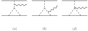
Figure 9: Three-potential-graviton exchange with $\bar{h}^{ii}$ external momentum.

Finally, the diagrams containing a three-potential-graviton exchange shown in Fig. 9 which involve (105), (135) and (138) give

$$T_{Fig9a}^{ll}\left(t,\mathbf{k}\right) =\sum_{a\neq b}\frac{G^{2}m_{a}^{2}m_{b}}{r^{2}}e^{-i\mathbf{k}\cdot\mathbf{x}_{a}}\left(-\frac{5}{2}+\frac{7}{2}i\mathbf{k}^{i}\mathbf{r}^{i}-\frac{4}{3}\mathbf{k}^{i}\mathbf{k}^{j}\mathbf{r}^{i}\mathbf{r}^{j}\right)+O\left(\mathbf{k}^{3}\right)+...$$ (56)

$$T_{Fig9b}^{ll}\left(t,\mathbf{k}\right) =\sum_{a\neq b}\frac{G^{2}m_{a}^{2}m_{b}}{r^{2}}e^{-i\mathbf{k}\cdot\mathbf{x}_{a}}\left(1-6i\mathbf{k}^{i}\mathbf{r}^{i}+\frac{7}{3}\mathbf{k}^{i}\mathbf{k}^{j}\mathbf{r}^{i}\mathbf{r}^{j}\right)+O\left(\mathbf{k}^{3}\right)+...$$ (57)

$$T_{Fig9c}^{ll}\left(t,\mathbf{k}\right) =\sum_{a\neq b}\frac{7G^{2}m_{a}m_{b}^{2}}{2r^{2}}e^{-i\mathbf{k}\cdot\mathbf{x}_{a}},$$ (58)

which leads to

$$\int d^{3}\mathbf{x}T_{Fig9a-9c}^{ll}\left[\mathbf{x}^{i}\mathbf{x}^{j}\right]_{TF}=\sum_{a\neq b}\frac{G^{2}m_{a}m_{b}}{r^{2}}\left[\frac{3}{2}m\mathbf{x}_{a}^{i}\mathbf{x}_{a}^{j}-m_{a}\mathbf{x}_{a}^{i}\mathbf{x}_{b}^{j}\right]_{STF}.$$ (59)

With this, we now write the total contribution of $T_{1PN}^{ll}$ to the mass quadrupole,

$$\int d^{3}\mathbf{x}T_{1PN}^{ll}\left[\mathbf{x}^{i}\mathbf{x}^{j}\right]_{TF} =\sum_{a}\frac{m_{a}}{2}\mathbf{v}_{a}^{4}\left[\mathbf{x}_{a}^{i}\mathbf{x}_{a}^{j}\right]_{TF}+\sum_{a\neq b}\frac{Gm_{a}m_{b}}{12r}\left\{\left(22\mathbf{v}_{a}^{2}-17\mathbf{v}_{b}^{2}-10\mathbf{v}_{a}\cdot\mathbf{v}_{b}\right.\right.$$

$$\left.+5\left(\mathbf{v}_{a}\cdot\mathbf{n}\right)^{2}+2\mathbf{v}_{a}\cdot\mathbf{n}\mathbf{v}_{b}\cdot\mathbf{n}-8\left(\mathbf{v}_{b}\cdot\mathbf{n}\right)^{2}-5\mathbf{a}_{a}\cdot\mathbf{r}+8\mathbf{a}_{b}\cdot\mathbf{r}+12\frac{Gm}{r}\right)\mathbf{x}_{a}^{i}\mathbf{x}_{a}^{j}$$

$$+\left(-5\mathbf{v}_{a}^{2}+7\mathbf{v}_{a}\cdot\mathbf{v}_{b}+5\left(\mathbf{v}_{a}\cdot\mathbf{n}\right)^{2}-7\mathbf{v}_{a}\cdot\mathbf{n}\mathbf{v}_{b}\cdot\mathbf{n}-5\mathbf{a}_{a}\cdot\mathbf{r}-12\frac{Gm_{a}}{r}\right)\mathbf{x}_{a}^{i}\mathbf{x}_{b}^{j}$$

$$+\left(4\mathbf{v}_{a}\cdot\mathbf{r}-44\mathbf{v}_{b}\cdot\mathbf{r}\right)\mathbf{v}_{a}^{i}\mathbf{x}_{a}^{j}+\left(14\mathbf{v}_{a}\cdot\mathbf{r}-58\mathbf{v}_{b}\cdot\mathbf{r}\right)\mathbf{v}_{a}^{i}\mathbf{x}_{b}^{j}$$

$$\left.+r^{2}\left(38\mathbf{v}_{a}^{i}\mathbf{v}_{a}^{j}-7\mathbf{v}_{a}^{i}\mathbf{v}_{b}^{j}+14\mathbf{a}_{a}^{i}\mathbf{x}_{a}^{j}+19\mathbf{a}_{a}^{i}\mathbf{x}_{b}^{j}\right)\right\}_{STF}.$$ (60)

IV Lower order stress-energy tensors

Although $T^{ij}_{0PN}$, $T^{ii}_{0PN}$ and $T^{00}_{1PN}$ have been computed before in Goldberger:2009qd , to write an expression for the mass quadrupole moment at 2PN order, we need to expand them in the radiation momentum to higher order and terms depending on $\mathbf{k}^{2}$ must be kept.

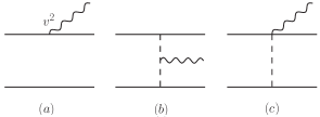
Figure 10: Diagrams (a) and (b) contribute to $T_{0PN}^{ij}$ when the external leg is $\bar{h}^{ij}\left(x\right)$, while diagrams (a), (b) and (c) contribute to $T_{1PN}^{00}$ when we consider $\bar{h}^{00}\left(x\right)$ as the external leg.

To obtain the sixth term of (10) we need diagrams in Fig. 10a-b. This gives us an expression for the leading order $T^{ij}$, as shown below:

$$T_{0PN}^{kl}\left(t,\mathbf{k}\right) =\sum_{a}m_{a}\mathbf{v}_{a}^{k}\mathbf{v}_{a}^{l}e^{-i\mathbf{k}\cdot\mathbf{x}_{a}}+\sum_{a\neq b}\frac{Gm_{a}m_{b}}{2r}e^{-i\mathbf{k}\cdot\mathbf{x}_{a}}\left\{-\frac{1}{r^{2}}\mathbf{r}^{k}\mathbf{r}^{l}-\frac{i}{2}\mathbf{k}^{i}\frac{1}{r^{2}}\mathbf{r}^{i}\mathbf{r}^{k}\mathbf{r}^{l}\right.$$

$$+\frac{1}{12}\mathbf{k}^{i}\mathbf{k}^{j}\left[10\mathbf{r}^{2}\left(\delta^{kl}\delta^{ij}-\delta^{ik}\delta^{jl}\right)+\delta^{kl}\mathbf{r}^{i}\mathbf{r}^{j}+\delta^{ij}\mathbf{r}^{k}\mathbf{r}^{l}-2\delta^{ik}\mathbf{r}^{j}\mathbf{r}^{l}+\frac{1}{r^{2}}2\mathbf{r}^{i}\mathbf{r}^{j}\mathbf{r}^{k}\mathbf{r}^{l}\right]$$

$$-\frac{i}{24}\mathbf{k}^{i}\mathbf{k}^{j}\mathbf{k}^{m}\left[\mathbf{r}^{2}\mathbf{r}^{m}\left(10\delta^{ik}\delta^{jl}-10\delta^{kl}\delta^{ij}\right)-\delta^{ij}\mathbf{r}^{m}\mathbf{r}^{k}\mathbf{r}^{l}+\mathbf{r}^{i}\mathbf{r}^{j}\left(2\delta^{mk}\mathbf{r}^{l}-\delta^{kl}\mathbf{r}^{m}-\frac{1}{r^{2}}\mathbf{r}^{m}\mathbf{r}^{k}\mathbf{r}^{l}\right)\right]$$

$$+\frac{1}{240}\mathbf{k}^{i}\mathbf{k}^{j}\mathbf{k}^{m}\mathbf{k}^{n}\left[\frac{16}{3}\mathbf{r}^{4}\delta^{mn}\left(\delta^{kl}\delta^{ij}-\delta^{ik}\delta^{jl}\right)+\mathbf{r}^{2}\delta^{ij}\delta^{mn}\mathbf{r}^{k}\mathbf{r}^{l}-2\mathbf{r}^{2}\delta^{mn}\delta^{ik}\mathbf{r}^{j}\mathbf{r}^{l}\right.$$

$$\left.\left.+\mathbf{r}^{m}\mathbf{r}^{n}\left(34\mathbf{r}^{2}\delta^{ik}\delta^{jl}-33\mathbf{r}^{2}\delta^{kl}\delta^{ij}-3\delta^{kl}\mathbf{r}^{i}\mathbf{r}^{j}+6\delta^{ik}\mathbf{r}^{j}\mathbf{r}^{l}-3\delta^{ij}\mathbf{r}^{k}\mathbf{r}^{l}-\frac{2}{r^{2}}\mathbf{r}^{i}\mathbf{r}^{j}\mathbf{r}^{k}\mathbf{r}^{l}\right)\right]\right\}+O\left(\mathbf{k}^{5}\right)+...$$ (61)

The first term in the expression above is related to Fig.10a, which comes from the simple source action term $-\sum\frac{m_{a}}{2m_{pl}}\int dt_{a}\mathbf{v}_{a}^{i}\mathbf{v}_{a}^{j}\overline{h}^{ij}\left(x_{a}\right).$ The other terms come from Fig. 10b, which is composed of (105) and (121) by considering,

$$F^{\left\langle H^{00}H^{00}\right\rangle}\left[q,k,\bar{h}^{ij}\right]=\bar{h}^{ij}\left[-\frac{1}{2}\mathbf{q}^{i}\mathbf{q}^{j}-\frac{1}{2}\mathbf{q}^{i}\mathbf{k}^{j}-\frac{1}{2}\mathbf{k}^{i}\mathbf{k}^{j}+\delta^{ij}\left(\frac{1}{4}\mathbf{q}^{2}+\frac{1}{4}\mathbf{k}\cdot\mathbf{q}+\frac{1}{2}\mathbf{k}^{2}\right)\right].$$ (62)

where $F^{\left\langle H^{00}H^{00}\right\rangle}$ is defined in (126).

Now, expanding the exponentials up to the fourth order in the radiation momentum, we extract the contribution

$$\int d^{3}\mathbf{x}\partial_{0}^{2}T_{0PN}^{kl}\mathbf{x}^{k}\mathbf{x}^{l}\left[\mathbf{x}^{i}\mathbf{x}^{j}\right]_{TF} =\frac{d^{2}}{dt^{2}}\left[\sum_{a}m_{a}\left(\mathbf{v}_{a}\cdot\mathbf{x}_{a}\right)^{2}\mathbf{x}_{a}^{i}\mathbf{x}_{a}^{j}\right]_{TF}$$

$$+\frac{d^{2}}{dt^{2}}\left\{\sum_{a\neq b}\frac{Gm_{a}m_{b}}{6r}\left[\left(27\mathbf{r}^{2}+\mathbf{x}_{a}^{2}-2\mathbf{x}_{a}\cdot\mathbf{x}_{b}-\frac{2}{r^{2}}\mathbf{r}\cdot\mathbf{x}_{a}\mathbf{r}\cdot\mathbf{x}_{b}\right)\mathbf{x}_{a}^{i}\mathbf{x}_{a}^{j}\right.\right.$$

$$\left.\left.+\left(\frac{27}{2}\mathbf{r}^{2}+\mathbf{x}_{a}^{2}-\frac{1}{r^{2}}\left(\mathbf{r}\cdot\mathbf{x}_{a}\right)^{2}\right)\mathbf{x}_{a}^{i}\mathbf{x}_{b}^{j}\right]\right\}_{STF}.$$ (63)

Taking the trace of (61), we get

$$T_{0PN}^{ll}\left(t,\mathbf{k}\right) =\sum_{a}m_{a}\mathbf{v}_{a}^{2}e^{-i\mathbf{k}\cdot\mathbf{x}_{a}}+\sum_{a\neq b}\frac{Gm_{a}m_{b}}{2r}e^{-i\mathbf{k}\cdot\mathbf{x}_{a}}\left[-1-\frac{i}{2}\mathbf{k}^{i}\mathbf{r}^{i}+\frac{1}{4}\mathbf{k}^{i}\mathbf{k}^{j}\left(7\mathbf{r}^{2}\delta^{ij}+\mathbf{r}^{i}\mathbf{r}^{j}\right)\right.$$

$$+\frac{i}{24}\mathbf{k}^{i}\mathbf{k}^{j}\mathbf{k}^{m}\left(21\mathbf{r}^{2}\delta^{ij}\mathbf{r}^{m}+2\mathbf{r}^{i}\mathbf{r}^{j}\mathbf{r}^{m}\right)$$

$$\left.+\frac{1}{144}\mathbf{k}^{i}\mathbf{k}^{j}\mathbf{k}^{m}\mathbf{k}^{n}\left(7\mathbf{r}^{4}\delta^{ij}\delta^{mn}-42\mathbf{r}^{2}\delta^{ij}\mathbf{r}^{m}\mathbf{r}^{n}-3\mathbf{r}^{i}\mathbf{r}^{j}\mathbf{r}^{m}\mathbf{r}^{n}\right)\right]+O\left(\mathbf{k}^{5}\right)+...,$$ (64)

which contributes to the quadrupole in the form below:

$$\int d^{3}\mathbf{x}\partial_{0}^{2}T_{0PN}^{ll}\mathbf{x}^{2}\left[\mathbf{x}^{i}\mathbf{x}^{j}\right]_{TF} =\frac{d^{2}}{dt^{2}}\left[\sum_{a}m_{a}\mathbf{v}_{a}^{2}\mathbf{x}_{a}^{2}\mathbf{x}_{a}^{i}\mathbf{x}_{a}^{j}\right]_{TF}$$

$$+\frac{d^{2}}{dt^{2}}\left\{\sum_{a\neq b}\frac{Gm_{a}m_{b}}{12r}\left[\left(-104\mathbf{x}_{a}^{2}+196\mathbf{x}_{a}\cdot\mathbf{x}_{b}-98\mathbf{x}_{b}^{2}\right)\mathbf{x}_{a}^{i}\mathbf{x}_{a}^{j}-49\mathbf{r}^{2}\mathbf{x}_{a}^{i}\mathbf{x}_{b}^{j}\right]\right\}_{STF}.$$ (65)

To be able to compute the seventh contribution in (10), we need an expression for $T_{1PN}^{00}$ up to the fourth order in the radiation momentum. We regard the source action term $-\sum\frac{m_{a}}{4m_{pl}}\int dt_{a}\mathbf{v}_{a}^{2}\overline{h}^{00}\left(x_{a}\right)$ and also (119), (105), (108) and (122) to solve the diagrams at Fig. 10a-c. With this, we get an expression for $T_{1PN}^{00}$ and its contribution to the mass quadrupole at 2PN, respectively:

$$T_{1PN}^{00}\left(t,\mathbf{k}\right) =\sum_{a}\frac{1}{2}m_{a}\mathbf{v}_{a}^{2}e^{-i\mathbf{k}\cdot\mathbf{x}_{a}}+\sum_{a\neq b}\frac{Gm_{a}m_{b}}{r}e^{-i\mathbf{k}\cdot\mathbf{x}_{a}}\left[-\frac{1}{2}\right.$$

$$\left.-\frac{3}{8}\mathbf{k}^{2}r^{2}\left(1+\frac{i}{2}\mathbf{k}^{i}\mathbf{r}^{i}-\frac{1}{6}\mathbf{k}^{i}\mathbf{k}^{j}\mathbf{r}^{i}\mathbf{r}^{j}+\frac{r^{2}}{36}\mathbf{k}^{i}\mathbf{k}^{j}\delta^{ij}\right)\right]+O\left(\mathbf{k}^{5}\right)+...,$$ (66)

$$\int d^{3}\mathbf{x}\partial_{0}^{2}T_{1PN}^{00}\mathbf{x}^{2}\left[\mathbf{x}^{i}\mathbf{x}^{j}\right]_{TF} =\frac{d^{2}}{dt^{2}}\left\{\sum_{a}\frac{1}{2}m_{a}\mathbf{v}_{a}^{2}\mathbf{x}_{a}^{2}\left[\mathbf{x}_{a}^{i}\mathbf{x}_{a}^{j}\right]_{TF}\right\}$$

$$+\frac{d^{2}}{dt^{2}}\left\{\sum_{a\neq b}\frac{Gm_{a}m_{b}}{r}\left[\frac{7}{4}\mathbf{r}^{2}\left(2\mathbf{x}_{a}^{i}\mathbf{x}_{a}^{j}+\mathbf{x}_{a}^{i}\mathbf{x}_{b}^{j}\right)-\frac{1}{2}\mathbf{x}_{a}^{2}\mathbf{x}_{a}^{i}\mathbf{x}_{a}^{j}\right]_{STF}\right\}.$$ (67)

Moreover, considering the expansion up to the fifth and sixth orders in the radiation momentum at (39) and (12), respectively, in addition to taking time derivatives, we get

$$\int d^{3}\mathbf{x}\partial_{0}^{3}T_{0PN}^{0l}\mathbf{x}^{2}\mathbf{x}^{l}\left[\mathbf{x}^{i}\mathbf{x}^{j}\right]_{TF} =\frac{d^{3}}{dt^{3}}\left[\sum_{a}m_{a}\mathbf{v}_{a}\cdot\mathbf{x}_{a}\mathbf{x}_{a}^{2}\mathbf{x}_{a}^{i}\mathbf{x}_{a}^{j}\right]_{TF},$$ (68)

$$\int d^{3}\mathbf{x}\partial_{0}^{4}T_{0PN}^{00}\mathbf{x}^{4}\left[\mathbf{x}^{i}\mathbf{x}^{j}\right]_{TF} =\frac{d^{4}}{dt^{4}}\left[\sum_{a}m_{a}\mathbf{x}_{a}^{4}\mathbf{x}_{a}^{i}\mathbf{x}_{a}^{j}\right]_{TF}.$$ (69)

Before writing the final expression for the 2PN correction to the mass quadrupole moment, we still need to write the contribution of $I_{1PN}^{ij}\left(\mathbf{a}_{1PN}\right)$, which is given by the two terms

$$\left[\int d^{3}\mathbf{x}\partial_{0}T_{0PN}^{0l}\mathbf{x}^{l}\mathbf{x}^{i}\mathbf{x}^{j}\right]_{TF} \xrightarrow{2PN}\sum_{a}m_{a}\mathbf{a}_{1PNa}\cdot\mathbf{x}_{a}\left[\mathbf{x}_{a}^{i}\mathbf{x}_{a}^{j}\right]_{TF},$$ (70)

$$\left[\int d^{3}\mathbf{x}\partial_{0}^{2}T_{0PN}^{00}\mathbf{x}^{2}\mathbf{x}^{i}\mathbf{x}^{j}\right]_{TF} \xrightarrow{2PN}\sum_{a}2m_{a}\left[\mathbf{x}_{a}^{2}\mathbf{a}_{1PNa}^{i}\mathbf{x}_{a}^{j}+\mathbf{a}_{1PNa}\cdot\mathbf{x}_{a}\mathbf{x}_{a}^{i}\mathbf{x}_{a}^{j}\right]_{STF},$$ (71)

where the 1PN correction to the acceleration, for instance obtained in PhysRevD.86.044029 using the EFT framework, is given by

$$\mathbf{a}_{1PN(1)}^{i} = \frac{Gm_{2}}{2r^{2}}\left\{\mathbf{n}^{i}\left[\frac{2Gm}{r}-3\left(\mathbf{v}_{1}^{2}+\mathbf{v}_{2}^{2}\right)+7\left(\mathbf{v}_{1}\cdot\mathbf{v}_{2}\right)+3\left(\mathbf{v}_{1}\cdot\mathbf{n}\right)\left(\mathbf{v}_{2}\cdot\mathbf{n}\right)\right]\right.$$ (72)

$$-\mathbf{v}_{1}^{i}\left(\mathbf{v}_{2}\cdot\mathbf{n}\right)-\left(\mathbf{v}_{1}\cdot\mathbf{n}\right)\mathbf{v}_{2}^{i}+\dot{r}\left(6\mathbf{v}_{1}^{i}-7\mathbf{v}_{2}^{i}-\mathbf{n}^{i}\left(\mathbf{v}_{2}\cdot\mathbf{n}\right)\right)$$

$$\left.-6r\mathbf{a}_{1}^{i}+7r\mathbf{a}_{2}^{i}+\left(\mathbf{v}^{i}-\mathbf{n}^{i}\dot{r}\right)\left(\mathbf{v}_{2}\cdot\mathbf{n}\right)+r\mathbf{n}^{i}\left(\mathbf{a}_{2}\cdot\mathbf{n}\right)+\mathbf{n}^{i}\left(\mathbf{v}_{2}\cdot\left(\mathbf{v}-\mathbf{n}\dot{r}\right)\right)\right\}$$

$$-\frac{1}{2}\mathbf{a}_{1}^{i}\mathbf{v}_{1}^{2}-\mathbf{v}_{1}^{i}\left(\mathbf{v}_{1}\cdot\mathbf{a}_{1}\right).$$

V Consistency tests

Here we check the expressions for the components $T_{2PN}^{00}$, $T_{1PN}^{0i}$ and $T_{1PN}^{ll}$, which were obtained here for the first time in EFT approach with previous results derived using different methods.

The results presented in section III.1 allow us to write down an expression for the temporal component of the pseudotensor up to 2PN order,

$$T^{00}\left(t,\mathbf{k}\right) =e^{-i\mathbf{k}\cdot\mathbf{x}_{a}}\left\{\sum_{a}m_{a}\left(1+\frac{1}{2}\mathbf{v}_{a}^{2}+\frac{3}{8}\mathbf{v}_{a}^{4}\right)+\sum_{a\neq b}\frac{Gm_{a}m_{b}}{2r}\left\{-1+\mathbf{v}^{2}+\frac{7}{2}\mathbf{v}_{a}^{2}-\frac{5}{2}\mathbf{v}_{b}^{2}+\frac{5}{2}\mathbf{v}_{a}\cdot\mathbf{v}_{b}\right.\right.$$

$$-\frac{5}{2}\mathbf{v}_{a}\cdot\mathbf{n}\mathbf{v}_{b}\cdot\mathbf{n}+2\left(\mathbf{v}_{b}\cdot\mathbf{n}\right)^{2}-\dot{r}^{2}+\mathbf{a}\cdot\mathbf{r}+2\mathbf{a}_{b}\cdot\mathbf{r}+\frac{G}{r}\left(4m_{a}-3m_{b}\right)$$

$$+\frac{1}{2}i\mathbf{k}^{i}\left[\left(\mathbf{v}^{2}+\frac{1}{2}\mathbf{v}_{b}^{2}+\frac{5}{2}\mathbf{v}_{a}\cdot\mathbf{v}_{b}-\dot{r}^{2}-\frac{5}{2}\mathbf{v}_{a}\cdot\mathbf{n}\mathbf{v}_{b}\cdot\mathbf{n}+\frac{3}{2}\left(\mathbf{v}_{b}\cdot\mathbf{n}\right)^{2}+\mathbf{a}\cdot\mathbf{r}+\frac{3}{2}\mathbf{a}_{b}\cdot\mathbf{r}\right)\mathbf{r}^{i}\right.$$

$$\left.\left.\left.+\left(8\mathbf{v}_{a}\cdot\mathbf{r}+\frac{11}{2}\mathbf{v}_{b}\cdot\mathbf{r}-2r\dot{r}\right)\mathbf{v}_{a}^{i}+\left(\frac{9}{2}\mathbf{v}_{b}\cdot\mathbf{r}+\frac{1}{2}r\dot{r}\right)\mathbf{v}_{b}^{i}+r^{2}\left(7\mathbf{a}_{a}^{i}-2\mathbf{a}_{b}^{i}\right)+\frac{6Gm}{r}\right]\right\}+O\left(\mathbf{k}^{2}\right)+...\right\}.$$ (73)

We can use (11) to read off different contributions of $T^{00}$ to the dynamics of the binary system. For instance, at zeroth order in the radiation momentum, we can read off the mechanical energy of the system. It is straightforward to see in (73) that the leading order terms in the PN approximation reproduce the total mass of the two-body system, while the next-to-leading order terms provide us with the Newtonian energy. The terms that account for the next-to-next-to-leading order (2PN) correction to this pseudotensor, which were calculated in the section III.1 of this paper, give us the following contribution to the conserved energy,

$$E_{1PN} =\int d^{3}\mathbf{x}T_{2PN}^{00}\left(x\right)$$

$$=\frac{3}{8}\sum\limits_{a}m_{a}\mathbf{v}_{a}^{4}+\sum_{a\neq b}\frac{Gm_{a}m_{b}}{4r}\left[6\mathbf{v}_{a}^{2}-7\left(\mathbf{v}_{a}\cdot\mathbf{v}_{b}\right)-\left(\mathbf{v}_{a}\cdot\mathbf{n}\right)\left(\mathbf{v}_{b}\cdot\mathbf{n}\right)+\frac{Gm}{r}\right].$$ (74)

This result is equal to the first correction to the Newtonian energy presented in Eq. (205) of blanchet and can also be calculated computing the Hamiltonian function using the Lagrangian obtained by Einstein, Infeld and Hoffman in eih0 .

Regarding the 2PN terms in Eq. (73), we can read off the correction to the center of mass position

$$\mathbf{G}_{2PN} =\int d^{3}\mathbf{x}T_{2PN}^{00}\left(x\right)\mathbf{x}$$

$$=\frac{3}{8}\sum\limits_{a}m_{a}\mathbf{v}_{a}^{4}\mathbf{x}_{a}+\sum_{a\neq b}\frac{Gm_{a}m_{b}}{4r}\left\{\left[\frac{19}{2}\mathbf{v}_{a}^{2}-7\mathbf{v}_{a}\cdot\mathbf{v}_{b}-\frac{7}{2}\mathbf{v}_{b}^{2}-\mathbf{v}_{a}\cdot\mathbf{n}\mathbf{v}_{b}\cdot\mathbf{n}\right.\right.$$

$$\left.\left.-\frac{1}{2}\left(\mathbf{v}_{a}\cdot\mathbf{n}\right)^{2}+\frac{1}{2}\left(\mathbf{v}_{b}\cdot\mathbf{n}\right)^{2}-5\frac{Gm_{a}}{r}+7\frac{Gm_{b}}{r}\right]\mathbf{x}_{a}-7\left(\mathbf{v}_{a}\cdot\mathbf{r}+\mathbf{v}_{b}\cdot\mathbf{r}\right)\mathbf{v}_{a}\right\},$$ (75)

which agrees with the result presented in Eq. (B2c) of PhysRevD.97.044037 , where $\frac{d\mathbf{G}}{dt}=\mathbf{P}$, the total conserved linear momentum, such that the center of mass frame is defined by $\mathbf{G}=0$. By solving this equation iteratively, using the equations of motion to reduce the second time derivatives of the position, we get the 2PN correction to the center of mass frame,

$$\delta\mathbf{r}_{2PN} =\frac{\nu\delta m}{m}\left\{\mathbf{r}\left[\left(\frac{3}{8}-\frac{3\nu}{2}\right)\mathbf{v}^{4}+\frac{Gm}{r}\left(\left(\frac{19}{8}+\frac{3\nu}{2}\right)\mathbf{v}^{2}\right)\right.\right.$$

$$\left.\left.+\left(-\frac{1}{8}+\frac{3\nu}{4}\right)\dot{r}^{2}+\left(\frac{7}{4}-\frac{\nu}{2}\right)\frac{Gm}{r}\right]-\mathbf{v}\left[\frac{7}{4}Gm\dot{r}\right]\right\},$$ (76)

which agrees with (B4a), (B4b) and (B5b) of PhysRevD.97.044037 .

Let us now consider the results obtained in section III.2 to write down an expression for $T^{0l}$ up to 1PN order,

$$T^{0l}\left(t,\mathbf{k}\right) =e^{-i\mathbf{k}\cdot\mathbf{x}_{a}}\left\{\sum_{a}m_{a}\mathbf{v}_{a}^{l}\left(1+\frac{1}{2}\mathbf{v}_{a}^{2}\right)+\sum_{a\neq b}\frac{Gm_{a}m_{b}}{4r}\left[-3\mathbf{v}_{a}^{l}+\mathbf{v}_{b}^{l}-\frac{1}{r^{2}}\left(\mathbf{v}_{a}+\mathbf{v}_{b}\right)\cdot\mathbf{r}\mathbf{r}^{l}\right.\right.$$

$$\left.\left.-\frac{i}{2}\mathbf{k}^{i}\left(\mathbf{v}^{i}\mathbf{r}^{l}-16\mathbf{v}_{a}^{i}\mathbf{r}^{l}+15\mathbf{r}^{i}\mathbf{v}_{a}^{l}-\mathbf{r}^{i}\mathbf{v}_{b}^{l}+3r\dot{r}\delta^{il}+\frac{1}{r^{2}}\left(\mathbf{v}_{a}+\mathbf{v}_{b}\right)\cdot\mathbf{r}\mathbf{r}^{i}\mathbf{r}^{l}\right)\right]+O\left(\mathbf{k}^{2}\right)+...\right\}$$ (77)

Taking into account only terms of order zero in the radiation momentum, we obtain the 1PN correction to the linear momentum of the binary system,

$$\mathbf{P}_{1PN}=\int d^{3}\mathbf{x}T_{1PN}^{0l}\left(x\right) =-\left[\frac{Gm_{1}m_{2}}{2r^{3}}\left(\mathbf{v}_{1}+\mathbf{v}_{2}\right)\cdot\mathbf{r}\right]\mathbf{x}_{1}^{l}+\left[\frac{m_{1}}{2}\mathbf{v}_{1}^{2}-\frac{Gm_{1}m_{2}}{2r}\right]\mathbf{v}_{1}^{l}+1\leftrightarrow 2.$$ (78)

The result above agrees with Eq. (B1) and Eq. (B2b) of reference PhysRevD.97.044037 . Considering all linear terms in the radiation momentum in (77), we are able to obtain the 1PN correction to the angular momentum of the binary system,

$$\mathbf{L}_{1PN}^{i}=-\frac{1}{2}\epsilon^{ilk}\int d^{3}\mathbf{x}\left(T_{1PN}^{0l}\mathbf{x}^{k}-T_{1PN}^{0k}\mathbf{x}^{l}\right) =\frac{1}{2}\nu m\left(\mathbf{r}\times\mathbf{v}\right)^{i}\left[\left(1-3\nu\right)\mathbf{v}^{2}+\frac{Gm}{r}\left(6+2\nu\right)\right],$$ (79)

which agrees with Eq. (2.9b) of reference kidder .

Furthermore, considering the result obtained in section III.3, we provide an expression for $T^{ll}\left(t,\mathbf{k}\right)$ up to 1PN order:

$$T^{ll}\left(t,\mathbf{k}\right) =e^{-i\mathbf{k}\cdot\mathbf{x}_{a}}\left\{\sum_{a}m_{a}\mathbf{v}_{a}^{2}\left(1+\frac{1}{2}\mathbf{v}_{a}^{2}\right)+\sum_{a\neq b}\frac{Gm_{a}m_{b}}{4r}\left\{-2-5\mathbf{v}_{a}^{2}+5\mathbf{v}_{b}^{2}-\mathbf{v}_{a}\cdot\mathbf{v}_{b}-6\dot{r}^{2}\right.\right.$$

$$-3\mathbf{v}_{a}\cdot\mathbf{n}\mathbf{v}_{b}\cdot\mathbf{n}+2\left(\mathbf{v}_{b}\cdot\mathbf{n}\right)^{2}+16\dot{r}\mathbf{v}_{a}\cdot\mathbf{n}-10\mathbf{a}_{a}\cdot\mathbf{r}-4\mathbf{a}_{b}\cdot\mathbf{r}+\frac{G}{r}\left(-8m_{a}+12m_{b}\right)$$

$$+i\mathbf{k}^{i}\left[\mathbf{r}^{i}\left(-9\mathbf{v}_{a}^{2}+\frac{5}{2}\mathbf{v}_{b}^{2}-\frac{1}{2}\mathbf{v}_{a}\cdot\mathbf{v}_{b}-\frac{3}{2}\mathbf{v}_{a}\cdot\mathbf{n}\mathbf{v}_{b}\cdot\mathbf{n}+\frac{1}{2}\left(\mathbf{v}_{b}\cdot\mathbf{n}\right)^{2}\right.\right.$$

$$\left.-3\dot{r}^{2}+8\dot{r}\mathbf{v}_{a}\cdot\mathbf{n}-5\mathbf{a}_{a}\cdot\mathbf{r}-\frac{5}{2}\mathbf{a}_{b}\cdot\mathbf{r}-\frac{10Gm_{a}}{r}\right)+\left(2\mathbf{v}_{a}\cdot\mathbf{r}+\frac{25}{2}\mathbf{v}_{b}\cdot\mathbf{r}\right)\mathbf{v}_{a}^{i}$$

$$\left.\left.\left.+\left(-\frac{9}{2}\mathbf{v}_{a}\cdot\mathbf{r}+5\mathbf{v}_{b}\cdot\mathbf{r}\right)\mathbf{v}_{b}^{i}-\mathbf{r}^{2}\left(3\mathbf{a}_{a}^{i}+\frac{5}{2}\mathbf{a}_{b}^{i}\right)\right]\right\}+O\left(\mathbf{k}^{2}\right)+...\right\}.$$ (80)

We can use the moment relation

$$\int d^{3}\mathbf{x}T^{ll}=\frac{1}{2}\frac{d^{2}}{dt^{2}}\int d^{3}\mathbf{x}T^{00}\mathbf{x}^{2}.$$ (81)

to prove the self-consistency of our results. At leading order in the PN expansion, it is trivial to prove that this relation holds using (73) and (80), while at next-to-leading order more computation is required. From (80) we can read off up to 1PN,

$$\int d^{3}\mathbf{x}T^{ll}=\sum_{a}m_{a}\mathbf{v}_{a}^{2}\left(1+\frac{1}{2}\mathbf{v}_{a}^{2}\right)+\sum_{a\neq b}\frac{Gm_{a}m_{b}}{r}\left[-\frac{1}{2}-\frac{1}{4}\mathbf{v}_{a}\cdot\mathbf{v}_{b}+\frac{3}{2}\left(\mathbf{v}_{a}\cdot\mathbf{n}\right)^{2}-\frac{7}{4}\mathbf{v}_{a}\cdot\mathbf{n}\mathbf{v}_{b}\cdot\mathbf{n}+\frac{5}{2}\frac{Gm_{a}}{r}\right].$$ (82)

To check if the result above satisfies (81), we need a complete expression for $T^{00}\left(t,\mathbf{k}\right)$ up to 1PN order and which contains all terms up to the quadratic order in the radiation momentum. In other words, we cannot discard terms proportional to $\mathbf{k}^{2}$ as we did in section III.1, where we drppped these terms that would not contribute to the trace-free quadrupole moment. Therefore, the expression that we need for $T^{00}\left(t,\mathbf{k}\right)$ is the sum of (12) with (66), which provides us with the following result up to 1PN order:

$$\frac{1}{2}\frac{d^{2}}{dt^{2}}\int d^{3}\mathbf{x}T^{00}\mathbf{x}^{2}=\frac{1}{2}\frac{d^{2}}{dt^{2}}\left[\sum_{a}m_{a}\left(1+\frac{1}{2}\mathbf{v}_{a}^{2}\right)\mathbf{x}_{a}^{2}+\sum_{a\neq b}\frac{Gm_{a}m_{b}}{r}\left(-\frac{1}{2}\mathbf{x}_{a}^{2}+\frac{9}{4}r^{2}\right)\right].$$ (83)

At this point, it is straightforward to show that, after taking the second order time derivative and imposing the leading and next-to-leading order equations of motion that (81) holds, as we expected.

VI Mass quadrupole moment at 2PN order

We are now ready to sum the contributions (38), (44), (60), (63), (65), (67), (68), (69) and to write down the expression for the 2PN correction to the mass quadrupole moment in a general orbit,

$$I_{2PN}^{ij} =\sum_{a}m_{a}f_{1(a)}^{ij}+\sum_{a\neq b}\frac{Gm_{a}m_{b}}{r}f_{2(a,b)}^{ij}+\frac{d}{dt}\left[\sum_{a}m_{a}f_{3(a)}^{ij}+\sum_{a\neq b}\frac{Gm_{a}m_{b}}{r}f_{4(a,b)}^{ij}\right]$$

$$+\frac{d^{2}}{dt^{2}}\left[\sum_{a}m_{a}f_{5(a)}^{ij}+\sum_{a\neq b}\frac{Gm_{a}m_{b}}{r}f_{6(a,b)}^{ij}\right]+\frac{d^{3}}{dt^{3}}\left[\sum_{a}m_{a}f_{7(a)}^{ij}\right]+\frac{d^{4}}{dt^{4}}\left[\sum_{a}m_{a}f_{8(a)}^{ij}\right],$$ (84)

where we have defined the following quantities for convenience:

$$f_{1(a)}^{ij}\equiv\left[\frac{7}{8}\mathbf{v}_{a}^{4}\mathbf{x}_{a}^{i}\mathbf{x}_{a}^{j}+\frac{11}{21}\mathbf{x}_{a}^{2}\mathbf{a}_{1PNa}^{i}\mathbf{x}_{a}^{j}-\frac{17}{21}\mathbf{a}_{1PNa}\cdot\mathbf{x}_{a}\mathbf{x}_{a}^{i}\mathbf{x}_{a}^{j}\right]_{STF},$$ (85)

$$f_{2(a,b)}^{ij} \equiv\frac{1}{12}\left[\left(50\mathbf{v}_{a}^{2}-28\mathbf{v}_{b}^{2}-32\mathbf{v}_{a}\cdot\mathbf{v}_{b}-4\dot{r}^{2}-24\mathbf{v}_{a}\cdot\mathbf{n}\mathbf{v}_{b}\cdot\mathbf{n}\right.\right.$$

$$\left.+8\left(\mathbf{v}_{a}\cdot\mathbf{n}\right)^{2}+14\left(\mathbf{v}_{b}\cdot\mathbf{n}\right)^{2}-4\mathbf{a}_{a}\cdot\mathbf{r}+10\mathbf{a}_{b}\cdot\mathbf{r}+24\frac{Gm_{a}}{r}+18\frac{Gm_{b}}{r}\right)\mathbf{x}_{a}^{i}\mathbf{x}_{a}^{j}$$

$$+\left(-4\mathbf{v}_{a}^{2}+8\mathbf{v}_{a}\cdot\mathbf{v}_{b}-12\mathbf{v}_{a}\cdot\mathbf{n}\mathbf{v}_{b}\cdot\mathbf{n}+8\left(\mathbf{v}_{a}\cdot\mathbf{n}\right)^{2}-2\dot{r}^{2}-4\mathbf{a}_{a}\cdot\mathbf{r}-24\frac{Gm_{1}}{r}\right)\mathbf{x}_{a}^{i}\mathbf{x}_{b}^{j}$$

$$+\mathbf{v}_{a}^{i}\mathbf{x}_{a}^{j}\left(-16\mathbf{v}_{a}\cdot\mathbf{r}-64\mathbf{v}_{b}\cdot\mathbf{r}\right)+\mathbf{v}_{a}^{i}\mathbf{x}_{b}^{j}\left(40\mathbf{v}_{a}\cdot\mathbf{r}-32\mathbf{v}_{b}\cdot\mathbf{r}\right)$$

$$\left.+\mathbf{r}^{2}\left(40\mathbf{v}_{a}^{i}\mathbf{v}_{a}^{j}-8\mathbf{v}_{a}^{i}\mathbf{v}_{b}^{j}-8\mathbf{a}_{a}^{i}\mathbf{x}_{a}^{j}-4\mathbf{a}_{a}^{i}\mathbf{x}_{b}^{j}\right)\right]_{STF},$$ (86)

$$f_{3(a)}^{ij}\equiv-\frac{2}{3}\mathbf{v}_{a}^{2}\mathbf{v}_{a}\cdot\mathbf{x}_{a}\left[\mathbf{x}_{a}^{i}\mathbf{x}_{a}^{j}\right]_{TF},$$ (87)

$$f_{4(a,b)}^{ij} \equiv-\frac{1}{9}\left[\left(8\mathbf{r}^{2}-20\mathbf{r}\cdot\mathbf{x}_{b}\right)\mathbf{v}_{a}^{i}\mathbf{x}_{a}^{j}+\left(20\mathbf{r}^{2}-22\mathbf{r}\cdot\mathbf{x}_{b}\right)\mathbf{v}_{a}^{i}\mathbf{x}_{b}^{j}\right.$$

$$+\left(22\mathbf{v}_{a}\cdot\mathbf{x}_{a}-30\mathbf{v}_{b}\cdot\mathbf{x}_{a}-8\mathbf{v}_{a}\cdot\mathbf{x}_{b}+8\mathbf{v}_{b}\cdot\mathbf{x}_{b}-\frac{2}{r^{2}}\left(\mathbf{v}_{a}+\mathbf{v}_{b}\right)\cdot\mathbf{r}\mathbf{r}\cdot\mathbf{x}_{b}\right)\mathbf{x}_{a}^{i}\mathbf{x}_{a}^{j}$$

$$\left.+\left(9\mathbf{v}_{a}\cdot\mathbf{x}_{a}-7\mathbf{v}_{a}\cdot\mathbf{x}_{b}-\frac{1}{r^{2}}\left(\mathbf{v}_{a}+\mathbf{v}_{b}\right)\cdot\mathbf{r}\mathbf{r}\cdot\mathbf{x}_{b}\right)\mathbf{x}_{a}^{i}\mathbf{x}_{b}^{j}\right]_{STF},$$ (88)

$$f_{5(a)}^{ij}\equiv\left(\frac{1}{6}\left(\mathbf{v}_{a}\cdot\mathbf{x}_{a}\right)^{2}+\frac{19}{84}\mathbf{v}_{a}^{2}\mathbf{x}_{a}^{2}\right)\left[\mathbf{x}_{a}^{i}\mathbf{x}_{a}^{j}\right]_{TF},$$ (89)

$$f_{6(a,b)}^{ij} \equiv\left[\left(\frac{31}{42}\mathbf{x}_{a}^{2}-\frac{11}{6}\mathbf{x}_{a}\cdot\mathbf{x}_{b}+\frac{8}{9}\mathbf{x}_{b}^{2}-\frac{1}{18}\frac{1}{r^{2}}\mathbf{r}\cdot\mathbf{x}_{a}\mathbf{r}\cdot\mathbf{x}_{b}\right)\mathbf{x}_{a}^{i}\mathbf{x}_{a}^{j}\right.$$

$$\left.+\left(\frac{4}{9}\mathbf{r}^{2}+\frac{1}{36}\mathbf{x}_{a}^{2}-\frac{1}{36}\frac{1}{r^{2}}\left(\mathbf{r}\cdot\mathbf{x}_{a}\right)^{2}\right)\mathbf{x}_{a}^{i}\mathbf{x}_{b}^{j}\right]_{STF},$$ (90)

$$f_{7(a)}^{ij}\equiv-\frac{1}{7}\mathbf{v}_{a}\cdot\mathbf{x}_{a}\mathbf{x}_{a}^{2}\left[\mathbf{x}_{a}^{i}\mathbf{x}_{a}^{j}\right]_{TF},$$ (91)

$$f_{8(a)}^{ij}\equiv\frac{23}{1512}\mathbf{x}_{a}^{4}\left[\mathbf{x}_{a}^{i}\mathbf{x}_{a}^{j}\right]_{TF}.$$ (92)

With the exception of the accelerations in (85) which are of 1PN order, all other accelerations in $I_{2PN}^{ij}$ should be taken as the Newtonian acceleration.

In order to write the 2PN correction of the mass quadrupole moment in the center of mass frame, we must have in mind that the positions of the compact bodies in this frame are given by

$$\mathbf{x}_{1} =\frac{m_{2}}{m}\mathbf{r}+\delta\mathbf{r}_{1PN}+...,$$ (93)

$$\mathbf{x}_{2} =-\frac{m_{1}}{m}\mathbf{r}+\delta\mathbf{r}_{1PN}+...,$$ (94)

where $\delta\mathbf{r}_{1PN}$ accounts for the 1PN correction to the center of mass frame, which can be obtained following the procedure presented through (75) and (76) but this time using (66). Thus, the corrections to the center of frame necessary to write the 2PN mass quadrupole are

$$\delta\mathbf{r}_{1PN} =\frac{\nu\delta m}{2m}\mathbf{r}\left(\mathbf{v}^{2}-\frac{Gm}{r}\right),$$ (95)

$$\delta\mathbf{r}_{2PN} =\frac{\nu\delta m}{2m}\left\{\mathbf{r}\left[\left(\frac{3}{4}-3\nu\right)\mathbf{v}^{4}+\frac{Gm}{r}\left(\left(\frac{19}{4}+3\nu\right)\mathbf{v}^{2}\right)\right.\right.$$

$$\left.\left.+\left(-\frac{1}{4}+\frac{3\nu}{2}\right)\dot{r}^{2}+\left(\frac{7}{2}-\nu\right)\frac{Gm}{r}\right]-\mathbf{v}\left[\frac{7}{2}Gm\dot{r}\right]\right\}.$$ (96)

Applying (93) and (94) to (8) and (9), we obtain the following contributions at 2PN order:

$$I_{0PN+2PN}^{ij}=\frac{\nu^{2}\delta m^{2}}{4m}\left(\mathbf{v}^{4}-2\mathbf{v}^{2}\frac{Gm}{r}+\frac{G^{2}m^{2}}{r^{2}}\right)\left[\mathbf{r}^{i}\mathbf{r}^{j}\right]_{TF},$$ (97)

$$I_{1PN+1PN}^{ij} =\frac{\nu^{2}\delta m^{2}}{21m}\left\{\left[-29\mathbf{v}^{4}+\frac{Gm}{r}\left(41\mathbf{v}^{2}+\frac{17}{2}\dot{r}^{2}-12\frac{Gm}{r}\right)\right]\mathbf{r}^{i}\mathbf{r}^{j}\right.$$

$$\left.+\left(24\mathbf{v}^{2}-19\frac{Gm}{r}\right)r\dot{r}\mathbf{v}^{i}\mathbf{r}^{j}+\left(-22\mathbf{v}^{2}+22\frac{Gm}{r}\right)r^{2}\mathbf{v}^{i}\mathbf{v}^{j}\right\}_{STF}.$$ (98)

Adding these two contributions to (84) after applying (93) and (94), we finally obtain the expression for the 2PN correction to the mass quadrupole moment in the center of mass frame,

$$I_{2PN}^{ij} =m\nu\left\{\mathbf{r}^{i}\mathbf{r}^{j}\left[\frac{1}{252}\left(653-1906\nu+337\nu^{2}\right)\frac{G^{2}m^{2}}{r^{2}}+\frac{1}{756}\left(2021-5947\nu-4883\nu^{2}\right)\frac{Gm}{r}v^{2}\right.\right.$$

$$-\frac{1}{756}\left(131-907\nu+1273\nu^{2}\right)\frac{Gm}{r}\dot{r}^{2}+\frac{1}{504}\left(253-1835\nu+3545\nu^{2}\right)v^{4}$$

$$-r\dot{r}\mathbf{r}^{i}\mathbf{v}^{j}\left[\frac{1}{378}\left(1085-4057\nu-1463\nu^{2}\right)\frac{Gm}{r}+\frac{1}{63}\left(26-202\nu+418\nu^{2}\right)v^{2}\right]$$

$$\left.+\mathbf{v}^{i}\mathbf{v}^{j}\left[\frac{1}{189}\left(742-335\nu-985\nu^{2}\right)\frac{Gm}{r}+\frac{1}{126}\left(41-337\nu+733\nu^{2}\right)v^{2}+\frac{5}{63}\left(1-5\nu+5\nu^{2}\right)\dot{r}^{2}\right]\right\}_{STF}.$$ (99)

We can use the result above to compute, for instance, the 2PN correction to the power loss, whose expression in terms of the multipole moments is given by andirad2

$$P=-\frac{G}{5}\left\{I_{ij}^{(3)}I_{ij}^{(3)}-\frac{5}{189}I_{ijk}^{(4)}I_{ijk}^{(4)}+\frac{5}{9072}I_{ijkl}^{(5)}I_{ijkl}^{(5)}+\frac{16}{9}J_{ij}^{(3)}J_{ij}^{(3)}-\frac{5}{84}J_{ijk}^{(4)}J_{ijk}^{(4)}+...\right\}.$$ (100)

The expressions for these multipole moments below 2PN order are known and can be found for instance in Porto:2016pyg . Considering all terms which contribute to the power loss at 2PN order in the expression above, making use of (99) and the 2PN acceleration (152) obtained in the appendix B, we get

$$P_{EFT}^{2PN} =-\frac{8}{15}\frac{G^{3}m^{4}\nu^{2}}{r^{4}}\left\{\frac{2}{3}\left(-253+1026\nu-56\nu^{2}\right)\frac{G^{3}m^{3}}{r^{3}}+\left[\frac{1}{756}\left(245185+81828\nu+4368\nu^{2}\right)v^{2}\right.\right.$$

$$\left.-\frac{1}{252}\left(97247+9798\nu+5376\nu^{2}\right)\dot{r}^{2}\right]\frac{G^{2}m^{2}}{r^{2}}+\left[\frac{1}{21}\left(-4446+5237\nu-1393\nu^{2}\right)v^{4}\right.$$

$$\left.+\frac{1}{7}\left(4987-8513\nu+2165\nu^{2}\right)v^{2}\dot{r}^{2}-\frac{1}{63}\left(33510-60971\nu+14290\nu^{2}\right)\right]\frac{Gm}{r}$$

$$+\frac{1}{42}\left(1692-5497\nu+4430\nu^{2}\right)v^{6}-\frac{1}{14}\left(1719-10278\nu+6292\nu^{2}\right)v^{4}\dot{r}^{2}$$

$$\left.+\frac{1}{14}\left(2018-15207\nu+7572\nu^{2}\right)v^{2}\dot{r}^{4}-\frac{1}{42}\left(2501-20234\nu+8404\nu^{2}\right)\dot{r}^{6}\right\}.$$ (101)

At this point we can see that (99) and (101) seem to be in disagreement with the results presented at PhysRevD.54.4813 and PhysRevD.56.7708 where the Epstein-Wagoner formalism and multipolar post-Minkowskian approach of Blanchet, Damour, and Iyer (BDI) were used, respectively. For instance, the mass quadrupole moment presented in this paper and ones in the mentioned references differ by a factor of $-\frac{4G^{2}m^{2}}{r^{2}}\left[m\nu\mathbf{r}^{i}\mathbf{r}^{j}\right]_{TF}$. The power loss shown above and the energy fluxes at (6.13d) in PhysRevD.54.4813 and at (3.5d) in PhysRevD.56.7708 differ by a global minus sign, as well as by the numerical factors on terms depending on $\frac{G^{5}m^{6}\nu^{2}v^{2}}{r^{6}}$ and $\frac{G^{5}m^{6}\nu^{2}\dot{r}^{2}}{r^{6}}$. The difference in the global sign comes from the relation $P=-\frac{dE}{dt}$, which is actually a matter of convention on how the energy flux is defined. For this reason, we consider instead $\left|P\right|=\left|\frac{dE}{dt}\right|$ and compare the result for the power loss obtained here against the ones in the literature, and we find the following difference

$$P_{EFT}-\bar{P}=\frac{32}{5}\frac{G^{5}m^{6}\nu^{2}}{r^{6}}\left(4v^{2}-3\dot{r}^{2}\right),$$ (102)

where $\bar{P}$ is the modulus of the energy flux computed via the Epstein-Wagoner and BDI approaches .

Furthermore, the 2PN acceleration obtained in the appendix B is also different from the one presented in PhysRevD.56.7708 , which was computed via the BDI formalism. It turns out that these differences should not be a surprise since the gauge choice adopted here and in other formalisms are not the same: in the BDI and in the Epstein-Wagoner approaches the harmonic gauge is used, while in the EFT approach we use the linearized harmonic gauge (4), which depends on the background field metric. The different gauge choices for fixing the gravity action imply different coordinate systems. In fact, the difference between the mass quadrupole moments suggests a coordinate transformation of the form

$$\mathbf{r}_{EFT}\to\bar{\mathbf{r}}-\frac{2G^{2}m^{2}}{r^{2}}\bar{\mathbf{r}},$$ (103)

where $\bar{\mathbf{r}}$ is the coordinate used in the BDI and Epstein-Wagoner approaches. When this transformation is applied to the power loss (101), we can verify that

$$P_{EFT}\left(\bar{\mathbf{r}}\right)=\bar{P}.$$ (104)

An analogous comparison holds for the mass quadrupole moment and the 2PN acceleration, showing the agreement between our results and the literature. It should also be noticed that this coordinate transformation was already brought to attention in nrgr when the authors used NRGR to calculate the spacetime metric generated by a point mass at rest.

VII Final remarks

In this paper, we provided an independent computation of the 2PN correction to the mass quadrupole moment of a binary system of compact bodies moving in general orbits, using the EFT approach in the linearized harmonic gauge. We calculated high order corrections to the components of the pseudo-stress-energy tensor, which were used to obtain the mass quadrupole moment correction as well as the 1PN correction to the conserved energy and to the linear and angular momenta of the system and the 2PN correction to the center of mass frame. We used these quantities to perform tests that confirmed the consistency of our results within the EFT formalism itself and with results presented in the literature computed using different formalisms. Therefore, we not only extracted the contributions of the stress-energy pseudotensor to the 2PN correction to the mass quadrupole, but we provided the expressions for the components of the pseudotensor with higher order corrections that will be useful for future calculations on the dynamics of compact binary system.

We also calculated the 2PN correction to the equation of motion in the linearized harmonic gauge that was used, together with the mass quadrupole moment obtained in this paper, to write down the power loss due to the emission of gravitational waves. We thus compared our results against the literature and we showed that the 2PN correction to the mass quadrupole moment, to the relative acceleration of the two-body system and to the power loss obtained in this paper are in agreement with the results computed via the BDI and in the Epstein-Wagoner formalisms once a coordinate transformation is performed.

Although the 2PN correction to the mass quadrupole and to the equation of motion of compact binary systems obtained here were known in the literature, this derivation establishes the ground work for higher order calculations in the EFT formalism. Finally, these are the final missing ingredients necessary for the analysis of the radiation reaction of the binary system at the next-to-next-to-leading order in the EFT approach, which will be presented in a future paper.

VIII Acknowledgements

A.K.L., N.T.M, and Z.Y. are supported in part by the National Science Foundation under Grant No. PHY-1820760.

Appendix A

In this appendix we show the ingredients used to compute the components of the pseudotensor. We used the package xAct xact from Mathematica for the extraction of the vertices from the action.

Source terms

The source action terms needed to compute the contributions to $T_{2PN}^{00}$ are given below:

$$S^{\mathbf{v}^{0}} =-\sum_{a}\frac{m_{a}}{2m_{Pl}}\int dt_{a}H^{00}\left(x_{a}\right),$$ (105)

$$S^{\mathbf{v}^{1}} =\sum_{a}\frac{m_{a}}{m_{Pl}}\int dt_{a}\mathbf{v}_{a}^{i}H^{0i}\left(x_{a}\right),$$ (106)

$$S^{\mathbf{v}^{2}} =-\sum_{a}\frac{m_{a}}{2m_{Pl}}\int dt_{a}\left(\frac{\mathbf{v}_{a}^{2}}{2}H^{00}\left(x_{a}\right)+\mathbf{v}_{a}^{i}\mathbf{v}_{a}^{j}H^{ij}\left(x_{a}\right)\right),$$ (107)

$$S_{\bar{h}^{00}}^{\mathbf{v}^{0}} =\sum_{a}\frac{m_{a}}{4m_{Pl}^{2}}\int dt_{a}H^{00}\left(x_{a}\right)\bar{h}^{00}\left(x_{a}\right),$$ (108)

$$S_{\bar{h}^{00}}^{\mathbf{v}^{1}} =-\sum_{a}\frac{m_{a}}{2m_{Pl}^{2}}\int dt_{a}\mathbf{v}_{a}^{i}H^{0i}\left(x_{a}\right)\bar{h}^{00}\left(x_{a}\right),$$ (109)

$$S_{\bar{h}^{00}}^{\mathbf{v}^{2}} =\sum_{a}\frac{m_{a}}{8m_{Pl}^{2}}\int dt_{a}\left(3\mathbf{v}_{a}^{2}H^{00}\left(x_{a}\right)+2\mathbf{v}_{a}^{i}\mathbf{v}_{a}^{j}H^{ij}\left(x_{a}\right)\right)\bar{h}^{00}\left(x_{a}\right),$$ (110)

$$S_{\bar{h}^{00}}^{\mathbf{v}^{4}} =-\sum_{a}\frac{3m_{a}}{16m_{Pl}}\int dt_{a}\mathbf{v}_{a}^{4}\bar{h}^{00}\left(x_{a}\right),$$ (111)

$$S_{H^{2}}^{\mathbf{v}^{0}} =\sum_{a}\frac{m_{a}}{8m_{Pl}^{2}}\int dt_{a}H^{00}\left(x_{a}\right)H^{00}\left(x_{a}\right),$$ (112)

$$S_{H^{2}\bar{h}^{00}}^{\mathbf{v}^{0}} =-\sum_{a}\frac{3m_{a}}{16m_{Pl}^{3}}\int dt_{a}H^{00}\left(x_{a}\right)H^{00}\left(x_{a}\right)\bar{h}^{00}\left(x_{a}\right).$$ (113)

In addition, to write down the contributions for $T_{1PN}^{0i}$ we must to consider

$$S_{\bar{h}^{0i}}^{\mathbf{v}^{1}} =-\sum_{a}\frac{m_{a}}{2m_{Pl}^{2}}\int dt_{a}\mathbf{v}_{a}^{i}H^{00}\left(x_{a}\right)\bar{h}^{0i}\left(x_{a}\right),$$ (114)

$$S_{\bar{h}^{0i}}^{\mathbf{v}^{3}} =\sum_{a}\frac{m_{a}}{2m_{Pl}}\int dt\mathbf{v}_{a}^{2}\mathbf{v}_{a}^{i}\bar{h}^{0i}\left(x_{a}\right),$$ (115)

whereas for $T_{1PN}^{ll}$ the following terms are also necessary,

$$S_{\bar{h}^{ij}}^{\mathbf{v}^{2}} =\sum_{a}\frac{m_{a}}{4m_{pl}^{2}}\int dt_{a}\mathbf{v}_{a}^{i}\mathbf{v}_{a}^{j}H^{00}\left(x_{a}\right)\overline{h}^{ij}\left(x_{a}\right),$$ (116)

$$S_{\bar{h}^{ij}}^{\mathbf{v}^{4}} =-\sum_{a}\frac{m_{a}}{4m_{pl}}\int dt_{a}\mathbf{v}_{a}^{2}\mathbf{v}_{a}^{i}\mathbf{v}_{a}^{j}\overline{h}^{ij}\left(x_{a}\right).$$ (117)

Although all the sources terms above are conveniently expressed in position space, effectively we perform the partial Fourier transform

$$H^{\mu\nu}\left(t,\mathbf{q}\right)=\int d^{3}xH^{\mu\nu}\left(t,\mathbf{x}\right)e^{-i\mathbf{q}\cdot\mathbf{x}},$$ (118)

to carry out the Feynman diagrams in momentum space.

Vertices

From the EH action expanded in the radiation and potential fields and fixed with the background gauge, we obtain the propagator

$$\left\langle H_{\mu\nu}\left(t,\mathbf{q}\right)H_{\alpha\beta}\left(t^{\prime},\mathbf{q}^{\prime}\right)\right\rangle=-i\left(2\pi\right)^{3}P_{\mu\nu\alpha\beta}\delta\left(t-t^{\prime}\right)\delta^{3}\left(\mathbf{q}+\mathbf{q}^{\prime}\right)\frac{1}{\mathbf{q}^{2}},$$ (119)

as well as its correction

$$\left\langle H_{\mu\nu}\left(t,\mathbf{q}\right)H_{\alpha\beta}\left(t^{\prime},\mathbf{q}^{\prime}\right)\right\rangle_{v^{2}}=-i\left(2\pi\right)^{3}P_{\mu\nu\alpha\beta}\frac{d^{2}}{dtdt^{\prime}}\delta\left(t-t^{\prime}\right)\delta^{3}\left(\mathbf{q}+\mathbf{q}^{\prime}\right)\frac{1}{\mathbf{q}^{4}}.$$ (120)

The two-potential-one-radiation vertex regarded inside the momentum integrals of the internal potential momenta coupled to the particles has the form

$$\int\frac{d^{3}\mathbf{q}}{\left(2\pi\right)^{3}}\int\frac{d^{3}\mathbf{q}^{\prime}}{\left(2\pi\right)^{3}}e^{-i\mathbf{q}\cdot\mathbf{x}_{1}}e^{-i\mathbf{q}^{\prime}\cdot\mathbf{x}_{2}}\left\langle iS_{\bar{h}H^{2}}\right\rangle=-\frac{i}{m_{Pl}}\delta\left(t-t^{\prime}\right)\int\frac{d^{3}\mathbf{q}}{\left(2\pi\right)^{3}}e^{-i\mathbf{q}\cdot\mathbf{x}}\frac{F\left[q,k,\bar{h}\right]}{\mathbf{q}^{2}\left(\mathbf{q}+\mathbf{k}\right)^{2}},$$ (121)

for which the different contractions necessary to write down the contributions to $T_{2PN}^{00}$ are

$$F^{\left\langle H^{00}H^{00}\right\rangle}\left[q,k,\bar{h}^{00}\right] =\bar{h}^{00}\left[\frac{3}{4}\left(\mathbf{q}^{2}+\mathbf{k}\cdot\mathbf{q}\right)-\frac{5}{4}q_{0}^{2}-\frac{5}{4}k_{0}q_{0}-\frac{1}{2}k_{0}^{2}\right],$$ (122)

$$F^{\left\langle\mathbf{v}_{1}^{k}H^{0k}H^{00}\right\rangle}\left[q,k,\bar{h}^{00}\right] =\bar{h}^{00}\mathbf{v}_{1}^{k}\left[-\mathbf{q}^{k}\left(q_{0}+\frac{1}{2}k_{0}\right)\right],$$ (123)

$$F^{\left\langle\mathbf{v}_{1}^{k}\mathbf{v}_{1}^{l}H^{kl}H^{00}\right\rangle}\left[q,k,\bar{h}^{00}\right] =\bar{h}^{00}\mathbf{v}_{1}^{k}\mathbf{v}_{1}^{l}\left[\frac{1}{4}\delta^{kl}\left(\mathbf{q}^{2}+3\mathbf{k}\cdot\mathbf{q}\right)-\frac{1}{2}\mathbf{k}^{k}\mathbf{k}^{l}\right],$$ (124)

$$F^{\left\langle\mathbf{v}_{1}^{k}H^{0k}H^{0l}\mathbf{v}_{2}^{l}\right\rangle}\left[q,k,\bar{h}^{00}\right] =\bar{h}^{00}\mathbf{v}_{1}^{k}\mathbf{v}_{2}^{l}\left[-\frac{1}{4}\delta^{kl}\left(\mathbf{q}^{2}+\mathbf{k}\cdot\mathbf{q}\right)+\frac{1}{4}\mathbf{k}^{k}\mathbf{k}^{l}\right].$$ (125)

On the other hand, to compute the contributions to $T_{1PN}^{0i}$, the contractions required are

$$F^{\left\langle H^{00}H^{00}\right\rangle}\left[q,k,\bar{h}^{0i}\right] =\bar{h}^{0i}\left[q_{0}\left(\mathbf{q}^{i}+\frac{1}{2}\mathbf{k}^{i}\right)+k_{0}\left(\frac{1}{2}\mathbf{q}^{i}+\mathbf{k}^{i}\right)\right],$$ (126)

$$F^{\left\langle\mathbf{v}_{1}^{k}H^{0k}H^{00}\right\rangle}\left[q,k,\bar{h}^{0i}\right] =\bar{h}^{0i}\mathbf{v}_{1}^{k}\left[-\delta^{ik}\left(\frac{1}{2}\mathbf{q}^{2}+\mathbf{k}\cdot\mathbf{q}\right)+\mathbf{q}^{i}\mathbf{k}^{k}+\frac{1}{2}\mathbf{k}^{i}\mathbf{k}^{k}\right],$$ (127)

whereas for $T_{1PN}^{ll}$ we need

$$F^{\left\langle H^{00}H^{00}\right\rangle}\left[q,k,\bar{h}^{ll}\right] =\bar{h}^{ll}\left[\frac{1}{4}\mathbf{q}^{2}+\frac{1}{4}\mathbf{k}\cdot\mathbf{q}-\frac{3}{4}\left(q_{0}^{2}+k_{0}q_{0}+2k_{0}^{2}\right)\right],$$ (128)

$$F^{\left\langle\mathbf{v}_{1}^{k}H^{0k}H^{00}\right\rangle}\left[q,k,\bar{h}^{ll}\right] =\bar{h}^{ll}\mathbf{v}_{1}^{k}\left[-k_{0}\left(\mathbf{q}^{k}+\frac{1}{2}\mathbf{k}^{k}\right)\right],$$ (129)

$$F^{\left\langle\mathbf{v}_{1}^{k}\mathbf{v}_{1}^{l}H^{kl}H^{00}\right\rangle}\left[q,k,\bar{h}^{ll}\right] =\bar{h}^{ll}\mathbf{v}_{1}^{k}\mathbf{v}_{1}^{l}\left[\delta^{kl}\left(-\frac{1}{4}\mathbf{q}^{2}+\frac{1}{4}\mathbf{k}\cdot\mathbf{q}\right)-\frac{1}{2}\mathbf{k}^{k}\mathbf{k}^{l}\right],$$ (130)

$$F^{\left\langle\mathbf{v}_{1}^{k}H^{0k}H^{0l}\mathbf{v}_{2}^{l}\right\rangle}\left[q,k,\bar{h}^{ll}\right] =\bar{h}^{ll}\mathbf{v}_{1}^{k}\mathbf{v}_{2}^{l}\left[\frac{1}{4}\delta^{kl}\left(\mathbf{q}^{2}+\mathbf{k}\cdot\mathbf{q}\right)-\frac{1}{2}\mathbf{q}^{l}\mathbf{k}^{k}+\frac{1}{2}\mathbf{q}^{k}\mathbf{k}^{l}+\frac{1}{4}\mathbf{k}^{k}\mathbf{k}^{l}\right].$$ (131)

The three-graviton vertex, in turn, comes naturally in a simple form even not integrated on the internal momenta:

$$\left\langle H_{\mathbf{q}_{1}}^{00}H_{\mathbf{q}_{2}}^{00}H_{\mathbf{q}_{3}}^{00}\right\rangle =-\frac{\left(2\pi\right)^{3}}{4m_{Pl}}\delta\left(t_{2}-t_{1}\right)\delta\left(t_{3}-t_{1}\right)\delta^{3}\left(\bm{q}_{1}+\bm{q}_{2}+\bm{q}_{3}\right)\frac{\left(\bm{q}_{1}^{2}+\bm{q}_{2}^{2}+\bm{q}_{3}^{2}\right)}{\bm{q}_{1}^{2}\bm{q}_{2}^{2}\bm{q}_{3}^{2}}.$$ (132)

The composition of the three-potential-graviton vertex with two-potential-one-radiation-graviton vertex, after integrating in the third momentum, the integrand takes the form

$$\frac{F\left[\mathbf{q}_{1},\mathbf{q}_{2},\mathbf{k},\bar{h}\right]}{\mathbf{q}_{1}^{2}\mathbf{q}_{2}^{2}\left(\mathbf{q}_{1}+\mathbf{k}\right)^{2}\left(\mathbf{q}_{1}+\mathbf{q}_{2}+\mathbf{k}\right)^{2}},$$ (133)

in which the numerators for the contractions needed to compute the contributions for $T_{2PN}^{00}$ and $T_{1PN}^{ll}$ are, respectively,

$$F^{\left\langle H^{00}H^{00}H^{00}\right\rangle}\left[\mathbf{q}_{1},\mathbf{q}_{2},\mathbf{k},\bar{h}^{00}\right] =\frac{1}{4}\bar{h}_{00}\left[\mathbf{q}_{1}^{4}+\frac{5}{2}\mathbf{q}_{1}^{2}\left(\mathbf{q}_{1}\cdot\mathbf{q}_{2}\right)+\frac{5}{2}\mathbf{q}_{1}^{2}\mathbf{q}_{2}^{2}+\left(\mathbf{q}_{1}+\mathbf{q}_{2}\right)^{2}\left(\mathbf{q}_{1}\cdot\mathbf{k}\right)\right.$$

$$\left.+\frac{5}{2}\mathbf{q}_{1}^{2}\left(\mathbf{q}_{2}\cdot\mathbf{k}\right)+3\left(\mathbf{q}_{1}\cdot\mathbf{k}\right)\left(\mathbf{q}_{2}\cdot\mathbf{k}\right)-\left(\mathbf{q}_{1}\cdot\mathbf{k}\right)^{2}+\left(\mathbf{q}_{2}\cdot\mathbf{k}\right)^{2}\right],$$ (134)

$$F^{\left\langle H^{00}H^{00}H^{00}\right\rangle}\left[\mathbf{q}_{1},\mathbf{q}_{2},\mathbf{k},\bar{h}^{ll}\right] =-\frac{\bar{h}^{ll}}{8}\left[2\mathbf{q}_{1}^{4}-\mathbf{q}_{1}^{2}\mathbf{q}_{1}\cdot\mathbf{q}_{2}+10\mathbf{q}_{1}^{2}\mathbf{q}_{1}\cdot\mathbf{k}+10\left(\mathbf{q}_{1}\cdot\mathbf{k}\right)^{2}-\mathbf{q}_{1}^{2}\mathbf{q}_{2}^{2}\right.$$

$$\left.-\mathbf{q}_{1}^{2}\mathbf{q}_{2}\cdot\mathbf{k}-2\left(\mathbf{q}_{1}\cdot\mathbf{k}\right)\left(\mathbf{q}_{2}\cdot\mathbf{k}\right)-2\left(\mathbf{q}_{2}\cdot\mathbf{k}\right)^{2}\right].$$ (135)

The three-potential-one-radiation-graviton vertex integrated in the internal momenta can be expressed in this way:

$$\prod_{i=1}^{3}\int\frac{d^{3}\mathbf{q}_{i}}{\left(2\pi\right)^{9}}e^{i\mathbf{q}_{i}\cdot\mathbf{x}_{i}}\left\langle iS_{\bar{h}H^{3}}\right\rangle=-\frac{1}{m_{Pl}^{2}}\delta\left(t_{2}-t_{1}\right)\delta\left(t_{3}-t_{1}\right)\int\frac{d^{3}\mathbf{q}_{2}}{\left(2\pi\right)^{3}}\int\frac{d^{3}\mathbf{q}_{3}}{\left(2\pi\right)^{3}}\frac{e^{i\left(\mathbf{q}_{2}+\mathbf{q}_{3}\right)\cdot\mathbf{x}}F\left[\mathbf{q}_{2},\mathbf{q}_{3},\mathbf{k},\bar{h}\right]}{\mathbf{q}_{2}^{2}\mathbf{q}_{3}^{2}\left(\mathbf{q}_{2}+\mathbf{q}_{3}+\mathbf{k}\right)^{2}},$$ (136)

where we have chosen to integrate on $\mathbf{q}_{1}$, for instance coupled to particle 1, and leaving the momenta $\mathbf{q}_{2}$ and $\mathbf{q}_{3}$, both coupled to particle 2, to be integrated in the process of solving the diagrams. For this case, the contractions required to write down the contribution for $T_{2PN}^{00}$ and $T_{1PN}^{ll}$, respectively, are given by

$$F^{\left\langle H^{00}H^{00}H^{00}\right\rangle}\left[\mathbf{q}_{2},\mathbf{q}_{3},\mathbf{k},\bar{h}^{00}\right] =-\frac{1}{8}\bar{h}^{00}\left(\mathbf{q}_{2}^{2}+\mathbf{q}_{3}^{2}+\mathbf{q}_{2}\cdot\mathbf{q}_{3}+\mathbf{q}_{2}\cdot\mathbf{k}+\mathbf{q}_{3}\cdot\mathbf{k}\right),$$ (137)

$$F^{\left\langle H^{00}H^{00}H^{00}\right\rangle}\left[\mathbf{q}_{2},\mathbf{q}_{3},\mathbf{k},\bar{h}^{ll}\right] =-\frac{7}{8}\bar{h}^{ll}\left(\mathbf{q}_{2}^{2}+\mathbf{q}_{3}^{2}+\mathbf{q}_{2}\cdot\mathbf{q}_{3}+\mathbf{q}_{2}\cdot\mathbf{k}+\mathbf{q}_{3}\cdot\mathbf{k}\right).$$ (138)

Integrals

To solve integrals in the momentum space, it is helpful to use some general relations that can be obtained by using Feynman parameters Peskin:1995ev . If we consider a spacetime of $d$ dimensions, then for $D=d-1$ we have

$$\int\frac{d^{D}\mathbf{k}}{\left(2\pi\right)^{D}}\frac{e^{-i\mathbf{k}\cdot\mathbf{r}}}{\left(\mathbf{k}^{2}\right)^{a}} =\frac{1}{\left(4\pi\right)^{\frac{D}{2}}}\frac{\Gamma\left(\frac{D}{2}-a\right)}{\Gamma\left(a\right)}\left(\frac{r^{2}}{4}\right)^{a-\frac{D}{2}},$$ (139)

$$\int\frac{d^{D}\mathbf{k}}{\left(2\pi\right)^{D}}\frac{1}{\left[\mathbf{k}^{2}\right]^{a}\left[\left(\mathbf{k}-\mathbf{p}\right)^{2}\right]^{b}} =\frac{\left(\mathbf{p}^{2}\right)^{\frac{D}{2}-a-b}}{\left(4\pi\right)^{\frac{D}{2}}}\frac{\Gamma\left(a+b-\frac{D}{2}\right)}{\Gamma\left(a\right)\Gamma\left(b\right)}\frac{\Gamma\left(\frac{D}{2}-a\right)\Gamma\left(\frac{D}{2}-b\right)}{\Gamma\left(D-a-b\right)},$$ (140)

$$\int\frac{d^{D}\mathbf{k}}{\left(2\pi\right)^{D}}\frac{\mathbf{k}^{i}}{\left[\mathbf{k}^{2}\right]^{a}\left[\left(\mathbf{k}-\mathbf{p}\right)^{2}\right]^{b}} =\frac{\mathbf{p}^{i}\left(\mathbf{p}^{2}\right)^{\frac{D}{2}-a-b}}{\left(4\pi\right)^{\frac{D}{2}}}\frac{\Gamma\left(a+b-\frac{D}{2}\right)}{\Gamma\left(a\right)\Gamma\left(b\right)}\frac{\Gamma\left(\frac{D}{2}-a+1\right)\Gamma\left(\frac{D}{2}-b\right)}{\Gamma\left(D-a-b+1\right)},$$ (141)

$$\int\frac{d^{D}\mathbf{k}}{\left(2\pi\right)^{D}}\frac{\mathbf{k}^{i}\mathbf{k}^{j}}{\left[\mathbf{k}^{2}\right]^{a}\left[\left(\mathbf{k}-\mathbf{p}\right)^{2}\right]^{b}} =\frac{1}{\left(4\pi\right)^{\frac{D}{2}}}\frac{\left(\mathbf{p}^{2}\right)^{\frac{D}{2}-a-b}}{\Gamma\left(a\right)\Gamma\left(b\right)\Gamma\left(D-a-b+2\right)}$$

$$\times\left\{\frac{g^{ij}\mathbf{p}^{2}}{2}\Gamma\left(a+b-1-\frac{D}{2}\right)\Gamma\left(\frac{D}{2}-a+1\right)\Gamma\left(\frac{D}{2}-b+1\right)\right.$$

$$\left.+\mathbf{p}^{i}\mathbf{p}^{j}\Gamma\left(a+b-\frac{D}{2}\right)\Gamma\left(\frac{D}{2}-b\right)\Gamma\left(\frac{D}{2}-a+2\right)\right\}.$$ (142)

These integrals are especially important to solve diagrams that has a composition of the three-potential-graviton vertex with the two-potential-one-radiation vertex, where an analysis of the integrals in an arbitrary dimension $D$ is required to handle divergences.

Appendix B

In this appendix we present the result for the 2PN acceleration computed via the EFT approach in the linearized harmonic gauge.

To write down the equation of motion of the binary system at 2PN order, we need to obtain the Lagrangian by integrating out the potential modes of the gravitational fields in the action (2). Below the diagrams which contribute to the dynamics at 2PN order are presented.

Figure 11: Diagram with no graviton exchange.

The simplest contribution to the 2PN Lagrangian comes from the diagram show in Fig. 11, which gives the following contribution:

$$L_{Fig11}=\sum_{a}\frac{1}{16}m_{a}\mathbf{v}_{a}^{6}.$$ (143)

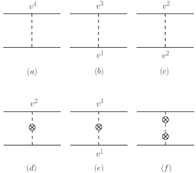
Figure 12: Diagrams with one-graviton exchange.

Next, we have the diagrams with one-graviton exchange illustrated in Fig. 12. Summing those diagrams together yields

$$L_{Fig12} =\sum_{a\neq b}\frac{Gm_{a}m_{b}}{16r^{3}}\left\{15r^{4}\mathbf{a}_{a}\cdot\mathbf{a}_{b}+r^{2}\left[14\mathbf{v}_{a}^{2}-20\mathbf{v}_{a}^{2}\mathbf{v}_{a}\cdot\mathbf{v}_{b}+2\left(\mathbf{v}_{a}\cdot\mathbf{v}_{b}\right)^{2}\right.\right.$$

$$\left.+3\mathbf{v}_{a}^{2}\mathbf{v}_{b}^{2}+2\mathbf{v}_{b}^{2}\mathbf{a}_{a}\cdot\mathbf{r}-\mathbf{a}_{a}\cdot\mathbf{r}\mathbf{a}_{b}\cdot\mathbf{r}+28\mathbf{a}_{b}\cdot\mathbf{v}_{a}\mathbf{v}_{a}\cdot\mathbf{r}+24\mathbf{a}_{a}\cdot\mathbf{v}_{a}\mathbf{v}_{b}\cdot\mathbf{r}\right]$$

$$\left.+2\left(\mathbf{a}_{b}\cdot\mathbf{r}-\mathbf{v}_{b}^{2}\right)\left(\mathbf{v}_{a}\cdot\mathbf{r}\right)^{2}+12\left(\mathbf{v}_{a}\cdot\mathbf{v}_{b}-\mathbf{v}_{a}^{2}\right)\mathbf{v}_{a}\cdot\mathbf{r}\mathbf{v}_{b}\cdot\mathbf{r}+\frac{3}{r^{2}}\left(\mathbf{v}_{a}\cdot\mathbf{r}\right)^{2}\left(\mathbf{v}_{b}\cdot\mathbf{r}\right)^{2}\right\}.$$ (144)

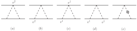
Figure 13: Diagrams with two-graviton exchange.

In Fig. 13 we show all diagrams with two-graviton exchange that enter at the second PN order. The sum of those diagrams is

$$L_{Fig13}=\sum_{a\neq b}\frac{G^{2}m_{a}^{2}m_{b}}{4r^{4}}\left(6r^{2}\mathbf{v}_{a}^{2}+7r^{2}\mathbf{v}_{b}^{2}-14r^{2}\mathbf{v}_{a}\cdot\mathbf{v}_{b}+2\dot{r}\mathbf{v}_{a}\cdot\mathbf{r}-2\mathbf{v}_{a}\cdot\mathbf{r}\mathbf{v}_{b}\cdot\mathbf{r}\right).$$ (145)

Figure 14: (a) three-graviton emission from one of the bodies; (b) symmetric three-graviton exchange; (c) composition of a three-graviton vertex with a two-graviton vertex in the source term.

There is also the diagram with a three-graviton source term as well as other two diagrams with combinations of the two-graviton source, as shown in Fig. 14. Their contribution to the Lagrangian is

$$L_{Fig14}=-\sum_{a\neq b}\frac{G^{3}m_{a}^{2}m_{b}}{2r^{3}}\left(m_{a}+3m_{b}\right).$$ (146)

Figure 15: Diagrams with three-graviton exchange.

The diagrams which contain three-graviton vertices are illustrated in Fig. 15 and give

$$L_{Fig15}=\sum_{a\neq b}\frac{G^{2}m_{a}^{2}m_{b}}{2r^{4}}\left[r^{2}\left(5\mathbf{v}_{a}^{2}-6\mathbf{v}_{a}\cdot\mathbf{v}_{b}+2\mathbf{v}_{b}^{2}+2\mathbf{a}_{b}\cdot\mathbf{r}\right)-9\left(\mathbf{v}_{a}\cdot\mathbf{r}\right)^{2}+14\mathbf{v}_{a}\cdot\mathbf{r}\mathbf{v}_{b}\cdot\mathbf{r}-3\left(\mathbf{v}_{b}\cdot\mathbf{r}\right)^{2}\right].$$ (147)

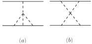
Figure 16: Diagrams with four-graviton vertex.

In Fig. 16, we show diagrams with a four-graviton vertex that enter at the 2PN order and, together, yield the result

$$L_{Fig16}=\sum_{a\neq b}\frac{G^{3}m_{a}^{3}m_{b}}{r^{3}}.$$ (148)

Figure 17: Diagrams with five propagators.

Lastly, the diagrams with five propagators are shown in Fig. 17 and provide us with the following result:

$$L_{Fig17}=\sum_{a\neq b}\frac{G^{3}m_{a}^{2}m_{b}}{r^{3}}\left(m_{b}-2m_{a}\right).$$ (149)

Summing up all contributions from Fig. 11 to Fig. 17, we write down the Lagrangian at 2PN order in the linearized harmonic gauge:

$$L_{2PN} =\frac{1}{16}m_{1}\mathbf{v}_{1}^{6}-\frac{G^{3}m_{1}m_{2}}{2r^{3}}\left(3m_{1}^{2}+m_{1}m_{2}\right)+\frac{G^{2}m_{1}m_{2}}{4r^{2}}\left[\left(16m_{1}+11m_{2}\right)\mathbf{v}_{1}^{2}\right.$$

$$\left.-13m\mathbf{v}_{1}\cdot\mathbf{v}_{2}-4m_{2}\mathbf{a}_{1}\cdot\mathbf{r}-\frac{2}{r^{2}}\left(8m_{1}+3m_{2}\right)\left(\mathbf{v}_{1}\cdot\mathbf{r}\right)^{2}+\frac{12}{r^{2}}m\mathbf{v}_{1}\cdot\mathbf{r}\mathbf{v}_{2}\cdot\mathbf{r}\right]$$

$$+\frac{Gm_{1}m_{2}}{8r}\left[\frac{15}{2}r^{2}\mathbf{a}_{1}\cdot\mathbf{a}_{2}+7\mathbf{v}_{1}^{4}-10\mathbf{v}_{1}^{2}\mathbf{v}_{1}\cdot\mathbf{v}_{2}+\left(\mathbf{v}_{1}\cdot\mathbf{v}_{2}\right)^{2}+\frac{3}{2}\mathbf{v}_{1}^{2}\mathbf{v}_{2}^{2}\right.$$

$$+\mathbf{a}_{1}\cdot\mathbf{r}\mathbf{v}_{2}^{2}-14\mathbf{a}_{1}\cdot\mathbf{v}_{2}\mathbf{v}_{2}\cdot\mathbf{r}+12\mathbf{a}_{1}\cdot\mathbf{v}_{1}\mathbf{v}_{2}\cdot\mathbf{r}-\frac{1}{2}\mathbf{a}_{1}\cdot\mathbf{r}\mathbf{a}_{2}\cdot\mathbf{r}-\frac{1}{r^{2}}\mathbf{a}_{1}\cdot\mathbf{r}\left(\mathbf{v}_{2}\cdot\mathbf{r}\right)^{2}$$

$$\left.+\frac{1}{r^{2}}\left(6\mathbf{v}_{1}\cdot\mathbf{r}\mathbf{v}_{2}\cdot\mathbf{r}\mathbf{v}_{1}\cdot\mathbf{v}_{2}-\left(\mathbf{v}_{1}\cdot\mathbf{r}\right)^{2}\mathbf{v}_{2}^{2}-6\mathbf{v}_{1}\cdot\mathbf{r}\mathbf{v}_{2}\cdot\mathbf{r}\mathbf{v}_{2}^{2}+\frac{3}{2r^{2}}\left(\mathbf{v}_{1}\cdot\mathbf{r}\right)^{2}\left(\mathbf{v}_{2}\cdot\mathbf{r}\right)^{2}\right)\right]$$

$$+1\leftrightarrow 2.$$ (150)

We use the Lagrangian above to determine the equations of motion of the two-body system at the second PN order. Below we show the acceleration for one of the objects in the binary:

$$\mathbf{a}_{1}^{2PN} =\frac{1}{8}\frac{Gm_{2}}{r^{3}}\mathbf{r}\left\{\frac{G^{2}}{r^{2}}\left(-2m_{1}^{2}-20m_{1}m_{2}+16m_{2}^{2}\right)+\frac{G}{r}\left[\left(18m_{1}+56m_{2}\right)\mathbf{v}_{1}^{2}\right.\right.$$

$$-\left(84m_{1}+128m_{2}\right)\mathbf{v}_{1}\cdot\mathbf{v}_{2}+\left(58m_{1}+64m_{2}\right)\mathbf{v}_{2}^{2}+30m_{1}\mathbf{a}_{1}\cdot\mathbf{r}-12m\mathbf{a}_{2}\cdot\mathbf{r}$$

$$\left.+\frac{28}{r^{2}}\left(m_{1}-4m_{2}\right)\mathbf{v}_{1}\cdot\mathbf{r}\left(\mathbf{v}_{1}\cdot\mathbf{r}-2\mathbf{v}_{2}\cdot\mathbf{r}\right)-\frac{1}{r^{2}}\left(56m_{1}+176m_{2}\right)\left(\mathbf{v}_{2}\cdot\mathbf{r}\right)^{2}\right]$$

$$+2\mathbf{v}_{1}^{4}-16\left(\mathbf{v}_{1}\cdot\mathbf{v}_{2}\right)^{2}-16\mathbf{v}_{2}^{4}+32\mathbf{v}_{1}\cdot\mathbf{v}_{2}\mathbf{v}_{2}^{2}-2\mathbf{v}_{1}^{2}\mathbf{a}_{2}\cdot\mathbf{r}-2\mathbf{v}_{2}^{2}\mathbf{a}_{2}\cdot\mathbf{r}$$

$$\left.-4\mathbf{a}_{2}\cdot\mathbf{v}_{2}\mathbf{v}_{2}\cdot\mathbf{r}+\frac{\left(\mathbf{v}_{2}\cdot\mathbf{r}\right)^{2}}{r^{2}}\left(12\mathbf{v}_{1}^{2}-48\mathbf{v}_{1}\cdot\mathbf{v}_{2}+36\mathbf{v}_{2}^{2}\right)-15\frac{\left(\mathbf{v}_{2}\cdot\mathbf{r}\right)^{4}}{r^{4}}\right\}$$

$$+\frac{1}{4}\frac{Gm_{2}}{r^{3}}\mathbf{v}_{1}\left\{\frac{G}{r}\left[\left(48m_{2}-15m_{1}\right)\mathbf{v}_{1}\cdot\mathbf{r}+\left(23m_{1}-40m_{2}\right)\mathbf{v}_{2}\cdot\mathbf{r}\right]\right.$$

$$+\mathbf{v}_{2}\cdot\mathbf{r}\left(4\mathbf{v}_{1}^{2}+16\mathbf{v}_{1}\cdot\mathbf{v}_{2}-20\mathbf{v}_{2}^{2}\right)-24\frac{\mathbf{v}_{1}\cdot\mathbf{r}\left(\mathbf{v}_{2}\cdot\mathbf{r}\right)^{2}}{r^{2}}+18\frac{\left(\mathbf{v}_{2}\cdot\mathbf{r}\right)^{3}}{r^{2}}$$

$$\left.+\mathbf{v}_{1}\cdot\mathbf{r}\left(8\mathbf{v}_{1}^{2}-16\mathbf{v}_{1}\cdot\mathbf{v}_{2}+16\mathbf{v}_{2}^{2}-2\mathbf{a}_{2}\cdot\mathbf{r}\right)+2r^{2}\left(12\mathbf{a}_{1}-7\mathbf{a}_{2}\right)\cdot\mathbf{v}_{1}\right\}$$

$$+2\mathbf{a}_{1}\cdot\mathbf{v}_{1}\mathbf{v}_{1}^{2}\mathbf{v}_{1}+\frac{1}{4}\mathbf{a}_{1}\left(49\frac{G^{2}m_{1}m_{2}}{r^{2}}+36\frac{G^{2}m_{2}^{2}}{r^{2}}+12\frac{Gm_{2}}{r}\mathbf{v}_{1}^{2}+\mathbf{v}_{1}^{4}\right)$$

$$+\frac{1}{4}\frac{Gm_{2}}{r^{3}}\mathbf{v}_{2}\left\{\frac{G}{r}\left[\left(31m_{1}-24m_{2}\right)\mathbf{v}_{1}\cdot\mathbf{r}+\left(40m_{2}-9m_{1}\right)\mathbf{v}_{2}\cdot\mathbf{r}\right]\right.$$

$$+\mathbf{v}_{2}\cdot\mathbf{r}\left(-4\mathbf{v}_{1}^{2}-16\mathbf{v}_{1}\cdot\mathbf{v}_{2}+20\mathbf{v}_{2}^{2}\right)+24\frac{\mathbf{v}_{1}\cdot\mathbf{r}\left(\mathbf{v}_{2}\cdot\mathbf{r}\right)^{2}}{r^{2}}-18\frac{\left(\mathbf{v}_{2}\cdot\mathbf{r}\right)^{3}}{r^{2}}$$

$$\left.+\mathbf{v}_{1}\cdot\mathbf{r}\left(16\mathbf{v}_{1}\cdot\mathbf{v}_{2}-16\mathbf{v}_{2}^{2}\right)-14r^{2}\mathbf{a}_{2}\cdot\mathbf{v}_{2}\right\}$$

$$-\frac{7}{4}\frac{Gm_{2}}{r}\mathbf{a}_{2}\left(6\frac{Gm}{r}+\mathbf{v}_{1}^{2}+\mathbf{v}_{2}^{2}\right).$$ (151)

All accelerations in the right hand side of the equality above should be regarded as Newtonian accelerations if we want the entire expression to be of definite 2PN order. To write the acceleration in the center of mass frame, we have to consider, in addition to (151), the reduced contribution from applying the equation of motion inside the (72) as well as the PN corrections to the center of mass frame (93) and (94). Adding these contributions together, we finally obtain the expression for the relative acceleration of the two-body system in the center of mass frame, at the second PN order, in the linearized harmonic gauge:

$$\mathbf{a}_{2PN} =-\frac{Gm}{8r^{3}}\left\{\mathbf{r}\left[\left(56+174\nu\right)\frac{G^{2}m^{2}}{r^{2}}-\left(32+52\nu-16\nu^{2}\right)\frac{Gm}{r}v^{2}+\left(112-200\nu-16\nu^{2}\right)\frac{Gm}{r}\dot{r}^{2}\right.\right.$$

$$\left.+\left(24\nu-32\nu^{2}\right)v^{4}-\left(36\nu-48\nu^{2}\right)v^{2}\dot{r}^{2}+\left(15\nu-45\nu^{2}\right)\dot{r}^{4}\right]$$

$$\left.+4r\dot{r}\mathbf{v}\left[\left(-12+41\nu+8\nu^{2}\right)\frac{Gm}{r}-\left(15\nu+4\nu^{2}\right)v^{2}+\left(9\nu+6\nu^{2}\right)\dot{r}^{2}\right]\right\}.$$ (152)

References

[1]
B. P. Abbott et al.
Observation of Gravitational Waves from a Binary Black Hole Merger.
Phys. Rev. Lett., 116(6):061102, 2016.
[2]
B. P. Abbott et al.
Astrophysical Implications of the Binary Black-Hole Merger
GW150914.
Astrophys. J., 818(2):L22, 2016.
[3]
B. P. Abbott et al.
Binary Black Hole Mergers in the first Advanced LIGO Observing Run.
Phys. Rev., X6(4):041015, 2016.
[4]
B. P. Abbott et al.
Gw170104: Observation of a 50-solar-mass binary black hole
coalescence at redshift 0.2.
Phys. Rev. Lett., 118:221101, Jun 2017.
[5]
B. P. Abbott et al.
Gw170814: A three-detector observation of gravitational waves from a
binary black hole coalescence.
Phys. Rev. Lett., 119:141101, Oct 2017.
[6]
B. P. Abbott et al.
Gw170817: Observation of gravitational waves from a binary neutron
star inspiral.
Phys. Rev. Lett., 119:161101, Oct 2017.
[7]
B. P. Abbott et al.
GW170608: Observation of a 19 solar-mass binary black hole
coalescence.
The Astrophysical Journal, 851(2):L35, dec 2017.
[8]
B. P. Abbott et al.
Gwtc-1: A gravitational-wave transient catalog of compact binary
mergers observed by ligo and virgo during the first and second observing
runs.
Phys. Rev. X, 9:031040, Sep 2019.
[9]
B. P. Abbott et al.
Gravitational waves and gamma-rays from a binary neutron star merger:
GW170817 and GRB 170817a.
The Astrophysical Journal, 848(2):L13, oct 2017.
[10]
B. P. Abbott et al.
Multi-messenger observations of a binary neutron star merger.
The Astrophysical Journal, 848(2):L12, oct 2017.
[11]
B. P. Abbott et al.
Low-latency gravitational-wave alerts for multimessenger astronomy
during the second advanced LIGO and virgo observing run.
The Astrophysical Journal, 875(2):161, apr 2019.
[12]
Walter D. Goldberger and Ira Z. Rothstein.
An Effective field theory of gravity for extended objects.
Phys.Rev., D73:104029, 2006.
[13]
Walter D. Goldberger.
Les Houches lectures on effective field theories and gravitational
radiation.
In Les Houches Summer School - Session 86: Particle Physics and
Cosmology: The Fabric of Spacetime Les Houches, France., 2007.
[14]
Ira Z. Rothstein.
Progress in effective field theory approach to the binary inspiral
problem.
Gen. Rel. Grav., 46:1726, 2014.
[15]
Stefano Foffa and Riccardo Sturani.
Effective field theory methods to model compact binaries.
Class. Quant. Grav., 31(4):043001, 2014.
[16]
Rafael A. Porto.
The effective field theorist’s approach to gravitational
dynamics.
Phys. Rept., 633:1–104, 2016.
[17]
Michele Levi.
Effective Field Theories of Post-Newtonian Gravity: A comprehensive
review.
2018.
[18]
Stefano Foffa and Riccardo Sturani.
Conservative dynamics of binary systems to fourth Post-Newtonian
order in the EFT approach I: Regularized Lagrangian.
Phys. Rev., D100(2):024047, 2019.
[19]
Stefano Foffa, Rafael A. Porto, Ira Rothstein, and Riccardo Sturani.
Conservative dynamics of binary systems to fourth Post-Newtonian
order in the EFT approach II: Renormalized Lagrangian.
Phys. Rev., D100(2):024048, 2019.
[20]
Donato Bini and Thibault Damour.
Analytical determination of the two-body gravitational interaction
potential at the fourth post-Newtonian approximation.
Phys. Rev., D87(12):121501, 2013.
[21]
Thibault Damour, Piotr Jaranowski, and Gerhard Schafer.
Nonlocal-in-time action for the fourth post-Newtonian conservative
dynamics of two-body systems.
Phys. Rev., D89(6):064058, 2014.
[22]
Laura Bernard, Luc Blanchet, Alejandro Bohe, Guillaume Faye, and Sylvain
Marsat.
Fokker action of nonspinning compact binaries at the fourth
post-Newtonian approximation.
Phys. Rev., D93(8):084037, 2016.
[23]
Laura Bernard, Luc Blanchet, Alejandro Bohe, Guillaume Faye, and Sylvain
Marsat.
Energy and periastron advance of compact binaries on circular orbits
at the fourth post-Newtonian order.
Phys. Rev., D95(4):044026, 2017.
[24]
Rafael A. Porto, Andreas Ross, and Ira Z. Rothstein.
Spin induced multipole moments for the gravitational wave flux from
binary inspirals to third Post-Newtonian order.
JCAP, 1103:009, 2011.
[25]
Rafael A. Porto, Andreas Ross, and Ira Z. Rothstein.
Spin induced multipole moments for the gravitational wave amplitude
from binary inspirals to 2.5 Post-Newtonian order.
JCAP, 1209:028, 2012.
[26]
Walter D. Goldberger and Andreas Ross.
Gravitational radiative corrections from effective field theory.
Phys. Rev., D81:124015, 2010.
[27]
Luc Blanchet, Guillaume Faye, Bala R. Iyer, and Benoit Joguet.
Gravitational wave inspiral of compact binary systems to 7/2
postNewtonian order.
Phys. Rev., D65:061501, 2002.
[Erratum: Phys. Rev.D71,129902(2005)].
[28]
Andreas Ross.
Multipole expansion at the level of the action.
Phys. Rev., D85:125033, 2012.
[29]
James B. Gilmore and Andreas Ross.
Effective field theory calculation of second post-Newtonian binary
dynamics.
Phys. Rev., D78:124021, 2008.
[30]
Barak Kol and Michael Smolkin.
Non-relativistic gravitation: from newton to einstein and back.
Classical and Quantum Gravity, 25(14):145011, jun 2008.
[31]
Rafael A. Porto and Ira Z. Rothstein.
Apparent ambiguities in the post-Newtonian expansion for binary
systems.
Phys. Rev., D96(2):024062, 2017.
[32]
Benjamin Grinstein and Ira Z. Rothstein.
Effective field theory and matching in nonrelativistic gauge
theories.
Phys. Rev., D57:78–82, 1998.
[33]
Clifford Cheung, Ira Z. Rothstein, and Mikhail P. Solon.
From Scattering Amplitudes to Classical Potentials in the
Post-Minkowskian Expansion.
Phys. Rev. Lett., 121(25):251101, 2018.
[34]
Chad R. Galley and Adam K. Leibovich.
Radiation reaction at 3.5 post-newtonian order in effective field
theory.
Phys. Rev. D, 86:044029, Aug 2012.
[35]
Luc Blanchet.
Gravitational Radiation from Post-Newtonian Sources and Inspiralling
Compact Binaries.
Living Rev.Rel., 17(1):2, 2014.
[36]
A. Einstein, L. Infeld, and B. Hoffman.
Progress in effective field theory approach to the binary inspiral
problem.
Annals Math., 39:65, 1938.
[37]
Laura Bernard, Luc Blanchet, Guillaume Faye, and Tanguy Marchand.
Center-of-mass equations of motion and conserved integrals of compact
binary systems at the fourth post-newtonian order.
Phys. Rev. D, 97:044037, Feb 2018.
[38]
Lawrence E. Kidder.
Coalescing binary systems of compact objects to postNewtonian 5/2
order. 5. Spin effects.
Phys. Rev., D52:821–847, 1995.
[39]
Clifford M. Will and Alan G. Wiseman.
Gravitational radiation from compact binary systems: Gravitational
waveforms and energy loss to second post-newtonian order.
Phys. Rev. D, 54:4813–4848, Oct 1996.
[40]
A. Gopakumar and Bala R. Iyer.
Gravitational waves from inspiraling compact binaries: Angular
momentum flux, evolution of the orbital elements, and the waveform to the
second post-newtonian order.
Phys. Rev. D, 56:7708–7731, Dec 1997.
[41]
J. M. Martin-Garcia.
xAct: Efficient tensor computer algebra for the Wolfram Language.
https://www.xAct.es.
[42]
Michael E. Peskin and Daniel V. Schroeder.
An Introduction to quantum field theory.
Addison-Wesley, Reading, USA, 1995.