Quantum phase transitions on the hexagonal lattice

Abstract

Hubbard-type models on the hexagonal lattice are of great interest, as they provide realistic descriptions of graphene and other related materials. Hybrid Monte Carlo simulations offer a first-principles approach to study their phase structure. Here, we review the present status of our work in this direction.

1 Introduction

The Hubbard model, which describes fermionic quasi particles with contact interactions, continues to be of profound interest, as it remains the quintessential example of an interacting fermion system, and can qualitatively describe many non-perturbative phenomena, such as dynamical mass-gap generation or superconductivity. On the honeycomb lattice, extended versions with varying on-site, nearest- and next-to-nearest-neighbor interactions have been predicted to host a large variety of gapped phases, such as spin-density wave (SDW) and charge-density wave (CDW) phases, topological insulators and spontaneous Kekulé distortions, many of which can be realized using ultra-cold atoms trapped in optical lattices [1, 2] or other experimental techniques. Long-range interaction potentials realistically describe the physics of both mono- and bilayer graphene [3, 4]. Determinantal Quantum Monte Carlo simulations following Blankenbecler, Scalapino and Sugar (BSS) remain the method of choice for obtaining first-principles results for fermionic systems with contact interactions. In recent years however, the Hybrid-Monte-Carlo (HMC) method, which has a long history in high-energy physics, has found increasing application for the study of Hubbard-type models with off-site interactions, as it can efficiently simulate non-diagonal interaction matrices.

In this article, we review a number of different results which we obtained by applying HMC on the honeycomb lattice. After presenting the basics of the numerical setup (section 2), we start with a discussion of the extended Hubbard model with on-site ($U$) and nearest-neighbor ($V_{1}$) interactions (section 3). In this model, we studied the competition between SDW and CDW order and determined the location and critical properties of a phase boundary separating a semimetal from a SDW phase [5]. Next we turn to the realistic long-range potential of graphene (section 4), which exhibits a semimetal-SDW transition in the strong-coupling regime. By studying its critical properties we found an inconsistency with the Gross-Neveu universality class, which applies in the case of short-range interactions, and concluded that a conformal phase transition provides a more natural explanation for our results [6]. Third we discuss graphene at finite spin density (section 5). We focus here on the topological neck-disrupting Lifshitz transition, which occurs when the Fermi level traverses saddle points in the single-particle bands, and which is accompanied by a logarithmic divergence of the density of states and correspondingly the ferromagnetic susceptibility. We found that this divergence follows a powerlaw in the presence of interactions and is driven by the disconnected rather than the connected susceptibility, indicating an instability towards formation of ordered electronic phases [7]. And finally we discuss graphene with hydrogen adatoms, which can be modeled as vacant lattice sites (section 6). Here we showed that the pairwise Ruderman-Kittel-Kasuya-Yosida (RKKY) potential between adatoms is strongly affected by inter-electron interactions, such that dimer formation is suppressed, and that certain configurations of adatom superlattices are dynamically stabilized [8]. We end with a short outlook (section 7).

2 Numerical setup

The starting point is the interacting tight-binding theory on the honeycomb lattice. In the most general form which we consider, the Hamiltonian is given by:

$$\hat{\mathcal{H}}=-\kappa\sum_{\left\langle x,y\right\rangle,\sigma}\left(\hat{c}^{\dagger}_{x,\sigma}\hat{c}_{y,\sigma}+\textrm{h.c.}\right)+\frac{1}{2}\sum_{x,y}\hat{q}_{x}V_{xy}\hat{q}_{y}+\sum_{x}m_{s}\left(\hat{c}^{\dagger}_{x,\uparrow}\hat{c}_{x,\uparrow}-\hat{c}^{\dagger}_{x,\downarrow}\hat{c}_{x,\downarrow}\right).$$ (1)

Here $\kappa$ is the hopping energy, $\langle x,y\rangle$ denotes nearest-neighbor sites, $\sigma=\uparrow,\downarrow$ labels spin directions, $\hat{q}_{x}=\hat{c}^{\dagger}_{x,\uparrow}\hat{c}_{x,\uparrow}+\hat{c}^{\dagger}_{x,\downarrow}\hat{c}_{x,\downarrow}-1$ is the electric charge operator and $m_{s}$ denotes a “staggered” mass, which has an opposite sign on the two triangular sublattices and is added to remove zero modes (we will specify below when we used a non-zero $m_{s}$). The creation- and annihilation operators satisfy the anticommutation relations $\{\hat{c}_{x,\sigma},\hat{c}^{\dagger}_{y,\sigma^{\prime}}\}=\delta_{x,y}\delta_{\sigma,\sigma^{\prime}}$. The matrix elements $V_{xy}$ can be chosen freely to describe different two-body potentials and are only restricted by the condition that $V$ be positive definite (different choices are used in each of the projects discussed below). The theoretical groundwork for HMC simulations of (1) was originally worked out in [9]. We will present a compact summary here, which also takes some more recent developments into account.

HMC is based on the path-integral formulation of the (grand-canonical) partition function ${\cal Z}$. To derive it, we start with a symmetric Suzuki-Trotter decomposition, which yields

$${\cal Z}=\Tr\left(e^{-\beta\hat{\mathcal{H}}}\right)=\Tr\left(e^{-\delta_{\tau}\hat{\mathcal{H}}_{0}}e^{-\delta_{\tau}\hat{\mathcal{H}}_{\mathrm{int}}}e^{-\delta_{\tau}\hat{\mathcal{H}}_{0}}\dots\right)+O(\delta^{2}_{\tau})~{}.$$ (2)

Here we have separated the interacting and non-interacting contributions to (1) and introduced a finite stepsize $\delta_{\tau}=\beta/N_{t}$ in Euclidean time. We now apply two variable transformations. The first is a canonical transformation where creation- and annihilation operators for spin-down particles are replaced by hole operators, and the sign of these is flipped on one sublattice, i.e. a transformation of the form

$$\hat{c}_{x,\uparrow},\hat{c}^{\dagger}_{x,\uparrow}\to\hat{a}_{x},\hat{a}^{\dagger}_{x},\quad\quad\quad\hat{c}_{x,\downarrow},\hat{c}^{\dagger}_{x,\downarrow}\to\pm\hat{b}^{\dagger}_{x},\pm\hat{b}_{x}~{}.$$ (3)

This step is necessary to avoid a fermion sign problem (i.e. an indefinite measure of the path integral), and can only be applied on bipartite lattices. The second is a Fierz transformation, which is applied to the on-site interaction term and which mixes charge and spin sectors. It has the form

$$\frac{V_{xx}}{2}\hat{q}_{x}^{2}=\eta\frac{V_{xx}}{2}\hat{q}_{x}^{2}-(1-\eta)\frac{V_{xx}}{2}(\hat{q}_{x}^{\prime})^{2}+V_{xx}(1-\eta)\,\hat{q}_{x}^{\prime},$$ (4)

where $\hat{q}_{x}^{\prime}=\hat{a}^{\dagger}_{x}\hat{a}_{x}+\hat{b}^{\dagger}_{x}\hat{b}_{x}$ is the spin-density operator and the constant $\eta$ can be chosen in the range $(0,1)$. As we will see below, this leads to the complexification of the auxiliary fields which we introduce, and serves to maintain ergodicity of HMC trajectories in absence of a staggered mass $m_{s}$.

Expressing ${\cal Z}$ as an integral over classical field variables, which can then be sampled stochastically, requires removing the fermionic operators from (2). This can be done by a form of Gaussian integration if the exponentials contain only bilinears. The fourth-power terms which appear in $\hat{\mathcal{H}}_{\mathrm{int}}$ must thus be removed, which is done by a Hubbard-Stratonovich transformation. We apply two different variants to interaction terms coupling to $\hat{q}_{x}$ and $\hat{q}_{x}^{\prime}$. The first term $\sim\eta\hat{q}_{x}^{2}$ appearing on the right hand side of (4) is re-absored into the interaction matrix $V_{xy}$ and the combined expression is then transformed using

$$\exp\left(-\frac{\delta_{\tau}}{2}\sum_{x,y}\hat{q}_{x}V_{xy}\hat{q}_{y}\right)\cong\int D\phi\,\exp\left(-\frac{1}{2\delta_{\tau}}\sum_{x,y}\phi_{x}V^{-1}_{xy}\phi_{y}+i\delta_{\tau}\sum_{x}\phi_{x}\,\hat{q}_{x}\right).$$ (5)

The $\sim(1-\eta)(\hat{q}_{x}^{\prime})^{2}$ term is transformed by its own, using

$$\exp\left(\frac{\delta_{\tau}}{2}(1-\eta)\sum_{x}V_{xx}(\hat{q}_{x}^{\prime})^{2}\right)\cong\int D\chi\,\exp\left(-\frac{1}{2\delta_{\tau}}\sum_{x}\frac{\chi^{2}_{x}}{(1-\eta)V_{xx}}+\delta_{\tau}\sum_{x}\chi_{x}\,\hat{q}_{x}^{\prime}\right).$$ (6)

In effect, we have introduced a complex auxiliary field variable (with real part $\chi$ and imaginary part $i\phi$) at each site of the $2+1$ dimensional hypercubic lattice. The third term in (4) is absorbed into $\chi$ by the transformation $\chi\to\chi-\delta_{\tau}V_{xx}(1-\eta)$.

To compute the trace in the fermionic Fock space (with anti-periodic boundary conditions) appearing in (2) we use

$$\Tr\left(e^{-\hat{A}_{1}}e^{-\hat{A}_{2}}\ldots e^{-\hat{A}_{n}}\right)={\rm det}\left(\begin{array}[]{cccc}1&-e^{-A_{1}}&0&\ldots\\ 0&1&-e^{-A_{2}}&\ldots\\ \vdots&&\ddots&\\ e^{-A_{n}}&0&\ldots&1\\ \end{array}\right),$$ (11)

where $\hat{A}_{k}=\left(A_{k}\right)_{ij}\hat{c}^{{\dagger}}_{i}\hat{c}_{j}$ are the fermionic bilinear operators and $A_{k}$ (without hat) contain matrix elements in the single-particle Hilbert space (this identity is derived in  [10, 11]). We finally obtain

$${\cal Z}=\int D\Phi\,|\textrm{det}[M(\Phi)]|^{2}e^{-S_{\eta}(\Phi)},\,$$ (12)

with

$$S_{\eta}(\Phi)=\frac{1}{2\delta_{\tau}}\sum_{x,y,t}\phi_{x,t}\widetilde{V}_{xy}^{-1}\phi_{y,t}+\sum_{x,t}\frac{(\chi_{x,t}-(1-\eta)\delta_{\tau}V_{xx})^{2}}{2(1-\eta)\delta_{\tau}V_{xx}}.$$ (13)

Here $\widetilde{V}$ denotes a modified interaction matrix wherein the diagonal elements have been rescaled by a factor of $\eta$ by (4). $|\textrm{det}[M(\Phi)]|^{2}$ appears in (12) since, after the particle-hole transformation (3), the spin-up and spin-down electrons contribute as $M$ and $M^{\dagger}$ respectively.

Two versions of the fermion matrix $M(\Phi)$ are used in this work which agree up to discretization effects. The first a full exponential form which follows directly from (11) and which respects the full spin- and sublattice symmetries of the continuum limit but is non-sparse and must be inverted by a special Schur complement solver (see [5] for a discussion). The second is obtained by a linearization of terms $e^{-\delta_{\tau}h}$ where $h$ denotes the single-particle tight-binding hopping matrix. This form respects the above mentioned symmetries only in the time-continuum limit, but is sparse and thus can be inverted by a standard conjugate gradient solver (see e.g. [12] and [7]). As the expressions for the fermion matrices are rather lengthy and differ between the works summarized in this review, we refer the interested reader to the original publications. For a discussion of the relative advantages of different fermion discretizations, see [13] and [14].

The HMC algorithm essentially consists of combining the classical time evolution of $\Phi$ in computer time with a stochastic refreshment of an associated momentum field $\pi$. A stochastic representation of the fermion determinants

$$|{\rm det}\left(M\right)(\Phi)|^{2}=\int D\Psi\Psi^{\dagger}e^{-\Psi^{\dagger}(MM^{\dagger})^{-1}\Psi},$$ (14)

is used, which introduces an additional pseudofermionic field $\Psi$ (this is a regular complex-valued field, not a set of Grassmann variables). Ultimately, we must numerically solve the Hamiltonian system given by

$${\cal H}=S_{\eta}(\Phi)+\Psi^{\dagger}(MM^{\dagger})^{-1}\Psi+\frac{\pi^{T}\pi}{2}~{},\quad\left[\frac{d\Phi}{d\tau}\right]^{T}=\frac{\partial{\cal H}}{\partial\pi}~{},\quad\left[\frac{d\pi}{d\tau}\right]^{T}=-\frac{\partial{\cal H}}{\partial\Phi}~{}.$$ (15)

A symplectic integrator is employed, which introduces a stepsize error, which is then corrected by a Metropolis accept/reject step. The full algorithm reads as follows:

• Refresh momentum field $\pi$ using Gaussian noise: $P(\pi)\sim e^{-\pi^{2}/2}$ .

• Refresh pseudofermions $\Psi$ by generating field $\rho$ with $P(\rho)=e^{-\rho^{\dagger}\rho}$ and obtaining $\Psi=M\rho$ .

• Do Hamiltonian evolution of $\pi$ and $\Phi$ by solving (15) with symplectic integrator (“molecular dynamics trajectory”).

• Accept new configuration with probability $P=\min(1,e^{-\Delta{\cal H}})$ (“Metropolis check”).

• Continue from step 1).

Additional details can be found in [12] and [5].

We point out here that a variant of HMC which avoids the use of pseudofermions was described and used in [6]. We also point out that we have omitted a discussion of boundary conditions. We used periodic boundary conditions in space in each project discussed here, either of the Born-von Kármán type or with a rectangular geometry. The exact type can be found in the original literature.

3 Competing order in the extended Hubbard model

The hexagonal Hubbard model with pure on-site interaction has been studied fairly extensively with Quantum Monte Carlo methods [15, 16, 17]. By now it is well established that it exhibits a second order phase transition from a semimetal to a gapped SDW phase if the onsite potential is increased above $U\approx 3.8\kappa$. The universality class of the $2+1D$ chiral Gross-Neveu model has been verified for this transition and several critical exponents have been obtained with fairly high precision. However, energy balance arguments and renormalization group calculations suggest that a CDW phase might be favored in some region of the phase diagram if a nearest-neighbor potential $V_{1}$ is included (see e.g. [18]). To detect a particular phase one may use external sources. For instance, the staggered mass $m_{s}$ introduced in (1) couples to an anti-ferromagnetic condensate, and by extrapolating it to the $m_{s}\to 0$ and thermodynamic limits one may probe the semimetal-SDW transition. To study competing phases one must add multiple sources, so extrapolations in a high-dimensional parameter space are required. More importantly however, a corresponding source term for CDW order introduces a sign problem and cannot be simulated, even in principle.

In [5] we carried out an unbiased study of the competition between CDW and SDW order in the $U-V_{1}$ plane by avoiding the use source terms altogether. We used observables of the form

$$\langle X^{2}\rangle=\left\langle\frac{1}{L^{4}}\left(\sum\limits_{x\in A}\hat{X}_{x}\right)^{2}\right\rangle+\left\langle\frac{1}{L^{4}}\left(\sum\limits_{x\in B}\hat{X}_{x}\right)^{2}\right\rangle,$$ (16)

where the sums run over the two triangular sublattices (“A” and “B”) respectively and $L$ is the linear lattice size. Observables of this type develop a non-zero expectation value even without explicit symmetry breaking. We considered two different observables, where $X$ is either the charge $q$ or a spin component $S_{i}$, with

$$\hat{S}_{x,i}=\frac{1}{2}(\hat{c}^{\dagger}_{x,\uparrow},\,\hat{c}^{\dagger}_{x,\downarrow})\sigma_{i}\left(\begin{array}[]{c}\hat{c}_{x,\uparrow}\\ \hat{c}_{x,\downarrow}\\ \end{array}\right).$$ (19)

Different spin components can be averaged over to improve statistics. We used the exponential fermion operator in this project, so the rotational symmetry of $\hat{S}$ is respected.

We point out here that the Hamiltonian possesses zero modes in absence of any mass terms, which partition the configuration space of a purely real or imaginary Hubbard field into disconnected sectors, separated by infinite potential barriers. It is for this principle reason that complex auxiliary fields were introduced in section 2. By choosing a mixing parameter $\eta$ which is only slightly smaller than one, HMC trajectories are able to circumvent these barriers, and ergodicity is recovered.

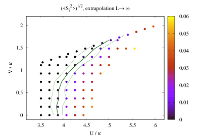
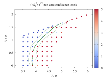
Figure 1: Figures taken from [5]. Left: Infinite volume extrapolation of $\sqrt{\langle S^{2}\rangle}$ using linear model $a+b\cdot(1/L)$. Right: Number of standard deviations with which non-zero $\sqrt{\langle S^{2}\rangle}$ is established in $L\to\infty$ limit. Both figures: Green lines mark the phase boundary with errorband, obtained from a finite size scaling study of $\langle S^{2}\rangle$.

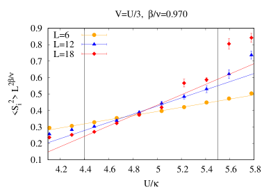
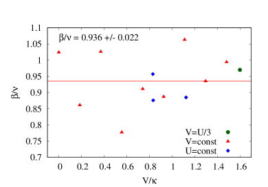
Figure 2: Figures taken from [5]. Left: Finite size scaling of $\langle S^{2}\rangle$ for $V_{1}=U/3$ (example). $\beta/\nu$ is chosen such that the enclosed triangle between fits to $L=6,12,18$ is minimized. Right: Optimal exponents $\beta/\nu$ for horizontal, vertical and diagonal lines in the phase diagram.

The requirement of a positive definite interaction matrix leads to the restriction $V_{1}<U/3$. To obtain the phase diagram in this region, we used a two step process. First we carried out infinite-volume extrapolations of $\sqrt{\langle S^{2}\rangle}$ and $\sqrt{\langle q^{2}\rangle}$. Both of these quantities turned out to have an approximately linear dependence on $1/L$, so the intercept of fits of the form $a+b\cdot(1/L)$ could be used to estimate the extent of ordered phases. This revealed that the SDW phase at large $U$ extends all the way to the $V_{1}=U/3$ line, while no evidence for CDW order was found. To supplement this result, a finite size scaling analysis of $\langle S^{2}\rangle$ was carried out close to the presumed phase boundary, along horizontal, vertical and diagonal lines. This revealed that the second order phase transition of the pure on-site model extends to $V_{1}=U/3$, and is likely described by the same critical exponents $\beta/\nu\approx 0.9$, consistent with Gross-Neveu universality. The results are summarized in figures 1 and 2, which are taken from [5].

4 Gap formation in graphene

While it is now firmly established that graphene in vacuum is a conductor, the question of the closest gapped phase in its phase diagram remains of interest, in particular in light of the rapid development of experimental techniques to control the microscopic interaction parameters and the emergence of other hexagonal materials. A crucial question thereby is the role of the Coulomb tail of the two-body potential, which is essentially unscreened in $2D$ materials. Strong-coupling expansions and renormalization group studies have suggested that dynamical gap formation is driven primarily by short-range interactions, which would imply a semimetal-SDW transition with Gross-Neveu universality for sufficiently strong coupling [19, 20]. In contrast, a Dyson-Schwinger study of the low-energy effective field theory of graphene, which is sensitive only to the long-range physics, predicted a (pseudo) conformal phase transition (CPT) governed by exponential (“Miransky”) scaling [21]. In principle the long-range part of the potential might also favor other phases, with CDW being the most likely candidate.

In the past we studied gap formation in graphene intensively using HMC [22, 23, 12]. These early works were focused on the detection of SDW order however, and employed source terms which explicitly favor such a phase. Moreover, the critical properties were never addressed. More recently, we thus decided to revisit this topic in a fully unbiased study without explicit sources [6], which also makes use of all of the most recent algorithmic developments, in particular the complexification of the Hubbard field and the exponential action. We review the results of this study here. For $V_{xy}$ we used a realistic two-body potential for graphene, which contains the exact interaction parameters obtained at short distances within a constrained random-phase approximation (cRPA) in [3], and is smoothly interpolated to an unscreened Coulomb tail using a thin-film model (see figure 3, left). To drive the system towards the semimetal-insulator phase transition, we rescaled this potential by a factor $\lambda>1$, so that suspended graphene corresponds to $\lambda=1$.

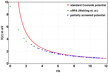
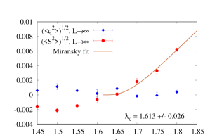
Figure 3: Figures taken from [6]. Left: Partially screened Coulomb potential compared with unscreened Coulomb potential (red). Points correspond to cRPA values (green) and thin-film model (blue) from [3]. Right: $L\to\infty$ limit of $\sqrt{\langle S^{2}\rangle}$ (red) and $\sqrt{\langle q^{2}\rangle}$ (blue). For spin a fit of (20) to points at $\lambda>1.61$ is shown.

We considered the same observables as in section 3, i.e. the squared spin $\langle S^{2}\rangle$ and squared charge $\langle q^{2}\rangle$ per sublattice as defined by (16), or their square roots respectively. Using linear fits of the form $f(1/L)=a+b\cdot(1/L)$ to lattice sizes $L=12,18,24$ we carried out an $L\to\infty$ extrapolation of $\sqrt{\langle S^{2}\rangle}$ and $\sqrt{\langle q^{2}\rangle}$ for a range of $\lambda$ values (see figure 3, right panel). We can immediately conclude that SDW order is favored over CDW order: while the extrapolation of $\sqrt{\langle q^{2}\rangle}$ is consistent with zero for any of the coupling strengths considered, $\sqrt{\langle S^{2}\rangle}$ develops a non-zero expectation value around $\lambda_{c}\approx 1.65$. By fitting the Miransky scaling function

$$\sigma(\lambda)=a\exp\left(\frac{-b}{\sqrt{\lambda-\lambda_{c}}}\right),$$ (20)

as appropriate for reduced QED₄ (see [21]) to $\sqrt{\langle S^{2}\rangle}|_{L=\infty}$, we can estimate $\lambda_{c}=1.61\pm 0.02$. Note that the quality of this fit does not necessarily imply the validity of the CPT scenario. A power-law fit works equally well, which reflects the difficulty of detecting Miransky scaling with direct methods.

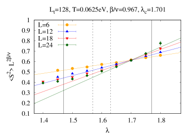
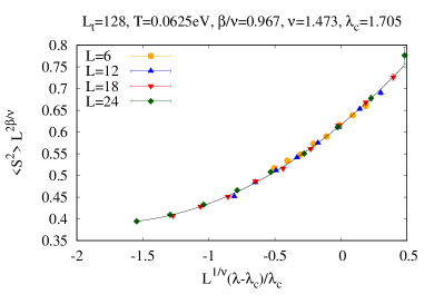
Figure 4: Figures taken from [6]. Left: Finite size scaling of $\langle S^{2}\rangle$ for graphene. $\beta/\nu$ chosen to minimize enclosed triangles between linear fits to $L=6,12,18,24$. Solid lines mark boundaries for all fits. Dashed lines mark lower bounds for $L=18,24$. Right: Collapse of $\langle S^{2}\rangle L^{2\beta/\nu}$ onto universal scaling function. $\beta/\nu$ taken from left panel. $\nu$ and $\lambda_{c}$ were optimized by minimizing the $\chi^{2}/\textrm{d.o.f.}$ of fits of all data to polynomial functions of $x=L^{1/\nu}(\lambda-\lambda_{c})/\lambda_{c}$.

To determine the critical properties, we first carried out a finite-size scaling study of $\langle S^{2}\rangle$. This was done by applying linear fits to $\langle S^{2}\rangle L^{2\beta/\nu}$ as a function of $\lambda$, and determining $\beta/\nu$ by minimizing the enclosed triangles between fits to $L=6,12,18,24$. While this procedure leads to $\beta/\nu\approx 0.97$ (slightly larger than the estimates for Gross-Neveu universality) for a particular choice of fit windows (see left panel of figure 4), we find that $\beta/\nu$ is not constrained very strongly by our data: by choosing different fit windows it is possible to obtain values in the range $0.95\ldots 1.0$, with corresponding estimates for $\lambda_{c}$ in the range $1.6\ldots 1.7$. We stress that this is rather unusual for a second order phase transition. In fact, we applied the same procedure to a set of test data obtained with onsite interactions $U$ only, and found that both $\beta/\nu$ and $U_{c}$ are tightly constrained in that case.

We also attempted to collapse all data-points onto a univeral scaling function, by plotting $\langle S^{2}\rangle L^{2\beta/\nu}$ over $x=L^{1/\nu}(\lambda-\lambda_{c})/\lambda_{c}$ and choosing $\nu$ such that the $\chi^{2}/\textrm{d.o.f.}$ of a fit of all data to a polynomial function $f(x)$ is minimized. This reveals a similarly puzzling situation. First, we find that the optimal exponent $\nu\approx 1.47$ is again much larger than for the Gross-Neveu model (which is $\nu\approx 1.2$). Perhaps more importantly however, we find that the constraints placed on $\nu$ again are very weak, with the quality of fit being not very sensitive to increases of $\nu$. This effect becomes even more pronounced when smaller lattice sizes are ignored. If we exclude all but the $L=18,24$ data from the fit we find that it is possible to increase $\nu$ almost indefinitely. This is very different from the pure Hubbard model, where we made an unsuccessful attempt to reproduce this feature. See figure 5 for an illustration.

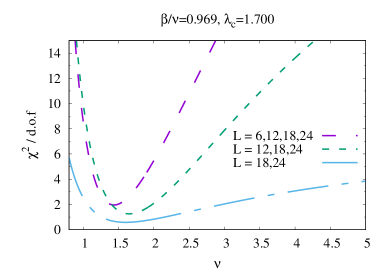
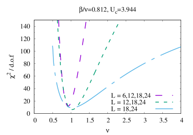
Figure 5: $\chi^{2}/\textrm{d.o.f}$ for collapse of $\langle S^{2}\rangle L^{2\beta/\nu}$ onto a universal finite-size scaling function for graphene (left) and Hubbard model (right) with different choices of $\nu$ for different sets of lattice sizes. $\beta/\nu$ and critical coupling strength are fixed to their optimal values. For graphene the quality of fit is rather insensitive to increases of $\nu$ when smaller lattices are excluded. Figures taken from [6].

We propose that the CPT offers a natural explanation for our results. In [21] it was argued that the CPT formally corresponds to the limit $\beta,\nu\to\infty$, $\delta=1$ of a second order transition and that the usual hyperscaling relations may apply. In our case $d=2$ (where $d$ is the number of spatial dimensions) and with $\delta=1$ the relation

$$\frac{\beta}{\nu}=\frac{d}{\delta+1}$$ (21)

would thus lead to $\beta/\nu=1$, which agrees with our estimate at a level of about $3\%$ and is well within the present errors. A CPT is also expected to receive power-law corrections and mimic a second order transition in finite volume. It is thus reasonable to assume that $\beta,\nu\to\infty$ is obtained in the infinite volume limit, with their ratio fixed by (21) on finite lattices.

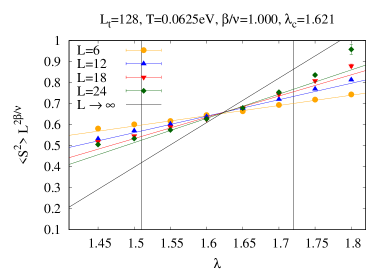
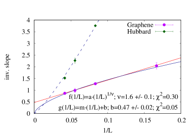
Figure 6: Figures taken from [6]. Left: Finite size scaling of $\langle S^{2}\rangle$ for graphene with fixed $\beta/\nu=1.0$. Linear fits bounded by vertical lines. Right: Extrapolation of the inverse slope of the fits to $L=\infty$ limit, using $g(1/L)=m\cdot(1/L)+b$ and $f(1/L)=a\cdot(1/L)^{1/\nu}$ respectively, where $\nu$ is a free parameter. $g(\cdot)$ (with smaller $\chi^{2}$) predicts that the slope remains finite for $L\to\infty$, suggesting that the data collapse onto a universal function without a rescaling of $\lambda$. Results for the Hubbard model with a power-law model curve shown for comparison.

To test this we fixed $\beta/\nu=1$ and plotted $\langle S^{2}\rangle L^{2\beta/\nu}$ over $\lambda$ (see figure 6, left panel). We find linear fits to the data intersect at around $\lambda\approx 1.62$, which is consistent within error with $\lambda_{c}=1.61\pm 0.02$ obtained from the fits to (20) discussed above. More importantly, we note that the slopes in the intersection plot do not appear to increase towards infinity with increasing volumes as they should for a second-order phase transition. This is consistent with $\nu\to\infty$, as it would imply a collapse of all data without a rescaling of the coupling constant. To investigate this somewhat more carefully, we plot the inverse slopes of our linear fits to $\langle S^{2}\rangle L^{2\beta/\nu}$ from the intersection plots over $1/L$ in the right panel of figure 6: While test data for the Hubbard model once again shows the expected behavior, the inverse slopes for graphene (with $\beta/\nu=1.0$) are well described by a linear model fit to

$$g(1/L)=m\cdot(1/L)+b\quad\mbox{with}\quad b=0.47\pm 0.02\,.$$

This non-zero intercept $b$ then provides our best numerical evidence of a finite slope in the infinite-volume limit and hence of $\beta,\nu\to\infty$ as CPT characteristics.

5 Lifshitz transition in graphene

In the electronic bands of the non-interacting tight-binding theory one finds saddle points, located at the M-points, which are characterized by a vanishing group velocity (see left panel of figure 7 for an illustration of the band structure). These separate the low-energy region, described by an effective Dirac theory, from a region where electronic quasi-particles behave like a regular Fermi liquid with a parabolic dispersion relation centered around the $\Gamma$-points. When the Fermi level is shifted across the saddle points by a chemical potential $\mu$, a change of the topology of the Fermi surface (which is one-dimensional for a 2D crystal) takes place. The distinct circular Fermi (isofrequency) lines surrounding the Dirac points are deformed into triangles, meet to form one large connected region and then break up again into circles around the $\Gamma$-points (see figure 7, right). This is known as neck-disrupting Lifshitz transition (NDLT) and occurs exactly at $\mu=\kappa$ (where $\kappa$ is the hopping energy) in the non-interacting theory. It also leads to a logarithmic divergence of the peak height of the density-of-states (DOS) with increasing surface area of the graphene sheet, known as a van Hove singularity (VHS).

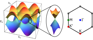
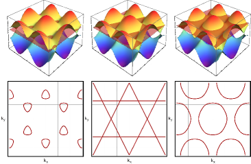
Figure 7: Figures taken from [7]. Left: Band structure of tight-binding theory of graphene. Dirac cones around the K-points are enlarged. The first Brillouin zone and terminology for special points are shown. Right: Topology of the Fermi lines (intersection lines with horizontal planes) for Fermi levels below (left), exactly at (middle) and above (right) the saddle points.

The Lifshitz transition is not a true phase transition in the thermodynamic sense, as it is purely topological and not associated with any type of symmetry breaking. Since interactions are strongly enhanced by the divergent DOS, it is generally believed however that the VHS is unstable towards formation of electronic ordered phases if many-body interactions are accounted for. This would imply that the Lifshitz transition becomes a true phase transition in a realistic description of the interacting system at low temperatures. An exciting possibility is the emergence of an anomalous time-reversal symmetry violating chiral d-wave superconducting phase in graphene [24]. In light of the recent discovery of a tunable superconducting gap in twisted bilayer graphene, which exists only for certain “magic” twist angles [25], there is also renewed interest in the VHS, as a possible driving-mechanism for this instability [26].

In [7] we studied the fate of the VHS in the presence of interactions at finite spin density using HMC. This was done by adding a Zeeman-splitting term to the Hamiltonian, which shifts the Fermi levels of the two spin orientations in opposite directions. In the non-interacting limit, finite spin and finite charge density are indistinguishable, and either one may be used to characterize the NDLT. Unlike finite charge density, simulations at finite spin density are not affected by a fermion sign problem and allow us to probe genuine interaction effects on the VHS. Physically, our setup corresponds to an in-plane magnetic field, which is interesting in its own right. Simulations were carried out using the linearized fermion matrix, purely imaginary Hubbard fields, and a spin-staggered mass term of $m_{s}=0.5\,\textrm{eV}$ to remove zero modes. We used the same partially screened Coulomb potential as discussed in section 4, with a rescaling parameter $\lambda$ to control the interaction strength.

The logarithmic divergence of the DOS is manifest only at $T=0$ and is inaccessible to our simulations. Instead, we thus focused on the ferromagnetic susceptibility $\chi$, which is related to the DOS through the polarization or Lindhard function and can also be used to characterize the NDLT (see [7] for a detailed discussion). $\chi(\mu)$ is given by

$$\chi(\mu) =-\frac{1}{N_{c}}\,\left(\frac{d^{2}\Phi}{d\mu^{2}}\right)=\frac{1}{N_{c}\beta}\left[\frac{1}{Z}\frac{d^{2}Z}{d\mu^{2}}-\frac{1}{Z^{2}}\left(\frac{dZ}{d\mu}\right)^{2}\right]~{},$$ (22)

where $\Phi=-T\ln{Z}$ is the grand-canonical potential and $N_{c}=N^{2}$ is the number of unit cells. From this we can obtain $\chi=\chi_{\mathrm{con}}+\chi_{\mathrm{dis}}$, with

$$\chi_{\mathrm{con}}(\mu) = \frac{-2}{N_{c}\beta}\left\langle\textrm{ReTr}\left(M^{-1}\frac{dM}{d\mu}M^{-1}\frac{dM}{d\mu}\right)\right\rangle,~{}$$ (23)

$$\chi_{\mathrm{dis}}(\mu) = \frac{4}{N_{c}\beta}\left\{\left\langle\left[\textrm{ReTr}\left(M^{-1}\frac{dM}{d\mu}\right)\right]^{2}\right\rangle-\left\langle\textrm{ReTr}\left(M^{-1}\frac{dM}{d\mu}\right)\right\rangle^{2}\right\},$$ (24)

where $\chi_{\mathrm{con/dis}}$ denote the connected and disconnected contributions respectively. At any non-zero temperature, the infinite volume limit of $\chi(\mu)$ is bounded from above by some value $\chi_{\mathrm{max}}$, which diverges as the temperature is lowered. In the non-interacting theory, this divergence occurs exactly at $\mu=\kappa$ and is described by

$$\chi_{\mathrm{max}}(T,\mu=\kappa)=-\frac{3g_{\sigma}}{2\pi^{2}\kappa}\ln{\big{(}{\pi T}/{\kappa}\big{)}}+\gamma_{E}+3\ln 2+\mathcal{O}(T)~{},$$ (25)

where $\gamma_{E}$ is the Euler-Mascheroni constant and $g_{\sigma}=2$ for the spin degeneracy. In this limit $\chi_{\mathrm{dis}}$ vanishes exactly since the expectation value $\langle\mathrm{ReTr}(\ldots)^{2}\rangle$ factorizes, and hence the divergence is driven purely by the connected part.

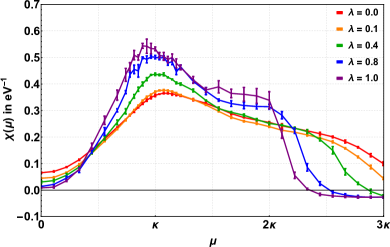
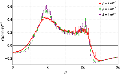
Figure 8: Figures taken from [7]. Left: $\chi(\mu)$ for $\beta=2\textrm{ eV}^{-1}$, $N=12$ at different interaction strengths. All points are quadratic $\delta_{\tau}\rightarrow 0$ extrapolations from simulations at non-zero $\delta_{\tau}$. Right: Temperature dependence of $\chi(\mu)$. Lattice sizes scale linearly with $\beta$, such that the displayed curves correspond to $N=12,18,24$ respectively; with $\delta_{\tau}=1/6~{}\textrm{eV}^{-1}$ and $\lambda=1$ for all cases.

In figure 8 (left) we show $\chi(\mu)$ with $N=12$ at different interaction strengths, ranging from the non-interacting theory to suspended graphene. These calculations were done at fixed temperature with $\beta=2\textrm{ eV}^{-1}$ (to set the energy scale we chose a hopping parameter of $\kappa=2.7\textrm{ eV}$ here, which roughly corresponds to the experimental value of graphene). Each point was obtained from simulations at several values of $\delta_{\tau}$ and extrapolated to the limit $\delta_{\tau}\rightarrow 0$ using quadratic polynomials. We observe that the peak at the VHS becomes more and more pronounced with increasing interaction strength. This is due to both, a corresponding rise in the connected part at the VHS and an additional contribution from the disconnected part. Likewise, the peak position as well as the upper end of the conduction band are shifted towards smaller values of $\mu$. Our results are in qualitative agreement with experimental data from angle resolved photoemission spectroscopy (ARPES) measurements on charge-doped graphene systems, which show evidence for a warping of the Fermi surface, leading to an extended, not pointlike, van Hove singularity characterized by the flatness of the bands along one direction, and hence a stronger divergence of the DOS than in the non-interacting system [27]. Such experiments also observed bandwidth renormalization (narrowing of the widths of the $\pi$-bands), due to interactions and doping [28].

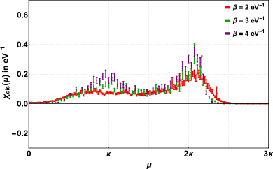
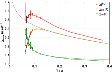
Figure 9: Figures taken from [7]. Left: Temperature dependence of $\chi_{\mathrm{dis}}(\mu)$. Lattice sizes scale linearly with $\beta$, such that the displayed curves correspond to $N=12,18,24$ respectively; with $\delta_{\tau}=1/6~{}\textrm{eV}^{-1}$ and $\lambda=1$ for all cases. Right: Temperature dependence of $\chi_{\mathrm{max}}$ in the range $\beta=1.0,\ldots 6.0\textrm{ eV}^{-1}$. Dotted lines are fits using (26) for $\chi_{\mathrm{con}}^{\mathrm{max}}$ and (27) for $\chi_{\mathrm{dis}}^{\mathrm{max}}$ in appropriate ranges (see text).

In figure 8 (right) we show the temperature dependence of $\chi(\mu)$ for suspended graphene ($\lambda=1$). Here we chose a fixed time-discretization of $\delta_{\tau}=1/6~{}\textrm{eV}^{-1}$, which produces a nearly constant negative shift of $\chi$ (with only a very weak dependence on $\mu$) as the leading discretization effect. Lattice sizes scale with $\beta$ such that the infinite volume limit is obtained in each case. This requires larger systems at smaller temperatures, such that the displayed curves correspond to $N=12,18,24$ respectively. Here we again observe a stronger peak at $\mu\approx\kappa$, which grows as the temperature is lowered. What is striking is that this increase receives sizable contributions from the disconnected part (shown in figure 9, left), which is also unaffected by negative offsets from the Euclidean time discretization.

Figure 9 (right) shows the temperature dependence for the peak heights of $\chi/\chi_{\mathrm{con}}/\chi_{\mathrm{dis}}$. We have identified a range of $\beta=1/T$ between $1.0$ eV^-1 and $3.0$ eV^-1 where a fit of the form

$$f_{1}(T)=a\ln\left(\frac{\kappa}{T}\right)+b+c\,\frac{T}{\kappa}$$ (26)

to the full susceptibility is possible (it breaks down if one attempts to include lower temperatures). More interestingly, however, the same fit to $\chi_{\mathrm{con}}$ alone is consistent with $a=3/(\pi^{2}\kappa)$ for $\beta\leq 2.5$ eV^-1, and thus basically fully agrees with the non-interacting tight-binding model. At temperatures below $T\sim 0.15\,\kappa$ the contribution from $\chi_{\mathrm{con}}$ suddenly drops however. This is contrasted by a rapid increase of the peak height of $\chi_{\mathrm{dis}}$. While $\chi_{\mathrm{dis}}$ is negligible at high temperatures, it becomes the dominant contribution at $T\sim 0.07\,\kappa$. In fact, we find that for $\beta\geq 2.5\textrm{ eV}^{-1}$ (corresponding to $T\leq 0.15\,\kappa$), $\chi_{\mathrm{dis}}^{\mathrm{max}}$ is well described by the model

$$f_{2}(T)=k\left|\frac{T-T_{c}}{T_{c}}\right|^{-\gamma}~{},$$ (27)

with $\beta_{c}=6.1(5)\,\textrm{eV}^{-1}$ and $\gamma=0.52(6)$. The emerging peak in $\chi^{\mathrm{max}}_{\mathrm{dis}}(T)$ around $\beta\approx 6$ eV^-1 is thus consistent with a power-law divergence indicative of a thermodynamic phase transition at non-zero $T_{c}$. All attempts to model $\chi_{\mathrm{dis}}^{\mathrm{max}}(T)$ using a logarithmic increase as in (26) were unsuccessful, so that our conclusion seems qualitatively robust.

6 Graphene with hydrogen adatoms

Functionalization of graphene with hydrogen or other adatoms is a subject of interest, as it provides a way to create a tunable band gap in graphene or to control its magnetic properties. The spatial distribution of adatoms thereby plays a crucial role, with the question of stability (or instability) of adatom superlattices or other configurations being of central importance. The smallness of the pairwise elastic interactions of hydrogen adatoms in graphene suggests that the Ruderman-Kittel-Kasuya-Yosida (RKKY) contribution from conduction electrons dominates the inter-adatom interactions. The influence of electron-electron interactions on these is quite strong in graphene, but is difficult to study quantitatively with Density Functional Theory or similar methods.

In [8] we carried out a HMC study of the RKKY interaction between hydrogen adatoms in graphene, consistently taking into account inter-electron interactions. In the interacting tight-binding model the RKKY interaction is simply the fermionic Casimir potential. For a pair of adatoms we calculate it as the free energy $\mathcal{F}_{xy}$ of the electrons on the graphene lattice with adatoms at sites $x$ and $y$. In absence of inter-electron interactions we can simply compute the corresponding single-particle energy levels $\epsilon_{xy}$ with adatoms and obtain $\mathcal{F}_{xy}$ up to an irrelevant constant $F_{0}$ from

$$\mathcal{F}_{xy}=-T\sum_{\epsilon_{xy}}\ln\left(1+e^{-\epsilon_{xy}/T}\right)+F_{0}~{}.$$ (28)

With interactions, we instead calculate the differences $\Delta\mathcal{F}=\mathcal{F}_{x+l,y}-\mathcal{F}_{x,y}$ between free energies for adatom positions which differ by a shift along one carbon-carbon lattice bond $l$, which we represent as

$$\Delta\mathcal{F}=-T\int_{0}^{1}d\alpha\,\partial_{\alpha}\,\log\mathcal{Z}_{\alpha},\quad\mathcal{Z}_{\alpha}=\int\mathcal{D}\phi_{x,\tau}\,e^{-S\left[\phi_{x,\tau}\right]}|{\rm det}\left(M_{\alpha}\left[\phi_{x,\tau}\right]\right)|^{2}.$$ (29)

Here $M_{\alpha}$ linearly interpolates between fermionic operators with adatoms at positions $x$ and $y$ (at $\alpha=0$) and $x+l$ and $y$ (at $\alpha=1$). Differentiating the path integral (29) for $\mathcal{Z}_{\alpha}$ by $\alpha$, we obtain

$$\Delta\mathcal{F}=-2T\int_{0}^{1}d\alpha\,\langle\,{\rm Re}\,\tr\left(M_{\alpha}^{-1}\partial_{\alpha}M_{\alpha}\right)\,\rangle.$$ (30)

The integral over $\alpha$ is calculated using the 6-point quadrature rule. The above is easily extended to more than two adatoms.

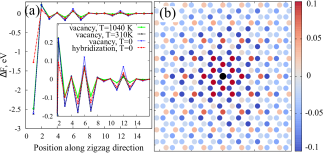
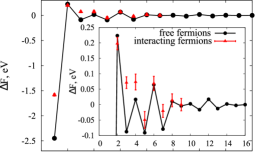
Figure 10: Figures taken from [8]. Left: Interaction of two adatoms in free tight-binding model on $72\times 72$ lattice. (a) profile along zigzag direction (zoomed version in the inset); (b) 2D profile of RKKY potential for non-interacting hybridization model at $T=310\,{\rm K}$. Right: Pairwise RKKY interaction in the interacting tight-binding model compared with non-interacting case. Zoomed version in the inset. Adatoms were modeled as vacancies.

We used two models of hydrogen adatoms: A simple vacancy model describing hydrogen adatoms as missing lattice sites, and the full hybridization model, in which hybridization terms are added to the Hamiltonian. As the hybridization model suffers from a sign problem, we use it only in the non-interacting limit. It is used, among other things, to verify the validity of the vacancy model and in cases where the effect of interactions can be modeled by SDW or CDW mass terms. In figure 10 (left) we demonstrate that, without inter-electron interactions, the RKKY potentials are very similar for both models. In all cases the pairwise RKKY interaction has well-known features: alternating signs for different sublattices and an order-of-magnitude enhancement at some distances, at which the two adatoms induce midgap states with zero energy. We also demonstrate that relatively high temperatures of $T=1040\,{\rm K}$ do not affect these qualitative features.

In figure 10 (right) we illustrate the effect of inter-electron interactions on the RKKY potential along the zigzag direction using the vacancy model. The potential is particularly strongly modified at distances of 3 and 4 C-C bonds, while at distances larger then 8-9 C-C bonds the change of potential is too small to detect it with HMC. The main physical effect is that the local minimum at a distance of 3 bonds disappears and the potential barrier between widely separated adatoms and the global minimum corresponding to a dimer configuration becomes harder to penetrate.

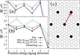
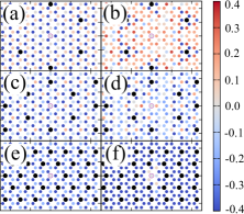
Figure 11: Figures taken from [8]. Left: Free energy change of the superlattice system (vacancy model) upon displacement of a single adatom for $L=24$, $T=0.09\,{\rm eV}$ (zoom-in and overview); (c) superlattice structure with the zigzag profile used in figures (a) and (b) indicated by the red arrow. Right: Change of free energy of superlattice systems upon the displacement of a single adatom. The fixed positions of other adatoms in the superlattices are marked with black dots. All plots correspond to the non-interacting hybridization model with SDW mass term at half-filling.

We analyzed the stability of several regular adatom superlattices with respect to small displacements of a single adatom. Figure 11 (left) shows one such system, with $5.56\%$ coverage of hydrogen adatoms populating only one sublattice, which is the case we studied in most detail. Here the vacancy model is used in both the interacting and non-interacting case (to avoid a sign problem for the former and make a direct comparison meaningful). The overall scale of the RKKY interaction is enhanced in comparison with pairwise interaction. Inter-electron interactions do not change the RKKY potential qualitatively, despite inducing a very large gap $\Delta\epsilon\sim 1\textrm{eV}$ in the midgap energy band, and are modelled quite accurately by adding a SDW mass term to the non-interacting tight-binding theory. A CDW mass term on the other hand completely changes the RKKY potential and the locations of its minima.

We also addressed the dynamic stability of superlattice configurations with only one or both sublattices populated by adatoms, by using the hybridization model without inter-electron interactions but with a SDW mass term. Results are shown in figure 11 (right). We observe that the superlattices with adatoms on a single sublattice at half filling are dynamically unstable in all cases considered, due to fact that a change of position of an adatom to the opposite sublattice is energetically favourable. In contrast, superlattices of adatoms which equally populate both sublattices are stable for low adatom concentration. Single-sublattice superlattices can be stabilized by a chemical potential. This was also studied in [8]. The main conclusion is that a larger density of adatoms requires a larger chemical potential to stabilize it.

7 Outlook

In conclusion, we note that there are of course several directions to continue each of the projects presented here. The CPT scenario in graphene should certainly be tested on larger system sizes, and the precise role of the short- and long-range parts of the inter-electron potential investigated further. In particular, it would be instructive to repeat the analysis of section 4 for the case of unscreened Coulomb interactions.

At the VHS one should study the competition between different ordered phases, in particular of superconducting condensates, which can be expressed in a Nambu-Gorkov basis. Genuine simulations at finite charge density are prevented by a sign problem, but may be possible for small values of the chemical potential. In this context, recently much progress has been made in applying the Lefschetz thimble decomposition to the repulsive Hubbard model [29, 30, 31]. We are also in the process of adapting the Linear Logarithmic Relaxation method [32], which generalizes the Wang-Landau algorithm to systems with continuous degrees of freedom, to the repulsive Hubbard model away from half filling [33].

We note that the chiral Gross-Neveu model is interesting in its own right, as an effective theory for chiral symmetry breaking in relativistic field theories, where it is better known as the Nambu-Jona-Lasinio (NJL) model. In $2+1$ spacetime dimensions, the attractive Hubbard model on the honeycomb lattice (which can be simulated at finite charge density without a sign problem) defines a discretization of this theory similar to the Creutz-Borici action (which describes two degenerate flavors of chiral fermions, the minimum number allowed by the Nielsen-Ninomiya theorem), but which avoids discretization errors produced by a vector-like anisotropy, typical for “minimally doubled” fermionic actions on hypercubic lattices. This could be useful in the future e.g. to test the stability of inhomogeneous chiral condensates beyond the mean-field level.

Finally, we point out that there are a great number of additional Hubbard-type models of interest in condensed matter physics, which might possibly be targets for future HMC studies. At present much attention is paid, for instance, to systems with flat bands in the spectrum, such twisted bilayer graphene [25] or pseudospin-1 fermions on a dice lattice [34] (flat bands can also contribute to RKKY interactions [35]). Many such models might either be free of a fermion sign problem from the outset, or exhibit a sign problem which turns out to be mild upon closer inspection, and hence tractable through various techniques. A detailed survey of such models is definitely of interest, but is beyond the scope of this work.

References

References

- [1] Bermudez A, Goldman N, Kubasiak A, Lewenstein M and Martin-Delgado M A 2010 New Journal of Physics 12 033041 URL https://iopscience.iop.org/article/10.1088/1367-2630/12/3/033041
- [2] Mazza L, Bermudez A, Goldman N, Rizzi M, Martin-Delgado M A and Lewenstein M 2012 New Journal of Physics 14 015007 URL https://iopscience.iop.org/article/10.1088/1367-2630/14/1/015007
- [3] Wehling T O, Şaşıoğlu E, Friedrich C, Lichtenstein A I, Katsnelson M I and Blügel S 2011 Phys. Rev. Lett. 106(23) 236805 URL https://link.aps.org/doi/10.1103/PhysRevLett.106.236805
- [4] Koshino M, Yuan N F Q, Koretsune T, Ochi M, Kuroki K and Fu L 2018 Phys. Rev. X 8(3) 031087 URL https://link.aps.org/doi/10.1103/PhysRevX.8.031087
- [5] Buividovich P, Smith D, Ulybyshev M and von Smekal L 2018 Phys. Rev. B 98(8) 235129 URL https://link.aps.org/doi/10.1103/PhysRevB.80.98.235129
- [6] Buividovich P, Smith D, Ulybyshev M and von Smekal L 2019 Phys. Rev. B 99(20) 205434 URL https://link.aps.org/doi/10.1103/PhysRevB.99.205434
- [7] Körner M, Smith D, Buividovich P, Ulybyshev M and von Smekal L 2017 Phys. Rev. B 96(19) 195408 URL https://link.aps.org/doi/10.1103/PhysRevB.96.195408
- [8] Buividovich P, Smith D, Ulybyshev M and von Smekal L 2017 Phys. Rev. B 96(16) 165411 URL https://link.aps.org/doi/10.1103/PhysRevB.96.165411
- [9] Brower R C, Rebbi C and Schaich D 2011 PoS Lattice2011 056 (Preprint 1204.5424)
- [10] Hirsch J E 1985 Phys. Rev. B 31(7) 4403–4419 URL https://link.aps.org/doi/10.1103/PhysRevB.31.4403
- [11] Blankenbecler R, Scalapino D J and Sugar R L 1981 Phys. Rev. D 24(8) 2278–2286 URL https://link.aps.org/doi/10.1103/PhysRevD.24.2278
- [12] Smith D and von Smekal L 2014 Phys. Rev. B 89(19) 195429 URL https://link.aps.org/doi/10.1103/PhysRevB.89.195429
- [13] Buividovich P, Smith D, Ulybyshev M and von Smekal L 2016 PoS Lattice2016 244 URL https://doi.org/10.22323/1.256.0244
- [14] Luu T and Lähde T A 2016 Phys. Rev. B 93(15) 155106 URL https://link.aps.org/doi/10.1103/PhysRevB.93.155106
- [15] Assaad F F and Herbut I F 2013 Phys. Rev. X 3(3) 031010 URL https://link.aps.org/doi/10.1103/PhysRevX.3.031010
- [16] Otsuka Y, Yunoki S and Sorella S 2016 Phys. Rev. X 6(1) 011029 URL https://link.aps.org/doi/10.1103/PhysRevX.6.011029
- [17] Parisen Toldin F, Hohenadler M, Assaad F F and Herbut I F 2015 Phys. Rev. B 91(16) 165108 URL https://link.aps.org/doi/10.1103/PhysRevB.91.165108
- [18] Classen L, Herbut I F, Janssen L and Scherer M M 2016 Phys. Rev. B 93(12) 125119 URL https://link.aps.org/doi/10.1103/PhysRevB.93.125119
- [19] Semenoff G W 2012 Physica Scripta T146 014016 URL https://doi.org/10.1088%2F0031-8949%2F2012%2Ft146%2F014016
- [20] Herbut I F 2006 Phys. Rev. Lett. 97(14) 146401 URL https://link.aps.org/doi/10.1103/PhysRevLett.97.146401
- [21] Gamayun O V, Gorbar E V and Gusynin V P 2010 Phys. Rev. B 81(7) 075429 URL link.aps.org/doi/10.1103/PhysRevB.81.075429
- [22] Buividovich P V and Polikarpov M I 2012 Phys. Rev. B 86(24) 245117 URL https://link.aps.org/doi/10.1103/PhysRevB.86.245117
- [23] Ulybyshev M V, Buividovich P V, Katsnelson M I and Polikarpov M I 2013 Phys. Rev. Lett. 111(5) 056801 URL https://link.aps.org/doi/10.1103/PhysRevLett.111.056801
- [24] Nandkishore R, Levitov L and Chubukov A 2012 Nature Phys. 8 158–163 URL https://www.nature.com/articles/nphys2208
- [25] Cao Y, Fatemi V, Fang S, Watanabe K, Taniguchi T, Kaxiras E and Jarillo-Herrero P 2018 Nature 556 43–50 URL https://doi.org/10.1038/nature26160
- [26] Sherkunov Y and Betouras J J 2018 Phys. Rev. B 98(20) 205151 URL https://link.aps.org/doi/10.1103/PhysRevB.98.205151
- [27] McChesney J L, Bostwick A, Ohta T, Seyller T, Horn K, González J and Rotenberg E 2010 Phys. Rev. Lett. 104(13) 136803 URL https://link.aps.org/doi/10.1103/PhysRevLett.104.136803
- [28] Ulstrup S, Schüler M, Bianchi M, Fromm F, Raidel C, Seyller T, Wehling T and Hofmann P 2016 Phys. Rev. B 94(8) 081403 URL https://link.aps.org/doi/10.1103/PhysRevB.94.081403
- [29] Ulybyshev M V and Valgushev S N 2017 (Preprint 1712.02188)
- [30] Ulybyshev M, Winterowd C and Zafeiropoulos S 2019 (Preprint 1906.07678)
- [31] Ulybyshev M, Winterowd C and Zafeiropoulos S 2019 (Preprint 1906.02726)
- [32] Langfeld K, Lucini B and Rago A 2012 Phys. Rev. Lett. 109(11) 111601 URL https://link.aps.org/doi/10.1103/PhysRevLett.109.111601
- [33] Körner M, Langfeld K, Smith D and von Smekal L 2020 Phys. Rev. D 102(5) 054502 URL https://link.aps.org/doi/10.1103/PhysRevD.102.054502
- [34] Raoux A, Morigi M, Fuchs J N, Piéchon F and Montambaux G 2014 Phys. Rev. Lett. 112(2) 026402 URL https://link.aps.org/doi/10.1103/PhysRevLett.112.026402
- [35] Oriekhov D O and Gusynin V P 2020 Phys. Rev. B 101(23) 235162 URL https://link.aps.org/doi/10.1103/PhysRevB.101.235162