Bayesian estimation of large dimensional time varying VARs using copulas

Abstract

This paper provides a simple, yet reliable, alternative to the (Bayesian) estimation of large multivariate VARs with time variation in the conditional mean equations and/or in the covariance structure. With our new methodology, the original multivariate, $n$-dimensional model is treated as a set of $n$ univariate estimation problems, and cross-dependence is handled through the use of a copula. Thus, only univariate distribution functions are needed when estimating the individual equations, which are often available in closed form, and easy to handle with MCMC (or other techniques). Estimation is carried out in parallel for the individual equations. Thereafter, the individual posteriors are combined with the copula, so obtaining a joint posterior which can be easily resampled. We illustrate our approach by applying it to a large time-varying parameter VAR with $25$ macroeconomic variables.

1 Introduction

Following the seminal contributions by Sims (1980) and Litterman (1986), Vector AutoRegression (VAR) models and their variants are now ubiquitously applied to multivariate time series, as a flexible alternative to structural models. There is now a huge body of literature on both theory and applications: useful surveys are provided inter alia by Watson (1994) and Lütkepohl (2005).
Although in their standard form VARs already offer a relatively flexible modelling approach, extensions have been considered to accommodate time variation. This may occur in the coefficients of the conditional mean equations (see e.g. Doan et al., 1984; Canova, 1993; Sims, 1993; Stock and Watson, 1996; and Cogley and Sargent, 2001), so affording a flexible alternative to models with abrupt breaks, known as the Time-Varying Parameter VAR (TVP-VAR). Time variation has also been considered in the covariance matrix of the error term, thereby allowing for time-varying heteroskedasticity. Following seminal papers by Uhlig (1997), Cogley and Sargent (2001) and Primiceri (2005), recent examples where the assumption of homoskedasticity has been relaxed include Koop and Korobilis (2013) and Koop et al. (2019), who attempt to reduce the dimensionality issue essentially by imposing a factor structure onto the volatilities - see also Clark (2011), Carriero et al. (2015), Clark and Ravazzolo (2015) and Carriero et al. (2016). In a recent landmark paper, Carriero et al. (2019) propose a far less restrictive set-up, which allows for fully Bayesian inference without imposing restrictions on the form of the heteroskedasticity.

Across the extensive literature on multivariate models, virtually all studies have one issue in common: the dimensionality of the model and the computational burden it brings about. On the one hand, unless the number of variables involved in the model is relatively large, omitted variable bias may impair the forecasting ability of the model (see Giannone and Reichlin, 2006). Carriero et al. (2019) make a compelling case for the superior performance of large dimensional VARs. On the other hand, computational difficulties may arise when there are a large number of variables and, more substantially, over-parameterisation can occur. Thus, the literature has focused on finding techniques that allow for the estimation of large VARs: see Bańbura et al. (2010) for an excellent review of the various approaches which have been proposed. In the case of homoskedastic VARs, the dimensionality issue can be handled by the choice of appropriate (conjugate) prior distributions, as shown by Bańbura et al. (2010) who successfully apply their technique to the estimation of a VAR with 130 variables. Conversely, in the case of a heteroskedastic VAR, this is no longer possible, and the computational burden cannot be resolved through the choice of an appropriate prior. As explained in Carriero et al. (2019), heteroskedasticity invalidates the so-called “symmetry”across equations that characterises homoskedastic VARs. Such property entails that a homoskedastic VAR is a SUR model where the regressors are the same across all equations; in turn, this entails that the covariance matrix of the VAR coefficients has a Kronecker structure, which makes estimation much simpler than if one had to deal with large matrices that do not have a simplifying structure. Few contributions consider estimation of a large VAR with time variation in both the coefficients of the conditional mean equations and of the covariance matrix of the error term. Koop and Korobilis (2013) and Koop et al. (2019) propose an estimation technique for large, possibly heteroskedastic TVP-VARs, which essentially relies on the Kalman filter. However, their approach is not fully Bayesian, and it is liable to mis-specification issues if the assumed model for coefficient variation is not correct, also being, in practice, limited in dealing with the dimensionality issues - we refer however to a recent contribution by Kapetanios et al. (2019) which, through a non-parametric approach, solves these issues. Carriero et al. (2019) solve the problem of fully Bayesian estimation of large VARs with heterskedasticity, by proposing a new estimation algorithm which is shown to perform very well in out-of-sample forecasting and also in structural analysis. However, their paper does not consider the presence of time varying coefficients in the VAR specification.

Proposed methodology and main contribution of this paper

This paper proposes a copula-based Bayesian estimation methodology for large TVP-VARs with heteroskedasticity. Similarly to Carriero et al. (2019), our estimators are fully Bayesian, thus allowing for the computation of the uncertainty around all estimators.
Full details of our approach are in Section 2; here, we give a heuristic preview of our methodology. Given a multivariate model of (possibly) very large dimension $n$, we reduce it into $n$ univariate models, which are more easily handled. In order to recover the cross-dependence among equations, we use a copula-like term. In consequence, the likelihood function in our system factors into the likelihoods of the individual autoregressive models, plus the likelihood of the copula term. Thereby we are able to obtain a posterior where each set of parameters (the $n$ sets corresponding to the $n$ equations, and the set corresponding to the copula) is, conditional on the sample, independently distributed of the other sets. Therefore, from a computational point of view, each univariate problem is dealt with separately, which greatly reduces the computational burden. In this respect, our idea of breaking down the multivariate estimation problem into separate univariate problems is similar to the approach for fixed parameter, homoskedastic VARs developed in Korobilis and Pettenuzzo (2019), although in our case we allow for time variation in the conditional mean and variance. The use of copulas to model dependence has also been considered by the literature in a Bayesian context (see e.g. Gruber and Czado, 2015 and Gruber and Czado, 2018), including non-parametric Bayesian analysis (we refer, inter alia, to the contributions by Rodriguez and ter Horst (2008), Taddy (2010), Nieto-Barajas et al. (2012), Di Lucca et al. (2013), Bassetti et al. (2014) and Nieto-Barajas and Quintana (2016)).
Our approach allows for great flexibility in the specification of the univariate models. For example, in the simplest version of our methodology, each series is modelled as an AR(1) model. However, given that more sophisticated model selection tools may be desirable to construct the univariate models, we develop an approach based on a model selection technique known as Bayesian compression (see Guhaniyogi and Dunson, 2015). Moreover, whilst the focus of this paper in on TVP-VARs with heteroskedasticity, our approach can be also used to estimate other multivariate models such as e.g. VARMAs and Multivariate Stochastic Volatility models (MSV). In particular, in appendix we carry out an empirical exercise using VARMAs, to illustrate the computational convenience of our approach. Also, in another contribution (Tsionas et al., 2019), we apply our methodology to large MSV models for financial variables. Here, we illustrate our methodology by estimating a large TVP-VAR model with possible heteroskedasticity, using the same data as Koop and Korobilis (2013).

The remainder of the paper is organised as follows. Our methodology is spelt out in Section 2. The empirical application is in Section 3; we also report a further application to VARMAs in Appendix B. Section 4 concludes.

2 Methodology

We begin by introducing the main model and some notation. We consider the TVP-VAR($p$)

$$\mathbf{y}_{t}=\sum_{j=1}^{p}A_{t,j}\mathbf{y}_{t-j}+\mathbf{u}_{t},\text{ \ \ }p+1\leq t\leq T,$$ (2.1)

where $\mathbf{y}_{t}$ is an $n\times 1$ vector and $\mathbf{u}_{t}$ is a zero mean, Gaussian process with possibly time varying variance - we discuss the specification of the second moment later on. Model (2.1) could be extended to consider e.g. exogenous regressors, latent regressors such as common factors, or deterministics such as a constant, (linear or nonlinear) trends and seasonal dummies. Also, (2.1) could also have an MA($q$) structure, in the spirit of Chan et al. (2013); or it could have no autoregressive structure at all, and only time varying heteroskedasticity as in the case of Creal and Tsay (2015). We prefer to focus on a simpler specification, so that the discussion is not overshadowed by the algebra. Similarly, the assumption that $\mathbf{u}_{t}$ is Gaussian is made only for simplicity. Note that, even in this simple set-up, the number of parameters grows rapidly with $p$ and $n$, whence the dimensionality issue.

2.1 Theory: the univariate equations, the copula and the likelihood function

The univariate equations

In the context of (2.1), we consider the following univariate AR($p$) models

$$y_{i,t}=\sum_{j=1}^{p}\beta_{i,t,j}y_{i,t-j}+u_{i,t}=\beta_{i,t}^{\left(1\right)\prime}z_{i,t}^{\left(1\right)}+u_{i,t},$$ (2.2)

for $1\leq i\leq n$ with $u_{i,t}=e^{h_{i,t}/2}u_{i,t}^{*}$, where $u_{i,t}^{\ast}\sim i.i.d.N(0,1)$ and

$$h_{i,t}=\alpha_{i}+\gamma_{i}h_{i,t-1}+e_{i,t},$$ (2.3)

with $e_{i,t}\sim i.i.d.N(0,\delta_{i})$. As noted above, (2.2) can be extended and/or modified to incorporate e.g. a different number of lags $p_{i}$ for each unit, an MA($q_{i}$) component, exogenous regressors, deterministics, (conditional or unconditional) heteroskedasticity, etc.. Similarly, (2.3) could be replaced e.g. by a GARCH specification to allow for conditional heteroskedasticity (see also the discussion in Uhlig, 1997 on the relative merits of possible specifications for time heteroskedasticity).

Given that in (2.2) $y_{i,t}$ is predicted using only its own past, this may lead to a loss of predictive accuracy. A possible alternative would be to use the Bayesian compression algorithm developed in Guhaniyogi and Dunson (2015). In particular, we consider the specification

$$y_{i,t}=\beta_{i,t}^{\left(2\right)\prime}z_{i,t}^{\left(2\right)}+u_{i,t},$$ (2.4)

with $u_{i,t}$ still satisfying (2.3). As in (2.2), $z_{i,t}^{\left(2\right)}$ is a subset of the regressors in each equation of the unrestricted VAR (say $\widetilde{z}_{i,t}$). However, in the case of (2.4), the vector $z_{i,t}^{\left(2\right)}$ can include lags of $y_{i,t}$ and also lags of $y_{j,t}$ for $j\neq i$. In order to select the components of $z_{i,t}^{\left(2\right)}$, Guhaniyogi and Dunson (2015) suggest the following technique. Let $z_{i,t}^{\left(2\right)}=\Phi\widetilde{z}_{i,t}$ with $\Phi$ a $p\times np$ matrix whose entries are defined as

$$\Phi_{ij}=\left\{\begin{array}[]{c}-\phi^{-1/2}\\ 0\\ \phi^{-1/2}\end{array}\right.\text{with probability }\begin{array}[]{c}\phi^{2}\\ 2\phi\left(1-\phi\right)\\ \left(1-\phi\right)^{2}\end{array},$$

and $\phi$ and $p$ are drawn uniformly from $\left(0.1,1\right)$ and $\left\{1,...,p^{\max}\right\}$, with $p^{\max}$ chosen so that the marginal likelihood has a global peak. The matrix $\Phi$ is then normalised via the Gram-Schmidt orthonormalisation - see Guhaniyogi and Dunson (2015) for details.

The copula

We now introduce the copula term to model dependence among the univariate equations. Letting $X$ denote a continuous $k$-dimensional random variable whose density is given by $f\left(x\right)$, it holds that

$$f\left(x\right)=\left(\prod\limits_{j=1}^{k}f_{j}\left(x_{j}\right)\right)c^{\ast}\left(v_{1},...,v_{k}\right),$$ (2.5)

where $f_{j}\left(x_{j}\right)$ is the density of the $j$-th coordinate of $X$, $v_{j}=F_{j}\left(x_{j}\right)=\int_{-\infty}^{x_{j}}f_{j}\left(u\right)du$, and $c^{\ast}\left(v_{1},...,v_{k}\right)$ is the copula density (which is unique since $X$ is continuous). This result is known as Sklar’s theorem (see Sklar, 1959 and Sklar, 1996; see also the book by Nelsen, 2007 for a comprehensive introduction to copulas). Equation (2.5) can equivalently be written as

$$\ln f\left(x\right)=\sum_{j=1}^{k}\ln f_{j}\left(x_{j}\right)+\ln c^{\ast}\left(v_{1},...,v_{k}\right).$$ (2.6)

The likelihood function

We now turn to specifying the likelihood. Henceforth, we use $z_{i,t}$ as short-hand for both $z_{i,t}^{\left(1\right)}$ and $z_{i,t}^{\left(2\right)}$; $\beta_{i,t}$ for both $\beta_{i,t}^{\left(1\right)}$ and $\beta_{i,t}^{\left(2\right)}$ in (2.2) and (2.4) respectively. We assume the following law of motion

$$\beta_{i,t}=A_{\beta,i}\beta_{i,t-1}+\epsilon_{i,t},$$ (2.7)

with $\epsilon_{i,t}\sim i.i.d.N\left(0,\Sigma_{i}\right)$, independent across $i$. We point out that, in (2.7), we do not impose the typical random walk model for the time-varying parameters (see e.g. Koop and Korobilis, 2013), which makes our set-up more general. For simplicity, we do not allow for time variation in any other parameter (i.e., we do not allow for the copula parameters, or the coefficients in (2.3), to vary over time).

Let $b_{i}=\left(\alpha_{i},\gamma_{i},\delta_{i}\right)$. Then, the marginal density of $y_{i,t}$ conditional on $z_{i,t}$ can be denoted as $f_{i}\left(y_{i,t}|z_{i,t};\beta_{i,t},b_{i}\right)$ (we omit dependence on $A_{\beta,i}$, $\Sigma_{i}$ and $\beta_{i,0}$ for short). Then, by (2.5), it holds that

$$f_{i}\left(\mathbf{y}_{t}|z_{t};\beta_{i,t},b_{i}\right)=\left(\prod\limits_{i=1}^{n}f_{i}\left(y_{i,t}|z_{i,t};\beta_{i,t},b_{i}\right)\right)c^{\ast}\left(v_{1,t},...,v_{n,t}\right),$$ (2.8)

having defined $v_{i,t}=\int_{-\infty}^{y_{i,t}}f_{i}\left(u|z_{i,t};\beta_{i,t},b_{i}\right)du$, with $f_{i}\left(u|z_{i,t};\beta_{i,t},b_{i}\right)$ denoting the density of $y_{i,t}$ conditional on $z_{i,t}$.

Although Sklar’s theorem ensures that the copula density $c^{\ast}\left(v_{1,t},...,v_{n,t}\right)$ is unique, it does not provide an expression for it. One possibility would be to consider a non-parametric copula, and we refer to Scaillet and Fermanian (2003), Ibragimov (2005) and Chen and Huang (2007), and the references therein, for the relevant theory in a time series context. In this paper, we choose a different set-up. In particular, we consider a (parametric) Gaussian mixture copula model (GMCM henceforth; see Tewari et al., 2011) model, viz.

$$c^{\ast}\left(v_{1,t},...,v_{n,t}\right)=\frac{\sum_{g=1}^{G}p_{g}f_{N}\left(\mathbf{y}_{t}|\mu_{g},\Omega_{g}\right)}{\prod_{g=1}^{G}p_{g}f_{N}\left(\mathbf{y}_{t}|\mu_{g},\Omega_{g}\right)}\equiv c\left(\mathbf{y}_{t}|\alpha\right),$$ (2.9)

where: $\left\{p_{g}\right\}_{g=1}^{G}$ (such that $\sum_{g=1}^{G}p_{g}=1$ and $p_{1}<...<p_{G}$) is a set of weights and $f_{N}\left(\cdot|\mu_{g},\Omega_{g}\right)$ is the density of an $n$-variate Gaussian random variable with mean $\mu_{g}$ and covariance matrix $\Omega_{g}$. In (2.9), we use the short-hand notation $\alpha=\left(\left(p_{1},...,p_{G}\right)^{\prime},\mu_{1}^{\prime},...,\mu_{G}^{\prime},\left(vech\left(\Omega_{1}\right)\right)^{\prime},...,\left(vech\left(\Omega_{G}\right)\right)^{\prime}\right)^{\prime}$.

Finally, let now $\beta_{t}=\left(\beta_{1,t}^{\prime},...,\beta_{n,t}^{\prime}\right)^{\prime}$, $\omega=\left(b_{1}^{\prime},...,b_{n}^{\prime}\right)^{\prime}$, $A_{\beta}=\left\{A_{\beta,1},...,A_{\beta,n}\right\}$, $\Sigma=\left\{\Sigma_{1},...,\Sigma_{n}\right\}$, and, for short,

$$\theta=\left(vec\left(\alpha\right)^{\prime},\omega^{\prime},vec\left(A_{\beta}\right)^{\prime},vech\left(\Sigma^{1/2}\right)^{\prime},vec\left(\beta_{0}\right)^{\prime}\right)^{\prime}.$$

Putting everything together, the resulting likelihood function (conditional on the initial observations $\left\{\mathbf{y}_{t}\right\}_{t=1}^{p}$) is given by

$$L\left(\left\{\mathbf{y}_{t}\right\}_{t=p+1}^{T}|\alpha,\omega,A_{\beta},\Sigma,\beta_{0},\left\{\beta_{t}\right\}_{t=1}^{T}\right) = L\left(\left\{\mathbf{y}_{t}\right\}_{t=p+1}^{T}|\theta,\left\{\beta_{t}\right\}_{t=1}^{T}\right)$$

$$= \prod\limits_{t=p+1}^{T}\left[\prod\limits_{i=1}^{n}f_{i}\left(y_{i,t}|z_{i,t};\beta_{i,t},A_{\beta,i},\Sigma_{i},\beta_{i,0},b_{i}\right)\right]c\left(\mathbf{y}_{t}|\alpha\right),$$

where we have now emphasized the dependence of the marginal densities on $A_{\beta,i}$, $\Sigma_{i}$ and $\beta_{i,0}$. It follows that

$$\ln L\left(\left\{\mathbf{y}_{t}\right\}_{t=p+1}^{T}|\theta,\left\{\beta_{t}\right\}_{t=1}^{T}\right)=\sum_{t=p+1}^{T}\ln c\left(\mathbf{y}_{t}|\alpha\right)+\sum_{i=1}^{n}\sum_{t=p+1}^{T}\ln f_{i}\left(y_{i,t}|z_{i,t};\beta_{i,t},A_{\beta,i},\Sigma_{i},\beta_{i,0},b_{i}\right),$$ (2.11)

which indicates that maximisation with respect to each unit $i$ can be carried out separately, like maximisation with respect to $\alpha$.

2.2 Dimension reduction and estimation

Equation (2.11) indicates that the likelihood can be factored into $n+1$ independent problems. We choose the prior

$$p\left(\theta\right)=p\left(\alpha\right)\prod\limits_{i=1}^{n}p\left(\omega_{i,0}\right)p\left(A_{\beta,i}\right)p\left(\Sigma_{i}\right)p\left(\beta_{i,0}\right),$$ (2.12)

where: $p\left(\alpha\right)$ and $p\left(\omega_{i,0}\right)$ are flat priors (in the latter, coefficients are restricted to be non-negative); $p\left(\Sigma_{i}\right)\propto\left|\Sigma_{i}\right|^{-\left(n+1\right)/2}$ as a standard non-informative prior; finally, $p\left(A_{\beta,i}\right)$ and $p\left(\beta_{i,0}\right)$ are Gaussian priors and we discuss them in details in Section 3.1. Thus, by construction, $p\left(\theta\right)$ can also be factorised into $n+1$ independent problems.

Hence, the posterior is given by

$$p\left(\theta,\left\{\beta_{t}\right\}_{t=1}^{T}|\left\{\mathbf{y}_{t}\right\}_{t=1}^{T}\right)\propto L\left(\left\{\mathbf{y}_{t}\right\}_{t=p+1}^{T}|\theta,\left\{\beta_{t}\right\}_{t=1}^{T}\right)p\left(\theta\right).$$ (2.13)

Note that, based on (2.1) and (2.12), the posterior again factorises into separate posteriors for each unit-specific set of parameter. This entails, as discussed in the introduction, that the estimation of the TVP-VAR with possible heteroskedasticity can be decomposed into $n+1$ estimation problems that can be carried out in parallel, independently of each other. We point out that this result holds as long as the prior on $\alpha$, $p\left(\alpha\right)$, is independent of the other parameters; conversely, the prior on the other parameters can have a hierarchical structure, so that (2.12) might alternatively be written as

$$p\left(\theta\right)=p\left(\alpha\right)\prod\limits_{i=1}^{n}p\left(A_{\beta,i},\Sigma_{i},\beta_{i,0},b_{i}|\alpha\right).$$

Then, by standard arguments, (2.13) would become

$$p\left(\alpha|\left\{\mathbf{y}_{t}\right\}_{t=1}^{T}\right)= \prod\limits_{t=p+1}^{T}c\left(\mathbf{y}_{t}|\alpha\right)p\left(\alpha\right),$$

$$p\left(A_{\beta,i},\Sigma_{i},\beta_{i,0},b_{i},\left\{\beta_{t}\right\}_{t=1}^{T}|\left\{\mathbf{y}_{t}\right\}_{t=1}^{T}\right)= \prod\limits_{t=p+1}^{T}f_{i}\left(\mathbf{y}_{t}|z_{t};A_{\beta,i},\Sigma_{i},\beta_{i,0},b_{i},\beta_{i,t}\right)p\left(A_{\beta,i},\Sigma_{i},\beta_{i,0},b_{i}|\alpha\right)p\left(\alpha\right).$$

Prior to discussing estimation, some considerations on the potential for dimensionality reduction are in order. Despite the presence of the copula term, the number of parameters in $\theta$ is still proportional to $n^{2}$, which does not fully resolve the challenge represented by dimensionality in a large VAR. More specifically, from (2.9), it is apparent that, when estimating $\mu_{g}$, the number of parameters to be estimated is $Gn$; conversely, the matrices $\Omega_{g}$ contain each $\frac{n\left(n+1\right)}{2}$ elements and this is where the dimensionality issue arises from. In order to attenuate this problem, in Section 2.2.2 we consider two ways of restricting the $\Omega_{g}$s, which both reduce the number of free parameters in the copula to being proportional to $n$ as opposed to $n^{2}$.

2.2.1 Univariate regressions estimation - $\beta_{i,t}$ and $b_{i}$

Each equation (2.2) and (2.4) is a regression (or, if specification (2.2) is indeed chosen, an autoregression) with time varying parameters and stochastic volatility. Thus, we use the approach by Kim et al. (1998) to estimate $\beta_{i,t}$ and $b_{i}$ (and the other hyperparameters).
More precisely, note that (2.3) entails that

$$\ln u_{i,t}^{2}=h_{i,t}+\ln u_{i,t}^{*2}.$$ (2.14)

Thus, conditional on $\beta_{i,t}$s, we have

$$\ln\left(y_{i,t}-\sum_{j=1}^{p}\beta_{i,t}y_{i,t-j}\right)^{2}=h_{i,t}+\ln u_{i,t}^{*2}.$$ (2.15)

The model is linear in $h_{i,t}$. It is well known (see Kim et al., 1998) that using a Quasi-Maximum Likelihood estimator under the assumption that $\ln u_{i,t}^{*2}$ is normal results in poor small-sample properties; thus, we follow the approach suggested by Kim et al. (1998). In particular, we approximate the distribution of $\ln u_{i,t}^{*2}$ using a mixture of normals with seven components. Thence, for each $i$, $h_{i,t}$s is sampled at once using the Kalman filter. In turn, conditionally on $h_{i,t}$, the model for $y_{i,t}$ has a linear state space representation in terms of $\beta_{i,t}$s. Therefore, for each $i$, we draw the entire vector $\beta_{i,t}$ at once, using again the Kalman filter.

2.2.2 Copula density estimation - $\alpha$

As is typical with copula models, we first obtain an estimate of the univariate densities $f_{i}\left(y_{i,t}|z_{i,t};A_{\beta,i},\Sigma_{i},\beta_{i,0},b_{i},\beta_{i,t}\right)$. We then obtain the probability integral transforms, $v_{i,t}$, and use these as data to estimate $\alpha$.

The dimensionality issue can be further addressed by imposing some restrictions on $\alpha$. We discuss two possible approaches (denoted as S1 and S2), where the priors employed are flat.

Dimension reduction: strategy S1

The first dimension reduction strategy is based on a recursive model for the $\Omega_{g}$s:

$$\Omega_{g}=h_{g}\Omega_{g-1}+V_{g},\text{ \ \ }2\leq g\leq G,$$ (2.16)

having initialised (2.16) by leaving $\Omega_{1}$ unrestricted (and thus setting $V_{1}=0$). In (2.16), $h_{g}$ is a scalar to be estimated, and the idiosyncratic shock $V_{g}$ is restricted to be $V_{g}=diag\left\{v_{g,1},...,v_{g,n}\right\}$.

Consequently, the number of parameters associated to the copula is $\left(G-1\right)\left(n+1\right)$, which therefore grows linearly, as opposed to quadratically, with $n$.

Dimension reduction: strategy S2

Another possible dimension reduction approach is intimately related to Principal Components (we refer to Humphreys et al., 2015 for a full treatment, which we briefly summarize here), and to the Bayesian compression literature (Guhaniyogi and Dunson, 2015). We again leave $\Omega_{1}$ unrestricted, and model the $\Omega_{g}$s, for $2\leq g\leq G$, as

$$\Omega_{g}=Q_{0,g}Q_{0,g}^{\prime}+D_{g}.$$ (2.17)

In (2.17), $D_{g}=diag\left\{d_{g,1},...,d_{g,n}\right\}$ and $Q_{0,g}$ is an $n\times k$ matrix.
We make no attempt to estimate $Q_{0,g}$. Instead, we randomly generate the elements of $Q_{0,g}$, say $\left\{Q_{0,g}\right\}_{i,j}$, $1\leq i\leq n$, $1\leq j\leq k$, as independent of each other with $\left\{Q_{0,g}\right\}_{i,j}\sim N\left(0,q_{g}^{2}\right)$ for a total of $1,000,000$ iterations, choosing the specification which maximises the log marginal likelihood. Thus, the only parameters that need to be estimated are $q_{g}$ and $\left\{d_{g,1},...,d_{g,n}\right\}$. Under these restrictions, the number of parameters is $\left(G-1\right)\left(n+1\right)$ - i.e., the same as in S1.

2.2.3 Sampling from the posterior: the MALA algorithm

Sampling from (2.13) can be done along similar lines as in the case of a fixed coefficient VARs, but with the complications arising from $\beta_{t}$ being time-varying. We use the Metropolis Adjusted Langevin (MALA) algorithm by Roberts and Rosenthal (1998) (see also Girolami and Calderhead, 2011), which is likely to be more efficient than an ordinary Random Walk Metropolis algorithm in light of the large dimensionality of $\theta$.

In order to illustrate the algorithm, we begin by defining the matrix

$$G\left(\widetilde{\theta}\right)=\left.-\frac{\partial^{2}}{\partial\theta\partial\theta^{\prime}}\ln L\left(\left\{\mathbf{y}_{t}\right\}_{t=p+1}^{T}|\theta\right)\right|_{\theta=\widetilde{\theta}}$$ (2.18)

computed at a generic value $\widetilde{\theta}$. The likelihood $L\left(\left\{\mathbf{y}_{t}\right\}_{t=p+1}^{T}|\theta\right)$ is differentiable up to any order, within the whole parameter space, due to the normality assumption; thus, by the Schwarz Lemma, $G\left(\widetilde{\theta}\right)$ is symmetric for any $\widetilde{\theta}$ within the parameter space.

Based on the definitions above, the resampling scheme is as follows:

GC-Step 1

Initialise by drawing $\theta_{0}$ from $p\left(\theta\right)$, and set $k=0$.

GC-Step 2

Randomly generate $\widetilde{\theta}$ from the proposal density

$$q\left(\widetilde{\theta}|\theta_{k}\right)\sim N\left[m\left(\theta_{k}\right),\lambda^{2}I_{d}\right].$$ (2.19)

GC-Step 3

Compute the Metropolis acceptance probability

$$A\left(\widetilde{\theta},\theta_{k}\right)=\min\left\{1,\frac{p\left(\widetilde{\theta}|\left\{\mathbf{y}_{t}\right\}_{t=1}^{T}\right)}{p\left(\theta_{k}|\left\{\mathbf{y}_{t}\right\}_{t=1}^{T}\right)}\frac{q\left(\theta_{k}|\widetilde{\theta}\right)}{q\left(\widetilde{\theta}|\theta_{k}\right)}\right\}$$ (2.20)

GC-Step 4

Draw $u$ from a uniform distribution in $\left[0,1\right]$, defining the acceptance rule

$$\begin{array}[]{c}\text{if }u\leq A\left(\widetilde{\theta},\theta_{k}\right)\Longrightarrow\theta_{k+1}=\widetilde{\theta}\\ \text{if }u>A\left(\widetilde{\theta},\theta_{k}\right)\Longrightarrow\theta_{k+1}=\theta_{k}\end{array}$$

GC-Step 5

Set $k=k+1$ and return to Step 2.

We now discuss the proposal density. In (2.19), the scale parameter $\lambda$ is discussed later on, and the mean $m\left(\theta_{k}\right)$ is given by

$$m\left(\theta_{k}\right)=\theta_{k}+\frac{1}{2}\lambda^{2}\nabla\ln p\left(\theta_{k}|\left\{\mathbf{y}_{t}\right\}_{t=1}^{T}\right),$$ (2.21)

where “$\nabla$” refers to the gradient, which is computed with respect to $\theta$ and then specialised in the value $\theta_{k}$ (we use the same notation as Nemeth et al., 2016). In (2.21), the main difficulty is the computation of

$$\nabla\ln p\left(\theta_{k}|\left\{\mathbf{y}_{t}\right\}_{t=1}^{T}\right)=\nabla\ln L\left(\left\{\mathbf{y}_{t}\right\}_{t=1}^{T}|\theta_{k}\right)+\nabla\ln p\left(\theta_{k}\right).$$ (2.22)

Assuming - as is typical, see Nemeth et al. (2016) - that $\nabla\ln p\left(\theta_{k}\right)$ is known, this boils down to estimating $\nabla\ln L\left(\left\{\mathbf{y}_{t}\right\}_{t=1}^{T}|\theta_{k}\right)$. Note that by Fisher’s identity (Cappé et al., 2009), it holds that

$$\nabla\ln L\left(\left\{\mathbf{y}_{t}\right\}_{t=1}^{T}|\theta_{k}\right)=E_{\left\{\beta_{t}\right\}_{t=1}^{T}}\left[\nabla\ln p\left(\left\{\mathbf{y}_{t}\right\}_{t=1}^{T};\left\{\beta_{t}\right\}_{t=1}^{T}|\theta_{k}\right)\right],$$ (2.23)

where $E_{\left\{\beta_{t}\right\}_{t=1}^{T}}$ denotes expectation taken with respect to $p\left(\left\{\beta_{t}\right\}_{t=1}^{T}|\left\{\mathbf{y}_{t}\right\}_{t=1}^{T}\right)$, with

$$\nabla\ln p\left(\left\{\mathbf{y}_{t}\right\}_{t=1}^{T};\left\{\beta_{t}\right\}_{t=1}^{T}|\theta_{k}\right)=\sum_{t=1}^{T}\nabla\ln p\left(\mathbf{y}_{T}|\left\{\mathbf{y}_{t}\right\}_{t=1}^{T-1};\left\{\beta_{t}\right\}_{t=1}^{T-1};\theta_{k}\right)+\nabla\ln p\left(\beta_{T}|\left\{\beta_{t}\right\}_{t=1}^{T-1};\theta_{k}\right).$$ (2.24)

We carry out the estimation of $\nabla\ln L\left(\left\{\mathbf{y}_{t}\right\}_{t=1}^{T}|\theta_{k}\right)$ using the Rao-Blackwellised estimator proposed in Nemeth et al. (2016), as described below.

RB-Step 1

Initialise by sampling the particles $\beta_{1}^{\left(j\right)}$, $1\leq j\leq M$, from $p\left(\beta_{1}\right)$, and set

$$w_{1}^{\left(j\right)}=\frac{p\left(\mathbf{y}_{1}|\beta_{1}^{\left(j\right)}\right)}{\sum_{j=1}^{M}p\left(\mathbf{y}_{1}|\beta_{1}^{\left(j\right)}\right)},$$

computing also the estimate

$$\nabla\ln\widehat{L}\left(\mathbf{y}_{1}|\theta_{k}\right)=\nabla\ln p\left(\mathbf{y}_{1}|\beta_{1}^{\left(j\right)};\theta_{k}\right)+\nabla\ln p\left(\beta_{1}\right).$$

RB-Step 2

For $t=2,...,T$, assume a set of weights $\left\{\xi_{t}^{\left(j\right)}\right\}_{j=1}^{M}$ and a proposal density $q\left(\beta_{t}|\beta_{t-1}^{\left(j\right)};\mathbf{y}_{t};\theta_{k}\right)$, and

(i)

sample a set of indices $\left\{k_{j}\right\}_{j=1}^{M}$ from $1\leq j\leq M$, with probabilities $\left\{\xi_{t}^{\left(j\right)}\right\}_{j=1}^{M}$;

(ii)

define the updated weights

$$w_{t}^{\left(j\right)}=\frac{\widetilde{w}_{t}^{\left(j\right)}}{\sum_{j=1}^{M}\widetilde{w}_{t}^{\left(j\right)}},$$

where

$$\widetilde{w}_{t}^{\left(j\right)}=\frac{\widetilde{w}_{t-1}^{\left(k_{j}\right)}p\left(\mathbf{y}_{t}|\beta_{t}^{\left(j\right)};\theta_{k}\right)p\left(\beta_{t}^{\left(j\right)}|\beta_{t-1}^{\left(k_{j}\right)};\theta_{k}\right)}{\xi_{t}^{\left(k_{j}\right)}q\left(\beta_{t}^{\left(j\right)}|\beta_{t-1}^{\left(k_{j}\right)};\mathbf{y}_{t};\theta_{k}\right)};$$

(iii)

compute

$$m_{t}^{\left(j\right)}=\zeta m_{t-1}^{\left(k_{j}\right)}+\left(1-\zeta\right)\sum_{j=1}^{M}w_{t-1}^{\left(j\right)}m_{t-1}^{\left(j\right)}+\ln p\left(\mathbf{y}_{t}|\beta_{t}^{\left(j\right)};\theta_{k}\right)+\nabla\ln p\left(\beta_{t}^{\left(j\right)}|\beta_{t-1}^{\left(k_{j}\right)};\theta_{k}\right).$$ (2.25)

RB-Step 3

Compute

$$\nabla\ln\widehat{L}\left(\left\{\mathbf{y}_{s}\right\}_{s=1}^{t}|\theta_{k}\right)=\sum_{j=1}^{M}w_{t}^{\left(j\right)}m_{t}^{\left(j\right)}.$$

The output of the algorithm is the estimate $\nabla\ln\widehat{L}\left(\left\{\mathbf{y}_{t}\right\}_{t=1}^{T}|\theta_{k}\right)$, which can then be plugged in (2.22). As indicated by Nemeth et al. (2016), the algorithm also readily affords the computation of other important quantities such as the predictive likelihood, etc.

3 Empirical application

In this section, we illustrate our methodology by applying it to the estimation of a (large) TVP-VAR with heteroskedasticity. We use the same data as Koop and Korobilis (2013), namely $n=25$ US macroeconomic variables (see Table A.1) running from 1959:Q1 to 2010:Q2. The focus of our exercise is the prediction of three series: inflation, GDP and interest rate. Given that all series are transformed into first differences in order to ensure stationarity, our model predicts the percentage change in inflation (the second log difference of CPI), GDP growth (the log difference of real GDP) and the change in the interest rate (the difference of the Fed funds rate). To ensure a fair comparison with Koop and Korobilis (2013), we have also demeaned all variables and then standardised them (we use the standard deviation calculated from 1959Q1 through 1969Q4). The forecasting horizon is 1970:Q1 till 2010:Q2.

Results are in Tables 1-3, where we report the relative Mean Squared Forecast Errors (MSFE) when using the various VAR specifications to predict GDP, inflation and interest rate (respectively). The numbers in the tables are the MSFE relative to the TVP-VAR-DMA model in Koop and Korobilis (2013), which is therefore our baseline model.

Table 1: Relative MSFE at various horizons $h$ - predictions for GDP.

GDP	Forecast horizon
	$h=1$	$h=2$	$h=3$	$h=4$	$h=5$	$h=6$	$h=7$	$h=8$
TVP-VAR(a), $\lambda=0.99$, $\beta_{T+h}\sim RW$	1.17	1.17	1.10	1.12	1.12	1.10	1.13	1.12
TVP-VAR(a), $\lambda=0.99$, $\kappa=0.96$, $\alpha=0.99$	1.04	1.05	1.01	1.02	1.01	1.00	1.02	1.01
VAR, Heteroskedastic(a)	1.10	1.10	1.03	1.04	1.05	1.01	1.06	1.04
VAR, Homoskedastic(a)	1.13	1.03	1.03	1.05	1.08	1.06	1.10	1.08
TVP-VAR, this paper	1.12	1.14	1.15	1.17	1.20	1.20	1.22	1.25
TVP-VAR, using S1	0.90	0.92	0.94	0.94	0.96	0.98	1.00	1.02
TVP-VAR, using S2	0.89	0.91	0.92	0.92	0.90	0.94	0.92	0.97
VAR - Heteroskedastic, this paper ($G=1$)	1.01	0.99	0.99	0.97	0.98	0.98	1.01	1.03
VAR - Heteroskedastic, GMCM	0.91	0.93	0.95	0.99	1.02	1.04	1.07	1.09
VAR - Heteroskedastic, Bayes compression	0.84	0.87	0.87	0.90	0.90	0.92	0.92	0.93
VAR - Homoskedastic, this paper ($G=1$)	0.94	0.96	0.99	1.01	1.05	1.07	1.09	1.14
VAR - Homoskedastic, GMCM	0.89	0.91	0.91	0.92	0.94	0.95	0.97	0.97
VAR - Homoskedastic, Bayes compression	0.90	0.91	0.93	0.93	0.95	0.98	1.09	1.14

• In each column, $h$ denotes the horizon for which the prediction has been computed.

• The first panel of the table contains the results for several models proposed in Koop and Korobilis (2013); specifically, the superscript “^(a)”refers to the models considered in Table 1 in Koop and Korobilis (2013). In the first row, “$RW$”denotes a random walk law of motion for the time-varying parameters; the parameters in the second row are defined in Koop and Korobilis (2013).

• In the second panel of the table, we use the models proposed in this paper. In particular, in the model denoted as “GMCM”, we use the mixed Gaussian copula model defined in (2.9); $G$ has been selected equal to 4 based on the values of the marginal likelihood. In the row above, we have used $G=1$, with no model selection. In the row denoted as “Bayes compression”, we have used the methodology proposed by Guhaniyogi and Dunson (2015), averaging across $10,000$ sets of weights, derived from marginal likelihoods converted into posterior probabilities.

Table 2: Relative MSFE at various horizons $h$ - predictions for inflation.

Inflation	Forecast horizon
	$h=1$	$h=2$	$h=3$	$h=4$	$h=5$	$h=6$	$h=7$	$h=8$
TVP-VAR(a), $\lambda=0.99$, $\beta_{T+h}\sim RW$	1.03	1.02	1.00	1.01	1.00	1.00	1.00	1.02
TVP-VAR(a), $\lambda=0.99$, $\kappa=0.96$, $\alpha=0.99$	1.03	1.02	1.03	1.04	1.00	1.00	1.02	1.00
VAR, Heteroskedastic(a)	1.03	1.02	1.01	1.02	1.01	1.00	1.01	1.02
VAR, Homoskedastic(a)	1.04	1.06	1.03	1.02	1.00	1.03	1.01	1.01
TVP-VAR, this paper	0.85	0.92	0.97	1.00	1.00	1.02	1.02	1.04
TVP-VAR, using S1	0.95	0.96	0.97	0.98	1.00	1.00	1.01	1.03
TVP-VAR, using S2	0.93	0.95	0.95	0.97	0.97	0.98	1.00	1.00
VAR - Heteroskedastic, this paper ($G=1$)	0.81	0.83	0.83	0.85	0.87	0.87	0.89	0.92
VAR - Heteroskedastic, GMCM	0.74	0.74	0.75	0.75	0.77	0.77	0.82	0.84
VAR - Heteroskedastic, Bayes compression	0.97	0.99	1.00	1.00	1.02	1.04	1.07	1.09
VAR - Homoskedastic, this paper ($G=1$)	1.01	1.03	1.03	1.05	1.07	1.07	1.09	1.13
VAR - Homoskedastic, GMCM	0.82	0.82	0.80	0.82	0.94	0.97	1.00	1.03
VAR - Homoskedastic, Bayes compression	1.05	1.05	1.07	1.09	1.10	1.10	1.12	1.15

• The models considered in the table are the same as in Table 1.

Table 3: Relative MSFE at various horizons $h$ - predictions for interest rates.

Interest Rate	Forecast horizon
	$h=1$	$h=2$	$h=3$	$h=4$	$h=5$	$h=6$	$h=7$	$h=8$
TVP-VAR(a), $\lambda=0.99$, $\beta_{T+h}\sim RW$	1.11	1.03	1.02	1.02	1.02	1.02	1.01	0.99
TVP-VAR(a), $\lambda=0.99$, $\kappa=0.96$, $\alpha=0.99$	1.10	1.09	1.05	1.08	1.02	1.01	1.03	1.02
VAR, Heteroskedastic(a)	1.10	1.01	1.01	1.02	1.01	1.01	1.03	1.03
VAR, Homoskedastic(a)	1.11	1.07	1.11	1.11	1.03	1.03	1.09	1.08
TVP-VAR, this paper	0.93	0.95	0.95	0.97	1.00	1.00	1.01	1.03
TVP-VAR, using S1	0.90	0.92	0.93	0.94	0.95	0.99	1.02	1.03
TVP-VAR, using S2	0.91	0.93	0.93	0.95	0.97	0.97	0.97	1.03
VAR - Heteroskedastic, this paper ($G=1$)	0.90	0.92	0.92	0.94	0.94	0.96	0.98	0.99
VAR - Heteroskedastic, GMCM	0.83	0.85	0.86	0.86	0.86	0.88	0.91	0.93
VAR - Heteroskedastic, Bayes compression	0.80	0.80	0.81	0.83	0.83	0.85	0.87	0.90
VAR - Homoskedastic, this paper ($G=1$)	0.94	0.95	0.97	0.97	1.03	1.05	1.07	1.08
VAR - Homoskedastic, GMCM	0.87	0.91	0.91	0.93	0.96	0.99	1.01	1.04
VAR - Homoskedastic, Bayes compression	0.97	0.97	1.00	1.02	1.02	1.03	1.05	1.07

• The models considered in the table are the same as in Table 1.

Broadly speaking, results show that our methodology affords good forecasting ability especially for shorter horizons; a notable exception is the poor performance of the TVP-VAR for GDP, although using strategies S1 and S2 yields a marked improvement. Indeed, there is no clearly superior model, although the results seem to make a case for heteroskedastic VARs (nonetheless, homoskedastic VARs with GMCM show very good results). In general, using GMCM (and determining the $G$) works better than restricting $G$ to 1 (as could be expected). Similarly, reducing the dimensionality of the copula model with either strategy S1 or S2 generally improves forecasting ability. Although Bayesian compression works well, it does not seem to yield a uniformly superior predictive performance than the univariate models proposed in equation (2.2). As a final point, a distinctive feature of Koop and Korobilis (2013) is that the authors propose to use “forgetting factors”(a procedure not dissimilar to an exponentially weighted moving average); thus, they avoid estimating the covariance matrix of the VAR and the covariance matrix of the time-varying coefficients. In our case, we are dealing with univariate models, and therefore we do not have to estimate covariance matrices.

3.1 Prior sensitivity

We have carried out a further exercise to explore the sensitivity of our methodology to the choice of the (main) priors on $A_{\beta,i}$ and $\beta_{i,0}$. We point out that - in this contribution - the main focus is not so much the choice of the prior but the copula-based dimensionality reduction. Indeed, we propose flat priors in general, although of course some parameters undergo nonlinear transformations which invalidates this argument (see the classical reference by Jeffreys, 1998 for an early treatment of the issue). Hence the importance of at least validating the choice of our priors through sensitivity analysis.

We begin by describing the benchmark prior. For each element in the vector $\left(vec\left(A_{\beta,i}\right)^{\prime},\beta_{i,0}^{\prime}\right)^{\prime}$, we have chosen the prior $N(\overline{b},\overline{s}_{b}^{2})$, independent across elements. As far as the copula functions are concerned, recall (2.9). We have used both dimension reduction strategies S1 and S2, with:

$$p_{g}=\frac{e^{-r_{g}^{2}}}{\sum_{g=1}^{G}e^{-r_{g}^{2}}},$$

where

$$p\left(r_{g}\right)=N(\overline{r},\overline{s}_{r}^{2}),$$ (3.1)

and

$$p\left(\mu_{g}\right)=N(\overline{m}_{g},\overline{s}_{m}^{2}),$$ (3.2)

again independent for $1\leq g\leq G$. Finally, in (2.17), we have used $\Omega_{g}=C_{g}C_{g}^{\prime}$, with :

$$p\left(c_{g}\right)=N(\overline{c},\overline{s}_{c}^{2}),$$ (3.3)

for $2\leq g\leq G$, where we have defined $c_{g}=vech\left(C_{g}\right)$. We have set the priors parameters as follows:

$$\begin{array}[]{c}\overline{b}=0,\overline{s}_{b}^{2}=10,\\ \overline{r}=0,\overline{s}_{r}^{2}=100,\\ \overline{m}_{g}=0,\overline{s}_{m}^{2}=10,\\ \overline{c}=0,\overline{s}_{c}^{2}=100.\end{array}$$ (3.4)

In our analysis, we have used $1,000$ different priors by sampling randomly from (3.1)-(3.3), given the parameters defined in (3.4). For each prior, we have used MCMC sampling, employing $10,000$ iterations starting from the posterior moments delivered by the benchmark prior. Note that we have not examined sensitivity with respect to other priors, which are anyway rather diffuse.

In order to compare our results against the TVP-VAR-DMA model in Koop and Korobilis (2013), we have computed the relative MSFEs as above. The sampling distributions of these relative MSFEs are reported in Figures A.1-A.2. As can be seen, strategy S2 seems to deliver the best results, both in terms of the mode of the sampling distribution, and the dispersion around it.

4 Conclusions

Our paper has developed an alternative methodology for the direct estimation of large TVP-VARs with possible heteroskedasticity. The original multivariate model is decomposed into $n$ simpler models, whose interactions are modelled separately through a copula. We use the GMCM copula, whose good performance in our context is in line with the conclusions of other papers (see e.g. Geweke and Keane, 2007 and Villani et al., 2009). In principle, however, it would be possible to use also other copula specifications; given that considering this approaches goes beyond the scope of our paper (and the GMCM copula did not pose any particular runtime issues), this is an area for future research.

Our empirical applications (see also the estimation of VARMAs in Appendix B) show that our approach is computationally more convenient than directly estimating multivariate models. In addition, our results also show excellent goodness of fit and predictive ability. We note that, when reducing the original multivariate model into $n$ separate models, it is not necessary to impose a pure AR(1) structure in which each series is predicted using solely its own lags. Indeed, we also consider a different model reduction strategy based on Bayesian compression. However, we found that even univariate, simple AR(1) models afford good forecasting ability. These considerations support the conclusion that the use of copulas, particularly in high dimension, is advantageous in that the copula manages to capture features of the data that the original, standard multivariate models are likely to miss. Thus, our contribution may also be viewed as a complement to the recent advances in the Bayesian analysis of large VARs, such as the ones developed in Bańbura et al. (2010) and Giannone et al. (2015), where - instead of using copulas - new, more sophisticated priors are proposed as a way to deal with large VARs.

We point out that our applications mainly focus on “reduced form” examples, as can be seen by the emphasis on forecasting ability. We conjecture however that, in light of its excellent performance, our technique could also be employed in the context of more structural applications. This issue is currently under examination by the authors.

Appendix A Tables and figures

Table A.1: List of variables employed in Koop and Korobilis (2013)

GDP	Industrial production	US/UK exchange rate
CPI	Capacity utilisation	Real personal consumption expenditures
Fed Funds rate	Unemployment rate	Total nonfarm payroll
NAPM CPI	Housing starts	ISM Manifacturing (PMI composite)
Borrowing from Fed	Producer price index	ISM Manifacturing (New orders)
S&P500	Average hourly earnings	Output per hour
M2 money stock	M1 money stock
Personal income	Spot oil price
Real GDPI	10-year T-bill

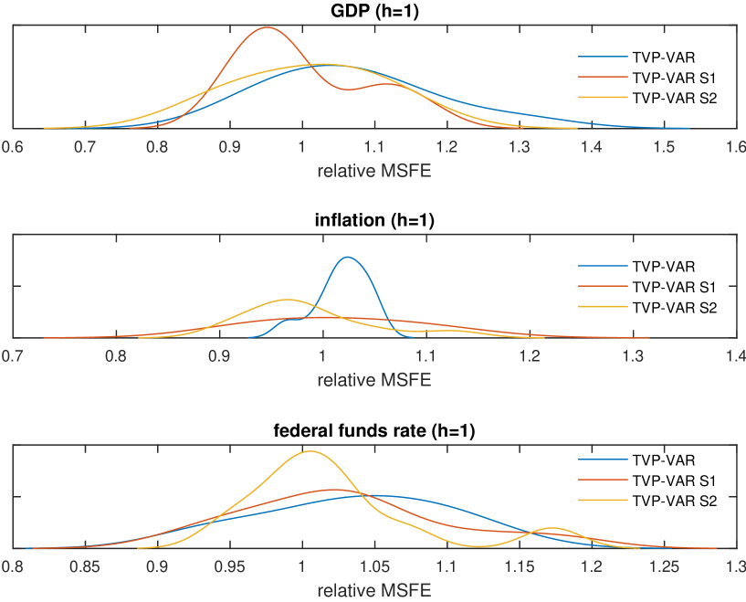
Figure A.1: Sampling distributions of the relative MSFEs (forecasting horizon: $h=1$ periods) - the benchmark is the TVP-VAR-DMA model in Koop and Korobilis (2013)

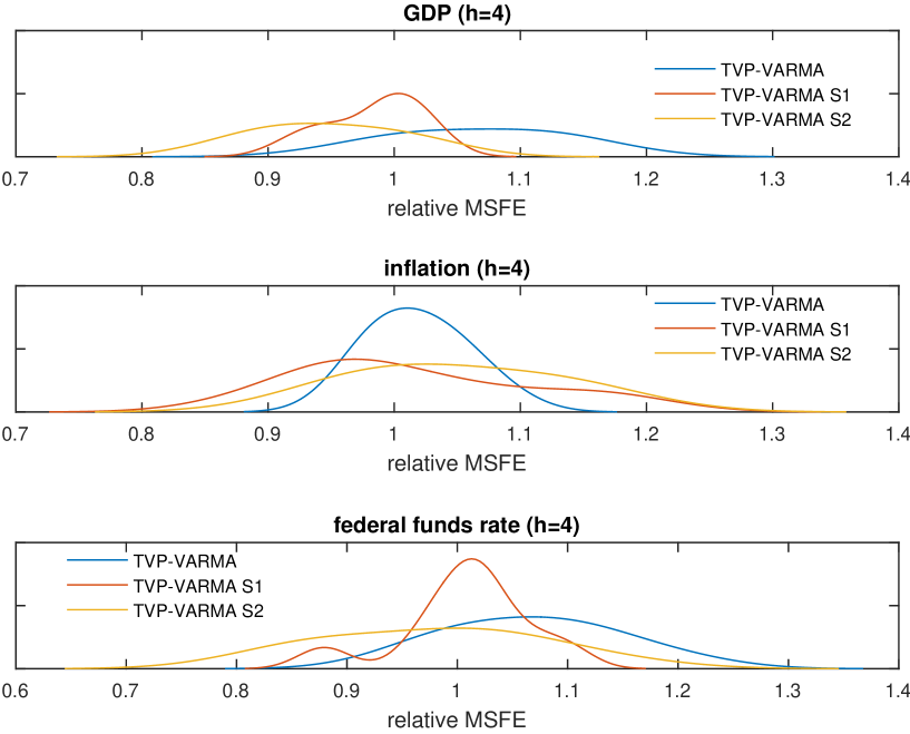
Figure A.2: Sampling distributions of the relative MSFEs (forecasting horizon: $h=4$ periods) - the benchmark is the TVP-VAR-DMA model in Koop and Korobilis (2013)

Appendix B Application to a VARMA using US data

In order to further illustrate the flexibility and the performance of our approach, we consider the estimation and the predictive ability of a VARMA model, applied to US macro data. Our exercise is based on Chan et al. (2016), who make a compelling case for the use of VARMAs, in light of their superior predictive ability (see also the theory in Lütkepohl and Poskitt, 1996). Yet, VARMAs, as well as suffering from well-known identification issues (see e.g. the recent contribution by Gouriéroux et al., 2019) are liable to overparameterisation, and therefore dimensionality, in this context, is a very important issue.
In this application, we do not consider time variation: the purpose of our analysis is only to show the computational advantages of our procedure. We follow Chan et al. (2016), using the same dataset. The data are quarterly US macroeconomic variables, ranging from 1959:Q1 to 2013:Q4. All data are first-differenced to obtain stationarity, as is customarily recommended in this type of analysis (see Carriero et al., 2015) - see Table B.1 for a list of variables employed. In order to ensure a meaningful comparison with Chan et al. (2016), we consider three models of increasing dimension, with $n=3,7$ and $12$. In particular, for the model with $n=3$ variables, we have used: Real GDP, CPI (All Items) and Effective Federal Funds Rate. For the case $n=7$, the variables are the ones in the previous model, plus: Average Hourly Earnings: Manufacturing, M2 Money Stock, Spot Oil Price (WTI), and S&P 500 Index. Finally, for the model with $n=12$, the additional variables are Real Personal Consumption, Housing Starts (total), Real GPDI, ISM PMI Composite Index and All Employees (Total nonfarm).

Table B.1: List of variables employed in Chan et al. (2016)

GDP	GDP	GDP
CPI (All Items)	CPI (All Items)	CPI (All Items)
Effective Fed Fund Rate	Effective Fed Fund Rate	Effective Fed Fund Rate
	Average Hourly Earnings (Manifacturing)	Average Hourly Earnings (Manifacturing)
	M2	M2
	Spot Oil Price (WTI)	Spot Oil Price (WTI)
	S&P500 Index	S&P500 Index
		Real Personal Consumption
		Housing Starts (total)
		Real GDPI
		ISM PMI Composite Index
		All Employees (total nonfarm)

From a methodological point of view, given the posterior $p\left(\theta\right)$, we employ the same resampling scheme as suggested in Girolami and Calderhead (2011); the algorithm is essentially the same as the one reported in Section 2.2.3. The only difference is the proposal density employed in GC-Step 2, which in the case of a fixed parameter VARMA is defined as

$$q\left(\widetilde{\theta}|\theta_{k}\right)\sim N\left(\theta_{k},\varepsilon^{2}G^{-1}\left(\theta_{k}\right)\right),$$ (B.1)

where $\varepsilon$ is chosen so as to pre-determine, roughly, the acceptance ratio in GC-Step 4 of the algorithm, setting it to around $25-30$. We do this using $600,000$ replications, with a burn-in period of $100,000$ replications.

In Table B.2, we compare models using the sum of the log predictive likelihood as a model selection criterion based on forecasting accuracy (see also an insightful contribution by Geweke and Amisano, 2014). As can be noted, our methodology yields results which, broadly speaking, are as good as the ones in Chan et al. (2016); a distinctive advantage is that our procedure is simpler and quicker to implement (CPU times are always below 1’ using mainframe). Similarly to Chan et al. (2016), we note that VARMA models seem to offer better predictive power; yet, remarkably, our VAR($4$) based on using the dimension reduction strategy denoted as S2 is at least as good (in fact, marginally better) than both our VARMA($4,4$), and the one in Chan et al. (2016). Interestingly, it can be noted that model averaging yields an even better result. This can be viewed as an indication that none of the models under consideration is correctly specified, which makes the case for model averaging.

Table B.2: Sum of log predictive likelihoods for various specifications

	$n=3$	$n=7$	$n=12$	$W$
Chan et al. (2016)
$VARMA(4,4)^{\left(a\right)}$	$-182.5$	$-401.9$	$-492.3$
$VARMA(4,4)^{\left(b\right)}$	$-188.1$	$-406.0$	$-504.2$
$VAR(4)$	$-187.1$	$-406.7$	$-496.9$
This paper
$VAR(4)$	$-187.1$	$-406.8$	$-496.9$	$0.24$
$VARMA(4,4)$	$-182.5$	$-401.9$	$-492.1$	$0.29$
$VAR(4)$ with $S1$	$-187.0$	$-406.7$	$-496.7$	$0.22$
$VAR(4)$ with $S2$	$-182.3$	$-401.7$	$-492.0$	$0.21$
Model average	$-179.4$	$-401.1$	$-490.0$	$0.32$

• The table contains the sums of the log predictive likelihood for various specifications - in panel “Chan et al. (2016)”, we consider various VARMA specifications using the methodology proposed in Chan et al. (2016) - the superscripts “^(a)”and “^(b)”refer to two different prior specifications; in panel “This paper”, we have considered various specifications based on our methodology.

• When using the two strategies S1 and S2 described in Section 2.2.2, $G$ has been selected by maximising the integrated likelihood as a selection criterion; in all cases, we this has led to the choice $G=3$.

• In the “Model average”row, we use a standard Bayesian model averaging, based on weights computed from the posterior model probabilities (details are available upon request); we have used $10,000$ sets of weights.

• The column denoted as $W$ contains the inefficiency factor of our MCMC - see e.g. Chib and Greenberg (1996) for a definition.

We have also run a complementary exercise, in which we estimate the three models (with $n=3,7$ and $12$ variables), and then consider the predictive likelihood for the variables that are common to the three specifications - that is, Real GDP, CPI (All Items) and Effective Federal Funds Rate. The results are presented in Table B.3, where it can be noted that the forecasting ability (slightly) improves as $n$ increases, reinforcing the case for large VARs. Especially when $n=12$ is considered, our approach to the estimation of VARMA($4,4$) delivers the best predictive ability - again, this result should be read in conjunction with the decidedly lower CPU time of our approach.

Table B.3: Sum of log predictive likelihoods - predictions of GDP, CPI and interest rates

	$n=3$	$n=7$	$n=12$
Chan et al. (2016)
$VARMA(4,4)^{\left(a\right)}$	$-182.5$	$-182.2$	$-181.1$
$VARMA(4,4)^{\left(b\right)}$	$-188.1$	$-185.4$	$-187.4$
$VAR(4)$	$-187.1$	$-187.2$	$-191.0$
This paper
$VAR(4)$	$-183.1$	$-184.2$	$-189.0$
$VARMA(4,4)$	$-180.5$	$-180.2$	$-180.0$

• The table contains the sum of the log predictive likelihoods based on the predictive densities of the first three variables (Real GDP, CPI and Interest rate). All other specifications are the same as in Table B.2.

• Note that we do not report the weighted average, since the posterior model probabilities favour only one model.

Finally, we point out that we have also carried out impulse response analysis; whilst we do not report results (which are available upon request), we found that impulse response functions behave in a very similar way to those in Figures 1 and 2 in Chan et al. (2016).

References

- Bańbura et al. (2010) Bańbura, M., D. Giannone, and L. Reichlin (2010). Large Bayesian vector auto regressions. Journal of Applied Econometrics 25(1), 71–92.
- Bassetti et al. (2014) Bassetti, F., R. Casarin, and F. Leisen (2014). Beta-product dependent Pitman–Yor processes for Bayesian inference. Journal of Econometrics 180(1), 49–72.
- Canova (1993) Canova, F. (1993). Modelling and forecasting exchange rates with a Bayesian time-varying coefficient model. Journal of Economic Dynamics and Control 17(1-2), 233–261.
- Cappé et al. (2009) Cappé, O., E. Moulines, and T. Rydén (2009). Inference in hidden Markov models. In Proceedings of EUSFLAT conference, pp. 14–16.
- Carriero et al. (2015) Carriero, A., T. E. Clark, and M. Marcellino (2015). Bayesian VARs: specification choices and forecast accuracy. Journal of Applied Econometrics 30(1), 46–73.
- Carriero et al. (2016) Carriero, A., T. E. Clark, and M. Marcellino (2016). Common drifting volatility in large Bayesian VARs. Journal of Business & Economic Statistics 34(3), 375–390.
- Carriero et al. (2019) Carriero, A., T. E. Clark, and M. Marcellino (2019). Large bayesian vector autoregressions with stochastic volatility and non-conjugate priors. Journal of Econometrics 212, 137–154.
- Chan et al. (2013) Chan, J. C., E. Eisenstat, et al. (2013). Gibbs samplers for VARMA and its extensions. Technical report, Australian National University, College of Business and Economics.
- Chan et al. (2016) Chan, J. C., E. Eisenstat, and G. Koop (2016). Large bayesian VARMAs. Journal of Econometrics 192(2), 374–390.
- Chen and Huang (2007) Chen, S. X. and T.-M. Huang (2007). Nonparametric estimation of copula functions for dependence modelling. Canadian Journal of Statistics 35(2), 265–282.
- Chib and Greenberg (1996) Chib, S. and E. Greenberg (1996). Markov chain monte carlo simulation methods in econometrics. Econometric Theory 12(3), 409–431.
- Clark (2011) Clark, T. E. (2011). Real-time density forecasts from bayesian vector autoregressions with stochastic volatility. Journal of Business & Economic Statistics 29(3), 327–341.
- Clark and Ravazzolo (2015) Clark, T. E. and F. Ravazzolo (2015). Macroeconomic forecasting performance under alternative specifications of time-varying volatility. Journal of Applied Econometrics 30(4), 551–575.
- Cogley and Sargent (2001) Cogley, T. and T. J. Sargent (2001). Evolving post-World War II US inflation dynamics. NBER macroeconomics annual 16, 331–373.
- Creal and Tsay (2015) Creal, D. D. and R. S. Tsay (2015). High dimensional dynamic stochastic copula models. Journal of Econometrics 189(2), 335–345.
- Di Lucca et al. (2013) Di Lucca, M. A., A. Guglielmi, P. Müller, and F. A. Quintana (2013). A simple class of Bayesian nonparametric autoregression models. Bayesian Analysis (Online) 8(1), 63.
- Doan et al. (1984) Doan, T., R. Litterman, and C. Sims (1984). Forecasting and conditional projection using realistic prior distributions. Econometric Reviews 3(1), 1–100.
- Geweke and Amisano (2014) Geweke, J. and G. Amisano (2014). Analysis of variance for Bayesian inference. Econometric Reviews 33(1-4), 270–288.
- Geweke and Keane (2007) Geweke, J. and M. Keane (2007). Smoothly mixing regressions. Journal of Econometrics 138(1), 252–290.
- Giannone et al. (2015) Giannone, D., M. Lenza, and G. E. Primiceri (2015). Prior selection for vector autoregressions. Review of Economics and Statistics 97(2), 436–451.
- Giannone and Reichlin (2006) Giannone, D. and L. Reichlin (2006). Does information help recovering structural shocks from past observations? Journal of the European Economic Association 4(2-3), 455–465.
- Girolami and Calderhead (2011) Girolami, M. and B. Calderhead (2011). Riemann manifold Langevin and Hamiltonian Monte Carlo methods. Journal of the Royal Statistical Society: Series B (Statistical Methodology) 73(2), 123–214.
- Gouriéroux et al. (2019) Gouriéroux, C., A. Monfort, and J.-P. Renne (2019). Identification and estimation in non-fundamental structural VARMA models. The Review of Economic Studies, to appear.
- Gruber and Czado (2015) Gruber, L. and C. Czado (2015). Sequential Bayesian model selection of regular vine copulas. Bayesian Analysis 10(4), 937–963.
- Gruber and Czado (2018) Gruber, L. F. and C. Czado (2018). Bayesian model selection of regular vine copulas. Bayesian Analysis 13(4), 1107–1131.
- Guhaniyogi and Dunson (2015) Guhaniyogi, R. and D. B. Dunson (2015). Bayesian compressed regression. Journal of the American Statistical Association 110(512), 1500–1514.
- Humphreys et al. (2015) Humphreys, D. A., P. M. Harris, M. Rodríguez-Higuero, F. A. Mubarak, D. Zhao, and K. Ojasalo (2015). Principal component compression method for covariance matrices used for uncertainty propagation. IEEE Transactions on Instrumentation and Measurement 64(2), 356–365.
- Ibragimov (2005) Ibragimov, R. (2005). Copula-based dependence characteriztions and modeling for time series. Harvard Institute of Economic Research Discussion Paper (2094).
- Jeffreys (1998) Jeffreys, H. (1998). The theory of probability. OUP Oxford.
- Kapetanios et al. (2019) Kapetanios, G., M. Marcellino, and F. Venditti (2019). Large time-varying parameter VARs: A non-parametric approach. Journal of Applied Econometrics, to appear.
- Kim et al. (1998) Kim, S., N. Shephard, and S. Chib (1998). Stochastic volatility: likelihood inference and comparison with ARCH models. The Review of Economic Studies 65(3), 361–393.
- Koop and Korobilis (2013) Koop, G. and D. Korobilis (2013). Large time-varying parameter VARs. Journal of Econometrics 177(2), 185–198.
- Koop et al. (2019) Koop, G., D. Korobilis, and D. Pettenuzzo (2019). Bayesian compressed vector autoregressions. Journal of Econometrics 210(1), 135–154.
- Korobilis and Pettenuzzo (2019) Korobilis, D. and D. Pettenuzzo (2019). Adaptive hierarchical priors for high-dimensional vector autoregressions. Journal of Econometrics 212, 241–271.
- Litterman (1986) Litterman, R. B. (1986). Forecasting with Bayesian vector autoregressions: five years of experience. Journal of Business & Economic Statistics 4(1), 25–38.
- Lütkepohl (2005) Lütkepohl, H. (2005). New introduction to multiple time series analysis. Springer Science & Business Media.
- Lütkepohl and Poskitt (1996) Lütkepohl, H. and D. S. Poskitt (1996). Specification of echelon-form VARMA models. Journal of Business & Economic Statistics 14(1), 69–79.
- Nelsen (2007) Nelsen, R. B. (2007). An introduction to copulas. Springer Science & Business Media.
- Nemeth et al. (2016) Nemeth, C., C. Sherlock, and P. Fearnhead (2016). Particle Metropolis-adjusted Langevin algorithms. Biometrika 103(3), 701–717.
- Nieto-Barajas et al. (2012) Nieto-Barajas, L. E., P. Müller, Y. Ji, Y. Lu, and G. B. Mills (2012). A time-series DDP for functional proteomics profiles. Biometrics 68(3), 859–868.
- Nieto-Barajas and Quintana (2016) Nieto-Barajas, L. E. and F. A. Quintana (2016). A Bayesian non-parametric dynamic AR model for multiple time series analysis. Journal of Time Series Analysis 37(5), 675–689.
- Primiceri (2005) Primiceri, G. E. (2005). Time varying structural vector autoregressions and monetary policy. The Review of Economic Studies 72(3), 821–852.
- Roberts and Rosenthal (1998) Roberts, G. O. and J. S. Rosenthal (1998). Optimal scaling of discrete approximations to Langevin diffusions. Journal of the Royal Statistical Society: Series B (Statistical Methodology) 60(1), 255–268.
- Rodriguez and ter Horst (2008) Rodriguez, A. and E. ter Horst (2008). Bayesian dynamic density estimation. Bayesian Analysis 3(2), 339–365.
- Scaillet and Fermanian (2003) Scaillet, O. and J.-D. Fermanian (2003). Nonparametric estimation of copulas for time series. Journal of Risk (5), 25–54.
- Sims (1980) Sims, C. A. (1980). Macroeconomics and reality. Econometrica 48, 1–48.
- Sims (1993) Sims, C. A. (1993). A nine-variable probabilistic macroeconomic forecasting model. In Business Cycles, Indicators and Forecasting, pp. 179–212. University of Chicago Press.
- Sklar (1996) Sklar, A. (1996). Random variables, distribution functions, and copulas: a personal look backward and forward. Lecture notes-monograph series, 1–14.
- Sklar (1959) Sklar, M. (1959). Fonctions de repartition an dimensions et leurs marges. Publ. Inst. Statist. Univ. Paris 8, 229–231.
- Stock and Watson (1996) Stock, J. H. and M. W. Watson (1996). Evidence on structural instability in macroeconomic time series relations. Journal of Business & Economic Statistics 14(1), 11–30.
- Taddy (2010) Taddy, M. A. (2010). Autoregressive mixture models for dynamic spatial Poisson processes: Application to tracking intensity of violent crime. Journal of the American Statistical Association 105(492), 1403–1417.
- Tewari et al. (2011) Tewari, A., M. J. Giering, and A. Raghunathan (2011). Parametric characterization of multimodal distributions with non-gaussian modes. In 2011 IEEE 11th International Conference on Data Mining Workshops, pp. 286–292. IEEE.
- Tsionas et al. (2019) Tsionas, M., M. Izzeldin, and L. Trapani (2019). Copula-based Bayesian estimation of large multivariate stochastic volatility models. Technical report.
- Uhlig (1997) Uhlig, H. (1997). Bayesian vector autoregressions with stochastic volatility. Econometrica 65, 59–74.
- Villani et al. (2009) Villani, M., R. Kohn, and P. Giordani (2009). Regression density estimation using smooth adaptive Gaussian mixtures. Journal of Econometrics 153(2), 155–173.
- Watson (1994) Watson, M. W. (1994). Vector autoregressions and cointegration. Handbook of Econometrics 4, 2843–2915.