Tha3aroon at NSURL-2019 Task 8: Semantic Question Similarity in Arabic

Abstract

In this paper, we describe our team’s effort on the semantic text question similarity task of NSURL 2019. Our top performing system utilizes several innovative data augmentation techniques to enlarge the training data. Then, it takes ELMo pre-trained contextual embeddings of the data and feeds them into an ON-LSTM network with self-attention. This results in sequence representation vectors that are used to predict the relation between the question pairs. The model is ranked in the 1st place with 96.499 F1-score (same as the second place F1-score) and the 2nd place with 94.848 F1-score (differs by 1.076 F1-score from the first place) on the public and private leaderboards, respectively.

1 Introduction

Semantic Text Similarity (STS) problems are both real-life and challenging. For example, in the paraphrase identification task, STS is used to predict if one sentence is a paraphrase of the other or not Madnani et al. (2012); He et al. (2015); AL-Smadi et al. (2017). Also, in answer sentence selection task, it is utilized to determine the relevance between question-answer pairs and rank the answers sentences from the most relevant to the least. This idea can also be applied to search engines in order to find documents relevant to a query Yang et al. (2015); Tan et al. (2018); Yang et al. (2019).

A new task has been proposed by Mawdoo3 company with a new dataset provided by their data annotation team for Semantic Question Similarity (SQS) for the Arabic language Schwab et al. (2017); Mahmoud et al. (2017); Alian and Awajan (2018). SQS is a variant of STS, which aims to compare a pair of questions and determine whether they have the same meaning or not. The SQS in Arabic task is one of the shared tasks of the Workshop on NLP Solutions for Under Resourced Languages (NSURL 2019) and it consists of 12K questions pairs Seelawi et al. (2019).

In this paper, we describe our team’s efforts to tackle this task. After preprocessing the data, we use four data augmentation steps to enlarge the training data to about four times the size of the original training data. We then build a neural network model with four components. The model uses ELMo (which stands for Embeddings from Language Models) Peters et al. (2018) pre-trained contextual embeddings as an input and builds sequence representation vectors that are used to predict the relation between the question pairs. The task is hosted on Kaggle platform and our model is ranked in the first place with 96.499 F1-score (same as the second place F1-score) and in the second place with 94.848 F1-score (differs by 1.076 F1-score from the first place) on the public and private leaderboards, respectively.

The rest of this paper is organized as follows. In Section 2, we describe our methodology, including data preprocessing, data augmentation, and model structure, while in Section 3, we present our experimental results and discuss some insights from our model. Finally, the paper is concluded in Section 4.

2 Methodology

In this section, we present a detailed description of our model. We start by discussing the preprecessing steps we take before going into the details of the first novel aspect of our work, which is the data augmentation techniques. We then discuss the neural network model starting from the input all the way to the decision step. The implementation is available on a public repository.

2.1 Data Preprocessing

In this work, we only consider one preprocessing step, which is to separate the punctuation marks shown in Figure 1 from the letters. For example, if the question was: ‘‘مرحبا، كيف الحال؟>’’, then it will be processed as follows: ‘‘مرحبا ، كيف الحال ؟>’’. This is done to preserve as much information as possible in the questions while keeping the words clear of punctuations.

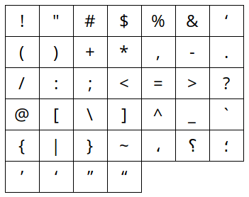
Figure 1: Punctuation marks considered in the preprocessing step

2.2 Data Augmentation

The training data contains 11,997 question pairs: 5,397 labeled as 1 (i.e., similar) and 6,600 labeled as 0 (i.e., not similar). To obtain a larger dataset, we augment the data using the following rules.

Suppose we have questions A, B and C

• Positive Transitive:

  If A is similar to B, and B is similar to C, then A is similar to C.

• Negative Transitive:

  If A is similar to B, and B is NOT similar to C, then A is NOT similar to C.

  Note: The previous two rules generates 5,490 extra examples (bringing the total up to 17,487).

• Symmetric:

  If A is similar to B then B is similar to A, and if A is not similar to B then B is not similar to A.

  Note: This rule doubles the number of examples to 34,974 in total.

• Reflexive:

  By definition, a question A is similar to itself.

  Note: This rule generates 10,540 extra positive examples (45,514 total) which helps balancing the number of positive and negative examples.

After the augmentation process, the training data contains 45,514 examples (23,082 positive examples and 22,432 negative ones). Figure 2 shows the growth of the training dataset after each data augmentation step.

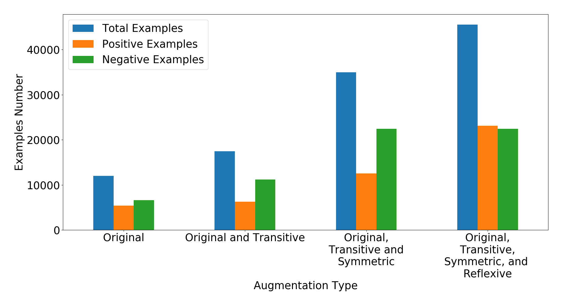
Figure 2: Number of examples per data augmentation step

2.3 Model Structure

We now discuss our model structure, which is shown in Figure 3. As the figure shows, the model structure can be divided into the following components/layers: input layer, sequence representation extraction layer, merging layer and decision layer. The following subsections explain each layer/component in details.

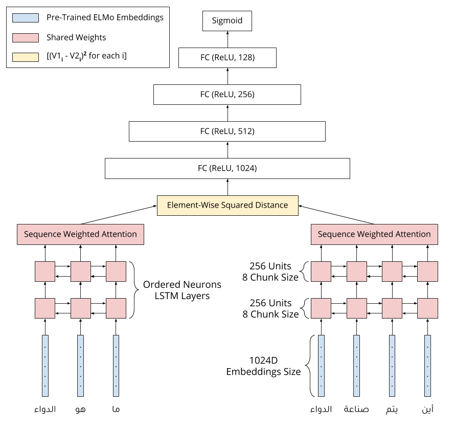
Figure 3: Model Structure

2.3.1 Input

To build meaningful representations for the input sequences, we use the Arabic ELMo pre-trained model to extract contextual words embeddings with size 1024 and feed them as input to our model. The representations extracted from the ELMo model are the averaged sum of word encoder and both first and second Long Short-Term Memory (LSTM) hidden layers. These representations are affected by the context in which they appear Cheng et al. (2015); Peters et al. (2018); Smith (2019). For example, the word ‘‘ذهب>’’ will have different embedding vectors related to the following two sentences as they have different meanings (‘gold’ in the first sentence and ‘went’ in the second one):

ذهب علي كثير >
Translation: Ali has a lot of gold.
ذهب علي بعيدا >
Translation: Ali went away.

2.3.2 Sequence Representation Extractor

This component takes the ELMo embeddings related to each word in the question as an input and feeds them into two a special kind of bidirectional LSTM layers called Ordered Neurons LSTM (ON-LSTM) introduced in Shen et al. (2018) with 256 hidden units, 20% dropout rate, and 8 as the chunk size for each of them. Then, it applies sequence weighted attention proposed by Felbo et al. (2017) on the outputs of the second ON-LSTM layer to get the final question representation. This component uses the same weights to compute representations for each question in the pair. The details of this component are as follows Shen et al. (2018).

Since NLP data are structured in a hierarchical manner, the authors of ON-LSTM Shen et al. (2018) proposed a new form of update and activation functions (in order to enforce a bias towards structuring a hierarchy of the data) to the standard LSTM model reported below:

$$f_{t} =\sigma_{g}(W_{f}x_{t}+U_{f}h_{t-1}+b_{f})$$ (1)

$$i_{t} =\sigma_{g}(W_{i}x_{t}+U_{i}h_{t-1}+b_{i})$$ (2)

$$o_{t} =\sigma_{g}(W_{o}x_{t}+U_{o}h_{t-1}+b_{o})$$ (3)

$$\hat{c_{t}} =\tanh(W_{c}x_{t}+U_{c}h_{t-1}+b_{c})$$ (4)

$$h_{t} =o_{t}\circ\tanh(c_{t})$$ (5)

The newly proposed activation function is $cumax=cumsum(softmax(x))$, where $cumsum$ denotes the cumulative sum function. Among the desired properties of this function is to control the updates on the memory cell such that the higher ranking neurons get updated less frequently (storing long-term and global information) compared to the lower ranking neurons, which are updated more frequently (storing short-term and local information). This makes the neurons updates dependent on each other in contrast to the updates on the standard LSTM neurons.

The following equations define the new master input and forget gates and the new memory cell update function based on the new activation function:

$$\tilde{f_{t}} =cumax(W_{\tilde{f}}x_{t}+U_{\tilde{f}}h_{t-1}+b_{\tilde{f}})$$ (6)

$$\tilde{i_{t}} =1-cumax(W_{\tilde{i}}x_{t}+U_{\tilde{i}}h_{t-1}+b_{\tilde{i}})$$ (7)

$$w_{t} =\tilde{f_{t}}\circ\tilde{i_{t}}$$ (8)

$$\hat{f_{t}} =f_{t}\circ w_{t}+(\tilde{f_{t}}-w_{t})$$ (9)

$$\hat{i_{t}} =i_{t}\circ w_{t}+(\tilde{i_{t}}-w_{t})$$ (10)

$$c_{t} =\hat{f_{t}}\circ c_{t-1}+\hat{i_{t}}\circ\hat{c_{t}}$$ (11)

The attention mechanism (inspired by Bahdanau et al. (2014); Yang et al. (2016)) allows the model to learn to decide the importance of each word and build the final question representation vector based on important words only, while tuning out less important words. With a single parameter, $w_{a}$, the attention mechanism can be described as follows:

$$e_{t} =h_{t}w_{a}$$ (12)

$$a_{t} =\frac{exp(e_{t})}{\sum_{i=1}^{T}exp(e_{i})}$$ (13)

$$v =\sum_{i=1}^{T}a_{i}h_{i}$$ (14)

The weight matrix $w_{a}$ is the only new trainable parameter which learns the attention mechanism over the outputs of the second ON-LSTM layer. To calculate the importance scores, $a_{t}$, for each time step, it first multiplies each time step output, $h_{t}$, by the weight matrix, $w_{a}$, and normalizes the results using a Softmax function. Finally, the final sequence representation, $v$, is the weighted sum over all ON-LSTM outputs using the importance scores calculated earlier as weights.

2.3.3 Merging Technique

After extracting the representations related to each question, we merge them using pairwise squared distance function applied to the representation vectors of the two questions in each question pair. More formally, if $V1$ and $V2$ are these representation vectors, then, the merged representation vector $Vm$ can be expressed as follows:

$$Vm=\begin{bmatrix}(V1_{1}-V2_{1})^{2}\\ (V1_{2}-V2_{2})^{2}\\ \vdots\\ (V1_{512}-V2_{512})^{2}\end{bmatrix}$$ (15)

This component allows for the Symmetric augmentation step (Section 2.2) to enhance the results, since the $(A,B)$ examples are computationally different (in the back propagation step) from the $(B,A)$ examples.

2.3.4 Deep Neural Network

The final component is a deep neural network that consists of four fully-connected layers with 1024, 512, 256, and 128 units using ReLU activation function and 20% dropout rate applied to each layer. This network takes the merged representation vector, $Vm$, as an input and predicts the label using a Sigmoid function as an output.

3 Experiments and Results

In this section, we start by discussing our experimental setup. We then discuss all experiments conducted and provide detailed analysis of their results.

3.1 Experimental Setup

All experiments discussed in this work have been done on the Google Colab Carneiro et al. (2018) environment using Tesla T4 GPU accelerator with the following hyperparameters:

• Optimizer: Adam

• Learning Rate: 0.001

• Loss Function: Binary Cross Entropy

• Batch Size: 256

• Number of Epochs: 100

The experiments are divided into two sets. The first set aims to explore the effect of the Recurrent Neural Network (RNN) cell type, while the second set aims to explore the effect of the data augmentation techniques mentioned in Section 2.2.

For each experiment, five models are trained and the following results are reported:

• Minimum F1 score gained on the test set.

• Maximum F1 score gained on the test set.

• Average F1 score gained from the five trained models.

• Majority Voting F1 score gained by ensembling the five trained models.

3.2 Effect of RNN Cell Type

Table 1: Model size and training time for each RNN cell type

RNN Cell	#Params	Training Time
GRU	4,363K	55.2s/epoch - 1.53 hours
LSTM	5,413K	58.2s/epoch - 1.61 hours
ON-LSTM (Chunk: 4)	5,938K	74.2s/epoch - 2.06 hours
ON-LSTM (Chunk: 8)	5,675K	74.4s/epoch - 2.06 hours

Table 2: Model F1-score using different RNN cell types

Leaderboard	RNN Cell	Min	Max	Avg	Vote
Public	GRU	94.075	94.793	94.613	95.242
	LSTM	94.614	95.152	94.901	95.062
	ON-LSTM (Chunk: 4)	94.524	95.601	95.242	96.140
	ON-LSTM (Chunk: 8)	95.601	95.780	95.691	96.499
Private	GRU	93.271	94.194	93.855	94.579
	LSTM	93.925	94.271	94.040	94.117
	ON-LSTM (Chunk: 4)	93.810	94.425	94.224	94.732
	ON-LSTM (Chunk: 8)	94.002	94.463	94.309	94.848

In this experiments set, we use the same structure described in Section 2.3 while changing the RNN cell type only. We use all 45,514 examples from the augmented dataset in the training process. The tested RNN cells are: Gated Recurrent Unit (GRU) Cho et al. (2014), LSTM Hochreiter and Schmidhuber (1997) and ON-LSTM Shen et al. (2018). The latter one is tested using two chunk sizes, 4 and 8, in order to explore the effect of chunk size on the training process and the size of the model. Table 1 shows the model size in terms of trainable parameters and the training time for each RNN cell type, while Table 2 shows the F1-scores of the model using different RNN cells. Best results are shown in bold. The tables show that while GRU cells are the most efficient, the ON-LSTM cells (with chunk size 8) are the most effective (in terms of all considered measures).

3.3 Effect of Data Augmentation

In this experiments set, we use the RNN cell type that gives the best results in Section 3.2 (ON-LSTM with chunk size 8) and the same model structure described in Section 2.3 to explore the effect of data augmentation steps mentioned in Section 2.2.

The data augmentation steps have an effect on two factors, the training time and the accuracy measurement (F1-score). Table 3 shows the average training time over five runs for each data augmentation step. Moreover, Table 4 shows the F1-scores of the trained model using different data augmentation types, best results shown in bold.

Table 3: Model training time for each data augmentation step: O, T, S, and R, which stand for Original, Transitive, Symmetric, and Reflexive, respectively

Data Augmentation	Examples Number	Training Time
O	11,997	20.0s/epoch - 0.55 hours
O+T	17,487	29.4s/epoch - 0.81 hours
O+T+S	34,974	57.0s/epoch - 1.58 hours
O+T+S+R	45,514	74.4s/epoch - 2.06 hours

Table 4: Model F1-score using different data augmentation types: O, T, S, and R, which stand for Original, Transitive, Symmetric, and Reflexive respectively

Leaderboard	Data Aug.	Min	Max	Avg	Vote
Public	O	93.626	94.703	94.200	94.973
	O+T	93.177	94.434	93.877	94.793
	O+T+S	94.344	94.793	94.631	95.421
	O+T+S+R	95.601	95.780	95.691	96.499
Private	O	93.425	93.810	93.632	94.655
	O+T	92.464	93.771	93.232	94.156
	O+T+S	93.579	94.002	93.763	94.655
	O+T+S+R	94.002	94.463	94.309	94.848

The tables show that each augmentation step affects the model’s efficiency negatively. This is expected since each step incrementally increases the size of the dataset. On the other hand, not each increment step has a positive effect on the model’s effectiveness. Such trends are worth exploring in a more exhaustive study. Finally, it is worth mentioning that the last experiments in both experiment sets are the same. So, they both have the same results.

3.4 Other Attempts

We test several other techniques to explore how they might affect our model. For example, using pre-trained FastText Bojanowski et al. (2017) embeddings as an input to our model yields worse F1-score on both public and private leaderboards with 94.254 and 93.118, respectively, compared with the ELMo contextual embeddings model. In another experiment, we use the thought vector outputted from the second ON-LSTM layer as input for the decision component. However, the sequence weighted attention gives better results by about 1 point of the F1-score. Moreover, an attempt to overcome the weakness of the Arabic ELMo model is done by translating the data to English using Google Translate and treating the problem as an English SQS problem instead, but the results are much worse with 88.868 and 87.504 F1-scores on public and private leaderboards, respectively. This is probably because a lot of information is lost during the translation process.

3.5 Discussion

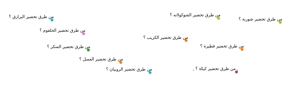
Figure 4: Representations extracted from sequence weighted attention layer for questions of the form: How to prepare ‘something’?

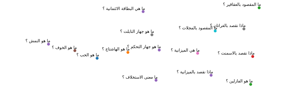
Figure 5: Representations extracted from sequence weighted attention layer for questions of the form: What is the definition of ‘something’?

This section briefly analyzes the questions representations learnt by our model. With the sequence weighted attention layer, the model reduces all the information about the sequence extracted using the ON-LSTMs down to a 512 fixed-size vector. By extracting these vectors from our best model and plotting them on a 2D plane using t-SNE Maaten and Hinton (2008) dimensionality reduction algorithm, we notice some very useful observations. For example, the model learns to map questions that ask about the same thing to have nearby representations in the vector space such as the questions in Figure 4 with the form: ‘‘How to prepare ‘something’?’’. The same thing goes for the questions in Figure 5 with the form: ‘‘What is the definition of ‘something’?’’. In a similar manner, in Figure 6, the questions ask about different types of languages like ‘‘What is the formal language in Portugal?’’ and ‘‘What is PHP language?’’ are close, as well as, the questions in Figure 7 that ask about places like ‘‘Where is Sweden?’’, ‘‘Where is the Karak area in Jordan?’’, and ‘‘Where is the Kremlin Castle?’’.

To further illustrate the usefulness of the sequence weighted attention layer, Figure 8 shows that the attention layer learns to focus more on the key words in the questions that would determine what the question is actually asking about. This allows the model to make better decisions for whether the the questions are similar or not, even if the questions have similar words but ask about different things. The first and second questions in Figure 8 ask about ‘‘What is the general manager?’’. So, the attention layer focuses on ‘‘the general manager’’ which is ‘‘المدير العام>’’. However, in the third and fourth questions, one asks ‘‘What is the most beautiful thing that is said about death?’’ and the other ones asks ‘‘What is death?’’, although both questions are related to ‘‘death’’ which is ‘‘الموت>’’ but the attention layer distinguishes them as not similar, where in the former one, the focus is concentrated by order on the words ‘‘قيل>’’, ‘‘أجمل>’’ and ‘‘بالموت>’’ (‘‘said’’, ‘‘most beautiful’’ and ‘‘death’’), while the latter one focuses mostly on ‘‘الموت>’’ (‘‘death’’).

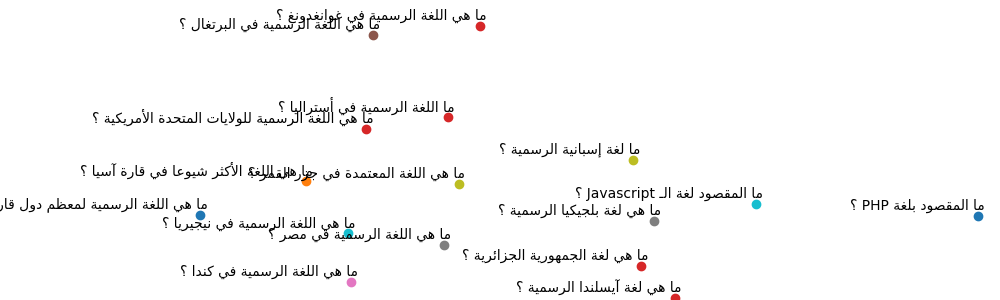
Figure 6: Representations extracted from sequence weighted attention layer for questions that ask about different language types

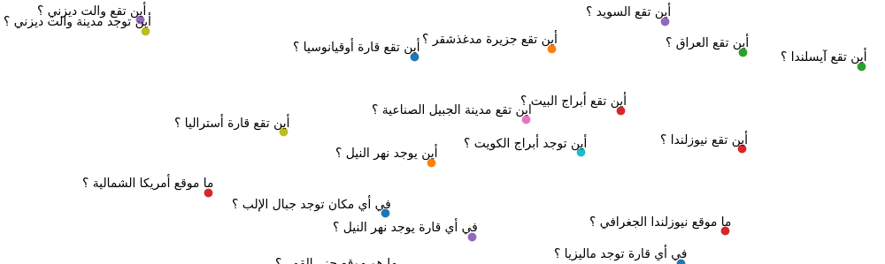
Figure 7: Representations extracted from sequence weighted attention layer for questions that ask about different places

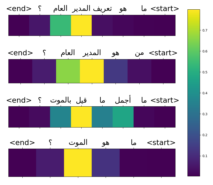
Figure 8: Weights per word from sequence weighted attention layer on four different examples

4 Conclusion

In this paper, we described our team’s effort on the semantic text question similarity task of NSURL 2019. Our top performing system utilizes several innovative data augmentation techniques to enlarge the training data. Then, it takes ELMo pre-trained contextual embeddings as an input and builds sequence representation vectors that are used to predict the relation between the question pairs. The model was ranked in the 1st place with 96.499 F1-score (same as the second place F1-score) and the 2nd place with 94.848 F1-score (differs by 1.076 F1-score from the first place) on the public and private leaderboards, respectively.

References

- AL-Smadi et al. (2017) Mohammad AL-Smadi, Zain Jaradat, Mahmoud Al-Ayyoub, and Yaser Jararweh. 2017. Paraphrase identification and semantic text similarity analysis in arabic news tweets using lexical, syntactic, and semantic features. Information Processing & Management, 53(3):640--652.
- Alian and Awajan (2018) Marwah Alian and Arafat Awajan. 2018. Arabic semantic similarity approaches-review. In 2018 International Arab Conference on Information Technology (ACIT), pages 1--6. IEEE.
- Bahdanau et al. (2014) Dzmitry Bahdanau, Kyunghyun Cho, and Yoshua Bengio. 2014. Neural machine translation by jointly learning to align and translate. arXiv preprint arXiv:1409.0473.
- Bojanowski et al. (2017) Piotr Bojanowski, Edouard Grave, Armand Joulin, and Tomas Mikolov. 2017. Enriching word vectors with subword information. Transactions of the Association for Computational Linguistics, 5:135--146.
- Carneiro et al. (2018) Tiago Carneiro, Raul Victor Medeiros Da Nóbrega, Thiago Nepomuceno, Gui-Bin Bian, Victor Hugo C De Albuquerque, and Pedro Pedrosa Reboucas Filho. 2018. Performance analysis of google colaboratory as a tool for accelerating deep learning applications. IEEE Access, 6:61677--61685.
- Cheng et al. (2015) Jianpeng Cheng, Zhongyuan Wang, Ji-Rong Wen, Jun Yan, and Zheng Chen. 2015. Contextual text understanding in distributional semantic space. In Proceedings of the 24th ACM International on Conference on Information and Knowledge Management, pages 133--142. ACM.
- Cho et al. (2014) Kyunghyun Cho, Bart Van Merriënboer, Caglar Gulcehre, Dzmitry Bahdanau, Fethi Bougares, Holger Schwenk, and Yoshua Bengio. 2014. Learning phrase representations using rnn encoder-decoder for statistical machine translation. arXiv preprint arXiv:1406.1078.
- Felbo et al. (2017) Bjarke Felbo, Alan Mislove, Anders Søgaard, Iyad Rahwan, and Sune Lehmann. 2017. Using millions of emoji occurrences to learn any-domain representations for detecting sentiment, emotion and sarcasm. arXiv preprint arXiv:1708.00524.
- He et al. (2015) Hua He, Kevin Gimpel, and Jimmy Lin. 2015. Multi-perspective sentence similarity modeling with convolutional neural networks. In Proceedings of the 2015 Conference on Empirical Methods in Natural Language Processing, pages 1576--1586.
- Hochreiter and Schmidhuber (1997) Sepp Hochreiter and Jürgen Schmidhuber. 1997. Long short-term memory. Neural computation, 9(8):1735--1780.
- Maaten and Hinton (2008) Laurens van der Maaten and Geoffrey Hinton. 2008. Visualizing data using t-sne. Journal of machine learning research, 9(Nov):2579--2605.
- Madnani et al. (2012) Nitin Madnani, Joel Tetreault, and Martin Chodorow. 2012. Re-examining machine translation metrics for paraphrase identification. In Proceedings of the 2012 Conference of the North American Chapter of the Association for Computational Linguistics: Human Language Technologies, pages 182--190. Association for Computational Linguistics.
- Mahmoud et al. (2017) Adnen Mahmoud, Ahmed Zrigui, and Mounir Zrigui. 2017. A text semantic similarity approach for arabic paraphrase detection. In International Conference on Computational Linguistics and Intelligent Text Processing, pages 338--349. Springer.
- Peters et al. (2018) Matthew E Peters, Mark Neumann, Mohit Iyyer, Matt Gardner, Christopher Clark, Kenton Lee, and Luke Zettlemoyer. 2018. Deep contextualized word representations. arXiv preprint arXiv:1802.05365.
- Schwab et al. (2017) Didier Schwab et al. 2017. Semantic similarity of arabic sentences with word embeddings.
- Seelawi et al. (2019) Haitham Seelawi, Ahmad Mustafa, Hesham Al-Bataineh, Wael Farhan, and Hussein T. Al-Natsheh. 2019. NSURL-2019 task 8: Semantic question similarity in arabic. In Proceedings of the first International Workshop on NLP Solutions for Under Resourced Languages, NSURL ’19, Trento, Italy.
- Shen et al. (2018) Yikang Shen, Shawn Tan, Alessandro Sordoni, and Aaron Courville. 2018. Ordered neurons: Integrating tree structures into recurrent neural networks. arXiv preprint arXiv:1810.09536.
- Smith (2019) Noah A Smith. 2019. Contextual word representations: A contextual introduction. arXiv preprint arXiv:1902.06006.
- Tan et al. (2018) Chuanqi Tan, Furu Wei, Wenhui Wang, Weifeng Lv, and Ming Zhou. 2018. Multiway attention networks for modeling sentence pairs. In IJCAI, pages 4411--4417.
- Yang et al. (2015) Yi Yang, Wen-tau Yih, and Christopher Meek. 2015. Wikiqa: A challenge dataset for open-domain question answering. In Proceedings of the 2015 Conference on Empirical Methods in Natural Language Processing, pages 2013--2018.
- Yang et al. (2019) Zhilin Yang, Zihang Dai, Yiming Yang, Jaime Carbonell, Ruslan Salakhutdinov, and Quoc V Le. 2019. Xlnet: Generalized autoregressive pretraining for language understanding. arXiv preprint arXiv:1906.08237.
- Yang et al. (2016) Zichao Yang, Diyi Yang, Chris Dyer, Xiaodong He, Alex Smola, and Eduard Hovy. 2016. Hierarchical attention networks for document classification. In Proceedings of the 2016 conference of the North American chapter of the association for computational linguistics: human language technologies, pages 1480--1489.