Non-linear damping of superimposed primordial oscillations on the matter power spectrum in galaxy surveys

Abstract

Galaxy surveys are an important probe for superimposed oscillations on the primordial power spectrum of curvature perturbations, which are predicted in several theoretical models of inflation and its alternatives. In order to exploit the full cosmological information in galaxy surveys it is necessary to study the matter power spectrum to fully non-linear scales. We therefore study the non-linear clustering in models with superimposed linear and logarithmic oscillations to the primordial power spectrum by running high-resolution dark-matter-only N-body simulations. We fit a Gaussian envelope for the non-linear damping of superimposed oscillations in the matter power spectrum to the results of the N-body simulations for $k\lesssim 0.6\ h/$Mpc at $0\leq z\leq 5$ with an accuracy below the percent. We finally use this fitting formula to forecast the capabilities of future galaxy surveys, such as Euclid and Subaru, to probe primordial oscillation down to non-linear scales alone and in combination with the information contained in CMB anisotropies.

1 Introduction

The study of departures from a simple power-law in the primordial power spectrum (PPS) of curvature perturbations has been fueled by theoretical advances and observational progress over many years (see Ref. [1] for a review).

From a theoretical perspective, departures from a simple power-law can be a signature of the breakdown of any of the assumptions behind standard single field slow-roll inflation with Bunch-Davies initial conditions for quantum fluctuations [2, 3, 4, 5, 6]. In the analogy in which primordial fluctuations can be seen as a cosmological collider for the physics of the early Universe [7, 8], these features could help in discriminating between inflation and alternative scenarios, or could provide hints for inflaton dynamics beyond slow-roll, and new heavy particles.

From the observational side, departures from a simple power-law in the PPS are of extreme interest, despite the tighter and tighter constraints on their size due to the increasing precision of cosmological observations. Well motivated theoretical models with features in the PPS have led to an improvement in the fit to cosmic microwave background (CMB) anisotropies data with respect to the simplest power-law spectrum since the WMAP first year data [9] to the final Planck legacy data release [10]. However, these improvements in the fit come at the expense of having extra parameters and these models have not been preferred over the simplest power-law spectrum at a statistically significant level so far, see e.g. [10].

Next generation of cosmological observations will help in explaining whether the hints for departures from a power-law spectrum for primordial fluctuations have a physical origin or are a mere statistical fluctuation. In particular, large-scale structure (LSS) surveys are very promising [11, 12, 13, 14, 15, 16, 17, 18, 19, 20, 21, 22, 23] since they can probe the PPS to smaller scales and can increase the range of scales which are independently scanned by CMB anisotropy measurements. It has been already quantified how future LSS surveys could significantly improve current constraints on theoretical models with features in the PPS by just using linear scales, i.e. $k\lesssim 0.1\ h/$Mpc [12, 15, 16, 21]. On the other hand, non-linear effects are important on most of the scales which are probed by LSS surveys and for these models are not accurately described by Halofit. Therefore, the study of non-linear dynamic is required to have full access to the information for primordial features contained in the dark matter (DM) power spectrum measurements as already studied in Refs. [24, 25, 26].

In this paper, we study two templates for the PPS which include undamped oscillations at small scales and therefore need the understanding of the non-linear gravitational instability at the scales of interest for galaxy surveys. Among the several models of primordial features, we choose the case of undamped linear or logarithmic oscillations superimposed on all the scales of interest to a PPS described by a power-law [27, 28, 29, 30, 32, 31, 33, 34, 35]: these are the theoretical models which lead to the largest improvement in the fit of CMB anisotropies and which need the understanding of non-linear clustering on scales $k\gtrsim 0.1\ h/$Mpc, given the presence of oscillations on all the scales. With these linear and logarithmic oscillations superimposed to the PPS we run a set of high-resolution DM-only cosmological simulations with 1,024³ DM particles in a comoving box with side length of 1,024 Mpc$/h$ (see [20] for N-body simulations with different type of primordial features). We then develop a fitting function calibrated against a set of N-body simulations with features in the PPS, following the approach previously used in Halofit [36, 37] or HM-Code [38, 39] for $\Lambda$CDM and some of its extensions.

The paper is organized as follows. We begin in Sec. 2 introducing the two templates for oscillatory features that we study. In Sec. 3.1, we describe the simulations. In Sec. 3.2, we use a Gaussian envelope for the non-linear damping and we calibrate it against the N-body simulations; we also compare our findings with the leading-order theoretical predictions for the damping from Refs. [25, 26]. We discuss in Sec. 4 the damping of the baryon acoustic oscillations (BAO) features versus the damping of the primordial linear oscillations. We run a series of forecasts in Sec. 5 with galaxy clustering up to $k_{\rm max}=0.6\ h/$Mpc in combination with CMB for a Euclid-like experiment and Subaru Prime Focus Spectrograph (PFS), and we discuss the results in Sec. 6. Sec. 7 contains our conclusions.

2 Superimposed oscillations on the primordial power spectrum

The type of superimposed oscillatory features on the PPS which we study in this paper are predicted in several well motivated theoretical models. These features can be generated by an oscillatory signal in time in the inflationary field potential or in the internal field space with a frequency larger than the Hubble parameter $H$ able to resonate with the curvature modes inside the horizon [27]. They can be realized in many contexts as in axion inflation [28], small-field models such as brane inflation [29], large-field models in string theory such as axion monodromy [30], or as oscillations of massive fields [32, 31]. Superimposed oscillations on the PPS are also generated when inflaton temporarily deviates from the attractor solution at some point during its evolution [40, 41] or for non Bunch-Davies initial conditions [33, 34, 35].

We study two templates with superimposed oscillations on the PPS [27], the first with linear oscillations

$$P_{\zeta}(k)=P_{\zeta,0}(k)\left[1+{\cal A}_{\rm lin}\cos\left(\omega_{\rm lin}\frac{k}{k_{*}}+\phi_{\rm lin}\right)\right]\,,$$ (2.1)

and the second with logarithmic oscillations

$$P_{\zeta}(k)=P_{\zeta,0}(k)\left[1+{\cal A}_{\rm log}\cos\left(\omega_{\rm log}\log\frac{k}{k_{*}}+\phi_{\rm log}\right)\right]\,,$$ (2.2)

where $P_{\zeta,0}(k)=A_{s}(k/k_{*})^{n_{s}-1}$ is the standard power-law PPS with pivot scale $k_{*}=0.05$ Mpc^-1.

3 Accurate fitting formula for the non-linear matter power spectrum with superimposed primordial oscillations

Galaxies trace the invisible cold dark matter (CDM) distribution and we can estimate their power spectrum to extract information on the underlying power spectrum of primordial fluctuations. While on linear scales the matter power spectrum can be computed for any given initial conditions and cosmological model with dedicated Einstein-Boltzmann solvers like CAMB [42, 43] or CLASS [44, 45], in the non-linear regime, one has to rely on cosmological N-body simulations to study the non-linear gravitational evolution for every extension of the $\Lambda$CDM cosmological model.

The halofit model has been successfully used to predict the small-scale non-linearities for the $\Lambda$CDM cosmology and some of its simplest extensions such as models including massive neutrinos [46] or non-standard dark energy equations of state (wCDM) [37]. So far, this programme has not yet been pursued for models with primordial superimposed oscillations, and we aim to start the process with the present analysis. In particular, we wonder how superimposed oscillations will be damped on non-linear scales and if there will be any additional effect like a running of the frequency or a de-phasing of the oscillations due to the non-linear evolution of the perturbations.

3.1 Cosmological simulations

Model	${\cal A}$	$\log_{10}\omega$	$\phi/(2\pi)$
Lin. Osc.	0.03	0.8	0.0
Lin. Osc.	0.03	0.8	0.6
Lin. Osc.	0.03	0.87	0.0
Lin. Osc.	0.03	0.87	0.2
Lin. Osc.	0.03	1.0	0.4
Lin. Osc.	0.03	1.0	0.6
Log. Osc.	0.03	0.8	0.2
Log. Osc.	0.03	0.87	0.4
Log. Osc.	0.03	1.26	0.8
Log. Osc.	0.03	1.5	0.6

Table 1: Here we report the 10 cosmological models that we have considered for our analyses, each of them identified by an amplitude ${\cal A}$, a frequency $\omega$, and a phase $\phi/(2\pi)$ (see Eqs. (2.1) and (2.2)). The first six (last four) models correspond to a superimposed linear (logarithmic) oscillation pattern.

In order to perform our analysis, we have run a set of 10+1 high-resolution DM-only cosmological simulations corresponding to 6 (4) models with superimposed linear (logarithmic) oscillations, all of them listed in Tab. 1, plus the standard $\Lambda$CDM case. Each of the simulations follows the non-linear evolution of 1,024³ DM particles in a comoving box with side length of 1,024 Mpc$/h$, using a gravitational softening length of 25 kpc$/h$, down to redshift $z=0$. The cosmological parameters have been fixed to the following values: $\Omega_{m}=0.321$, $\Omega_{\Lambda}=0.679$, $n_{s}=0.963$, $H_{0}=66.9$ km s^-1 Mpc^-1, and $\sigma_{8}=0.8$. To minimise the noise induced by cosmic variance, we also performed 3 more simulations with larger boxes, i.e. 1,024³ DM particles in a 2,048 Mpc$/h$ size length box, only for the highest-frequency logarithmic models, which are the most sensitive to the box size, and the $\Lambda$CDM case.

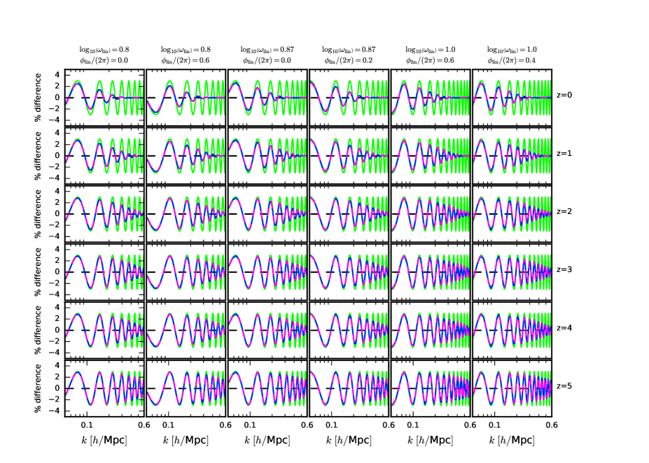
Figure 1: Relative differences with respect to the $\Lambda$CDM matter power spectrum between non-linear matter power spectrum with undamped superimposed oscillation (green), non-linear matter power spectrum obtained from the simulations (blue), and non-linear matter power spectrum reconstructed with our semi-analytical damping (3.2) (dashed magenta) for the template with linear oscillation (2.1) at five different redshift $z=0,1,2,3,4,5$ from the top to the bottom respectively.

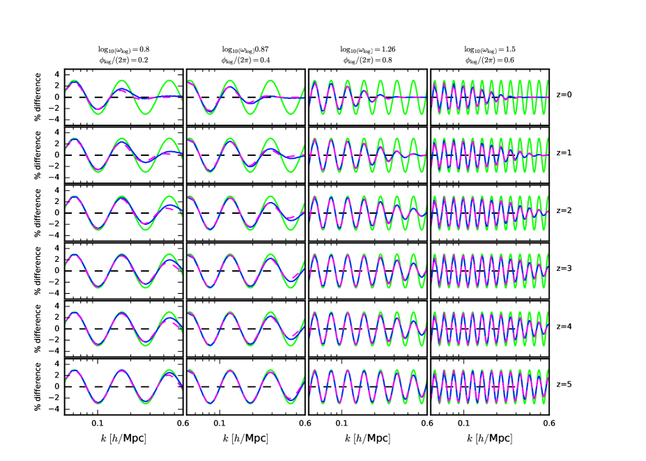
Figure 2: Relative differences with respect to the $\Lambda$CDM matter power spectrum between non-linear matter power spectrum with undamped superimposed oscillation (green), non-linear matter power spectrum obtained from the simulations (blue), and non-linear matter power spectrum reconstructed with our semi-analytical damping (3.2) (dashed magenta) for the template with logarithmic oscillation (2.2) at five different redshift $z=0,1,2,3,4,5$ from the top to the bottom respectively.

All simulations have been run with the N-body code GADGET-3, a modified version of the publicly available numerical code GADGET-2 [47, 48]. The initial conditions have been produced by displacing the DM particles from a cubic Cartesian grid according to second-order Lagrangian Perturbation Theory, with the 2LPTic code [49], at redshift $z=99$. The corresponding input linear matter power spectra were computed with a modified version of the publicly available code CAMB, with the superimposed oscillations given by Eq. (2.1) for the linear cases, and by Eq. (2.2) for logarithmic cases. The values assigned to the amplitude ${\cal A}$, the frequency $\omega$, and the normalized phase $\phi/(2\pi)$, associated with each of the models are reported in Tab. 1. In generating the initial conditions we turned off the Rayleigh sampling as done in Ref. [50], in order to fix the mode amplitude to the expected value of the linear power spectrum. We explicitly check that this aspect does not bias any of our results that are always cast in terms of ratios between the case including primordial oscillations and the corresponding baseline power-law case. For a more comprehensive analysis of Rayleigh sampling and paired fixed field simulation we refer to Ref. [51]. On top of these simulations, we have used a Friends-of-Friends (FoF) algorithm [52] with the standard linking length $b=0.2$, in order to identify particle groups and to extract the statistics of the associated DM halos.

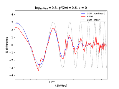
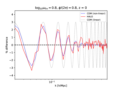
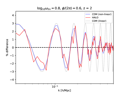
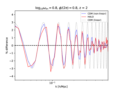
Figure 3: Relative differences with respect to the $\Lambda$CDM case, for the DM halo power spectra computed from N-body simulations (red solid lines), for the template with linear oscillation (2.1) at two different redshift $z=0,2$, from the top to the bottom respectively. We show on the left the results for ${\cal A}_{\rm lin}=0.03$, $\log_{10}\omega_{\rm lin}=0.8$, $\phi/(2\pi)=0.6$ and on the right for ${\cal A}_{\rm lin}=0.03$, $\log_{10}\omega_{\rm lin}=1.0$, $\phi/(2\pi)=0.4$. As a reference, we also plot the corresponding linear (dotted gray lines) and non-linear (blue dashed lines) matter power spectra.

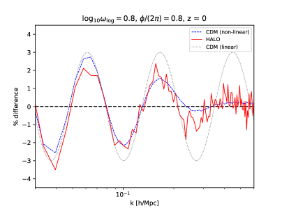
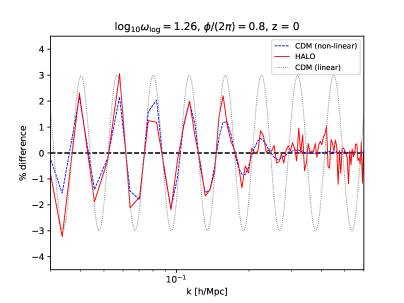
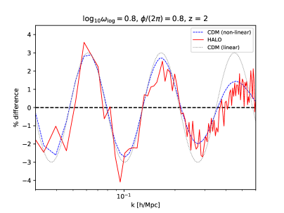
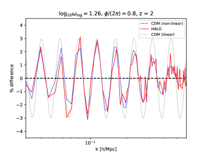
Figure 4: Relative differences with respect to the $\Lambda$CDM case, for the DM halo power spectra computed from N-body simulations (red solid lines), for the template with logarithmic oscillation (2.2) at two different redshift $z=0,2$, from the top to the bottom respectively. We show on the left the results for ${\cal A}_{\rm log}=0.03$, $\log_{10}\omega_{\rm log}=0.8$, $\phi/(2\pi)=0.2$ and on the right for ${\cal A}_{\rm log}=0.03$, $\log_{10}\omega_{\rm log}=1.26$, $\phi/(2\pi)=0.8$. As a reference, we also plot the corresponding linear (dotted gray lines) and non-linear (blue dashed lines) matter power spectra.

For all simulations we have extracted the matter and halo power spectra $P_{m}(k,z)$ and $P_{h}(k,z)$ as a function of the Fourier wavemode $k$ and of the redshift $z$ by assigning the mass of tracer DM particles and individual collapsed halos to a Cartesian grid with $1,024^{3}$ cells through a Cloud-In-Cell mass assignment scheme. The visual inspection of the ratio of each model’s power spectrum to the reference $\Lambda$CDM scenario shows how the primordial pattern of oscillations can still be clearly observed at low redshifts, with a significant damping of the small-scale oscillations which we show between $z=5$ and $z=0$, for both the DM (see Figs. 1 and 2 below) and the halos (see Figs. 3 and 4 below) distributions.

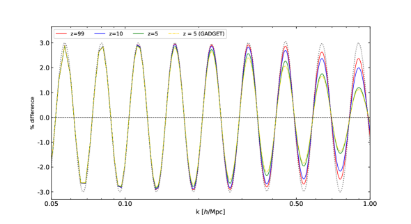
Figure 5: We show the relative differences between the non-linear matter power spectrum of one of the logarithmic models (${\cal A}_{\rm log}=0.03$, $\log_{10}\omega_{\rm log}=0.8$, $\phi_{\rm log}/(2\pi)=0.2$) with respect to the $\Lambda$CDM case, as extracted from initial conditions produced through 2LPTic (solid lines). We also show one power spectrum extracted from the corresponding N-body simulation, at $z=5$ (dot-dashed line). As a reference, we also report the relative difference between the linear matter power spectra (gray dotted line).

In Fig. 5, we show the relative differences between the non-linear matter power spectrum of one of the logarithmic models (${\cal A}_{\rm log}=0.03$, $\log_{10}\omega_{\rm log}=0.8$, $\phi_{\rm log}/(2\pi)=0.2$) with respect to the $\Lambda$CDM case. The solid lines of Fig. 5 refer to spectra extracted from initial conditions produced through 2LPTic, at different redshifts. For comparison, we also show one power spectrum extracted from the corresponding N-body simulation, at $z=5$, which is in very good agreement with the corresponding 2LPTic output (dot-dashed line). The relative difference between the linear matter power spectra is plotted as a gray dotted line.

3.2 Fit model

We use our simulations to calibrate the small-scale damping induced by non-linear dynamics on the oscillatory features superimposed in the matter power spectrum. To do so, we use a least chi-squared method to find the best-fit solution of

$$\chi^{2}\left(\Sigma\right)=\sum_{i}\sum_{z=0}^{5}\sum_{k=k_{\rm min}}^{k_{\rm max}}\left[\frac{P_{i{\rm,fit}}(k,z,\Sigma)-P_{i{\rm,sim}}(k,z)}{\sigma_{i}(k,z)}\right]^{2}$$ (3.1)

with linear loss function, where $i$ runs over the different best-fit for the features parameters listed in Tab. 1, $P_{i{\rm,fit}}(k,z)$ is our semi-analytic template to model non-linear effects for the superimposed oscillations, and $P_{i{\rm,sim}}(k,z)$ is the non-linear matter spectrum from the simulations. We set the variance $\sigma_{i}(k,z)=P_{\rm sim}(k,z)$, where $P_{\rm sim}(k,z)$ is the non-linear matter power spectrum for a $\Lambda$CDM cosmology from the simulations. We consider wavenumbers between $k_{\rm min}=0.05\ h/$Mpc and $k_{\rm max}=0.6\ h/$Mpc.

We write the semi-analytic template to model non-linear effects as:

$$P_{\rm i,fit}(k,z,\Sigma)=P(k,z)\left[1+{\cal A}_{i}\cos\left(\omega_{i}\kappa_{X}+\phi_{i}\right){\cal D}(k,z,\Sigma)\right]\,,$$ (3.2)

where $P(k,z)$ is the non-linear matter power spectrum for a $\Lambda$CDM cosmology from the simulations assuming that the small-scales enhancement of the matter power spectrum and the BAO feature smoothing due to non-linear effects is the same as in $\Lambda$CDM cosmology for this class of models. $\kappa_{\rm lin}\equiv k/k_{*}$ for linear oscillations (2.1) and $\kappa_{\rm log}\equiv\log\left(k/k_{*}\right)$ for logarithmic oscillations (2.2). ${\cal D}(k,z,\Sigma)$ is the damping function to model the damping of superimposed oscillations on the matter power spectrum due to non-linear effects. Analogously to the damping used for BAO [53], we parameterize the damping function with a Gaussian damping as:

$${\cal D}(k,z,\Sigma)=e^{-k^{2}\Sigma^{2}(z)/2}\,,$$ (3.3)

where $\Sigma$ is the redshift-dependent parameter that we fit with our simulations.

The 6 best fitting parameters for the linear feature models given in Tab. 1 are:

$$\Sigma_{\rm lin}(z)=\left[12.23,8.00,5.70,4.40,3.59,3.05\right]\ \text{Mpc}\,,$$

$$\Sigma_{\rm lin}(z)=\left[12.26,8.02,5.73,4.42,3.61,3.06\right]\ \text{Mpc}\,,$$

$$\Sigma_{\rm lin}(z)=\left[12.20,7.96,5.66,4.36,3.55,3.01\right]\ \text{Mpc}\,,$$

$$\Sigma_{\rm lin}(z)=\left[12.26,7.99,5.68,4.38,3.57,3.02\right]\ \text{Mpc}\,,$$

$$\Sigma_{\rm lin}(z)=\left[12.55,8.23,5.88,4.54,3.72,3.17\right]\ \text{Mpc}\,,$$

$$\Sigma_{\rm lin}(z)=\left[12.54,8.21,5.85,4.53,3.71,3.16\right]\ \text{Mpc}\,,$$

where different values inside the square brackets refer to different redshift, i.e. $z=0,1,2,3,4,5$. Fitting simultaneously the 6 best-fit, we find:

$$\Sigma_{\rm lin}(z)=\left[12.34,8.07,5.75,4.44,3.62,3.08\right]\ \text{Mpc}\,.$$ (3.4)

For the 4 best-fit of the logarithmic model (2.2) we obtain:

$$\Sigma_{\rm log}(z)=\left[11.30,6.68,4.47,3.37,2.71,2.27\right]\ \text{Mpc}\,,$$

$$\Sigma_{\rm log}(z)=\left[11.23,6.35,4.09,2.99,2.34,1.91\right]\ \text{Mpc}\,,$$

$$\Sigma_{\rm log}(z)=\left[12.40,7.78,5.35,4.06,3.29,2.77\right]\ \text{Mpc}\,,$$

$$\Sigma_{\rm log}(z)=\left[13.20,8.32,5.74,4.36,3.53,2.98\right]\ \text{Mpc}\,,$$

and fitting simultaneously the 4 best-fit, we find

$$\Sigma_{\rm log}(z)=\left[11.96,7.26,4.90,3.72,3.02,2.55\right]\ \text{Mpc}\,.$$ (3.5)

In Figs. 1-2, we show the comparison between the non-linear matter power spectrum for $\Lambda$CDM obtained from CAMB with undamped superimposed oscillations in green, the non-linear matter power spectrum obtained from the simulations in blue, and the non-linear matter power spectrum for $\Lambda$CDM obtained from CAMB with superimposed oscillations obtained with our fit in dashed magenta for the linear and logarithmic models, respectively with the best-fit (3.4) and (3.5). The fit with the Gaussian envelope in Eq. (3.3) provides an excellent fit to the simulations with relative differences lower than $0.2\%$ for the linear model and $0.6\%$ for the logarithmic one, up to $k\leq 0.6\ h$/Mpc, see left panels on Fig. 6. Note that the absolute variance on the best-fit estimated for $\Sigma_{\rm lin}$ and $\Sigma_{\rm log}$ is smaller then 0.02.

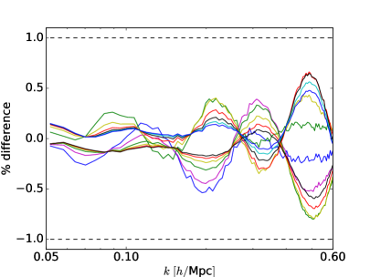
Figure 6: Percentage differences between non-linear matter power spectrum reconstructed with our semi-analytical template (3.2) and the non-linear matter power spectrum obtained from the simulations. We show the results from the Gaussian damping function (3.3) on the left panel for the linear model and on the right panel for the logarithmic model. The semi-analytical non-linear matter power spectra have been calculated using the simultaneous best-fit of the damping parameter $\Sigma$ (3.4)-(3.5).

We then want to compare our findings with the analytic results previously obtained in [25, 26]. The redshift behaviour from our simulations is very well reproduced by the growth factor $G(z)$, i.e. $\Sigma(z)=\Sigma_{\rm nl}G(z)$, as analytically studied in [53, 54]. Based on our Eqs. (3.2)-(3.3), we compare our results for $\Sigma(z)$ with the leading order from perturbation theory [25, 26]:

$$\Sigma_{\rm th}^{2}(k,z)=\frac{1}{3\pi^{2}}\int_{0}^{\Lambda}\mathrm{d}q\left[1-j_{0}(q\omega)+2j_{2}(q\omega)\right]P_{\rm lin}(q,z)\,,$$ (3.6)

where the separation scale $\Lambda$ is suggested to be scale dependent $\Lambda=\epsilon k$ with $\epsilon\in[0.1,0.7]$ [55, 26] and $j_{n}$ are the spherical Bessel function. For the linear template we have $\omega\to\omega_{\rm lin}/(0.05\ \text{Mpc}^{-1})$ and for the logarithmic template $\omega\to\omega_{\rm log}/k$, as derived in [25, 26]. Fig. 7 shows how our estimate for $\Sigma(z)$ is consistent with the analytic estimates to leading order for the linear and logarithmic wiggles according to [25, 26].

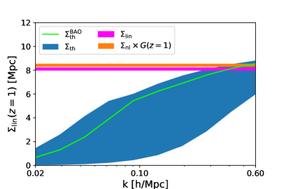
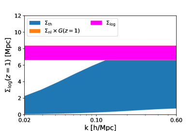
Figure 7: Comparison of our fit for the non-linear damping parameter $\Sigma$ for linear (left panel) and logarithmic (right panel) template of primordial oscillations at redshift $z=1$ with theoretical predictions to leading order [25, 26]. We display $\Sigma(z=1)$ in magenta and $\Sigma_{\rm nl}G(z)$ in orange where $\Sigma(z=1)$ and $\Sigma_{\rm nl}\equiv\Sigma(z=0)$ have been fitted to the N-body simulations. The blue band shows the theoretical prediction to leading order [25, 26] when the separation scale $\Lambda$ varied in the range $(0.1-0.7)\,k$ for the same frequencies of our simulations. We include also the theoretical prediction for the BAO damping with $\omega\sim 110\ \text{Mpc}/h$ (green line) and $\Lambda=0.5\,k$ according to [55].

4 Comparison with the BAO signal

We now want to compare the linear template with the BAO signal. The matter power spectrum can be modeled by a smooth power spectrum without wiggles (nw) plus the BAO spectrum like:

$$P(k,z)\approx P_{\rm nw}(k,z)\left[1+A_{\rm BAO}(k)\sin\left(kr_{s}(z)+\phi\right)\right]\,.$$ (4.1)

The BAO signal in Fourier space looks very similar to the oscillatory pattern induced on the matter power spectrum by the primordial linear oscillations (2.1) with a frequency $\log_{10}\left(\omega_{\rm lin}\right)\sim 0.87$.

As can be seen in Fig. 8, even with a fine tuned frequency, the linear template is different from the BAO signal at early times, i.e. $z=4$: we can see the footprints of the Silk damping on the BAO signal [56], but not on the primordial oscillations.

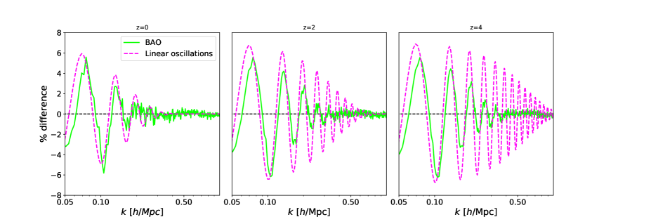
Figure 8: Comparison between the BAO signal at $z=0,\,2,\,4$ (green solid line) extracted from our $\Lambda$CDM simulation and our fit for the linear template with ${\cal A}_{\rm lin}=0.07$, $\log_{10}\left(\omega_{\rm lin}\right)=0.87$, $\phi/(2\pi)=0.4$ (magenta dashed line). The green curve shows the relative differences between the non-linear matter power spectrum with and without BAO wiggles for $\Lambda$CDM (both without superimposed oscillations). The dashed magenta curve shows the relative differences between the non-linear matter power spectrum with and without superimposed linear oscillations (2.1) (both with BAO). We perform the BAO signal subtraction with a polynomial method following Ref. [57]. We tune it in order to have a good BAO signal subtraction and non-distortion of the broadband power spectrum.

As consistency check, we extract the damping of the BAO from our $\Lambda$CDM N-body simulations. We fit BAO non-linear damping by using the Gaussian envelope (3.3):

$$\Sigma_{\rm BAO}(z)=\left[13.90,9.15,6.82,5.66,5.01,4.62\right]\ \text{Mpc}\,.$$ (4.2)

with an absolute variance on the $\Sigma_{\rm BAO}$ estimated smaller than 0.7, which is consistent with results in literature (see for instance Ref. [58]). See Fig. 9 for a comparison of the linear and non-linear BAO signal.

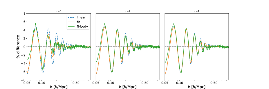
Figure 9: Relative differences between the non-linear matter power spectrum for $\Lambda$CDM with the smooth power spectrum without BAO. The blue dashed curve shows the relative differences for the linear matter power spectrum, the orange curve shows the relative differences for the non-linear matter power spectrum obtained with the Gaussian damping (3.3) with the damping parameter $\Sigma_{\rm BAO}$ (4.2) fitted to the N-body simulations, and the green curve shows the relative differences for the non-linear matter power spectrum extracted from the N-body simulations.

5 Forecast for future galaxy surveys

We describe in this section the Fisher matrix methodology for the galaxy clustering (GC) and the CMB used for our forecasts. We also describe the specifications for the different experiments considered: Euclid-like, Subaru Prime Focus Spectrograph (PFS), Planck-like, and a CMB cosmic-variance (CV) experiment.

5.1 Galaxy power spectrum

We measure galaxy positions in angular and redshift coordinates and not the position in comoving coordinates, i.e. the true galaxy power spectrum is not a direct observable. We use a model for the observed galaxy power spectrum based on [59, 60, 61]:

$$P_{\rm obs}(k^{\rm ref}_{\perp},k^{\rm ref}_{\parallel},z)=\left[\frac{D^{\rm ref}_{\rm A}(z)}{D_{\rm A}(z)}\right]^{2}\frac{H(z)}{H^{\rm ref}(z)}F_{\rm FoG}(k,z)\frac{P_{\rm fit}(k,z)}{\sigma_{8}^{2}(z)}+P_{\rm shot}(z)\,,$$ (5.1)

where $D_{\mathrm{A}}=r(z)/(1+z)$ is the angular diameter distance, $r(z)$ is the comoving distance, $H(z)=\dot{a}/a$ is the Hubble parameter, $k^{2}=k_{\perp}^{2}+k_{\parallel}^{2}$, and $\mu=k_{\parallel}/k=\hat{\bf r}\cdot\hat{\bf k}$. This is connected to the true galaxy power spectrum via a coordinate transformation [62]:

$$k^{\rm ref}_{\perp}=\frac{D_{\rm A}(z)}{D^{\rm ref}_{\rm A}(z)}\,k_{\perp}\,,\qquad k^{\rm ref}_{\parallel}=\frac{H^{\rm ref}(z)}{H(z)}\,k_{\parallel}\,.$$ (5.2)

In Eq. (5.1), $P_{\rm shot}$ is the shot noise and we model the redshift-space distortions (RSD) as:

$$F_{\rm FoG}(k,z)=\frac{\left[b(z)\sigma_{8}(z)+f(z)\sigma_{8}(z)\mu^{2}\right]^{2}}{1+k^{2}\mu^{2}\sigma^{2}_{r,p}/2}e^{-k^{2}\mu^{2}\sigma_{r,z}^{2}}\,,$$ (5.3)

where $b(z)$ is the linear clustering bias, $f(k,z)=\mathrm{d}\ln{G}(k,z)/\mathrm{d}\ln a$ is the growth rate, and $G(k,z)$ is the growth factor. Here the numerator is the linear RSD [63, 64], which takes into account the enhancement due to large-scale peculiar velocities. The Lorentzian denominator models the non-linear damping due to small-scale peculiar velocities, where $\sigma_{r,p}$ is the distance dispersion:

$${\sigma_{r,p}(z)}=\frac{\sigma_{p}(z)}{H(z)a(z)}\,,$$ (5.4)

corresponding to the physical velocity dispersion $\sigma_{p}$. We choose a value of $\sigma_{p}=290$ km/s as our fiducial [61]. An additional exponential damping factor is added to account for the error $\sigma_{z}$ in the determination of the redshift of sources, where:

$$\sigma_{r,z}(z)=\frac{\partial r}{\partial z}\sigma_{z}=\frac{c}{H(z)}\sigma_{z}\,.$$ (5.5)

We model the smearing of the BAO feature according to [53, 61]:

$$P_{\mathrm{dw}}(k,\mu,z)= P_{\mathrm{m}}(k,\mu,z)e^{-\Sigma_{\rm BAO}^{2}(z)k^{2}/2}$$

$$+P_{\mathrm{nw}}(k,\mu,z)\left(1-e^{-\Sigma_{\rm BAO}^{2}(z)k^{2}/2}\right),$$ (5.6)

where $\Sigma_{\rm BAO}(z)\equiv\Sigma_{\rm BAO}G(z)$ with $\Sigma_{\rm BAO}(z=0)=9.3\text{ Mpc}/h$. Here $P_{\mathrm{dw}}$ is dressed with the damped primordial oscillation fitted to the N-body simulations according to Eq. (3.2).

Finally, the finite size of a galaxy survey and the survey window function introduce couplings between different modes $k$ and, as a consequence, discrete bandpowers should be considered in the analysis in order to avoid these correlations. We model the observed matter power spectrum (5.1) in bandpowers averaged over a bandwidth $\Delta k$ with a top-hat window function as in Refs. [12, 25]:

$$\hat{P}_{\rm obs}(k_{i},z)=\frac{1}{\Delta k}\int_{k_{i}-\Delta k/2}^{k_{i}+\Delta k/2}\mathrm{d}k^{\prime}P_{\rm obs}(k^{\prime},z)\,.$$ (5.7)

5.2 Fisher analysis

We follow the same approach as in Ref. [21] (see also Refs. [65, 59]). The Fisher matrix for the observed matter power spectrum (5.1), for a $i$-th redshift bin, is given by:

$$F_{\alpha\beta}^{\rm GC}(z_{i})=\int_{-1}^{1}\mathrm{d}\mu\int_{k_{\rm min}}^{k_{\rm max}}\frac{k^{2}\ \mathrm{d}k}{8\pi^{2}}\frac{\partial\ln P_{\rm obs}(k,\mu,z_{i})}{\partial\alpha}\frac{\partial\ln P_{\rm obs}(k,\mu,z_{i})}{\partial\beta}V_{\rm eff}(z_{i})\,,$$ (5.8)

where $k$ and $\mu$ are the ones related to the reference cosmology, $\partial P_{\rm obs}/\partial\alpha$ is the derivative with respect to the $\alpha$ element in the cosmological parameter vector $\theta$. The effective volume in the $i$-th redshift bin, is given by [66]:

$$V_{\rm eff}(k,\mu,z_{i})\simeq V_{\rm surv}(z_{i})\left[\frac{n(z_{i})P_{\rm obs}(k,\mu;z_{i})}{n(z_{i})P_{\rm obs}(k,\mu,z_{i})+1}\right]^{2}\,,$$ (5.9)

where $V_{\rm surv}(z_{i})$ is the comoving volume in the $i$-th redshift bin.

The full set of parameters $\theta$ includes the standard shape parameters $\big{\{}\omega_{c},\ \omega_{b},\ h,\ n_{s}\big{\}}$, the redshift-depedent parameters $\big{\{}H,D_{\mathrm{A}},\log\left(f\sigma_{8}\right)\big{\}}_{z_{i}}$, the redshift-depedent nuisance parameters $\big{\{}\log\left(b\sigma_{8}\right),\ P_{\rm shot},\ \sigma_{p}\big{\}}_{z_{i}}$ together with the three extra parameters of the primordial oscillatory feature model $\big{\{}{\cal A}_{X},\log_{10}(\omega_{X}),\phi/(2\pi)\big{\}}$ (see Sec. 2). After marginalizing over the nuisance parameters, we project the redshift-dependent parameters on the final set of cosmological parameters

$$\big{\{}\omega_{c},\ \omega_{b},\ h,\ n_{s},\ \ln\left(10^{10}A_{s}\right),{\cal A}_{X},\log_{10}(\omega_{X}),\phi/(2\pi)\big{\}}\,.$$ (5.10)

The Fisher matrix for CMB angular power spectra (temperature and E-mode polarization) is [67, 68, 69, 70, 71]:

$$F_{\alpha\beta}^{\rm CMB}=f_{\rm sky}\sum_{\ell}\frac{2\ell+1}{2}\text{tr}\left[{\bf C}_{\ell,\alpha}{\bf\Sigma}_{\ell}{\bf C}_{\ell,\beta}{\bf\Sigma}_{\ell}\right]\,,$$ (5.11)

where ${\bf C}_{\ell}$ is the covariance matrix, ${\bf C}_{\ell,\alpha}\equiv\partial{\bf C}_{\ell}/\partial\alpha$ is the derivative with respect to the $\alpha$ element in the cosmological parameter vector $\theta$, and ${\bf\Sigma}_{\ell}\equiv\left({\bf C}_{\ell}+{\bf N}_{\ell}\right)^{-1}$ is the inverse of the total noise matrix with ${\bf N}_{\ell}$ the diagonal noise matrix. The effective noise $N^{X}_{\ell}$ is the instrumental noise convolved with the beams of different frequency channels [16]. We adopt the specifications denoted as CMB-1 in [16] for a Planck-like sensitivity, which reproduce uncertainties for standard cosmological parameters similar to those which can be obtained by Planck [72].

We study the predictions for a CV-CMB experiment considering the specifications of $f_{\rm sky}=0.7$, and a multipole range from $\ell_{\rm min}=2$ up to $\ell_{\rm max}=2500$.

The full set of parameters $\theta$ for the CMB includes

$$\big{\{}\omega_{c},\ \omega_{b},\ h,\ n_{s},\ \tau,\ \ln\left(10^{10}A_{s}\right),{\cal A}_{X},\log_{10}(\omega_{X}),\phi_{X}/(2\pi)\big{\}}\,.$$ (5.12)

We marginalize over $\tau$ the Fisher matrix of the CMB before combining it with the one of the GC.

5.3 Galaxy clustering specifications

We focus on two spectroscopic galaxy surveys. First, we consider a Euclid-like spectroscopic survey that will probe $f_{\rm sky}=15,000$ deg² over a redshift range $0.9\leq z\leq 1.8$ divided in 9 tomographic redshift bins equally spaced. We adopt the predicted redshift distribution of the number counts of H$\alpha$-emitting galaxies, dN/dz, per square degree for Euclid-like H$\alpha$-selected survey from Ref. [73] with H$\alpha$ + [NII] blended flux limits of $2\times 10^{-16}$ erg s^-1 cm^-2 and dust method from [74], and the linear clustering bias from Ref. [75]. Secondly, we consider the Subaru Prime Focus Spectrograph (PFS) which will map emission line galaxies spanning a redshift range $0.8<z<2.4$ over 1,464 deg² [76]. In this case, we assume a redshift accuracy of $\sigma_{z}=0.001$ for both the two experiments.

6 Results

We now discuss our results for the two oscillatory models considered (see Sec. 2 for the parameterizations). The marginalized 68% constraints on the amplitude ${\cal A}$ (for different values of $\log_{10}\left(\omega_{X}\right)$ around the best-fit ${\cal A}_{X}=0.03$ and $\phi_{X}/(2\pi)=0.2$) for a Euclid-like experiment are shown in Fig. 10 and can be summarized as follows:

• using the linear matter power spectrum in (5.1), we recover uncertainties on the amplitude consistent with the ones obtained in Ref. [15] for the linear model (2.1) and in Refs. [15, 16] for the logarithmic model (2.2) for $k_{\rm max}=0.1\ h$/Mpc. We find similar uncertainties using the non-linear matter power spectrum when $k_{\rm max}=0.1\ h$/Mpc. This confirms the validity of using the linear theory when restricting to these scales;

• when $k_{\rm max}=0.6\ h$/Mpc, we find that Euclid-like can decrease the uncertainties $\sigma\left({\cal A}\right)$ by a factor 2 when $\log_{10}\left(\omega_{X}\right)>1.0$ thanks to our modelling of non-linear effects. Note that incorrectly by discarting non-linear effects one would get much tighter constraints. We find that a Euclid-like survey can lead to uncertainties which improve on a CV-CMB for $\log_{10}\left(\omega_{\rm lin}\right)>1.3$ and $\log_{10}\left(\omega_{\rm log}\right)>1.6$;

• another interesting aspect is that the improvement in term of uncertainties saturates at $k_{\rm max}=0.3\ h$/Mpc for the model considered. This trend is due to the non-linear damping which smooths most of the oscillations for $k>0.3\ h$/Mpc for $z<2$;

• finally we see that for the linear model the uncertainties for frequencies around the BAO frequency $\log_{10}\left(\omega_{\rm lin}\right)\simeq 0.87$ are sensitively degraded, as pointed out in Ref. [25].

Our best forecasted constraint from Euclid-like GC in combining with CMB-1 (Planck-like) information for both the two models ($X$ = lin, log) corresponds to $\sigma\left({\cal A}_{X}\right)\simeq 0.0018$ for $\log_{10}\left(\omega_{X}\right)=1.1$ and $\sigma\left({\cal A}_{X}\right)\simeq 0.0026$ for $\log_{10}\left(\omega_{X}\right)=2.1$, respectively.

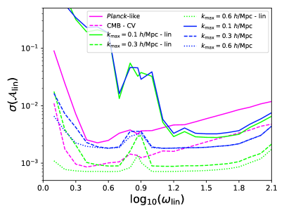
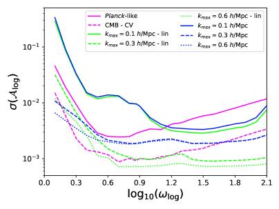
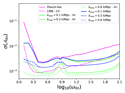
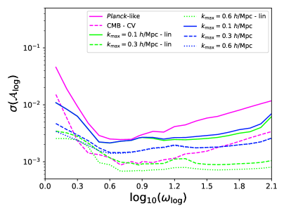
Figure 10: Marginalized uncertainties on ${\cal A}_{X}$ as function of the frequency $\omega_{X}$ for the linear model (left panel) and the logarithmic model (right model). We show uncertainties for CMB-1 (magenta) and for Euclid-like (combined with Planck-like information) in the top (bottom) panels for different maximum wavenumber considered $k_{\rm max}=0.1,0.3,0.6\ h$/Mpc (solid, dashed, dotted). Green lines refer to the linear matter power spectrum in (5.1) and the blue lines to the non-linear matter power spectrum. CMB CV uncertainties are in dashed-magenta.

We then consider PFS. We find also in this case that the improvement in terms of uncertainties saturates around $k_{\rm max}=0.3\ h$/Mpc, even if PFS covers redshifts larger than $z=2$. Despite the smaller sky coverage compared to Euclid (by $\sim 10\%$), we find similar uncertainties for PFS when combined with CMB information, 2 times larger than the uncertainties obtained for the same frequencies for the Euclid-like specifications.

Finally, we combine the two GC clustering experiments with a future full-sky CV-CMB experiment inspired by proposed CMB satellites [77, 78, 79]. Despite the large improvement by a factor of 3 in terms of uncertainties when we consider CMB alone (see Fig. 10), once we combine CMB with GC information the improvement from Planck-like to CV is minor and $\lesssim 10\%$ for $\log_{10}\left(\omega_{X}\right)>1$.

In Fig. 10, we can see that the uncertainties for high frequencies become large. This is due to the window function (5.7) which progressively damp frequencies $\omega_{\rm lin}\gtrsim 0.05/\Delta k$. For $\Delta k\simeq 0.005\,h$/Mpc, close to the fundamental mode of BOSS and PFS, frequencies higher than $\omega_{\rm lin}\sim 10$ start to be damped. For the spectroscopic survey expected for Euclid a smaller bandwidth of $\Delta k\simeq 0.0025$ should guarantee optimal constraints up to $\omega_{\rm lin}\sim 20$. For the logarithmic model the oscillations persist on small scales up to higher frequencies. The addition of the density field reconstruction to the analysis as done in Ref. [25] can further improve the constraints.

7 Conclusions

Global features in the primordial power spectrum provide a variety of information on the physics of the early Universe ranging from the detection of new heaviest particles, of the presence of a fast-roll stage, to fine details in the inflationary dynamics. They can also be used to discriminate between inflation and alternative scenarios in presence of signals which are oscillatory in time.

LSS experiments (also in the perspective of the next coming surveys) give the opportunity to further investigate the presence of any salient features in the matter power spectrum, complementing the constraints based on CMB anisotropy measurements to smaller scales. In Refs. [15, 16, 14, 17, 18, 19, 25], it has been already pointed out the complementarity between the matter power spectrum from future galaxy surveys and the angular power spectrum from the measurements of CMB anisotropies in temperature and polarization to help in characterizing primordial features in the primordial power spectrum. In particular, in Refs. [15, 16] it has been shown how future LSS surveys will be able to improve current constraints on these oscillatory-features models just by using linear scales, i.e. $k\lesssim 0.1\ h$ Mpc^-1.

In order to study the imprints of primordial features on all scales probed by galaxy surveys, we have run a set of high-resolution DM-only cosmological simulations corresponding to different models with linear and logarithmic superimposed oscillations with 1,024³ DM particles in a comoving box with side length of 1,024 Mpc$/h$ and 2,048 Mpc$/h$ (see [24, 20] for previous applications of N-body simulations to different models of primordial features). Our study is important to understand the fully non-linear regime for the clustering in models with primordial features. Our results complement analytic approximations based on a perturbative treatment, see Refs. [24, 25, 26], and show a compatible non-linear damping with respect to analytic results to leading order. We stress that these effects are relevant for current galaxy surveys like BOSS and eBOSS [80], DESI [81], DES [82], as well as for future experiments such as Euclid and PSF-Subaru.

After calibrating the damping of the primordial oscillations with a semi-analytical template (3.3) against the matter power spectrum extracted from the N-body simulations at different redshifts, we have studied the forecasted uncertainties extending our previous analysis [16] on the capability of GC up to quasi-linear scales $k\lesssim 0.1\ h/$Mpc to improve the uncertainties for such class of primordial models. The uncertainties on the amplitude of the linear (logarithmic) primordial oscillations for a wide Euclid-like experiment covering the redshift range $0.9\leq z\leq 1.8$ over a sky patch of 15,000 deg² around a fiducial value ${\cal A}_{\rm lin}=0.03$ $\left({\cal A}_{\rm log}=0.03\right)$ are $\sigma\left({\cal A}_{X}\right)\simeq 0.0025\ (0.0034)$ for $\log_{10}\left(\omega_{X}\right)=0.1$, $\sigma\left({\cal A}_{X}\right)\simeq 0.0017\ (0.0018)$ for $\log_{10}\left(\omega_{X}\right)=1.1$, $\sigma\left({\cal A}_{X}\right)\simeq 0.0041\ (0.0026)$ for $\log_{10}\left(\omega_{X}\right)=2.1$ and for a deeper experiment as PFS covering the redshift range $0.8\leq z\leq 2.4$ over a sky patch of 1,464 deg² are $\sigma\left({\cal A}_{X}\right)\simeq 0.0044\ (0.0032)$ for $\log_{10}\left(\omega_{X}\right)=0.1$, $\sigma\left({\cal A}_{X}\right)\simeq 0.0026\ (0.0029)$ for $\log_{10}\left(\omega_{X}\right)=1.1$, $\sigma\left({\cal A}_{X}\right)\simeq 0.0096\ (0.0064)$ for $\log_{10}\left(\omega_{X}\right)=2.1$, in combination with Planck-like CMB temperature and polarization anisotropies and assuming $k_{\rm max}=0.6\ h/$Mpc. We find an improvement by a factor 2 including non-linear scales from $k_{\rm max}=0.1\ h/$Mpc to $k_{\rm max}=0.6\ h/$Mpc.

Oscillatory features in the PPS also generate highly correlated signals in terms of non-Gaussianities [83, 27, 84, 85] and specific features appear also in the bispectrum (see Ref. [86] for a review), so that primordial features can also be searched for in the bispectrum [87], or jointly in the power spectrum and bispectrum [88, 89, 90]. In addition, a scale-dependent contribution to the clustering bias is expected in the presence of primordial non-Gaussianity [91, 92, 93, 94]. This last effect has been studied in Ref. [21] for large-scale features and in Ref. [95] for oscillatory features resulting in a very small effect that upcoming surveys will be unable to detect. Direct studies of the imprint from these oscillatory features on the matter bispectrum are still promising in order to have a tighter and more robust detection of this features. A first investigation of the matter bispectrum in these models has been presented in Ref. [26] using perturbation theory, and it will be important to further extend this framework in order to see how non-linearities affect higher-order statistics.

References

- [1] J. Chluba, J. Hamann and S. P. Patil, Int. J. Mod. Phys. D 24 (2015) no.10, 1530023 doi:10.1142/S0218271815300232 [arXiv:1505.01834 [astro-ph.CO]].
- [2] A. A. Starobinsky, Phys. Lett. 91B (1980) 99 [Adv. Ser. Astrophys. Cosmol. 3 (1987) 130]. doi:10.1016/0370-2693(80)90670-X
- [3] A. H. Guth, Phys. Rev. D 23 (1981) 347 [Adv. Ser. Astrophys. Cosmol. 3 (1987) 139]. doi:10.1103/PhysRevD.23.347
- [4] A. D. Linde, Phys. Lett. 108B (1982) 389 [Adv. Ser. Astrophys. Cosmol. 3 (1987) 149]. doi:10.1016/0370-2693(82)91219-9
- [5] A. D. Linde, Phys. Lett. 129B (1983) 177. doi:10.1016/0370-2693(83)90837-7
- [6] A. Albrecht and P. J. Steinhardt, Phys. Rev. Lett. 48 (1982) 1220 [Adv. Ser. Astrophys. Cosmol. 3 (1987) 158]. doi:10.1103/PhysRevLett.48.1220
- [7] X. Chen and Y. Wang, JCAP 1004, 027 (2010) doi:10.1088/1475-7516/2010/04/027 [arXiv:0911.3380 [hep-th]].
- [8] N. Arkani-Hamed and J. Maldacena, arXiv:1503.08043 [hep-th].
- [9] H. V. Peiris et al. [WMAP Collaboration], Astrophys. J. Suppl. 148 (2003) 213 doi:10.1086/377228 [astro-ph/0302225].
- [10] Y. Akrami et al. [Planck Collaboration], arXiv:1807.06211 [astro-ph.CO].
- [11] H. Zhan, L. Knox, A. Tyson and V. Margoniner, Astrophys. J. 640 (2006) 8 doi:10.1086/500077 [astro-ph/0508119].
- [12] Z. Huang, L. Verde and F. Vernizzi, JCAP 1204 (2012) 005 doi:10.1088/1475-7516/2012/04/005 [arXiv:1201.5955 [astro-ph.CO]].
- [13] B. Hu and J. Torrado, Phys. Rev. D 91 (2015) no.6, 064039 doi:10.1103/PhysRevD.91.064039 [arXiv:1410.4804 [astro-ph.CO]].
- [14] X. Chen, P. D. Meerburg and M. Münchmeyer, JCAP 1609 (2016) no.09, 023 doi:10.1088/1475-7516/2016/09/023 [arXiv:1605.09364 [astro-ph.CO]].
- [15] X. Chen, C. Dvorkin, Z. Huang, M. H. Namjoo and L. Verde, JCAP 1611 (2016) no.11, 014 doi:10.1088/1475-7516/2016/11/014 [arXiv:1605.09365 [astro-ph.CO]].
- [16] M. Ballardini, F. Finelli, C. Fedeli and L. Moscardini, JCAP 1610 (2016) 041 Erratum: [JCAP 1804 (2018) no.04, E01] doi:10.1088/1475-7516/2018/04/E01, 10.1088/1475-7516/2016/10/041 [arXiv:1606.03747 [astro-ph.CO]].
- [17] Y. Xu, J. Hamann and X. Chen, Phys. Rev. D 94 (2016) no.12, 123518 doi:10.1103/PhysRevD.94.123518 [arXiv:1607.00817 [astro-ph.CO]].
- [18] M. A. Fard and S. Baghram, JCAP 1801 (2018) no.01, 051 doi:10.1088/1475-7516/2018/01/051 [arXiv:1709.05323 [astro-ph.CO]].
- [19] G. A. Palma, D. Sapone and S. Sypsas, JCAP 1806 (2018) no.06, 004 doi:10.1088/1475-7516/2018/06/004 [arXiv:1710.02570 [astro-ph.CO]].
- [20] B. L’Huillier, A. Shafieloo, D. K. Hazra, G. F. Smoot and A. A. Starobinsky, Mon. Not. Roy. Astron. Soc. 477 (2018) no.2, 2503 doi:10.1093/mnras/sty745 [arXiv:1710.10987 [astro-ph.CO]].
- [21] M. Ballardini, F. Finelli, R. Maartens and L. Moscardini, JCAP 1804 (2018) no.04, 044 doi:10.1088/1475-7516/2018/04/044 [arXiv:1712.07425 [astro-ph.CO]].
- [22] M. Ballardini, Phys. Dark Univ. 23 (2019) 100245 doi:10.1016/j.dark.2018.11.006 [arXiv:1807.05521 [astro-ph.CO]].
- [23] C. Zeng, E. D. Kovetz, X. Chen, Y. Gong, J. B. Muñoz and M. Kamionkowski, Phys. Rev. D 99 (2019) no.4, 043517 doi:10.1103/PhysRevD.99.043517 [arXiv:1812.05105 [astro-ph.CO]].
- [24] Z. Vlah, U. Seljak, M. Y. Chu and Y. Feng, JCAP 1603 (2016) no.03, 057 doi:10.1088/1475-7516/2016/03/057 [arXiv:1509.02120 [astro-ph.CO]].
- [25] F. Beutler, M. Biagetti, D. Green, A. Slosar and B. Wallisch, arXiv:1906.08758 [astro-ph.CO].
- [26] A. Vasudevan, M. M. Ivanov, S. Sibiryakov and J. Lesgourgues, JCAP 1909 (2019) no.09, 037 doi:10.1088/1475-7516/2019/09/037 [arXiv:1906.08697 [astro-ph.CO]].
- [27] X. Chen, R. Easther and E. A. Lim, JCAP 0804 (2008) 010 doi:10.1088/1475-7516/2008/04/010 [arXiv:0801.3295 [astro-ph]].
- [28] X. Wang, B. Feng, M. Li, X. L. Chen and X. Zhang, Int. J. Mod. Phys. D 14 (2005) 1347 doi:10.1142/S0218271805006985 [astro-ph/0209242].
- [29] R. Bean, X. Chen, G. Hailu, S.-H. H. Tye and J. Xu, JCAP 0803 (2008) 026 doi:10.1088/1475-7516/2008/03/026 [arXiv:0802.0491 [hep-th]].
- [30] R. Flauger, L. McAllister, E. Pajer, A. Westphal and G. Xu, JCAP 1006 (2010) 009 doi:10.1088/1475-7516/2010/06/009 [arXiv:0907.2916 [hep-th]].
- [31] X. Chen, Phys. Lett. B 706 (2011) 111 doi:10.1016/j.physletb.2011.11.009 [arXiv:1106.1635 [astro-ph.CO]].
- [32] X. Chen, JCAP 1201 (2012) 038 doi:10.1088/1475-7516/2012/01/038 [arXiv:1104.1323 [hep-th]].
- [33] U. H. Danielsson, Phys. Rev. D 66 (2002) 023511 doi:10.1103/PhysRevD.66.023511 [hep-th/0203198].
- [34] R. Easther, B. R. Greene, W. H. Kinney and G. Shiu, Phys. Rev. D 66 (2002) 023518 doi:10.1103/PhysRevD.66.023518 [hep-th/0204129].
- [35] J. Martin and R. Brandenberger, Phys. Rev. D 68 (2003) 063513 doi:10.1103/PhysRevD.68.063513 [hep-th/0305161].
- [36] R. E. Smith et al. [VIRGO Consortium], Mon. Not. Roy. Astron. Soc. 341 (2003) 1311 doi:10.1046/j.1365-8711.2003.06503.x [astro-ph/0207664].
- [37] R. Takahashi, M. Sato, T. Nishimichi, A. Taruya and M. Oguri, Astrophys. J. 761 (2012) 152 doi:10.1088/0004-637X/761/2/152 [arXiv:1208.2701 [astro-ph.CO]].
- [38] A. Mead, J. Peacock, C. Heymans, S. Joudaki and A. Heavens, Mon. Not. Roy. Astron. Soc. 454 (2015) no.2, 1958 doi:10.1093/mnras/stv2036 [arXiv:1505.07833 [astro-ph.CO]].
- [39] A. Mead, C. Heymans, L. Lombriser, J. Peacock, O. Steele and H. Winther, Mon. Not. Roy. Astron. Soc. 459 (2016) no.2, 1468 doi:10.1093/mnras/stw681 [arXiv:1602.02154 [astro-ph.CO]].
- [40] A. A. Starobinsky, JETP Lett. 55, 489 (1992) [Pisma Zh. Eksp. Teor. Fiz. 55, 477 (1992)].
- [41] J. A. Adams, B. Cresswell and R. Easther, Phys. Rev. D 64, 123514 (2001) doi:10.1103/PhysRevD.64.123514 [astro-ph/0102236].
- [42] A. Lewis, A. Challinor and A. Lasenby, Astrophys. J. 538 (2000) 473 doi:10.1086/309179 [astro-ph/9911177].
- [43] C. Howlett, A. Lewis, A. Hall and A. Challinor, JCAP 1204 (2012) 027 doi:10.1088/1475-7516/2012/04/027 [arXiv:1201.3654 [astro-ph.CO]].
- [44] J. Lesgourgues, arXiv:1104.2932 [astro-ph.IM].
- [45] D. Blas, J. Lesgourgues and T. Tram, JCAP 1107 (2011) 034 doi:10.1088/1475-7516/2011/07/034 [arXiv:1104.2933 [astro-ph.CO]].
- [46] S. Bird, M. Viel and M. G. Haehnelt, Mon. Not. Roy. Astron. Soc. 420 (2012) 2551 doi:10.1111/j.1365-2966.2011.20222.x [arXiv:1109.4416 [astro-ph.CO]].
- [47] V. Springel, S. D. M. White, G. Tormen and G. Kauffmann, Mon. Not. Roy. Astron. Soc. 328 (2001) 726 doi:10.1046/j.1365-8711.2001.04912.x [astro-ph/0012055].
- [48] V. Springel, Mon. Not. Roy. Astron. Soc. 364 (2005) 1105 doi:10.1111/j.1365-2966.2005.09655.x [astro-ph/0505010].
- [49] M. Crocce, S. Pueblas and R. Scoccimarro, Mon. Not. Roy. Astron. Soc. 373 (2006) 369 doi:10.1111/j.1365-2966.2006.11040.x [astro-ph/0606505].
- [50] M. Viel, M. G. Haehnelt and V. Springel, JCAP 1006 (2010) 015 doi:10.1088/1475-7516/2010/06/015 [arXiv:1003.2422 [astro-ph.CO]].
- [51] F. Villaescusa-Navarro et al., Astrophys. J. 867 (2018) no.2, 137 doi:10.3847/1538-4357/aae52b [arXiv:1806.01871 [astro-ph.CO]].
- [52] M. Davis, G. Efstathiou, C. S. Frenk and S. D. M. White, Astrophys. J. 292 (1985) 371. doi:10.1086/163168
- [53] H. J. Seo and D. J. Eisenstein, Astrophys. J. 665 (2007) 14 doi:10.1086/519549 [astro-ph/0701079].
- [54] D. Blas, M. Garny, M. M. Ivanov and S. Sibiryakov, JCAP 1607 (2016) 028 doi:10.1088/1475-7516/2016/07/028 [arXiv:1605.02149 [astro-ph.CO]].
- [55] T. Baldauf, M. Mirbabayi, M. Simonović and M. Zaldarriaga, Phys. Rev. D 92 (2015) no.4, 043514 doi:10.1103/PhysRevD.92.043514 [arXiv:1504.04366 [astro-ph.CO]].
- [56] J. Silk, Astrophys. J. 151 (1968) 459. doi:10.1086/149449
- [57] S. R. Hinton et al., Mon. Not. Roy. Astron. Soc. 464 (2017) no.4, 4807 doi:10.1093/mnras/stw2725 [arXiv:1611.08040 [astro-ph.CO]].
- [58] Z. Ding, H. J. Seo, Z. Vlah, Y. Feng, M. Schmittfull and F. Beutler, Mon. Not. Roy. Astron. Soc. 479 (2018) no.1, 1021 doi:10.1093/mnras/sty1413 [arXiv:1708.01297 [astro-ph.CO]].
- [59] H. J. Seo and D. J. Eisenstein, Astrophys. J. 598 (2003) 720 doi:10.1086/379122 [astro-ph/0307460].
- [60] Y. S. Song and W. J. Percival, JCAP 0910 (2009) 004 doi:10.1088/1475-7516/2009/10/004 [arXiv:0807.0810 [astro-ph]].
- [61] Y. Wang, C. H. Chuang and C. M. Hirata, Mon. Not. Roy. Astron. Soc. 430 (2013) 2446 doi:10.1093/mnras/stt068 [arXiv:1211.0532 [astro-ph.CO]].
- [62] C. Alcock and B. Paczynski, Nature 281 (1979) 358. doi:10.1038/281358a0
- [63] N. Kaiser, Mon. Not. Roy. Astron. Soc. 227 (1987) 1.
- [64] A. J. S. Hamilton, doi:10.1007/978-94-011-4960-0_17 astro-ph/9708102.
- [65] M. Tegmark, Phys. Rev. Lett. 79 (1997) 3806 doi:10.1103/PhysRevLett.79.3806 [astro-ph/9706198].
- [66] H. A. Feldman, N. Kaiser and J. A. Peacock, Astrophys. J. 426 (1994) 23 doi:10.1086/174036 [astro-ph/9304022].
- [67] L. Knox, Phys. Rev. D 52 (1995) 4307 doi:10.1103/PhysRevD.52.4307 [astro-ph/9504054].
- [68] G. Jungman, M. Kamionkowski, A. Kosowsky and D. N. Spergel, Phys. Rev. D 54 (1996) 1332 doi:10.1103/PhysRevD.54.1332 [astro-ph/9512139].
- [69] U. Seljak, Astrophys. J. 482 (1997) 6 doi:10.1086/304123 [astro-ph/9608131].
- [70] M. Zaldarriaga and U. Seljak, Phys. Rev. D 55 (1997) 1830 doi:10.1103/PhysRevD.55.1830 [astro-ph/9609170].
- [71] M. Kamionkowski, A. Kosowsky and A. Stebbins, Phys. Rev. D 55 (1997) 7368 doi:10.1103/PhysRevD.55.7368 [astro-ph/9611125].
- [72] Y. Akrami et al. [Planck Collaboration], arXiv:1807.06205 [astro-ph.CO].
- [73] A. Merson, Y. Wang, A. Benson, A. Faisst, D. Masters, A. Kiessling and J. Rhodes, Mon. Not. Roy. Astron. Soc. 474 (2018) no.1, 177 doi:10.1093/mnras/stx2649 [arXiv:1710.00833 [astro-ph.GA]].
- [74] D. Calzetti, L. Armus, R. C. Bohlin, A. L. Kinney, J. Koornneef and T. Storchi-Bergmann, Astrophys. J. 533 (2000) 682 doi:10.1086/308692 [astro-ph/9911459].
- [75] A. Merson, A. Smith, A. Benson, Y. Wang and C. M. Baugh, 2019, Monthly Notices of the Royal Astronomical Society, Volume 486, Issue 4, p.5737-5765 doi:10.1093/mnras/stz1204 [arXiv:1903.02030 [astro-ph.CO]].
- [76] R. Ellis et al. [PFS Team], Publ. Astron. Soc. Jap. 66 (2014) no.1, R1 doi:10.1093/pasj/pst019 [arXiv:1206.0737 [astro-ph.CO]].
- [77] F. Finelli et al. [CORE Collaboration], JCAP 1804 (2018) 016 doi:10.1088/1475-7516/2018/04/016 [arXiv:1612.08270 [astro-ph.CO]].
- [78] S. Hanany et al. [NASA PICO Collaboration], arXiv:1902.10541 [astro-ph.IM].
- [79] J. Delabrouille et al., arXiv:1909.01591 [astro-ph.CO].
- [80] S. Alam et al. [BOSS Collaboration], Mon. Not. Roy. Astron. Soc. 470 (2017) no.3, 2617 doi:10.1093/mnras/stx721 [arXiv:1607.03155 [astro-ph.CO]].
- [81] A. Aghamousa et al. [DESI Collaboration], 2016, arXiv e-prints, arXiv:1611.00036
- [82] J. Elvin-Poole et al. [DES Collaboration], Phys. Rev. D 98 (2018) no.4, 042006 doi:10.1103/PhysRevD.98.042006 [arXiv:1708.01536 [astro-ph.CO]].
- [83] X. Chen, R. Easther and E. A. Lim, JCAP 0706 (2007) 023 doi:10.1088/1475-7516/2007/06/023 [astro-ph/0611645].
- [84] R. Flauger and E. Pajer, JCAP 1101 (2011) 017 doi:10.1088/1475-7516/2011/01/017 [arXiv:1002.0833 [hep-th]].
- [85] X. Chen, JCAP 1012 (2010) 003 doi:10.1088/1475-7516/2010/12/003 [arXiv:1008.2485 [hep-th]].
- [86] X. Chen, Adv. Astron. 2010 (2010) 638979 doi:10.1155/2010/638979 [arXiv:1002.1416 [astro-ph.CO]].
- [87] Y. Akrami et al. [Planck Collaboration], arXiv:1905.05697 [astro-ph.CO].
- [88] J. R. Fergusson, H. F. Gruetjen, E. P. S. Shellard and B. Wallisch, Phys. Rev. D 91 (2015) no.12, 123506 doi:10.1103/PhysRevD.91.123506 [arXiv:1412.6152 [astro-ph.CO]].
- [89] P. D. Meerburg, M. Münchmeyer and B. Wandelt, Phys. Rev. D 93 (2016) no.4, 043536 doi:10.1103/PhysRevD.93.043536 [arXiv:1510.01756 [astro-ph.CO]].
- [90] D. Karagiannis, A. Lazanu, M. Liguori, A. Raccanelli, N. Bartolo and L. Verde, Mon. Not. Roy. Astron. Soc. 478 (2018) no.1, 1341 doi:10.1093/mnras/sty1029 [arXiv:1801.09280 [astro-ph.CO]].
- [91] N. Dalal, O. Dore, D. Huterer and A. Shirokov, Phys. Rev. D 77 (2008) 123514 doi:10.1103/PhysRevD.77.123514 [arXiv:0710.4560 [astro-ph]].
- [92] S. Matarrese and L. Verde, Astrophys. J. 677 (2008) L77 doi:10.1086/587840 [arXiv:0801.4826 [astro-ph]].
- [93] V. Desjacques, U. Seljak and I. Iliev, Mon. Not. Roy. Astron. Soc. 396 (2009) 85 doi:10.1111/j.1365-2966.2009.14721.x [arXiv:0811.2748 [astro-ph]].
- [94] A. Slosar, C. Hirata, U. Seljak, S. Ho and N. Padmanabhan, JCAP 0808 (2008) 031 doi:10.1088/1475-7516/2008/08/031 [arXiv:0805.3580 [astro-ph]].
- [95] G. Cabass, E. Pajer and F. Schmidt, JCAP 1809 (2018) no.09, 003 doi:10.1088/1475-7516/2018/09/003 [arXiv:1804.07295 [astro-ph.CO]].