OPTICAL TRANSMISSION SPECTRA OF HOT-JUPITERS: EFFECTS OF SCATTERING

Abstract

We present new grids of transmission spectra for hot-Jupiters by solving the multiple scattering radiative transfer equations with non-zero scattering albedo instead of using the Beer-Bouguer-Lambert law for the change in the transmitted stellar intensity. The diffused reflection and transmission due to scattering increases the transmitted stellar flux resulting into a decrease in the transmission depth. Thus we demonstrate that scattering plays a double role in determining the optical transmission spectra – increasing the total optical depth of the medium and adding the diffused radiation due to scattering to the transmitted stellar radiation. The resulting effects yield into an increase in the transmitted flux and hence reduction in the transmission depth. For a cloudless planetary atmosphere, Rayleigh scattering albedo alters the transmission depth up to about 0.6 micron but the change in the transmission depth due to forward scattering by cloud or haze is significant throughout the optical and near-infrared regions. However, at wavelength longer than about 1.2 $\mu$m, the scattering albedo becomes negligible and hence the transmission spectra match with that calculated without solving the radiative transfer equations. We compare our model spectra with existing theoretical models and find significant difference at wavelength shorter than one micron. We also compare our models with observational data for a few hot-Jupiters which may help constructing better retrieval models in future.

1 Introduction

While planetary transit photometry provides important physical properties of exoplanets, it cannot explore the planetary atmosphere. As pointed out for the first time by Seager & Sasselov (2000), it is the transmission spectroscopic method that can probe the physical and chemical properties of the atmosphere of exoplanets having near edge-on orientation.

During the transit epoch of an exoplanet across its parent star, a part of the starlight passes through the planetary atmosphere. The interaction of this star-light with the atmospheric material through absorption and scattering is imprinted on top of the stellar spectra. A correct interpretation of this transmission spectra needs a comparison with a consistent theoretical model that incorporates all the physical and chemical processes in the planetary atmosphere.

Theoretical models for transmission spectra of stars with transiting exoplanets having a wide range of equilibrium temperature and surface gravity have already been presented by several groups, e.g. (Brown, 2001; Tinetti, Liang, et al., 2007; Madhusudhan and Seager, 2009; Burrows et al., 2010; Fortney, Shabram, Showman et al., 2010; Griffith, 2014; Waldmann, Tinetti, Rocchetto, et al., 2015; Kempton, Lupu, Owusu-Asare et al., 2017; Barstow, Aigrain, Irwin et al.,, 2017; Heng et al., 2018; Goyal, Mayne, Sing et al., 2018; Goyal, Wakeford, Mayne et al., 2019). Useful review and overview on modeling exoplanetary atmosphere can be found in Fortney (2018); Burrows, (2014); Tinetti, Encrenaz & Coustenis (2013).

The models by Fortney, Shabram, Showman et al. (2010) and Kempton, Lupu, Owusu-Asare et al. (2017) are based on thermo-chemical equilibrium scheme, use elemental abundances from Lodders, K. (2003) and atomic-molecular line-list primarily from HITRAN (Gordon et al., 2017). On the other hand, model by Goyal, Wakeford, Mayne et al. (2019); Goyal, Mayne, Sing et al. (2018) uses elemental abundances from Asplund, Grevesse, Sauval & Scott (2009) and the line-list from Exomol (Tennyson, Yurchenko, Al-Refaie, et al., 2016). Nevertheless all the three models agrees well at low temperature.

In all these three models and the other models mentioned above, only absorption of starlight passing through the planetary atmosphere is incorporated and thus the reduced intensity $I$ due to the interaction of atoms and molecules in the atmosphere is calculated by using the Beer-Bouguer-Lambert law $I=I_{0}e^{-\tau}$ where $I_{0}$ is the incident stellar intensity and $\tau$ is the line-of-sight optical depth of the medium that imprint the signature of the planetary atmosphere. In these models, although opacity due to scattering is added up to the opacity due to true absorption, angular distribution of the transmitting photon due to scattering is not incorporated. Since scattering co-efficient and hence single scattering albedo at longer wavelengths, e.g., in infrared is extremely small or zero, this approximation is valid at wavelengths beyond the optical region. But it overestimates the transmission depth at shorter wavelength and hence does not provide correct results for optical region where scattering albedo is comparable to 1 and the diffused transmission and reflection due to scattering plays important role in determining the radiation field. A correct treatment is thus to solve the multi-scattering radiative transfer equations for the diffused reflection and transmission as demonstrated by de Kok & Stam (2012) who presented three dimensional Monte Carlo simulation for Titan’s atmosphere at wavelengths ranging between 2.0 and 2.8 micron and reported significant underestimation in the calculation of the transmission flux if forward scattering by haze and gas is neglected in the retrieval models.

In this paper we present the transmission depth as the solution of the detail multiple-scattering radiative transfer equations for the atmosphere of exoplanets with a wide range of equilibrium temperature and surface gravity.

Today a few tens of gaseous exoplanet atmospheres have been probed in the optical and near-IR through transit observations with the Wide Field Camera 3 on board Hubble Space Telescope (Tsiaras, Waldmann, et al., 2018). For a sub-sample of those, also optical spectra using the Space Telescope Imaging Spectrograph are available (Sing, Fortney, Nikolov et al., 2016). This survey was complemented by photometric transit observations at two more longer wavelengths 3.6 $\mu m$ and 4.5 $\mu m$ by using the Spitzer Space Telescope Infrared Array Camera. Although one needs to be careful in combining data from multiple instruments (Yip et al., 2019), these observational data provide an excellent opportunity to understand the scope and limitations of various theoretical models.

We compare our model spectra with the existing theoretical models and with the observed HST and Spitzer data. In the next section we provide the formalisms for calculating the transmission depth. In Section 3 we discuss the model absorption and scattering opacity adopted in our present models. Section 4 outlines the numerical method for solving the multiple scattering radiative transfer equations. The non-isothermal temperature-pressure profiles for non-Grey planetary atmosphere used in our models are described in Section 5. In Section 6 we present a simple haze model that is incorporated in order to include additional absorption and scattering opacities. The results are discussed in Section 7 followed by specific conclusion in the last section.

2 The Transmission Depth

The transmission spectra of exoplanets are expressed in term of the wavelength dependent transmission depth which is given by Kempton, Lupu, Owusu-Asare et al. (2017)

$$D_{\lambda}=1-\frac{F_{in}}{F_{out}},$$ (1)

where $F_{out}=F_{\star}$ is the out-of-transit stellar flux. The in-transit stellar flux $F_{in}$ which is the flux of the host star that transmits through the planetary atmosphere is given by

$$F_{in}=\left(1-\frac{R_{PA}^{2}}{R_{\star}^{2}}\right)F_{\star}+F_{P},$$ (2)

where $R_{PA}$ is the combined base radius $R_{P}$ of the planet and its atmosphere, $R_{\star}$ is the radius of the host star and $F_{P}$ is the additional stellar flux that passes through the planetary atmosphere and suffers absorption and scattering. Clearly, the first term in the right hand side of the above expression represents the stellar radiation during the transit of the planet and its atmosphere and the second term represents the additional stellar radiation filtered through the planetary atmosphere. The base radius $R_{P}$ is the planetary radius at which the planet becomes opaque at all wavelength. For a rocky planet, $R_{P}$ is the distance between the center to the planetary surface. But for gaseous planets, $R_{P}$ is the height of the region bellow which no radiation can transmit from.

From the above equations, the transmission depth can be written in a simple form

$$D_{\lambda}=\frac{R_{PA}^{2}}{R_{\star}^{2}}-\frac{F_{P}}{F_{\star}}.$$ (3)

Sometimes the transmission spectra is expressed in terms of the wavelength dependent planet-to-star radius ratio which is the square root of $D_{\lambda}$.

The stellar radiation $F_{P}$ that filters through the planetary atmosphere is calculated from the incident stellar intensity. If the calculations of transmission spectra assumes only absorption of starlight passing through the planetary atmosphere, Beer-Bouguer-Lambert law can be used which is given by

$$I(\lambda)=I_{0}(\lambda)e^{-\tau_{\lambda}/\mu_{0}},$$ (4)

where $I_{0}$ is the intensity of the incident stellar radiation, $I$ is the stellar intensity filtered through the planetary atmosphere, $\tau$ is the optical depth along the ray path and $\mu_{0}$ is the cosine of the angle between the direction of the incident starlight and the normal to the planetary surface. Due to the edge on orientation, $\mu_{0}=1$ is adopted in the present investigation such that the starlight during planetary transit always incident along the normal to the planetary atmosphere.

Although in many previous models, opacity due to scattering $\sigma$ is added to the true absorption $\kappa$, scattering into and out of the ray is not explicitly considered before. This assumption is reasonable for calculating the transmission spectra at longer wavelength, e.g., in the infra-red region where the scattering albedo is negligible. But it grossly overestimate the transmission depth and hence does not provide correct results for optical region where scattering albedo $\omega$ which is the ratio of the scattering co-efficient to the extinction coefficient is non-zero and plays important role in determining the radiation field. It’s worth mentioning that $\omega$ depends on the wavelength as well as the atmospheric depth. A true treatment is thus to solve the multi-scattering radiative transfer equations for diffused reflection and transmission which for a plane-parallel geometry is given by Chandrasekhar (1960)

where $I(\tau,\mu,\lambda)$ is the specific intensity of the diffused radiation field along the direction $\mu=\cos\theta$, $\theta$ being the angle between the axis of symmetry and the ray path, $F$ is the incident stellar flux in the direction $-\mu_{0}$, $\omega$ is the albedo for single scattering, $p(\mu,\mu^{\prime})$ is the scattering phase function that describes the angular distribution of the photon before and after scattering and $\tau$ is the optical depth along the line of sight given by Tinetti, Encrenaz & Coustenis (2013)

$$\tau(\lambda,z)=2\int_{0}^{l(z)}{\chi(\lambda,z)\rho(z)\text{d}l}.$$ (6)

In the above equation $\chi$ is the extinction co-efficient which is the sum of the absorption coefficient $\kappa$ and scattering co-efficient $\sigma$, $\rho(z)$ is the atmospheric density, $z$ is the atmospheric height along the axis of symmetry of the planet and $l$ is the path traveled by the stellar photon and can be written as (Tinetti, Encrenaz & Coustenis, 2013)

$$l(z)=\int{\text{d}l}=\sqrt{(R_{P}+z_{max})^{2}-(R_{P}+z)^{2}},$$ (7)

$z_{max}$ is the atmospheric height above which the stellar photon does not suffer any scattering or absorption.

The scattering phase function depends on the nature of scatterers. For scattering by non-relativistic electrons (Thomson scattering) and by atoms and molecules, the angular distribution is described by Rayleigh scattering phase function and is given by (Chandrasekhar, 1960)

$$p(\mu,mu^{\prime})=\frac{3}{4}[1+\mu^{2}\mu^{\prime 2}+\frac{1}{2}(1-\mu^{2})(1-\mu^{\prime 2})],$$ (8)

where $\mu$ and $\mu^{\prime}$ are the cosine of the angle before and after scattering with respect to the normal.

A beam of radiation traversing in a medium gets weakened by its interaction with matter by an amount $\text{d}I_{\nu}=-k_{\nu}\rho I_{\nu}\text{d}s$=$-I_{\nu}\text{d}\tau$ where $\rho$ is the density of the medium and $\kappa_{\nu}$ is the mass absorption co-efficient. Integration of this expression yields into the Beer-Bouguer-Lambert law. As pointed out by Chandrasekhar (1960), while passing through a medium, this reduction in intensity suffered by a beam of radiation is not necessarily lost to the radiation field. A fraction of the energy lost from an incident beam would reappear in other directions due to scattering and the remaining part would have been truly absorbed in the sense that it may get transformed into other form of energy or of radiation of different frequencies. For a scattering atmosphere, the scattered radiation from all other directions contribute to the emission co-efficients into the beam of the direction considered.

In a scattering medium, the radiation field has two components: the reflected and the transmitted intensities which suffer one or more scattering processes and the directly transmitted flux $\pi Fe^{-\tau/\mu_{0}}$ in the direction $-\mu_{0}$. So, the reflected and the transmitted intensities that is incorporated through the second term in the right hand side of Equation 5, does not include the directly transmitted flux which is described by the third term. In other words, the reduced incident radiation $\pi Fe^{-\tau/\mu_{0}}$ which penetrates to the atmospheric level $\tau$ without suffering any scattering is different than the diffuse radiation field $I(\tau,\mu)$ which has arisen because of one or more scattering processes. Therefore, in the absence of scattering, i.e., when $\omega=0$, the emergent intensity obtained by integrating Equation 5 reduces to that given by Beer-Bouguer-Lambert law. As a consequence, in the infra-red wavelength region where the scattering albedo is negligibly small or zero, use of Beer-Bouguer-Lambert law $I=I_{0}e^{-\tau}$ in calculating the transmission depth is appropriate.

Solution of the above radiative transfer equation provides the intensity along the direction $\mu$ of the stellar radiation that passes through the planetary atmosphere. The reduced stellar flux $F_{P}$ that emerges out of the planetary atmosphere is obtained by integrating the intensity in each beam of radiation, over the solid angle subtended by the atmosphere.

3 The absorption and scattering opacity

The main aim of the present work is to calculate the transmission spectra appropriate in the optical wavelength region. We do not intend to investigate the chemistry under different conditions of the atmosphere. Therefore we present models with a fixed metallicity - solar metallicity and solar system abundances for the atoms and molecules in the planetary atmosphere. We calculate the gas absorption and scattering co-efficients by using the software package ”Exo-Transmit” (Kempton, Lupu, Owusu-Asare et al., 2017) available in the public domain. The molecular opacities are adopted from the well-known and well-used data-base of Freedman, Marley & Lodder (2008); Freedman, Lustig-Yaeger, Fortney et al. (2014). In Exo-Transmit software package, the equation of states (EOS) of various species that provides the abundances for major atmospheric constituents as a function of temperature and pressure are calculated based on the solar system abundances of Lodders, K. (2003). The abundances of all the species are in chemical equilibrium and the EOS for all atomic and molecular species are computed for a temperature range of 100-3000K and for a pressure range of $10^{-9}-1000$ bars. Opacities for 28 molecular species as well as Na and K are tabulated in a fixed $T-P$ grid for wavelengths ranging from 0.3 $\mu{\rm m}$ to 30 $\mu{\rm m}$ at a fixed spectral resolution of 1000. The line list used to generate the molecular opacity is tabulated in Lupu, Zahnle, Marley et al. (2014). The collision-induced opacities weighted by the product of the abundances of the pair of molecules along with the Rayleigh scattering opacity is added to the sum of the individual opacities of all the molecular and atomic opacities weighted by their abundances for each temperature-pressure-wavelength points.

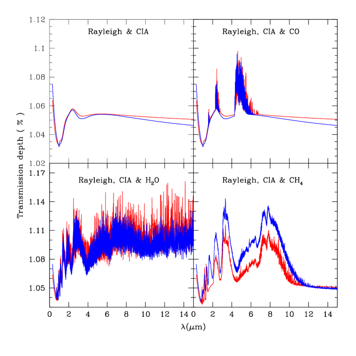
Figure 1: Comparison of transmission depth calculated by using two different models : (1) Exo-Transmit (red) and (2) Tau-REx (blue). A Jupiter-size planet with $T_{eq}=2700K$ and ${\rm g=30ms^{-2}}$ transiting a star with solar radius is considered in calculating the transmission depth.

In order to investigate the consistency and correctness in the chemistry involved, we derived the opacity due to a few individual molecules along with the opacity due to Rayleigh scattering and Collisional Induced Absorption (CIA) by using another model, Tau-REx (Waldmann, Tinetti, Rocchetto, et al., 2015). Tau-REx is an open source model which adopts line-lists from ExoMol (Tennyson & Yurchenko, 2012; Tennyson, Yurchenko, Al-Refaie, et al., 2016). By using the optical depth derived from the two different models, we calculate and compare the transmission depth for a jupiter size exoplanet with $T_{eq}=2700K$ and surface gravity ${\rm g=30ms^{-2}}$ transiting a solar type star. We set the abundances of the individual molecules CO, ${\rm H_{2}O}$ and ${\rm CH_{4}}$ at $10^{-4}$ and used the Beer-Bouguer-Lambert law and not the radiative transfer equations for calculating the transmission depth. Figure 1 shows that except for ${\rm CH_{4}}$, the results obtained by using the opacity derived from the two models are in good agreement. We will address this difference in a future paper as we limit the scope of the present work to the effect of scattering in the optical.

Using Exo-Transmit package we calculated the total extinction co-efficients (true absorption plus scattering) as well as the scattering co-efficients for a given $T-P$ profile and surface gravity. The albedo for single scattering at each wavelength and each pressure point is calculated by taking the ratio of the scattering co-efficient and the extinction co-efficient. We have incorporated all the species provided in the package and their EOS for solar metalicity without any change. The EOS for Rain-out condensation are adopted in all the calculations.

Finally, we have not included cloud opacity or additional scattering sources in our use of Exo-Transmit package. We have incorporated haze in our radiative transfer code and we discuss the cloud model in section 6. The Exo-Transmit software package is used only to calculate the atomic and molecular absorption and scattering coefficients.

4 Numerical method to solve the radiative transfer equations

We use the absorption and scattering co-efficients at different pressure level in the planetary atmosphere and calculate the line of sight optical depth as given in Equation 6. The wavelength dependent albedo for single scattering $\omega$ at different pressure levels is the ratio between the scattering co-efficients $\sigma(\lambda)$ and the extinction co-efficient $\chi(\lambda)$. We solve the multiple scattering radiative transfer equation as given in Equation 5 by using discrete space theory developed by Peraiah & Grant (1973). The numerical code is extensively used to solve the vector radiative transfer equations in order to calculate polarized spectra of cloudy brown dwarfs and self-luminous exoplanets (Sengupta & Marley, 2009, 2010; Marley & Sengupta, 2011; Sengupta & Marley, 2016; Sengupta, 2016, 2018). For the present work we use the scalar version of the same numerical code.

In this method we adopt the following steps :

1. The medium is divided into a number of “cells” whose thickness is defined by $\tau$. The thickness of each cell is less than a critical optical thickness $\tau_{c}$ which is determined on the basis of the physical characteristics of the medium .

2. The integration of the radiative transfer equation is performed on the cell which is bounded by a two dimensional grids $[\tau_{n},\tau_{n+1}]\times[\mu_{j-1/2},\mu_{j+1/2}]$.

3. These discrete equations are compared with the canonical equations of the interaction principle and the transmission and reflection operators of cells are obtained.

4. Lastly, all the cells are combined by “star” algorithm and the radiation field is obtained.

A detail description of the numerical method can be found in Peraiah & Grant (1973); Sengupta & Marley (2009).

Using 2.5 GHz Intel core i5 processor with 8 GB RAM, it takes typically 10-12 minutes for one complete run of the FORTRAN version of the code that calculates the transmission spectra for wavelength ranging from 0.3-30 $\mu{\rm m}$ with a total number of 4616 wavelength points. We have also developed python version of the code which provides the same results in shorter time.

In order to validate the numerical method as well as the molecular and atomic opacity used in the present work, we present in Figure 2 a comparison of our model spectrum with a model by Stephens et al. (2009) for a cloud-free methane-dwarf (T8) and with the observed Spex prism spectrum (Burgasser, McElwain, Kirkpatrick et al., 2004) of the T-dwarf 2MASSI J0415-0935. We also compare our model spectrum with the model presented by Fortney, Marley, Saumon et al. (2008) for a self-luminous directly imaged Jupiter-type exoplanets with $T_{eff}=600$K and surface gravity $g=30{\rm ms^{-2}}$. The comparison is presented in Figure 3. The model spectra and the temperature-pressure profiles for both the cases have kindly been provided by M. Marley (private communication).

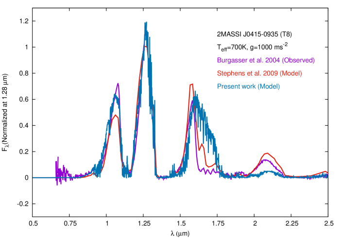
Figure 2: Comparison of model spectra with the observed Spex prism spectrum of a cloud-free brown dwarf (T8) 2MASSI J0415-0935.

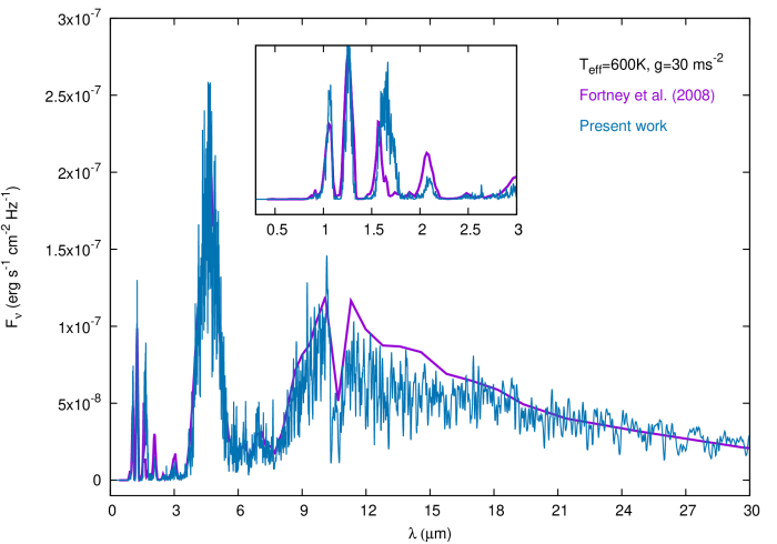
Figure 3: Comparison of model spectra for a self-luminous giant exoplanet

The slight miss-match of our synthetic spectrum with that of Stephens et al. (2009) at the infra-red region of the T-dwarf, as presented in Figure 2, is due to the disagreement in the opacity of methane as detected while comparing the model transmission depth derived by using Exo-Transmit and Tau-REx. The difference may also be attributed to a different elemental abundaces adopted. It is worth mentioning here that for the case of self-luminous exoplanet, the model spectrum of Fortney, Marley, Saumon et al. (2008) incorporates condensate cloud in the visible atmosphere while we have considered a cloud-free atmosphere.

5 The temperature-pressure profiles for irradiated exoplanets

The atmospheric temperature structure is an important input in the calculation of the transmission spectra. The self-consistent way to obtain the temperature-pressure ($T-P$) profile is to solve the radiative equilibrium equations simultaneously with the radiative transfer equations and hydrostatic equilibrium equations. The presence of molecules makes it more difficult to estimate the temperature structure as chemical equilibrium equations too need to be solved self-consistently. Further, for strongly irradiated exoplanets, the internal temperature is negligible compared to the temperature due to irradiation and the incident stellar flux at the top-most layer determines the atmospheric temperature structure as it interacts with the medium through absorption and scattering. Therefore, the atmospheric temperature at different depth is determined by the optical depth of the medium.. At the same time, the optical depth is governed by the temperature structure making it an involved and complicated numerical procedure. For stars, brown dwarfs and self-luminous exoplanets with weak or negligible irradiation, analytical formula for the $T-P$ profile in Grey or “slightly” non-Grey atmosphere was derived by Chandrasekhar (1960). Analytical formalisms of temperature structure for non-Grey strongly irradiated planets are presented by Hansen (2008); Guillot (2010); Parmentier & Guillot (2014); Parmentier, Guillot, Fortney et al. (2015). In order to model the transmission spectra of close-in exoplanets, isothermal $T-P$ profiles with $T(P)=T_{eq}$ were adopted by Sing, Fortney, Nikolov et al. (2016); Kempton, Lupu, Owusu-Asare et al. (2017); Goyal, Wakeford, Mayne et al. (2019). The radially inwards incident radiation usually penetrates quite deep, about 10-100bars pressure level. However, in the transit geometry considered for calculating the transmission spectrum, the atmosphere below approximately 1 bar pressure level is opaque because of the large path length that the radiation traverses. Therefore, a very small part of the overall atmosphere is probed in the transmission spectrum. So, isothermal approximation although not completely accurate, especially for hotter planets where temperature inversion due to the presence of TiO and VO becomes dominant, does not make much difference in the results for the comparatively cooler planets (Goyal, Mayne, Sing et al., 2018) with current observations.

In the present work, we have used the FORTRAN implementation of the analytical model for the $T-P$ profiles of non-Grey irradiated planets presented by Parmentier & Guillot (2014); Parmentier, Guillot, Fortney et al. (2015). This code available in public domain uses the functional form for Rosseland opacity provided by Valencia, Guillot, Parmentier et al (2013) which is based on the Rosseland opacities of Freedman, Marley & Lodder (2008). The analytical model takes into account the opacities both in the optical and in the infra-red region. The analytical models are compared with the state-of-the-art numerical models and the different coefficients in the analytical models are calibrated for a wide range of surface gravity and equilibrium temperature.

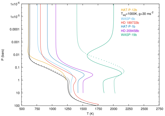
Figure 4: Temperature-Pressure ($T-P$) profiles of hot-Jupiters derived from the analytical formalisms presented by Parmentier, Guillot, Fortney et al. (2015). Dotted lines represent the corresponding $T-P$ profiles without the presence of TiO and VO in the atmosphere. $T_{eq}$ and $g$ used for each planet are listed in Table 1.

In Figure 4 we present the $T-P$ profiles derived by using the above mentioned computer code for a number of exoplanets with a wide range of surface gravity $g$ and equilibrium temperature $T_{eq}$. The values of $g$ and $T_{eq}$ for for various exoplanets are given in Table 1. We assumed that $T_{eq}$ for each exoplanets is the equilibrium temperature for zero albedo and the thermal profile is planet-averaged (see Parmentier & Guillot (2014)). Solar flux is assumed in the calculations. We have not considered a convective zone at the bottom of the models as such a zone should be situated much below the pressure level corresponding to $R_{P}$.

Table 1: Best fit parameters for the model transmission spectra in the infrared region of six exoplanets

Name	$T_{eq}$ (K)	g (${\rm ms^{-2}}$)	${\rm R_{P}(R_{J})}$	${\rm R_{*}(R_{\odot})}$	$n_{0}$	$d_{0}$ ($\mu$m )
WASP-19b	2050	14.2	1.34	1.01	0.0	0.0
HD 209458	1448	9.4	1.38	1.2	$5\times 10^{4}$	0.4
HAT-P-1b	1320	7.5	1.33	1.195	$3\times 10^{4}$	0.4
HD 189733	1200	21.4	1.19	0.8	$2\times 10^{5}$	0.4
HAT-P-12b	960	5.6	0.9	0.71	$1\times 10^{6}$	0.2
WASP-6b	1150	8.7	1.18	0.87	$2\times 10^{5}$	0.4

We have included the effect of TiO and VO on the $T-P$ profile. As shown in Figure 4, the effect is not significant for planets with $T_{eq}\leq 1000$K. However, as $T_{eq}$ increases, the atmospheric temperature increases significantly in the upper atmosphere due to the presence of TiO and VO in the atmosphere. For a planet as hot as WASP-19b ($T_{eq}$=2050K), the presence of TiO and VO introduces temperature inversion which disappears in the absence of TiO and VO. It’s worth mentioning here that in the absence of internal energy of the planet, the $T-P$ profile is used only to calculate the absorption and scattering co-efficients. The radiation field is determined by the incident stellar flux at the uppermost boundary.

6 Additional absorption and scattering due to atmospheric cloud/haze

Condensation cloud may play important role in shaping the transmission spectra of hot-Jupiters (Fortney, Shabram, Showman et al., 2010; Sing, Fortney, Nikolov et al., 2016). Under appropriate combination of temperature and surface gravity and based on chemical equilibrium process, cloud or haze may form in the visible region of the planetary atmosphere (Sudarsky, Burrows & Hubeny, 2003). It is well-known that the optical spectra of hotter L-brown dwarfs are shaped by the presence of condensation cloud (Cushing, Marley, Saumon et al., 2008) while in comparatively cooler T-brown dwarfs, cloud gets rain down below the visible atmosphere. Detail models of cloud and haze under chemical equilibrium in exo-planetary atmospheres have been presented by Ackerman & Marley (2001); Cooper, Sudarsky,Milsom, et al. (2003); Burrows, Budaj & Hubeny (2008).

In the present work we have considered a simple model for thin haze in the uppermost atmosphere following the approach of Griffith, Yelle, & Marley (1998); Saumon, Geballe, Leggett, et al. (2000). In this model the dust absorption and scattering cross-sections as well as the scattering phase function are calculated with the Mie theory of scattering (Bohren & Huffman, 1983). The cloud is confined within a thin region of the atmosphere bound by a base and deck. The vertical density distribution of the cloud particle is given by

$$n(P)=n_{0}\frac{P}{P_{0}},$$ (16)

where $n(P)$ is the number density of dust particle, $P$ is the ambient pressure, $P_{0}$ is the pressure at the base radius $R_{P}$ and $n_{0}$ is a free parameter with dimension of number density. The deck of the haze is fixed at 0.1 Pa pressure level and the base is located at 1.5-2.5 Pa. A log-normal size distribution of the dust particles given by

$$f(d)=\frac{d}{d_{0}}\times\exp\left[\frac{\ln(d/d_{0})}{\ln\sigma}\right]^{2}$$ (17)

where $d$ is the diameter of the dust particle, $d_{0}$ is the median diameter in the distribution and $\sigma$ is the standard deviation. Without loss of generality, in the present model, we fix $\sigma=1.3$ and the fraction of the maximum amplitude of the distribution function at which we set the cutoff of the distribution is taken to be 0.02. We have used the wavelength-dependent real and imaginary parts of the refractive index for amorphous Forsterite ${\rm(Mg_{2}SiO_{4})}$ which is believed to be the dominant constituent of atmospheric cloud.

It must be emphasized that although cloud or haze may play crucial role in determining the transmission as well as the emission spectra of hot-Jupiters, it is not necessary that the atmosphere of all hot-Jupiters should have cloud in the visible atmosphere. For low surface gravity and strong irradiation, cloud may evaporate from the atmosphere. On the other hand, for high surface gravity and low temperature, cloud may rain down below the visible region. The absence of alkaline absorption feature in the transmission spectra of many hot-Jupiters is usually interpreted as the presence of cloud. The whole purpose of this work is to invoke additional absorption and scattering opacities in the form of condensates and investigate how the optical spectra are affected by dust (Mie) scattering over Rayleigh scattering. In future, we shall incorporate more complicated and self-consistent cloud models.

7 Results and Discussions

We present the results for wavelength region ranging from near optical to infrared. Figure 5 shows the difference in the transmission depth calculated by solving the multiple scattering radiative transfer equations and by using Beer-Bouguer-Lambert law. The transmission depth presented by the model of Kempton, Lupu, Owusu-Asare et al. (2017) using Beer-Bouguer-Lambert law overlaps at all wavelengths with that of our model when $\omega=0$. Note that the opacity due to scattering is, however, included in the calculations of the optical depth.

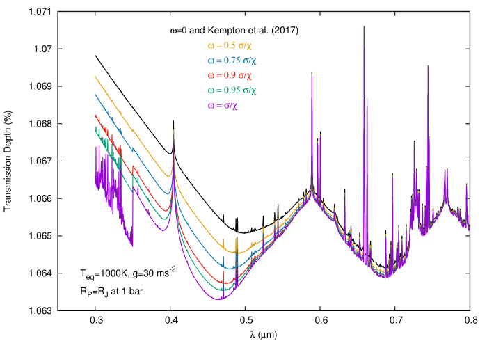
Figure 5: Transmission depth of a hot-Jupiter for different values of the scattering albedo $\omega=\sigma/\kappa$. The optical depth is unaltered for all cases. The model by Kempton, Lupu, Owusu-Asare et al. (2017) adopts Beer-Bouguer-Lambert law $I=I_{0}e^{-\tau}$ which overlaps with the present model when $\omega$ is set at zero. All of our models use the solution of the radiative transfer equations.

Considering a Jupiter-type exoplanet with $T_{eq}=1000$K and surface gravity $g=30{\rm ms^{-2}}$, we investigate the effect of scattering albedo by increasing its value while unaltering the optical depth due to scattering. Figure 5 shows that with the increase in the scattering albedo $\omega$, the amount of diffuse radiation due to scattering increases. Part of this diffuse radiation is added to the reduced stellar light that transmit the planetary atmosphere. Consequently the transmitted flux increases amounting in a decrease in the transmission depth. However, at wavelength longer than about 0.6 $\mu{\rm m}$, the Rayleigh scattering albedo becomes negligibly small and therefore the transmission spectra coincide to that without scattering. Hence, Figure 5 demonstrates that scattering plays an important role in determining the optical transmission spectra. Clearly, scattering contributes in two ways - (1) the opacity due to scattering adds up to the opacity due to pure absorption and hence increases the total optical depth which reduces the transmitted stellar flux and (2) increases the transmitted stellar flux by adding the diffuse radiation due to scattering to the outgoing stellar flux. The net effect yields into a decrease in the transmission depth as shown in Figure 5. However, at about $0.35{\rm\mu m}$, we notice a sudden rise in the transmission depth which remains unexplained. A possible reason could be a small but sharp increase in absorption by Na and K in the opacity data used which reduces the scattering albedo at that wavelength. The effect of scattering becomes negligible at wavelengths longer than about $0.7{\rm\mu m}$ where the opacity due to scattering also becomes negligible. This is also demonstrated in Figure 6. However, with the increase in the scattering co-efficients, the effect of scattering albedo is significant even in the near-infrared.

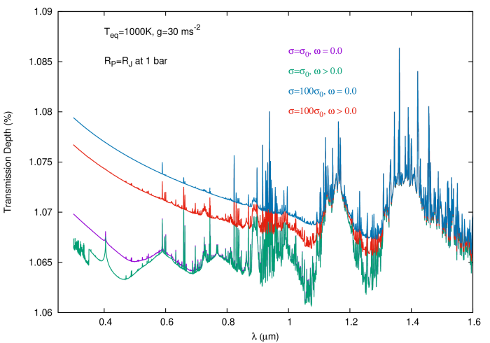
Figure 6: Comparison of transmission spectra with increased scattering opacity for zero and non-zero albedo. $\sigma_{0}$ is the actual opacity due to Rayleigh scattering derived by using solar system abundances. $\omega$ is the corresponding scattering albedo. The absorption co-efficients at all wavelengths are kept unaltered.

Figure 7 demonstrates that the transmission depth increases if the stellar flux passes through the deeper region of the atmosphere. If we consider that the planetary atmosphere through which the stellar flux is transmitted is extended up to a pressure level of 10 bar instead of 1 bar, the transmission depth increases by an amount given in Equation 3. Note that, in that case both the first and the second terms in the right hand side of Equation 3 should affect the transmission depth. However, Figure 7 shows a constant difference in the transmission depth even up to 10 $\mu{\rm m}$ implying that the change in the atmospheric radius $R_{PA}$ plays dominant role over the change in the transmitted flux. However, as mentioned in Section 5, because of the transit geometry considered for calculating the transmission spectrum, the atmosphere below approximately 1 bar pressure level is sufficiently opaque to the transmitted stellar radiation. Therefore, in all models we calculate $R_{PA}$ at 1 bar pressure level of the planetary atmosphere.

Similarly, Figure 8 shows that the transmission spectra does not differ significantly if isothermal temperature-pressure profile is considered instead of non-isothermal temperature-pressure profile derived through detail numerical procedure. However, as Figure 4 implies, the isothermal approximation is reasonable only if the planet is not strongly irradiated. For planets with equilibrium temperature higher than about 1400K, presence of TiO/VO introduces significant inversion in the temperature and therefore even at the upper layer of the atmosphere isothermal approximation may not be appropriate. Therefore, in order to calculate the transmission spectra in the optical region, accurate non-isothermal temperature-pressure profiles are needed to be used for relatively hotter planets.

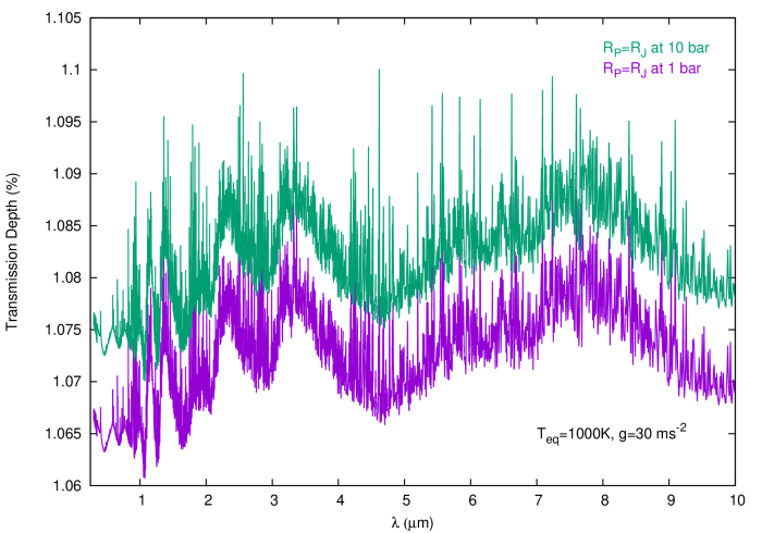
Figure 7: Comparison of transmission spectra with the base radius $R_{P}$ located at different pressure levels.

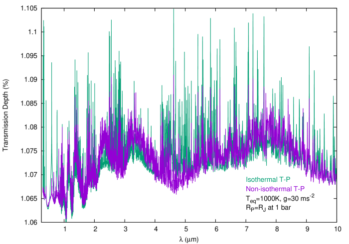
Figure 8: Comparison of transmission spectra with isothermal and non-isothermal temperature-pressure profile. For isorthermal case, the temperature is taken to be equal to $T_{eq}$ at all pressure points.

Using non-isothermal temperature-pressure profiles, we calculated the absorption and scattering coefficients and then the transmission depth is calculated by solving multiple scattering radiative transfer equations for plane-parallel stratification of the planetary atmosphere. We compare our model spectra for a few hot-Jupiters with the existing model spectra and observed data presented by Sing, Fortney, Nikolov et al. (2016). The model spectra of Sing, Fortney, Nikolov et al. (2016) and the observed data are available in public domain. The detail about these model grids and about the observed data are described in Sing, Fortney, Nikolov et al. (2016). The various physical parameters adopted in order to obtain best fit (by eye) at the infra-red region where scattering is negligible are listed in Table 1.

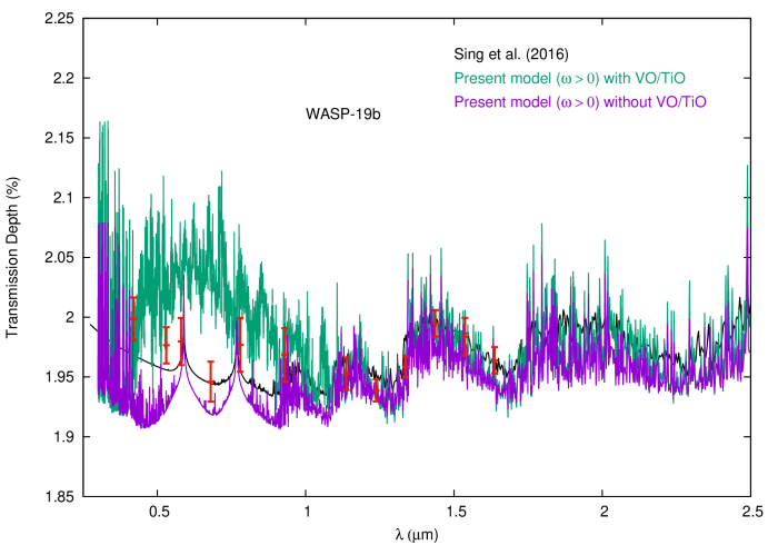
Figure 9: Comparison of model transmission spectra with and without the presence of VO and TiO and with the observed data (red) for WASP-19b.

In order to explain the high transmission depth in the optical, Sing, Fortney, Nikolov et al. (2016) incorporated additional Rayleigh scattering opacity by increasing the scattering cross section of hydrogen molecules 10 to 1000 times its value at 350 nm.. However, as can be seen in Figure 9, the present model for the exoplanet WASP-19b yields much higher transmission depth at optical region up to 1.0 $\mu{\rm m}$ than that presented by Sing, Fortney, Nikolov et al. (2016). We have not included any additional opacity source for this model. This difference is attributed to the presence of TiO and VO. In the absence of TiO and VO, the transmission depth profile qualitatively matches well with the model by Sing, Fortney, Nikolov et al. (2016). However, since diffusion by scattering reduces the transmission depth, the two models do not overlaps. The two models, however, match at wavelengths longer than 1.0 $\mu{\rm m}$ where the scattering is negligible..

As mentioned before, formation of cloud in the planetary atmosphere needs appropriate combination of temperature and surface gravity. Strong irradiation or strong thermal radiation can cause evaporation of the cloud while low temperature and high surface gravity may cause rain out of the condensates. The disappearance of atomic and molecular absorption lines in the optical is usually interpreted as the evidence of cloud or haze. However, for planetary atmosphere that has no or negligible thermal radiation, scattering by cloud may alter the absorption features in the transmission spectra. Presence of cloud or haze not only changes the total opacity of the atmosphere, it also alters the scattering albedo of the medium..

For all models except that of WASP-19b, we have included a thin haze in the upper atmosphere as described in section 6. In Figure 10, we present a comparison of the transmission spectra for HD 209458b with and without haze. We also present in the same figure the transmission spectra obtained with $\omega=0$. For both the cases - with zero and non-zero albedo, the total extinction i.e., the opacity due to true absorption as well as scattering is kept unchanged. With the inclusion of haze, the extinction increases yielding into higher optical depth at the upper atmosphere. The scattering albedo also changes due to cloud particles. Figure 10 shows that the transmission depth calculated with or without Rayleigh scattering albedo is much lower than that presented by Sing, Fortney, Nikolov et al. (2016). But a reasonably good match with the model by Sing, Fortney, Nikolov et al. (2016) in the optical is obtained by the inclusion of haze. The model spectra with and without haze converges at wavelength longer than 1.3 $\mu{\rm m}$. For this case, we have not presented the observed data as it fits with the model by Sing, Fortney, Nikolov et al. (2016) which fits the observed data in the optical.

Similarly, we have obtained reasonably good match with the model by Sing, Fortney, Nikolov et al. (2016) as well as with the observed data for HAT-P-1b by invoking haze in the planetary atmosphere. A comparison is presented in Figure 11. The transmission depth calculated without haze is significantly less than that calculated with haze. Note that in both the cases, the effect of scattering albedo is included. All the model spectra, however converges at wavelength longer than about 1.3 $\mu{\rm m}$ where scattering becomes negligible..

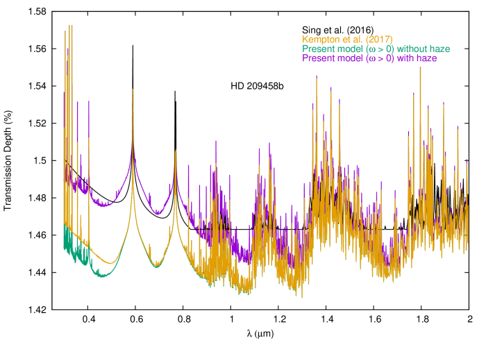
Figure 10: Comparison of model transmission spectra with and without the effect of Rayleigh scattering albedo and that by haze for exoplanet HD 209458b.

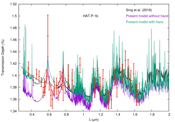
Figure 11: Comparison of model transmission spectra with and without the effect of haze and with the observed data (red) for HAT-P-1b.

The sharp increase in the values of observed transmission depth for HD 189733b and HAT-P-12b at wavelength shorter than 1.0 $\mu{\rm m}$ however do not fit our model transmission spectra even by increasing the scattering opacity a thousand times or by incorporating haze. Figure 12, however, demonstrates that inclusion of sub-micron size haze can produce comparable transmission spectrum that is obtained by invoking additional Rayleigh scattering opacity in the model by Kempton, Lupu, Owusu-Asare et al. (2017). Figure 13 also demonstrate the difference in the transmission spectra with and without the effect of scattering albedo when the scattering opacity is increased by a thousand times. Inclusion of haze results into transmission depth comparable to that presented by Sing, Fortney, Nikolov et al. (2016) in the optical only if the diffusion by scattering is excluded in the model. Clearly, the diffuse radiation due to scattering increases the transmitted flux resulting into a decrease in the transmission depth even up to 2.0 $\mu{\rm m}$. However, all the models converge at wavelengths longer than 2.0 $\mu{\rm m}$ as the scattering coefficient and hence the scattering albedo becomes negligible beyond this wavelength. We point out here that the rapid increase in the transmission depth at wavelength shorter than 0.5 micron may be due to other effects, e.g., stellar activities, star-spots etc.

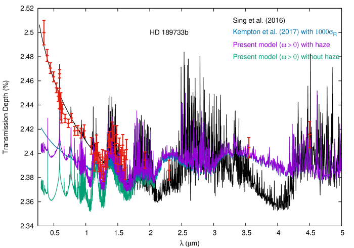
Figure 12: Comparison of observed data (red) and model transmission spectra for HD 189733b with and without haze in the upper atmosphere.

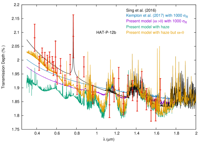
Figure 13: Comparison of observed data (red) and model transmission spectra for HATP-P-12b with and without haze in the upper atmosphere. The model transmission spectrum of Kempton, Lupu, Owusu-Asare et al. (2017) with thousand times of the actual scattering co-efficient is also presented for a comparison. Further, an atmospheric model with absorption by haze but without the effect of scattering albedo is presented in this figure.

Finally, we present in Figure 14 the model transmission spectra for WASP-6b with and without incorporating haze. It is worth mentioning that our numerical method ensures that the dust number density does not exceed the mass of heavy elements. Figure 14 shows that even with the maximum allowed values of dust number density, the transmission depth fails to fit the observed data in the optical region. We have achieved a good model fit with the observed data by increasing the Rayleigh scattering opacity eight times its original value in addition to incorporating haze. This indicates that a better cloud model is needed to fit the observed data.

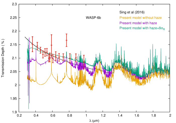
Figure 14: Comparison of observed data (red) and model transmission spectra for WASP-6b with and without haze.

8 Conclusions

We have presented detail numerical models of transmission spectra for hot jupiter-like exoplanets by solving the multiple scattering radiative transfer equations with non-zero scattering albedo instead of using the Beer-Bouguer-Lambert law. We have demonstrated that the solution of the radiative transfer equations that incorporate the diffuse reflection and transmission radiation field due to scattering yields significant changes in the transmission depth at the optical wavelength region, specially if the atmosphere is cloudy. However, at longer wavelength scattering becomes negligible and the transmission spectra overlap with that derived by using Beer-Bouguer-Lambert law. We compare our model spectra with the observed data and with two different theoretical models that include opacity due to scattering but do not take into account the diffuse reflection and transmission of the incident radiation field due to atmospheric scattering. We also include additional opacity and scattering albedo due to condensate cloud by adopting a simplified dust model. The most important message conveyed by the present work is that in order to analyze the observed optical transmission spectra of exoplanets, the retrieval models need to incorporate the scattering albedo that gives rise to diffused radiation field which is added to the stellar radiation transiting through the planetary atmosphere. Thus a correct and consistent procedure is to solve the multiple scattering radiative transfer equations. A substantial amount of diffuse stellar radiation increases the transmitted flux resulting into a decrease in the transmission depth. However, in the infrared wavelength region where the affect of scattering is negligible, Beer-Bouguer-Lambert law can very well be employed to calculate the transmission depth.

References

- Ackerman & Marley (2001) Ackerman, A. & Marley, M. S. 2001, ApJ, 556, 872.
- Asplund, Grevesse, Sauval & Scott (2009) Asplund M., Grevesse N., Sauval A. J., and Scott P., 2009, ARA&A, 47, 481.
- Barstow, Aigrain, Irwin et al., (2017) J. K. Barstow et al., 2017, ApJ, 834, 50.
- Bohren & Huffman (1983) Bohren, C. F., & Hu†man, D. R. 1983, Absorption and Scattering of Light by Small Particles (Wiley : New York).
- Brown (2001) Brown, T., ApJ, 553:1006-1026, 2001
- Burgasser, McElwain, Kirkpatrick et al. (2004) Burgasser, A. J., McElwain, M. W.., Kirkpatrick, J. D. et al. 2004, AJ , 127, 2856.
- Burrows, Budaj & Hubeny (2008) Burrows, A., Budaj, J. & Hubeny, I. 2008, ApJ, 678, 1436.
- Burrows et al. (2010) A. Burrows et al. 2010, ApJ, 719, 341.
- Burrows, (2014) Burrows, A. S., 2014, PNAS, 111 (35) 12601-12609
- Chandrasekhar (1960) Chandrasekhar, S. Radiative Transfer (New York: Dover, 1960).
- Cooper, Sudarsky,Milsom, et al. (2003) Cooper, C. S., Sudarsky, D., Milsom, J. A., Lunine, J. I. & Burrows, A. 2003, ApJ, 586, 1320.
- Cushing, Marley, Saumon et al. (2008) Cushing, M. C., Marley, M. S., Saumon, D. et al. 2008, ApJ, 678, 1372.
- de Kok & Stam (2012) de Kok, R. J. & Stam, D. M. 2012, Icarus, 221, 517.
- Fortney, Marley, Saumon et al. (2008) Fortney, J. J., Marley, M. S., Saumon, D. & Lodder, K. 2008, ApJ, 683, 1104.
- Fortney, Shabram, Showman et al. (2010) Fortney, J. J., Shabram, M., Showman, A. P., et al. 2010, ApJ, 709, 1396.
- Fortney (2018) Fortney, J. J. 2018, eprint arXiv:1804.08149.
- Freedman, Marley & Lodder (2008) Freedman, R. S., Marley, M. S., & Lodders, K. 2008, ApJS, 174, 504.
- Freedman, Lustig-Yaeger, Fortney et al. (2014) Freedman, R. S., Lustig-Yaeger, J., Fortney, J. J., et al., 2014, ApJS, 214, 25.
- Goyal, Mayne, Sing et al. (2018) Goyal J. M., Mayne, N. J., Sing, D. K., et al., 2018, MNRAS, 474, 5158.
- Goyal, Wakeford, Mayne et al. (2019) Goyal, J. M., Wakeford, H. R., Mayne, N. J. et al. 2019, MNRAS, 482, 4503.
- Gordon et al. (2017) I.E. Gordon, L.S. Rothman, C. Hill et al., 2017, J Quant Spectrosc Radiat Transfer 203, 3-69.
- Guillot (2010) Guillot, T. 2010, A&A, 520, A27.
- Griffith, Yelle, & Marley (1998) Griffith, C. A., Yelle, R. A., & Marley, M. S. 1998, Science, 282, 2063.
- Griffith (2014) Griffith, C. A., 201, 372, Philosophical Transactions of the Royal Society A: Mathematical, Physical and Engineering Sciences.
- Hansen (2008) Hansen, B. M. S. 2008, ApJS, 179, 484.
- Heng et al. (2018) K. Heng et al 2018, ApJS, 237, 29.
- Kempton, Lupu, Owusu-Asare et al. (2017) Kempton, E. M.-R., Lupu, R. E., Owusu-Asare, A., Slough, P., & Cale, B., 2016, PASP, 129, 1
- Lodders, K. (2003) Lodders, K. 2003, ApJ, 591, 1220.
- Lupu, Zahnle, Marley et al. (2014) Lupu, R. E., Zahnle, K., Marley, M. S., et al., 2014, ApJ, 784, 27
- Madhusudhan and Seager (2009) N. Madhusudhan and S. Seager, 2009, ApJ, 707, 24
- Marley & Sengupta (2011) Marley, M. S. & Sengupta, S. 2011, MNRAS,417, 2874.
- Parmentier & Guillot (2014) Parmentier, V. & Guillot, T. 2014, A&A, 562, A133.
- Parmentier, Guillot, Fortney et al. (2015) Parmentier, V., Guillot, T., Fortney, J. J., & Marley, M. S. 2015, A&A, 574, A35.
- Peraiah & Grant (1973) Peraiah, A., & Grant, I. P. 1973, J. Inst. Maths. Appl. 12, 75.
- Saumon, Geballe, Leggett, et al. (2000) Saumon, D., Geballe, T. R., Leggett, S. K., et al. (2000), ApJ, 541, 374.
- Seager & Sasselov (2000) Seager S., & Sasselov D. D., 2000, ApJ, 537, 916.
- Sengupta & Marley (2009) Sengupta, S. & Marley, M. S. 2009, ApJ, 707, 716.
- Sengupta & Marley (2010) Sengupta, S. & Marley, M. S. 2010, ApJL, 722, L142.
- Sengupta & Marley (2016) Sengupta, S. & Marley, M. S. 2016, ApJ, 824, 76..
- Sengupta (2016) Sengupta, S. 2016, AJ, 152, 98.
- Sengupta (2018) Sengupta, S. 2018, ApJ, 861, 41.
- Sing, Fortney, Nikolov et al. (2016) Sing, D. K., Fortney, J. J., Nikolov, N. et al. 2016, Nature, 529, 59.
- Sudarsky, Burrows & Hubeny (2003) Sudarsky, D., Burrows, A., & Hubeny, I. 2003, ApJ, 588, 1121.
- Stephens et al. (2009) Stephens, D. C. et al. 2009, ApJ, 702,154.
- Sudarsky, Burrows & Hubeny (2003) Sudarsky, D., Burrows, A., & Hubeny, I. 2003, ApJ, 588, 1121.
- Tennyson & Yurchenko (2012) Tennyson, J. & Yuschenko, S. N., 2012, MNRAS, 425, 21.
- Tennyson, Yurchenko, Al-Refaie, et al. (2016) Tennyson, J., Yurchenko, S. N., Al-Refaie, A. F., et al. 2016, J. Molecular Spectroscopy, 327, 73.
- Tinetti, Encrenaz & Coustenis (2013) Tinetti, G., Encrenaz, T. & Coustenis, A. 2013, AAR, 21, 63.
- Tinetti, Liang, et al. (2007) Tinetti, G., M. C. Liang et al., 2007, ApJ, 654, L99.
- Tsiaras, Waldmann, et al. (2018) A. Tsiaras, I. P. Waldmann et al 2018, AJ, 155 156.
- Valencia, Guillot, Parmentier et al (2013) Valencia, D., Guillot, T.,Parmentier, V. & Freedman, R. S. 2013, ApJ, 775, 10.
- Waldmann, Tinetti, Rocchetto, et al. (2015) Waldmann, I. P., Tinetti, G., Rocchetto, M. et al. 2015, ApJ, 802, 107.
- Yip et al. (2019) Yip K. H. et al., 2019, Integrating light-curve and atmospheric modelling of transiting exoplanets, arXiv:1811.04686.